A Combined Finite Element and Finite Volume
Method for Liquid Simulation

Abstract

We introduce a new Eulerian simulation framework for liquid animation that leverages both finite element and finite volume methods. In contrast to previous methods where the whole simulation domain is discretized either using the finite volume method or finite element method, our method spatially merges them together using two types of discretization being tightly coupled on its seams while enforcing second order accurate boundary conditions at free surfaces. We achieve our formulation via a variational form using new shape functions specifically designed for this purpose. By enabling a mixture of the two methods, we can take advantage of the best of two worlds. For example, finite volume method (FVM) result in sparse linear systems; however, complexity is encountered when unstructured grids such as tetrahedral or Voronoi elements are used. Finite element method (FEM), on the other hand, result in comparably denser linear systems, but the complexity remains the same even if unstructured elements are chosen; thereby facilitating spatial adaptivity. In this paper, we propose to use FVM for the majority parts to retain the sparsity of linear systems and FEM for parts where the grid elements are allowed to be freely deformed. An example of this application is locally moving grids. We show that by adapting the local grid movement to an underlying nearly rigid motion, numerical diffusion is noticeably reduced; leading to better preservation of structural details such as sharp edges, thin sheets and spindles of liquids.

1 Introduction

Spatial adaptivity has long been a promising tool for simulating large-scale physics phenomena, including water, smoke, and solids. In general, the key ingredients toward this goal live in the design of discretization of partial differential equations (PDE) on unstructured grids. In the past decades, a number of discretization techniques has been proposed such as finite volume method, finite element method, boundary element method and spectrum method.

They have both advantages and disadvantages. For example, spectrum method enables accurate temporal integration since the analytical solutions are known, but are often limited by the shape of simulation boundaries such as rectangles or spheres. Boundary element method reduces the degrees of freedom from volumetric $O(n^{3})$ to surface area $O(n^{2})$, but is only practical if a fast summation of spatially scattered Green’s functions is performed. Even though the summation could be accelerated via the fast multipole method (FMM), the linear system can not be pre-assembled, indicating that many efficacy-proven pre-conditioners are not accessible.

In fluids, finite volume method (FVM) have been historically the most favorable choice because FVM naturally encodes the concept of incompressibility as net zero of momentum flux over a control volume. Also, the resulting linear system becomes sparse (e.g., six entries per row for Laplacian on uniform grids). On the other hand, the complexity of FVM rapidly grows when the structure of grids deviates from the uniform cells. In particular, one is required to compute explicit Voronoi cells (or power particles) and its associated faces. In contrast, finite element method (FEM) gracefully handle such cases. This is possible because FEM encodes PDEs as volumetric integration over local support domains (a.k.a weak form); in doing this, exact volumetric integration of irregular shaped elements is computed by a quadrature rule. A quadrature rule requires only the knowledge of mapping from the spatial coordinates to the unit coordinate, which is straightforward for tetrahedral or hexahedral grids. At the cost of its versatility, FEM is often more expensive than FVM because nodes (essentially, the degrees of freedom) interact with diagonal grid elements. For example, a linearized Laplacian operator in FEM results in $27$ non-zeros per row on uniform grids.

In this paper, we aim to spatially select either FVM or FEM where desired. A major technical challenge in this end is how to design a strongly coupled discretization of two methods while minimizing artifacts. As an example of our application, we propose to populate locally moving grids to reduce numerical diffusion. Altogether, our contributions are summarized as follows.

• Strongly coupled FEM and FVM pressure solve: we propose a new method for calculating pressure using finite element method and finite volume method with second order accurate boundary conditions at free surfaces best satisfied.

• Spatial interpolation using MLS: we apply a MLS approximation to interpolate both velocity and level set where different discretization methods are spatially adjacent each other.

• Moving grids: we propose to move local grids along the velocity field, which we show lessens numerical diffusion arising from advection.

We verify the numerical accuracy of our combined finite element and finite volume method schemes through various tests. We also compare our simulation results with/without moving grids.

2 Previous Work

The history of research of computational fluid dynamics is long. In graphics, fluid animation stems back to Stam [1], which first incorporated the semi-Lagrangian advection scheme in graphics. Later, Fedkiw et al. [2] proposed a smoke simulation framework that introduces vorticity confinement. To this date, one standard grid-based liquid simulation method is based on combined Marker-And-Cell (MAC) grids and the level set method [3, 4]. Many researchers have extended these methods, such as imposing second order accurate Dirichlet boundary conditions [5, 6] by taking into account the distance from cell centers to the liquid surfaces. A broad overview of the history of these fluid simulations can be found in Bridson [7].

Octree grids are one of the most prevalent spatially adaptive methods. In computational mechanics, some work of this kind adopted an asymmetric discretization of Poisson’s equation for solving pressure [8]. Later, smoke and liquid simulations [9, 10], which can dynamically change the structure of octree were developed and become widespread because they can greatly reduce computational run time. The above methods were further improved to be able to handle pressure with second order accuracy on T-junctions [11]. Such methods can also be extended to enforce second order accuracy on solid [12, 13] and liquid surfaces [6] by means of the cut-cell or ghost fluid methods. However, since these methods are FVM-based, accurate discretization is not trivial near T-junction cells. Some researchers proposed a feasible fix to this issue, such as using power diagram [14] or modifying Poisson discretization [15].

Tetrahedral and hexahedral meshes for unstructured grids are one of the choices to produce adaptivity. Klingner et al. [16] were the first to use a spatially adaptive tetrahedral mesh for smoke simulation, and Chentanez et al. [17] extended to liquid simulation. While these methods suffer from the T-junction problem, Batty et al. [18] proposed a tetrahedral method that does not suffer from this problem, and Voronoi decomposition [19] is another example of a method that can handle boundaries. However, these discretizations are inherently complicated, especially the Poisson’equation for pressure solve, and there is still concern on the computational cost and memory consumption.

The use of moving grids has been proposed by English [20] and Fan [21]. The former is a method to prepare different grids for each moving grid and stitch them together by using Voronoi cells when constructing a linear system of pressure solve. The latter work was done for solid simulation but it was not shown for fluids. Aside from moving grids, hybrid grid-particle methods such as FLuid Implicit Particle (FLIP) [22] and Extended Narrow Band FLIP (EXNBFLIP) [23] are feasible alternatives to avoid numerical diffusion. They can be expected to improve the representation of details such as ballistic liquid motion. Combining them with moving grids is expected to provide stable calculations even with large time steps, and our method may be integrated with such methods.

3 Method

Our fluid solver is aimed to numerically solve the incompressible Euler equations

$$\frac{\partial\bm{u}}{\partial t}+\bm{u}\cdot\nabla\bm{u}=-\frac{1}{\rho}\nabla p+\bm{g},\hskip 8.5359pt\nabla\cdot\bm{u}=0,$$ (1)

where $\bm{u},t,\rho,p$ and $\bm{g}$ represent velocity, time, density, pressure, and gravity, respectively. In our discretization, we set $\rho=1$ for liquid and $\rho=0$ for the air. For the boundary conditions, we impose the Dirichlet boundary condition at the liquid-air boundary and the Neumann boundary condition at the liquid-solid boundary such that $\bm{n}\cdot\nabla p=0$ where $\bm{n}$ represents a solid normal. We use an adaptive time step method based on the CFL condition with the CFL number of around 2. For reasoning of such settings, we refer to Bridson’s book [7].

We outline our algorithm overview in Alg.1. In this section, we first discuss how to discretize the simulation domain by the combined FVM and FEM. Next, we detail how to construct a linear system for pressure solve as well as how to handle boundary conditions in section 3.2. Finally, we discuss how to handle advection with moving grids and how to interpolate quantities defined on grids.

Algorithm 1 Method Overview

1:Compute time step

2:Extrapolate velocity

3:Update position of moving grids

4:Advect levelset or density by $\bm{u}_{t}$

5:Advect velocity by $\bm{u}_{t}$

6:Reinitialize levelset

7:Pressure solve and project Velocity

8:Update velocity of moving grids

3.1 Discretization

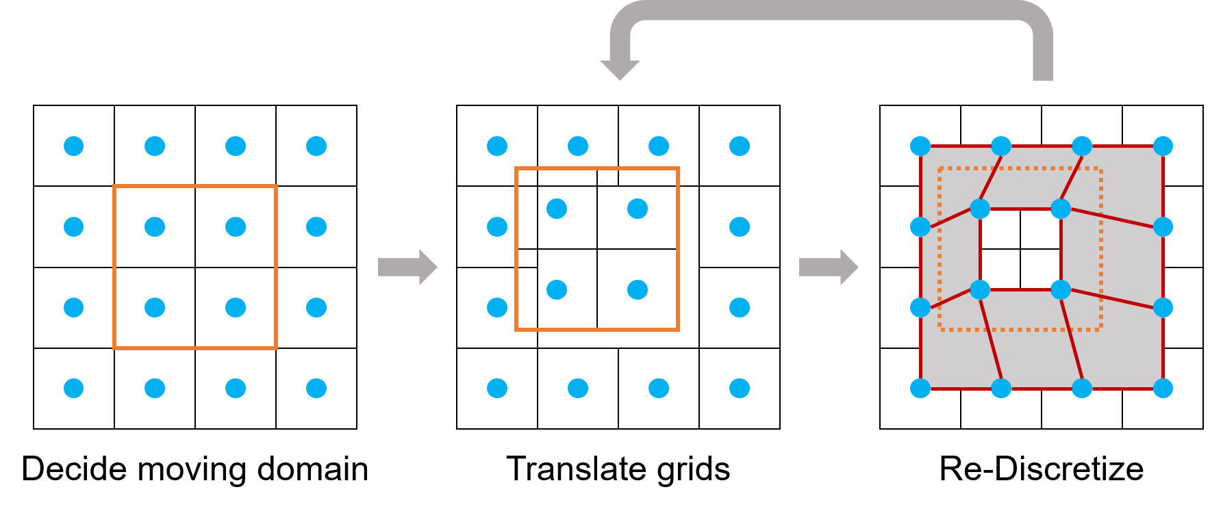
Figure 1: Discretization overview of moving grids. We specify the domain of the moving grids in advance (left). During the simulation, the position of the moving grids is updated according to the grid velocity $\bm{u}_{g}$ (middle). We use FEM (gray area) only at the edges of the moving grids (right).

In this paper, we use FVM for the majority part, and FEM is used only near the boundary with the moving grids. Figure 1 shows an overview of the discretization process. We construct the finite elements using cell-centered points as a node to simplify the pressure solve. When we set the moving grids, we assign information on which axis to move. The velocity of the moving grids $\bm{u}_{g}$ is set to be the largest velocity within the cells.

3.2 Pressure solve

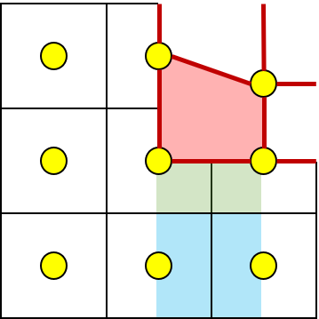
Figure 2: Volume integration and control volume adjustment. The control volume in FVM, colored as blue, is $\Delta x^{2}$. Red area is intergrated by Gaussian quadrature. The control volume is adjusted near the moving grids like the green area ($0.5\Delta x^{2}$).

The pressure in fluid simulation can be cast into solving the following kinetic energy minimization problem [12],

$$\underset{p}{\text{minimize}}\int_{\Omega}\frac{1}{2}\rho\left\|\bm{u^{*}}-\frac{\Delta t}{\rho}\nabla p\right\|^{2}dV,$$ (2)

where $\bm{u}^{*}$ denotes the velocity to be projected, and $\Omega$ represents the entire fluid domain. Since the pressure solve in our method is based on that of FVM and FEM, we will first give a brief explanation of both.

First, we describe the FVM, which accounts for the majority part in our method. To compute pressure, We solve a following linear system [15],

$$[\nabla]^{T}[V][A][F][\nabla]\{p\}=[\nabla]^{T}[V][A]\{\bm{u}^{*}\},$$ (3)

where $[\nabla]^{T},[\nabla],[V],[A],$ and $[F]$ respectively denotes a discrete divergence operator, a discrete gradient operator, a control volume of each face, a fluid area fraction and an inverse of liquid fraction of each face to achieve second order accuracy for Dirichlet boundary condition [6].

As for the pressure solve in FEM, we devise the method presented by Ibayashi et al [24]. We start by mapping the spatial coordinate $\bm{x}$ to unit coordinate $\bm{\xi}=[\xi,\eta,\zeta]$ similarly to various finite element methods. In this setting, the quantity $q$ at arbitrary coordinates in 3D can be rewritten as follows,

$$q(\bm{\xi})=\sum_{i=1}^{8}N_{i}(\bm{\xi})q_{i},$$ (4)

where $N_{i}$ is the trilinear shape function and is defined at the node of each element. Under this assumption, we construct a linear system as follows,

$$\sum^{n}_{e=1}\int_{\Omega_{e}}[\nabla_{e}]^{T}|J|[D][\nabla_{e}]\{p_{e}\}dV_{\xi}=\sum^{n}_{e=1}\int_{\Omega_{e}}[\nabla_{e}]^{T}|J|\bm{u}^{*}dV_{\xi},$$ (5)

where $\{p_{e}\}\in\mathbb{R}^{8\times 1}$ is the pressure stored on the nodes of $e$th element, and $J$ is the Jacobian matrix. $[\nabla_{e}]$ is the gradient operator given as,

$$[\nabla_{e}]_{ij}=[J^{-1}\nabla_{\xi}N(\bm{\xi})]_{i},\hskip 14.22636pt\nabla_{\xi}=\left(\frac{\partial}{\partial\xi},\frac{\partial}{\partial\eta},\frac{\partial}{\partial\zeta}\right)^{T}.$$ (6)

$[D]$ is defined as follows,

$$[D]=\frac{1}{\rho}M_{\phi},$$ (7)

where $M_{\phi}$ is the matrix that imposes a second order accuracy on the pressure solve proposed by Ibayashi et al [24]. We integrate Eq.(5) with an eight-point Gaussian quadrature integration scheme. We use the velocity of each element interpolated on Gaussian quadrature points for simplicity.

If we compare Eq.(3) and Eq.(5), we can see that volume factor $[V]$ and second order operator $[F]$ in the FVM correspond to $|J|$ and $[D]$ in the FEM, respectively. Since we have used the same spatial points of pressure definition in both methods, the pressure $p$ in each equation is considered to exactly coincide. As a result, we can properly compute the pressure by constructing a linear system that combines corresponding matrices. It is important to note that there is an overlap in the integration domain on the seams between FEM and FVM. We deal with this problem by adjusting the control volume of the FVM according to the occupancy of the finite elements as shown in the green area of Figure 2. Because the FEM uses Gaussian quadrature interpolation scheme and mapping it to the unit coordinate, it is difficult to adjust the integration range.

We project our second order operator such that the linear system becomes Symmetric Positive Definite (SPD) matrix that is numerically stable, as shown by previous work. The accuracy is therefore compromised, but we did not observe any visual artifact by this projection. A comparison with the fully second order solver is discussed in Section 5 on the subject of tilted pools.

Once the pressure is calculated, we have to project the velocity to the divergence-free field, so we subtract the pressure gradient

$$\{\bm{u}\}=\{\bm{u^{*}}\}-[F][\nabla]\{p\}.$$ (8)

For FEM, the velocity is defined at the center of the element, so the subtraction is averaged from the calculation points of the Gaussian quadrature interpolation scheme.

3.3 Interpolation

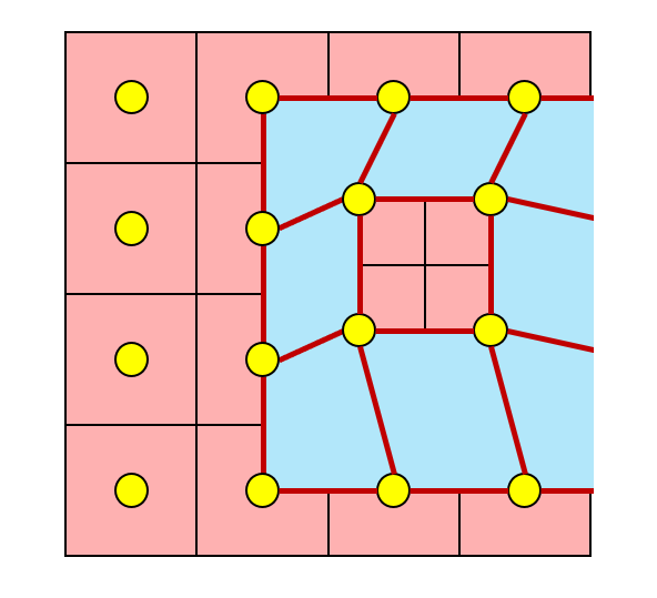
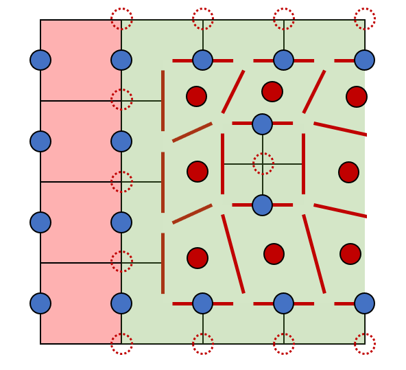
Figure 3: Our interpolation scheme for cell-centered value (left) and face-centered value (right). Yellow, dark blue, dark red, and the dark hollow red circle represent the location of cell-centered value, face-centered value of FVM, that of FEM, and the nodes where the element does not exist, respectively.

For the regularly distributed points use trilinear interpolation both for the FVM domain and the FEM domain to interpolate the values. For regions where two methods meet each other, we use different strategies depending on the location of quantity.

First, consider the cell-centered values. Because we share the location of the cell-centered values, we simply switch interpolation methods depending on whether the location where we want to interpolate in the FVM or the FEM region. For the FVM domain (red colored area of Figure 3), we interpolate the values by trilinear interpolation, and for the FEM domain (blue area), we use element-wise interpolation with the unit coordinate computed using Newton’s method.

Unlike the cell-centered values, the location of the face-centered values of FVM and FEM are not shared, therefore; we sort to Moving Least Square (MLS) interpolation method for face-centered values near the boundary (green area). As suggested by Ando et al. [15] we perform MLS interpolation based on the following equation,

$$q(\bm{p})=\begin{bmatrix}p_{x}&p_{y}&p_{z}&1\end{bmatrix}(Z^{T}DZ)^{-1}Z^{T}D\begin{bmatrix}\{q\}_{1}\\ \vdots\\ \{q\}_{n}\end{bmatrix},$$ (9)

$$Z=\begin{bmatrix}x_{1}&y_{1}&z_{1}&1\\ \vdots&\vdots&\vdots&\\ x_{n}&y_{n}&z_{n}&1\\ \end{bmatrix},\hskip 8.5359ptD=\rm{diag}\begin{pmatrix}\begin{bmatrix}N(\bm{p}-\bm{x}_{1},\Delta x)\\ \vdots\\ N(\bm{p}-\bm{x}_{n},\Delta x)\end{bmatrix}\end{pmatrix},$$ (10)

where $\bm{p}=[p_{x},p_{y},p_{z}],\bm{x}_{i}=[x_{i},y_{i},z_{i}],n,$ and $q$ denotes the query point, the position of the $i$th sample point, the number of sample points, and variable at the discrete point, respectively. We utilize such an interpolation scheme by using different ways of determining weight $N$ for each FVM and FEM values. For the FVM weights, we use

$$N_{FVM}(\bm{r},h)=\prod^{3}_{j=1}\rm{max}(1-\frac{||r_{j}||}{h},\epsilon),$$ (11)

where $\epsilon$ is the safety constant value. This weight is consistent with a simple tri-linear interpolation weight. For FEM, we first compute the unit coordinate $\bm{\xi}$ and use coefficients of the elemental interpolation as the FEM weights. To compute $\bm{\xi}$, we consider virtual elements composed by connecting the defining point of the velocity, that is the center of each element. As shown in the Figure 3, in the part where no element is defined, we assume that the element center is at the grid node point, and $\bm{\xi}$ is computed from this virtual elements. If not enough samples are collected, MLS interpolation can be stabilized by collecting samples from the surrounding area with weights $\epsilon$.

3.4 Advection

We use semi-Lagrangian advection scheme [1] for both the velocity and the levelset advection. In our method, the defining points of the physical quantities are updated at each simulation step. For this reason, we need to pay attention to the location of the physical quantities used in the advection term. The equation for updating the values by semi-Lagrangian method is as follows

$$q^{*}(\bm{x},t)=q(\bm{x}-\bm{u}(\bm{x},t)\Delta t,t)$$ (12)

where $q^{*}$ denotes the intermediate quantity after the advection, and $q$ denotes the quantity that will be advected. In our method, we can consider that $q$ is the quantity defined on the grid before updated. Fortunately, we can consider Eq.(12) as advection using relative velocity, because it is consistent with the derivation based on the following advection equation,

$$q^{*}(\bm{x},t)=q(\bm{x}-\bm{u}_{g}\Delta t-(\bm{u}(\bm{x},t)-\bm{u}_{g})\Delta t,t),$$ (13)

where the second term of the argument of $q$ represents the moving grid displacement, and the third term represents the advection by relative velocity. Such a strategy can be considered as the simple version of the advection method proposed in Chimera Grids [20]. The difference between our method and theirs is that we do not need to prepare several layers of ghost cells due to the continuity of our interpolation method as described in Section 3.3.

4 Results

We ran some experiments on a Linux machine with AMD Ryzen 9 5950X. We use Eigen library [25] to solve the linear system, and set the tolerant relative residual to $10^{-4}$ for pressure solve. We use the PDE-based approach [26] for the level set reinitialization process. We apply the marching cubes [27] for liquid surface extraction, and visualize them by Mitsuba [28]. In this section, we will evaluate the accuracy of the combined finite element and finite volume methods, and we show the benefits of simulation using moving grids.

4.1 Accuracy evaluation

Resolution	Cell centered	Face centered
$16^{2}$	$5.332\text{e-3}(\text{N / A})$	$4.349\text{e-3}(\text{N / A})$
$32^{2}$	$1.333\text{e-3}(2.00)$	$1.086\text{e-3}(2.00)$
$64^{2}$	$3.324\text{e-4}(2.00)$	$2.716\text{e-4}(2.00)$
$128^{2}$	$8.325\text{e-5}(2.00)$	$6.726\text{e-4}(2.01)$
$256^{2}$	$2.047\text{e-5}(2.02)$	$1.669\text{e-5}(2.01)$

Table 1: $L_{\infty}$ error and accuracy order of our interpolation scheme on quadratic field.

We evaluate our interpolation method with linear or quadratic fields, and the results are shown in Figure 4 and Figure 5. We set up a displaced grid and used the FEM around it as well as the discretization of the moving grids. We set the range as a $1\times 1$ dimensionless field, and each field is represented by the following equation.

Linear $$:f(x,y)=0.5(x+y)$$ (14)

Quadratic $$:f(x,y)=2\left\{(x-0.5)^{2}+(y-0.5)^{2}\right\}.$$ (15)

We convert the errors into the following log scale,

$$f(x,y)=1.0+0.1\log_{10}|\text{error}(x,y)|,$$ (16)

and visualized it in a heat map. Our interpolation method is able to reproduce the linear field with minimal errors. Because it is based on trilinear interpolation, there are some errors in the quadratic field, but it decreases at the second order as the resolution doubles. (Table 1).

We also tested the accuracy of our pressure solve on the horizontal and tilted pool examination. As illustrated in Figure 2, our pressure solve with first order accuracy could not project velocity to a divergence-free field, however, we can acquire divergence-free velocity using our second order pressure solve.

4.2 Simulation results using moving grids

	Fig.7		Half Reso of Fig.7
	Previous	Ours	Previous	Ours
Advection	92.01	102.05	4.27	6.20
Projection	1080.55	1097.69	35.48	37.21
Update moving grids	N/A	32.32	N/A	1.69
Total	1188.76	1249.69	40.67	46.07

Table 2: Timings (in second) per frame of previous and our method in the scene of Figure 7 and that with half resolution.

We ran some experiments using our method and compared them with the previous method [5]. Table 2 shows the computational time in the scene of Figure 7.

Figure 7 shows the results of the liquid objects falling experiment. In this test, we set moving grids with the same speed of the falling objects. This prevents missing details in the objects. From this result, we can see that our method with moving grids is able to suppress the effect of numerical diffusion. The computational time of our method is $1.05$ times longer than the standard liquid solve without our technique, and in particular, the advection part takes $1.11$ times longer. When it comes to the half resolution results, our method took $1.13$ times longer for the computational time, and $1.45$ times longer for the advection time. We discuss this point in Section 5.

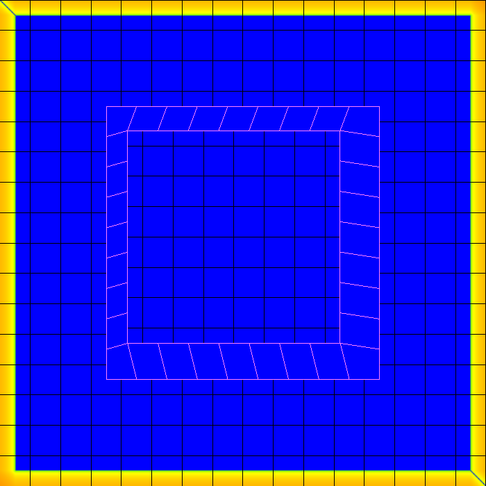
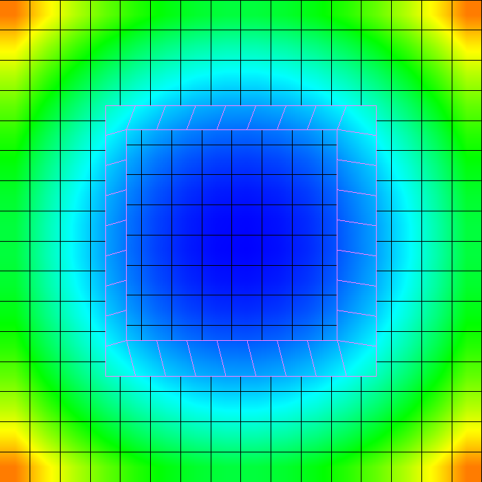
Figure 4: Interpolation results of cell centered values for linear (top) and quadratic (bottom) fields. Left: reproduced field. Right: error visualization.

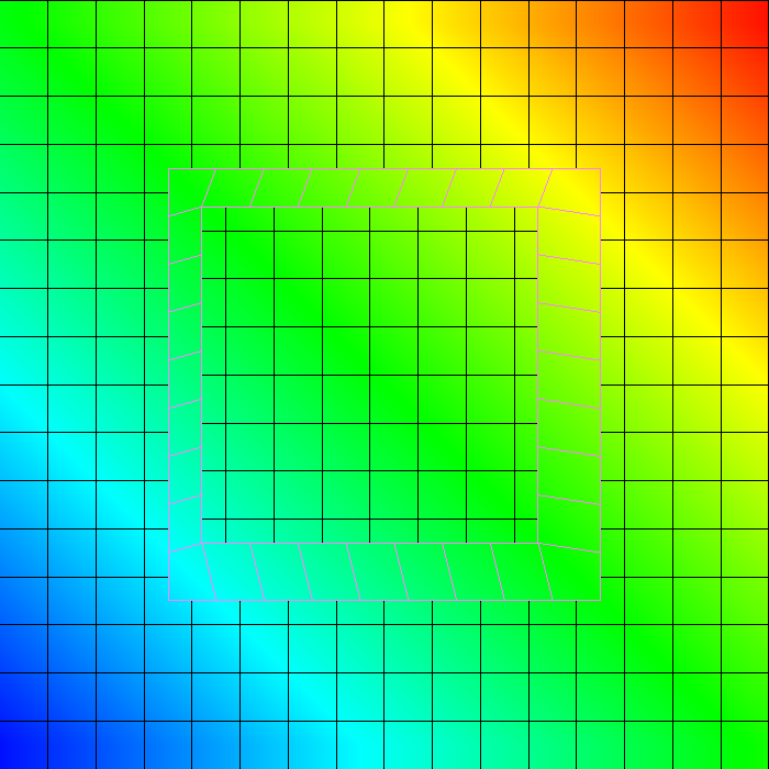
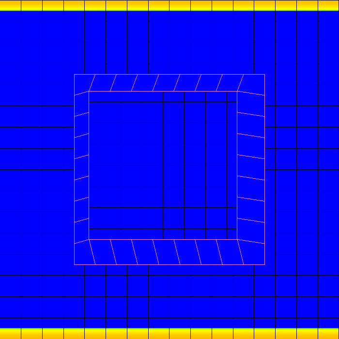
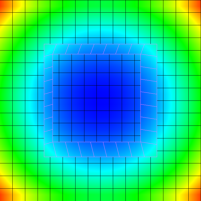
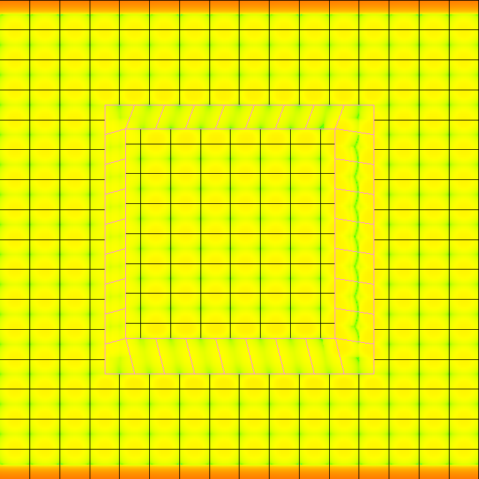
Figure 5: Interpolation results of face centered values for linear (top) and quadratic (bottom) fields. Left: reproduced field. Right: error visualization.

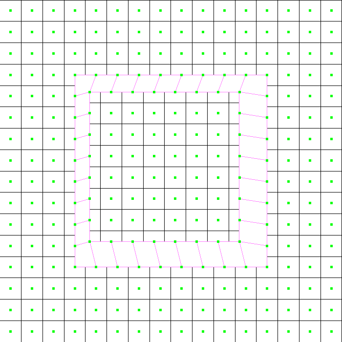
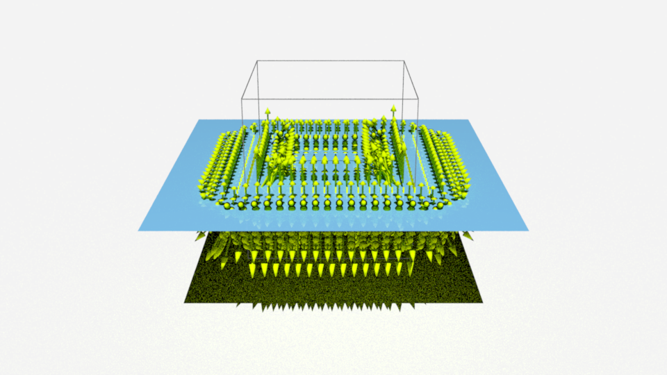
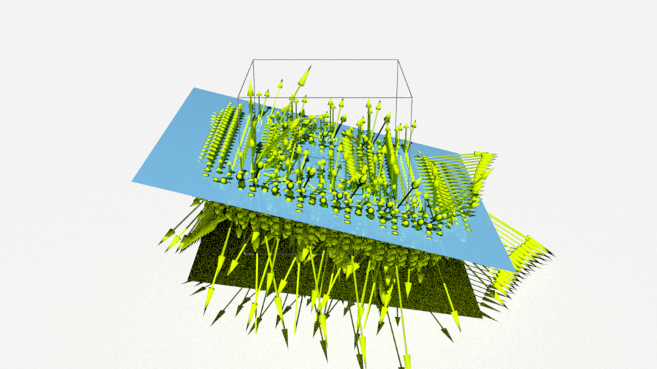
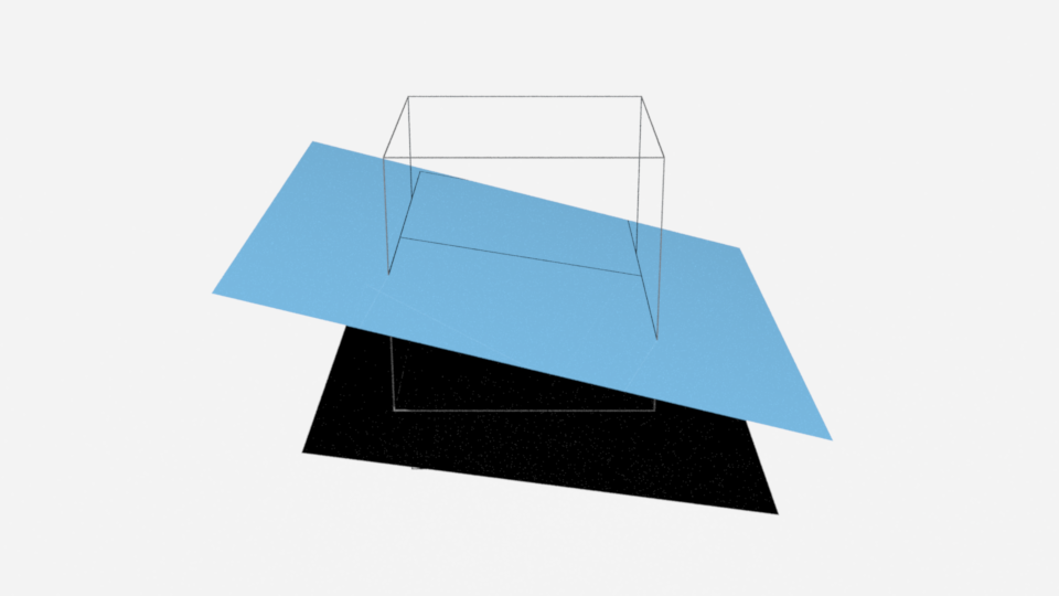
Figure 6: Results of our pressure solver test on the horizontal pool and tilted pool. Top one illustrates the simple visualization of grid geometry in 2D. We add strong gravity force in the direction normal to the liquid surface. Yellow arrows represents velocity after projection. Left: naive first order projection. Right: second order projection(SPD).

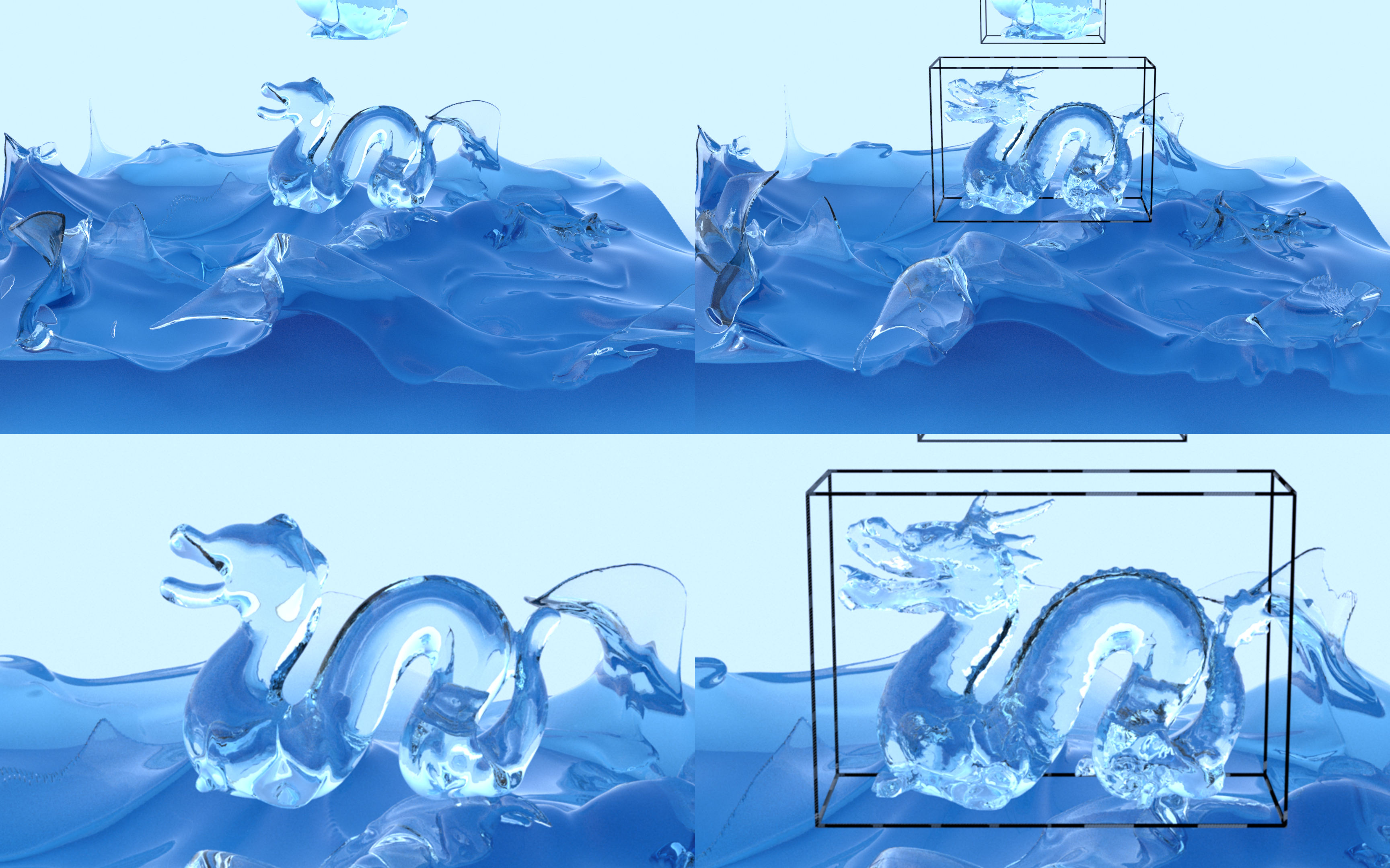
Figure 7: Comparison of previous and proposed methods on liquid objects falling into a pool simulated with grids of $600^{3}$ resolutions. Left: previous method. Right: our method.

5 Discussion and Conclusion

This paper presented a new Eulerian simulation framework for liquid simulation that leverages both finite element and finite volume methods, and we showed the numerical robustness of our MLS-based interpolation scheme and our new pressure solve. In addition, we showed the applicability of our method with moving grids, and showed that it is possible to suppress numerical diffusion.

As shown in the interpolation test of the quadratic field in Figure 4 and 5, even with trilinear interpolation, the error becomes worse as evaluation points get farther from the defining points. This indicates that covering the grid with moving grids of the same velocity as the liquid achieves that interpolation takes place near the defining point, which results in reduced error.

As for the pressure solver, we found that our projected SPD resulted in some errors, as shown in Figure 8. However, as explained in previous work [15], using the SPD matrix is a satisfactory alternative because it is stable and fast to converge.

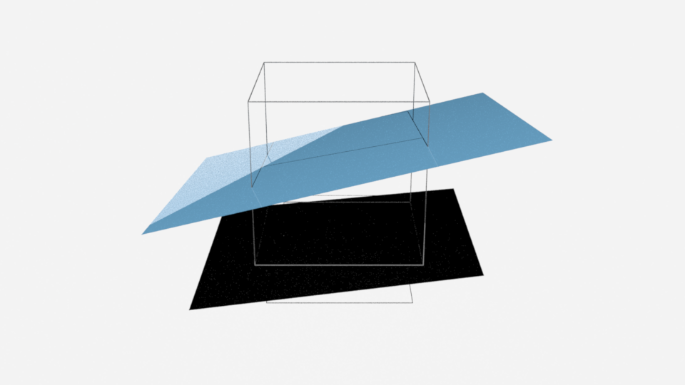
Figure 8: Comparison of SPD and second order accuracy. In the tilted pool, we observed some errors with SPD, but not for the case of imposing full second order accuracy.

Although our method is currently effective in suppressing numerical diffusion, it may also be effective with respect to reducing computational run time if the relative velocity can be used for optimization when computing time step under the CFL condition.

As for the performance, we are currently on the experimental stage, and as such, we did not optimize the code for faster performance. In particular, for advection, the search for MLS interpolation sample points has not been optimized, which results in many unnecessary calculations. However, since our method restricts the use of FEM to moving grid boundaries, the computational overhead is relatively small as the FEM portion decreases with increasing resolution. Of course, optimization is important, but the low overhead of using FEM is one of the advantages of our method.

In our experiment, we employed hexahedral elements, however, we believe that tetrahedral elements can be used as well at the cost of compromised the accuracy of the linear interpolation.

In the future work, it will be more meaningful if the moving grids region can be adaptively determined and if rotational motion can be considered. We are also considering the possibility of using finite elements for dealing with the complexity arising from T-junction in octree grids [15].

References

- [1] Jos Stam. Stable fluids. In Proceedings of the 26th Annual Conference on Computer Graphics and Interactive Techniques, SIGGRAPH ’99, pages 121–128, New York, NY, USA, 1999. ACM Press/Addison-Wesley Publishing Co.
- [2] Ronald Fedkiw, Jos Stam, and Henrik Wann Jensen. Visual simulation of smoke. In Proceedings of the 28th Annual Conference on Computer Graphics and Interactive Techniques, SIGGRAPH ’01, page 15–22, New York, NY, USA, 2001. Association for Computing Machinery.
- [3] Francis H. Harlow and J. Eddie Welch. Numerical Calculation of Time-Dependent Viscous Incompressible Flow of Fluid with Free Surface. Physics of Fluids, 8(12):2182–2189, December 1965.
- [4] N. Foster and D. Metaxas. Controlling fluid animation. In Proceedings Computer Graphics International, pages 178–188, 1997.
- [5] Nick Foster and Ronald Fedkiw. Practical animation of liquids. SIGGRAPH ’01, page 23–30, New York, NY, USA, 2001. Association for Computing Machinery.
- [6] Doug Enright, Duc Nguyen, Frederic Gibou, and Ron Fedkiw. Using the particle level set method and a second order accurate pressure boundary condition for free surface flows. In In Proc. 4th ASME-JSME Joint Fluids Eng. Conf., number FEDSM2003–45144. ASME, pages 2003–45144, 2003.
- [7] Robert Bridson. Fluid Simulation for Computer Graphics. A K Peters/CRC Press, September 2008.
- [8] Stéphane Popinet. Gerris: A tree-based adaptive solver for the incompressible euler equations in complex geometries. Journal of Computational Physics, 190:572–600, 10 2002.
- [9] Lin Shi and Yizhou Yu. Visual smoke simulation with adaptive octree refinement. 08 2004.
- [10] Frank Losasso, Frédéric Gibou, and Ron Fedkiw. Simulating water and smoke with an octree data structure. ACM Trans. Graph., 23(3):457–462, August 2004.
- [11] Frank Losasso, Ronald Fedkiw, and Stanley Osher. Spatially adaptive techniques for level set methods and incompressible flow. Computers & Fluids, 35(10):995–1010, 2006.
- [12] Christopher Batty, Florence Bertails, and Robert Bridson. A fast variational framework for accurate solid-fluid coupling. ACM Trans. Graph., 26(3):100, 2007.
- [13] Yen Ting Ng, Chohong Min, and Frédéric Gibou. An efficient fluid-solid coupling algorithm for single-phase flows. Journal of Computational Physics, 228(23):8807–8829, December 2009.
- [14] Mridul Aanjaneya, Ming Gao, Haixiang Liu, Christopher Batty, and Eftychios Sifakis. Power diagrams and sparse paged grids for high resolution adaptive liquids. ACM Trans. Graph., 36(4), July 2017.
- [15] Ryoichi Ando and Christopher Batty. A practical octree liquid simulator with adaptive surface resolution. ACM Trans. Graph., 39(4), July 2020.
- [16] Bryan M. Klingner, Bryan E. Feldman, Nuttapong Chentanez, and James F. O’Brien. Fluid animation with dynamic meshes. In ACM SIGGRAPH 2006 Papers, SIGGRAPH ’06, page 820–825, New York, NY, USA, 2006. Association for Computing Machinery.
- [17] Nuttapong Chentanez, Bryan E. Feldman, François Labelle, James F. O’Brien, and Jonathan R. Shewchuk. Liquid simulation on lattice-based tetrahedral meshes. In Proceedings of the 2007 ACM SIGGRAPH/Eurographics Symposium on Computer Animation, SCA ’07, page 219–228, Goslar, DEU, 2007. Eurographics Association.
- [18] Christopher Batty, Stefan Xenos, and Ben Houston. Tetrahedral embedded boundary methods for accurate and flexible adaptive fluids. In Proceedings of Eurographics, 2010.
- [19] Tyson Brochu, Christopher Batty, and Robert Bridson. Matching fluid simulation elements to surface geometry and topology. ACM Trans. Graph., 29(4), July 2010.
- [20] R. Elliot English, Linhai Qiu, Yue Yu, and Ronald Fedkiw. Chimera grids for water simulation. In Proceedings of the 12th ACM SIGGRAPH/Eurographics Symposium on Computer Animation, SCA ’13, page 85–94, New York, NY, USA, 2013. Association for Computing Machinery.
- [21] Ye Fan, Joshua Litven, David I. W. Levin, and Dinesh K. Pai. Eulerian-on-lagrangian simulation. 32(3), July 2013.
- [22] Yongning Zhu and Robert Bridson. Animating sand as a fluid. ACM Trans. Graph., 24(3):965–972, July 2005.
- [23] Takahiro Sato, Chris Wojtan, Nils Thuerey, Takeo Igarashi, and Ryoichi Ando. Extended Narrow Band FLIP for Liquid Simulations. Computer Graphics Forum, 2018.
- [24] H. Ibayashi, C. Wojtan, N. Thuerey, T. Igarashi, and R. Ando. Simulating liquids on dynamically warping grids. IEEE Transactions on Visualization and Computer Graphics, pages 1–1, 2018.
- [25] Gaël Guennebaud, Benoît Jacob, et al. Eigen v3. http://eigen.tuxfamily.org, 2010.
- [26] Giovanni Russo and Peter Smereka. A remark on computing distance functions. Journal of Computational Physics, 163:51–67, 2000.
- [27] William E. Lorensen and Harvey E. Cline. Marching cubes: A high resolution 3d surface construction algorithm. SIGGRAPH Comput. Graph., 21(4):163–169, August 1987.
- [28] Wenzel Jakob. Mitsuba renderer, 2010. http://www.mitsuba-renderer.org.