Stability and guaranteed error control of approximations to the Monge–Ampère equation

Abstract.

This paper analyzes a regularization scheme of the Monge–Ampère equation by uniformly elliptic Hamilton–Jacobi–Bellman equations. The main tools are stability estimates in the $L^{\infty}$ norm from the theory of viscosity solutions which are independent of the regularization parameter $\varepsilon$. They allow for the uniform convergence of the solution $u_{\varepsilon}$ to the regularized problem towards the Alexandrov solution $u$ to the Monge–Ampère equation for any nonnegative $L^{n}$ right-hand side and continuous Dirichlet data. The main application are guaranteed a posteriori error bounds in the $L^{\infty}$ norm for continuously differentiable finite element approximations of $u$ or $u_{\varepsilon}$.

1. Introduction

Overview

Let $\Omega\subset\mathbb{R}^{n}$, $n\geq 2$, be a bounded and convex domain. Given a nonnegative function $0\leq f\in L^{n}(\Omega)$ and continuous Dirichlet data $g\in C(\partial\Omega)$, the Monge–Ampère equation seeks the unique (convex) Alexandrov solution $u\in C(\overline{\Omega})$ to

(1.1) $$\det\mathrm{D}^{2}u=(f/n)^{n}\text{ in }\Omega\quad\text{and}\quad u=g\text{ on }\partial\Omega.$$

If the Dirichlet data $g\neq 0$ is non-homogenous, then we additionally assume that $\Omega$ is strictly convex. The re-scaling $\tilde{f}\coloneqq(f/n)^{n}$ of the right-hand side is not essential, but turns out convenient for purposes of notation. By the Alexandrov solution $u$ to (1.1) we mean a convex function $u\in C(\Omega)$ with $u=g$ on $\partial\Omega$ and

$$\mathcal{L}^{n}(\partial v(\omega))=\int_{\omega}\tilde{f}\,\mathrm{d}x\quad\text{for any Borel subset }\omega\subset\Omega.$$

The left-hand side denotes the Monge–Ampère measure of $\omega$, i.e., the $n$-dimensional Lebesgue measure of all vectors in the subdifferential $\partial v(\omega)\coloneqq\cup_{x\in\omega}\partial v(x)$ where $\partial v(x)$ is the usual subdifferential of $v$ in a point $x$. We remark that this solution concept admits more general right-hand sides, which are, however, not disregarded in this work. For further details, we refer to the monographs [13, 11]. It is known [1] that the Alexandrov solution to (1.1) exists and is unique. In addition, it was shown [4] that if $f\in C^{0,\alpha}(\Omega)$, $0<\lambda\leq f\leq\Lambda$, and $g\in C^{1,\beta}(\partial\Omega)$ with positive constants $0<\alpha,\beta<1$ and $0<\lambda\leq\Lambda$, then $u\in C(\overline{\Omega})\cap C^{2,\alpha}_{\text{loc}}(\Omega)$.

It is known [14, 10] that (1.1) can be equivalently formulated as a Hamilton–Jacobi–Bellman (HJB) equation, a property that turned out useful for the numerical solution of (1.1) [10, 12]; one of the reasons being that the latter is elliptic on the whole space of symmetric matrices $\mathbb{S}\subset\mathbb{R}^{n\times n}$ and, therefore, the convexity constraint is automatically enforced by the HJB formulation. For nonnegative continuous right-hand sides $0\leq f\in C(\Omega)$, the Monge–Ampère equation (1.1) is equivalent to

$$F_{0}(f;x,\mathrm{D}^{2}u)=0\text{ in }\Omega\quad\text{and}\quad u=g\text{ on }\partial\Omega$$

with $F_{0}(f;x,M)\coloneqq\sup_{A\in\mathbb{S}(0)}(-A:M+f\sqrt[n]{\det A})$ for any $x\in\Omega$ and $M\in\mathbb{R}^{n\times n}$. Here, $\mathbb{S}(0)\coloneqq\{A\in\mathbb{S}:A\geq 0\text{ and }\mathrm{tr}\,A=1\}$ denotes the set of positive semidefinite symmetric matrices $A$ with unit trace $\mathrm{tr}\,A=1$. Since $F_{0}$ is only degenerate elliptic, the regularization scheme proposed in [12] replaces $\mathbb{S}(0)$ by a compact subset $\mathbb{S}(\varepsilon)\coloneqq\{A\in\mathbb{S}(0):A\geq\varepsilon\}\subset\mathbb{S}(0)$ of matrices with eigenvalues bounded from below by the regularization parameter $0<\varepsilon\leq 1/n$. The solution $u_{\varepsilon}$ to the regularized PDE solves

(1.2) $$F_{\varepsilon}(f;x,\mathrm{D}^{2}u_{\varepsilon})=0\text{ in }\Omega\quad\text{and}\quad u_{\varepsilon}=g\text{ on }\partial\Omega$$

where, for any $x\in\Omega$ and $M\in\mathbb{R}^{n\times n}$, the function $F_{\varepsilon}$ is defined as

(1.3) $$F_{\varepsilon}(f;x,M)\coloneqq\sup\nolimits_{A\in\mathbb{S}(\varepsilon)}(-A:M+f\sqrt[n]{\det A}).$$

In two space dimensions $n=2$, uniformly elliptic HJB equations satisfy the Cordes condition [15] and this allows for a variational setting for (1.2) with a unique strong solution $u_{\varepsilon}\in H^{2}(\Omega)$ in the sense that $F_{\varepsilon}(f;x,\mathrm{D}^{2}u_{\varepsilon})=0$ holds a.e. in $\Omega$ [18, 19]. The paper [12] establishes uniform convergence of $u_{\varepsilon}$ towards the generalized solution $u$ to the Monge–Ampère equation (1.1) as $\varepsilon\searrow 0$ under the assumption $g\in H^{2}(\Omega)\cap C^{1,\alpha}(\overline{\Omega})$ and that $0\leq f\in L^{2}(\Omega)$ can be approximated from below by a pointwise monotone sequence of positive continuous functions.

Contributions of this paper

The variational setting of (1.2) in two space dimensions leads to $H^{2}$ stability estimates that deteriorate with $\varepsilon^{-1}\to\infty$ as the regularization parameter $\varepsilon\to 0$ vanishes. This can be explained by the regularity of Alexandrov solutions to the Monge–Ampère equation (1.1) as they are, in general, not in $H^{2}(\Omega)$ without additional assumptions on the domain $\Omega$ and the data $f,g$. Consequently, error estimates in the $H^{2}$ norm may not be of interest, and the focus is on error estimates in the $L^{\infty}$ norm.

The analysis departs from the following $L^{\infty}$ stability estimate that arises from the Alexandrov maximum principle. If $v_{1},v_{2}\in C(\overline{\Omega})$ are viscosity solutions to $F_{\varepsilon}(f_{j};x,\mathrm{D}^{2}v_{j})=0$ in $\Omega$ with $0\leq\varepsilon\leq 1/n$ and $f_{1},f_{2}\in C(\overline{\Omega})$, then

(1.4) $$\|v_{1}-v_{2}\|_{L^{\infty}(\Omega)}\leq\|v_{1}-v_{2}\|_{L^{\infty}(\partial\Omega)}+C(n,\mathrm{diam}(\Omega))\|f_{1}-f_{2}\|_{L^{n}(\Omega)}.$$

The constant $C(n,\mathrm{diam}(\Omega))$ exclusively depends on the dimension $n$ and the diameter $\mathrm{diam}(\Omega)$ of $\Omega$, but not on the ellipticity constant of (1.2) or on the regularization parameter $\varepsilon$. Consequently, this allows for control of the $L^{\infty}$ error even as $\varepsilon\to 0$. By density of $C(\overline{\Omega})$ in $L^{n}(\Omega)$, the $L^{\infty}$ stability estimate (1.4) can be extended to solutions $v_{1},v_{2}\in C(\overline{\Omega})$ for $0<\varepsilon\leq 1/n$ (or $\varepsilon=0$ if $f_{1},f_{2}\geq 0$) with the following two applications. First, this paper establishes, in extension to [12], uniform convergence of (generalized) viscosity solutions $u_{\varepsilon}$ of the regularized PDE (1.2) to the Alexandrov solution $u\in C(\overline{\Omega})$ of the Monge–Ampère equation (1.2) under the (essentially) minimal assumptions $0\leq f\in L^{n}(\Omega)$ and $g\in C(\partial\Omega)$ on the data. Second, (1.4) provides guaranteed error control in the $L^{\infty}$ norm (even for inexact solve) for $H^{2}$ conforming FEM.

Outline

The principal tool we use for establishing our results is the celebrated Alexandrov maximum principle. It provides an upper bound for the $L^{\infty}$ norm of any convex function in dependence of its Monge–Ampère measure.

Lemma 1.1 (Alexandrov maximum principle).

There exists a constant $c_{n}$ solely depending on the dimension $n$ such that any convex function $v\in C(\overline{\Omega})$ with homogenous boundary data $v|_{\partial\Omega}=0$ over an open bounded convex domain $\Omega$ satisfies

(1.5) $$|v(x)|^{n}\leq c_{n}^{n}\mathrm{dist}(x,\partial\Omega)\mathrm{diam}(\Omega)^{n-1}\mathcal{L}^{n}(\partial v(\Omega))\quad\text{for any }x\in\Omega.$$

Proof.

This is [11, Theorem 2.8] and the constant $c_{n}\coloneqq(2(2\pi)^{n/2-1}/((n-1)!!n)$ arises therein from the $n$-dimensional volume formula for a cone $\mathcal{C}\subset\partial v(\Omega)$. If $n=2$, then $c_{2}=1$. ∎

The remaining parts of this paper are organized as follows. Section 2 establishes $L^{\infty}$ stability estimates for viscosity solutions to the HJB equation (1.2) for all parameters $0\leq\varepsilon\leq 1/n$ in any space dimension. Section 3 provides a proof of convergence of the regularization scheme. A posteriori error estimates for the discretization error in the $L^{\infty}$ norm for $H^{2}$-conforming FEM are presented in Section 4. The three numerical experiments in Section 5 conclude this paper.

Standard notation for function spaces applies throughout this paper. Let $C^{k}(\Omega)$ for $k\in\mathbb{N}$ denote the space of scalar-valued $k$-times continuously differentiable functions. Given a positive parameter $0<\alpha\leq 1$, the Hölder space $C^{k,\alpha}(\Omega)$ is the subspace of $C^{k}(\overline{\Omega})$ such that all partial derivates of order $k$ are Hölder continuous with exponent $\alpha$. For any set $\omega\subset\mathbb{R}^{n}$, $\chi_{\omega}$ denotes the indicator function associated with $\omega$. For $A,B\in\mathbb{R}^{n\times n}$, the Euclidean scalar product $A:B\coloneqq\sum_{j,k=1}^{n}A_{jk}B_{jk}$ induces the Frobenius norm $|A|\coloneqq\sqrt{A:A}$ in $\mathbb{R}^{n\times n}$. The notation $|\cdot|$ also denotes the absolute value of a scalar or the length of a vector. The relation $A\leq B$ of symmetric matrices $A,B\in\mathbb{S}$ holds whenever $B-A$ is positive semidefinite.

2. Stability estimate

We first recall the concept of viscosity solutions to the HJB equation (1.2).

Definition 2.1 (viscosity solution).

Let $f\in C(\Omega)$ and $0\leq\varepsilon\leq 1/n$ be given. A function $v\in C(\overline{\Omega})$ is a viscosity subsolution (resp. supersolution) to $F_{\varepsilon}(f;x,\mathrm{D}^{2}v)=0$ if, for all $x_{0}\in\Omega$ and $\varphi\in C^{2}(\Omega)$ such that $v-\varphi$ has a local maximum (resp. minimum) at $x_{0}$, $F_{\varepsilon}(f;x,\mathrm{D}^{2}\varphi)\leq 0$ (resp. $F_{\varepsilon}(f;x,\mathrm{D}^{2}\varphi)\geq 0$). If $v$ is viscosity sub- and supersolution, then $v$ is called viscosity solution to $F_{\varepsilon}(f;x,\mathrm{D}^{2}v)=0$.

The following result provides the first tool in the analysis of this section.

Lemma 2.2 (classical comparison principle).

Given $0\leq\varepsilon\leq 1/n$ and a continuous right-hand side $f\in C(\Omega)$, where we assume $f\geq 0$ if $\varepsilon=0$, let $v^{*}\in C(\overline{\Omega})$ resp. $v_{*}\in C(\overline{\Omega})$ be a super- resp. subsolution to the PDE

(2.1) $$F_{\varepsilon}(f;x,\mathrm{D}^{2}v)=0\text{ in }\Omega.$$

If $v_{*}\leq v^{*}$ on $\partial\Omega$, then $v_{*}\leq v^{*}$ in $\overline{\Omega}$.

Proof.

The proof applies the arguments from [7, Section 3] to the PDE (2.1) and can follow [10, Lemma 3.6] with straightforward modifications; further details are therefore omitted. ∎

An extended version of Lemma 2.2 below is the following.

Lemma 2.3 (comparison principle).

Given any $0\leq\varepsilon_{*}\leq\varepsilon^{*}\leq 1/n$ and $f_{*},f^{*}\in C(\Omega)$ with $f_{*}\leq f^{*}$ in $\Omega$, where we assume $f_{*}\geq 0$ if $\varepsilon_{*}=0$, let $v_{*},v^{*}\in C(\overline{\Omega})$ be viscosity solutions to

$$F_{\varepsilon^{*}}(f_{*};x,\mathrm{D}^{2}v^{*})=0\text{ in }\Omega\quad\text{and}\quad F_{\varepsilon_{*}}(f^{*};x,\mathrm{D}^{2}v_{*})=0\text{ in }\Omega.$$

If $v_{*}\leq v^{*}$ on $\partial\Omega$, then $v_{*}\leq v^{*}$ in $\overline{\Omega}$.

Proof.

Given any test function $\varphi\in C^{2}(\Omega)$ and $x\in\Omega$ such that $v^{*}-\varphi$ has a local minimum at $x$, then $F_{\varepsilon^{*}}(f_{*};x,\mathrm{D}^{2}v^{*})=0$ in the sense of viscosity solutions implies $0\leq F_{\varepsilon^{*}}(f_{*};x,\mathrm{D}^{2}\varphi(x))$. This, $f_{*}\leq f^{*}$ in $\Omega$, and $\mathbb{S}(\varepsilon^{*})\subset\mathbb{S}(\varepsilon_{*})$ show

(2.2) $$0\leq F_{\varepsilon^{*}}(f_{*};x,\mathrm{D}^{2}\varphi(x))\leq F_{\varepsilon_{*}}(f^{*};x,\mathrm{D}^{2}\varphi(x)),$$

whence $v^{*}$ is viscosity supersolution to the PDE $F_{\varepsilon_{*}}(f^{*};x,\mathrm{D}^{2}v_{*})=0$. Therefore, the comparison principle from Lemma 2.2 with $v_{*}\leq v^{*}$ on $\partial\Omega$ concludes $v_{*}\leq v^{*}$ in $\overline{\Omega}$. ∎

The comparison principle from Lemma 2.2 allows for the existence and uniqueness of viscosity solutions (1.2) by Perron’s method.

Proposition 2.4 (properties of HJB equation).

Given any $0\leq\varepsilon\leq 1/n$, $f\in C(\Omega)\cap L^{n}(\Omega)$, where we assume $f\geq 0$ if $\varepsilon=0$, and $g\in C(\partial\Omega)$, there exists a unique viscosity solution $u\in C(\overline{\Omega})$ to the HJB equation (1.2). It satisfies (a)–(b):

1. (viscosity = Alexandrov) If $\varepsilon=0$ and $f\geq 0$ is nonnegative, then the viscosity solution to the HJB equation (1.2) and the Alexandrov solution to the Monge–Ampère equation (1.1) coincide.

2. (interior regularity for HJB) If $\varepsilon>0$ and $f\in C^{0,\alpha}(\Omega)$ with $0<\alpha<1$, then $u\in C(\overline{\Omega})\cap C^{2,\kappa}_{\text{loc}}(\Omega)$ with a constant $0<\kappa<1$ that solely depends on $\alpha$ and $\varepsilon$.

3. (interior regularity for Monge–Ampère) If $\varepsilon=0$, $f\in C^{0,\alpha}(\Omega)$ with $0<\alpha<1$, $f>0$ in $\overline{\Omega}$, and $g\in C^{1,\beta}(\partial\Omega)$ with $\beta>1-2/n$, then $u\in C(\overline{\Omega})\cap C^{2,\alpha}_{\text{loc}}(\Omega)$.

Proof.

On the one hand, an elementary reasoning as in the proof of Lemma 2.3 proves that the viscosity solution $v^{*}$ to the Poisson equation $F_{\varepsilon^{*}}(f_{*};x,\mathrm{D}^{2}v^{*})=0$ with $\varepsilon^{*}\coloneqq 1/n$, $f_{*}\coloneqq f$, and Dirichlet data $v^{*}=g$ on $\partial\Omega$ is a viscosity supersolution to (1.2). On the other hand, the Alexandrov solution $v_{*}$ to the Monge–Ampère equation (1.1) with the right-hand side $|f|$ [11, Theorem 2.14] is the viscosity solution to the HJB equation $F_{\varepsilon_{*}}(f^{*};x,\mathrm{D}^{2}v_{*})=0$ with $\varepsilon_{*}\coloneqq 0$, $f^{*}\coloneqq|f|$, and Dirichlet data $v_{*}=g$ on $\partial\Omega$ [13, Proposition 1.3.4]. Hence, the function $v_{*}$ is viscosity subsolution to (1.2). Therefore, Perron’s method [7, Theorem 4.1] and the comparison principle from Lemma 2.2 conclude the existence and uniqueness of viscosity solutions to (1.2). The combination of [10, Theorem 3.3 and Theorem 3.5] with [13, Proposition 1.3.4] implies the assertion in (a). The interior regularity in (b) is a classical result from [5, 17]. For the Monge–Ampère equation, the interior regularity in (c) holds under the assumption that the Alexandrov solution $u$ is strictly convex [11, Corollary 4.43]. Sufficient conditions for this are that $f>0$ is bounded away from zero and $g\in C^{1,\beta}(\partial\Omega)$ is sufficiently smooth [11, Corollary 4.11]. ∎

Some comments are in order, before we state a precise version of the $L^{\infty}$ stability estimate (1.4) from the introduction. In general, these estimates arise from the Alexandrov–Bakelman–Pucci maximum principle for the uniform elliptic Pucci operator, cf. [3] and the references therein for further details. However, the constant therein may depend on the ellipticity constant of $F_{\varepsilon}$ and therefore, on $\varepsilon$. In the case of the HJB equation (1.2) that approximates the Monge–Ampère equation (1.1) as $\varepsilon\to 0$, the Alexandrov maximum principle is the key argument to avoid a dependency on $\varepsilon$. Recall the constant $c_{n}$ from Lemma 1.1.

Theorem 2.5 ($L^{\infty}$ stability).

Given a nonnegative parameter $0\leq\varepsilon\leq 1/n$ and right-hand sides $f_{1},f_{2}\in C(\overline{\Omega})$, where we assume $f_{1},f_{2}\geq 0$ if $\varepsilon=0$, let $v_{1},v_{2}\in C(\overline{\Omega})$ be viscosity solutions to the HJB equation $F_{\varepsilon}(f_{j};x,\mathrm{D}^{2}v_{j})=0\text{ in }\Omega$ for $j\in\{1,2\}$. Then, for any subset $\omega\subset\Omega$,

(2.3) $$\|v_{1}-v_{2}\|_{L^{\infty}(\omega)}\leq\|v_{1}-v_{2}\|_{L^{\infty}(\partial\Omega)}+\frac{C}{n}\max_{x\in\overline{\omega}}\mathrm{dist}(x,\partial\Omega)^{1/n}\|f_{1}-f_{2}\|_{L^{n}(\Omega)}$$

with the constant $C\coloneqq c_{n}\mathrm{diam}(\Omega)^{(n-1)/n}$. In particular,

(2.4) $$\|v_{1}-v_{2}\|_{L^{\infty}(\Omega)}\leq\|v_{1}-v_{2}\|_{L^{\infty}(\partial\Omega)}+\frac{C}{n}(\mathrm{diam}(\Omega)/2)^{1/n}\|f_{1}-f_{2}\|_{L^{n}(\Omega)}.$$

Proof.

The proof is divided into two steps.

Step 1: The first step establishes (2.3) under the assumptions $f_{2}\leq f_{1}$ in $\overline{\Omega}$ and $v_{1}\leq v_{2}$ on $\partial\Omega$. For $f_{\Delta}\coloneqq f_{1}-f_{2}\geq 0$, let the sequence $(f_{\Delta,k})_{k\in\mathbb{N}}$ of smooth functions $f_{\Delta,k}\in C^{\infty}(\overline{\Omega})$ approximate $f_{\Delta}\in C(\overline{\Omega})$ from above such that $f_{\Delta}\leq f_{\Delta,k}$ and $0<f_{\Delta,k}$ in $\overline{\Omega}$ for all $k\in\mathbb{N}$ and $\lim_{k\to\infty}\|f_{k}-f_{\Delta,k}\|_{L^{\infty}(\Omega)}=0$. Let $w_{k}\in C(\overline{\Omega})$ be viscosity solutions to the PDE, for all $k\in\mathbb{N}$,

(2.5) $$F_{\varepsilon}(f_{\Delta,k};x,\mathrm{D}^{2}w_{k})=0\text{ in }\Omega\quad \text{and}\quad w_{k}=0\text{ on }\partial\Omega.$$

Since $v_{1}\leq v_{2}$ on $\partial\Omega$ and $f_{2}\leq f_{1}$ by assumption of Step 1, Lemma 2.3 proves

(2.6) $$v_{1}\leq v_{2}\text{ in }\overline{\Omega}.$$

Proposition 2.4(b)–(c) provides the interior regularity $w_{k}\in C^{2,\alpha}_{\mathrm{loc}}(\Omega)$ for some positive parameter $\alpha$ that (possibly) depends on $\varepsilon$. In particular, $w_{k}\in C^{2}(\Omega)$ is a classical solution to the PDE (2.5). We define the continuous function $v_{*}\coloneqq v_{2}-\|v_{1}-v_{2}\|_{L^{\infty}(\partial\Omega)}+w_{k}\in C(\overline{\Omega})$. Given any $x\in\Omega$ and $\varphi\in C^{2}(\Omega)$ such that $v_{*}-\varphi=v_{2}-(\|v_{1}-v_{2}\|_{L^{\infty}(\partial\Omega)}-w_{k}+\varphi)$ has a local maximum at $x$, the function $\psi\coloneqq\|v_{1}-v_{2}\|_{L^{\infty}(\partial\Omega)}-w_{k}+\varphi\in C^{2}(\Omega)$ is smooth and, therefore, an admissible test function in the definition of viscosity solutions. Since $v_{2}$ is viscosity solution to $F_{\varepsilon}(f_{2};x,\mathrm{D}^{2}v_{2})=0$, $F_{\varepsilon}(f_{2};x,\mathrm{D}^{2}\psi(x))\leq 0$ follows. This, $\mathrm{D}^{2}\psi=\mathrm{D}^{2}(\varphi-w_{k})$, the sub-additivity $\sup(X+Y)\leq\sup X+\sup Y$ of the supremum, $f_{\Delta}\leq f_{\Delta,k}$, and $F_{\varepsilon}(f_{\Delta,k};x,\mathrm{D}^{2}w_{k}(x))=0$ from (2.5) lead to

$$F_{\varepsilon}(f_{1};x,\mathrm{D}^{2}\varphi(x)) \leq F_{\varepsilon}(f_{2};x,\mathrm{D}^{2}\psi(x))+F_{\varepsilon}(f_{\Delta};x,\mathrm{D}^{2}w_{k}(x))$$

$$\leq F_{\varepsilon}(f_{2};x,\mathrm{D}^{2}\psi(x))+F_{\varepsilon}(f_{\Delta,k};x,\mathrm{D}^{2}w_{k}(x))\leq 0,$$

whence $v_{*}$ is viscosity subsolution to the PDE $F_{\varepsilon}(f_{1};x,\mathrm{D}^{2}v)=0$ in $\Omega$. Therefore, $v_{*}\leq v_{1}$ on $\partial\Omega$ by design and the comparison principle from Lemma 2.2 provide

(2.7) $$v_{*}\leq v_{1}\text{ in }\overline{\Omega}.$$

On the one hand, the zero function with $F_{\varepsilon}(f_{\Delta,k};x,0)\geq 0$ is a viscosity supersolution to $F_{\varepsilon}(f_{\Delta,k};x,\mathrm{D}^{2}w_{k})=0$. Hence, the comparison principle from Lemma 2.2 shows $w_{k}\leq 0$ in $\overline{\Omega}$. On the other hand, Proposition 2.4(a) proves that the Alexandrov solution $z_{k}\in C(\overline{\Omega})$ to $\det\mathrm{D}^{2}z_{k}=(f_{\Delta,k}/n)^{n}$ with homogenous boundary is viscosity solution to $F_{0}(f_{\Delta,k};x,\mathrm{D}^{2}z_{k})=0$ and Lemma 2.3 reveals $z_{k}\leq w_{k}$, whence $z_{k}\leq w_{k}\leq 0$ in $\overline{\Omega}$. Consequently, the Alexandrov maximum principle from Lemma 1.1 and $\mathcal{L}^{n}(\partial z_{k}(\Omega))^{1/n}=\|(f_{\Delta,k}/n)^{n}\|_{L^{1}(\Omega)}^{1/n}=\|f_{\Delta,k}\|_{L^{n}(\Omega)}/n$ imply

(2.8) $$0\leq-w_{k}\leq-z_{k}\leq\frac{C}{n}\max_{x\in\overline{\omega}}\mathrm{dist}(x,\partial\Omega)^{1/n}\|f_{\Delta,k}\|_{L^{n}(\Omega)}\quad\text{in }\overline{\omega}$$

for any subset $\omega\subset\Omega$. The combination of (2.6)–(2.8) with $v_{*}=v_{2}-\|v_{1}-v_{2}\|_{L^{\infty}(\partial\Omega)}+w_{k}$ results in

$$\|v_{1}-v_{2}\|_{L^{\infty}(\omega)}\leq\|v_{2}-v_{*}\|_{L^{\infty}(\omega)}=\|v_{1}-v_{2}\|_{L^{\infty}(\partial\Omega)}+\|w_{k}\|_{L^{\infty}(\omega)}$$

$$\leq\|v_{1}-v_{2}\|_{L^{\infty}(\partial\Omega)}+\frac{C}{n}\max_{x\in\overline{\omega}}\mathrm{dist}(x,\partial\Omega)^{1/n}\|f_{\Delta,k}\|_{L^{n}(\Omega)}$$ .

A passage of the right-hand side to the limit as $k\to\infty$ and $\lim_{k\to\infty}\|f_{\Delta,k}\|_{L^{n}(\Omega)}=\|f_{\Delta}\|_{L^{n}(\Omega)}$ conclude (2.3).

Step 2: The second step establishes (2.3) without the additional assumptions from Step 1. For the functions $f_{*}\coloneqq\min\{f_{1},f_{2}\}$, $f^{*}\coloneqq\max\{f_{1},f_{2}\}$, and $f_{\Delta}\coloneqq f^{*}-f_{*}=|f_{1}-f_{2}|\geq 0$, let $v^{*},v_{*}\in C(\overline{\Omega})$ be viscosity solutions to the PDE

(2.9) $$F_{\varepsilon}(f_{*};x,\mathrm{D}^{2}v^{*})=0\text{ in }\Omega\quad \text{and}\quad v^{*}=\max\{v_{1},v_{2}\}\text{ on }\partial\Omega,$$

(2.10) $$F_{\varepsilon}(f^{*};x,\mathrm{D}^{2}v_{*})=0\text{ in }\Omega\quad \text{and}\quad v_{*}=\min\{v_{1},v_{2}\}\text{ on }\partial\Omega,$$

Since $f_{*}\leq f_{j}\leq f^{*}$ and $v_{*}\leq v_{j}\leq v^{*}$ on $\partial\Omega$ for $j\in\{1,2\}$, Lemma 2.3 verifies $v_{*}\leq\{v_{1},v_{2}\}\leq v^{*}$ in $\overline{\Omega}$, whence

(2.11) $$\|v_{1}-v_{2}\|_{L^{\infty}(\omega)}\leq\|v^{*}-v_{*}\|_{L^{\infty}(\omega)}\quad\text{for any open subset }\omega\subset\Omega.$$

The application of Step 1 to the viscosity solutions $v^{*},v_{*}$ of (2.9)–(2.10) with $f_{*}\leq f^{*}$ and $v_{*}\leq v^{*}$ on $\partial\Omega$, and the identity $\max\{a,b\}-\min\{a,b\}=|a-b|$ reveal

$$\|v^{*}-v_{*}\|_{L^{\infty}(\omega)}\leq\|v_{1}-v_{2}\|_{L^{\infty}(\partial\Omega)}+\frac{C}{n}\max_{x\in\overline{\omega}}\mathrm{dist}(x,\partial\Omega)^{1/n}\|f_{1}-f_{2}\|_{L^{n}(\Omega)}.$$

The combination of this with (2.11) concludes (2.3). ∎

The stability estimate from Theorem 2.5 motivates a solution concept for the HJB equation (1.2) with $L^{n}$ right-hand sides.

Lemma 2.6 (generalized viscosity solution).

Given $f\in L^{n}(\Omega)$, $g\in C(\partial\Omega)$ and $0\leq\varepsilon\leq 1/n$, where we assume $f\geq 0$ if $\varepsilon=0$, there exists a unique function $u\in C(\overline{\Omega})$ such that $u$ is the uniform limit of any sequence $(u_{j})_{j\in\mathbb{N}}$ of viscosity solutions $u_{j}\in C(\overline{\Omega})$ to

(2.12) $$F_{\varepsilon}(f_{j};x,\mathrm{D}^{2}u_{j})=0\text{ in }\Omega\quad\text{and}\quad u_{j}=g_{j}\text{ on }\partial\Omega$$

for right-hand sides $f_{j}\in C(\overline{\Omega})$ and Dirichlet data $g_{j}\in C(\overline{\Omega})$ with $\lim_{j\to\infty}\|f-f_{j}\|_{L^{n}(\Omega)}=0$ and $\lim_{j\to\infty}\|g-g_{j}\|_{L^{\infty}(\partial\Omega)}=0$. The function $u$ is called generalized viscosity solution to (1.2). If $\varepsilon=0$ and $f\geq 0$, then the generalized viscosity solution to (1.2) and the Alexandrov solution to (1.1) coincide.

Proof.

Let $(f_{j})_{j\in\mathbb{N}}\subset C(\overline{\Omega})$ (resp. $(g_{j})_{j\in\mathbb{N}}\subset C(\overline{\Omega})$) approximate $f$ in $L^{n}(\Omega)$ (resp. $g$ in $C(\partial\Omega)$). For any index $j,k\in\mathbb{N}$, the stability estimate (2.4) from Theorem 2.5 provides

$$\|u_{j}-u_{k}\|_{L^{\infty}(\Omega)}\leq\|g_{j}-g_{k}\|_{L^{\infty}(\partial\Omega)}+\frac{C}{n}(\mathrm{diam}(\Omega)/2)^{1/n}\|f_{j}-f_{k}\|_{L^{n}(\Omega)}.$$

Since $(f_{j})_{j\in\mathbb{N}}$ (resp. $(g_{j})_{j\in\mathbb{N}}$) is a Cauchy sequence in $L^{n}(\Omega)$ (resp. $C(\partial\Omega)$), this implies that $(u_{j})_{j\in\mathbb{N}}$ is a Cauchy sequence in the Banach space $C(\overline{\Omega})$ endowed with the $L^{\infty}$ norm. Therefore, there exists $u\in C(\overline{\Omega})$ with $\lim_{j\to\infty}\|u-u_{j}\|_{L^{\infty}(\Omega)}=0$. It remains to prove that $u$ is independent of the choice of the approximation sequences for $f$ and $g$. To this end, let $(\widetilde{f}_{j})_{j\in\mathbb{N}}$ be another sequence of continuous functions $\widetilde{f}_{j}\in C(\overline{\Omega})$ with $\lim_{j\to\infty}\|f-\widetilde{f}_{j}\|_{L^{n}(\Omega)}=0$. Then the sequence $(\widetilde{u}_{j})_{j\in\mathbb{N}}$ of viscosity solutions $\widetilde{u}_{j}\in C(\overline{\Omega})$ to (2.12) with $f_{j}$ replaced by $\widetilde{f}_{j}$ converges uniformly to some $\widetilde{u}\in C(\overline{\Omega})$. The stability estimate (2.4) from Theorem 2.5 shows

$$\|u_{j}-\widetilde{u}_{j}\|_{L^{\infty}(\Omega)}\leq\frac{C}{n}(\mathrm{diam}(\Omega)/2)^{1/n}\|f_{j}-\widetilde{f}_{j}\|_{L^{n}(\Omega)}$$

for any $j\in\mathbb{N}$. The right-hand side of this vanishes in the limit and the left-hand side converges to $\|u-\widetilde{u}\|_{L^{\infty}(\Omega)}$ as $j\to\infty$, whence $u=\widetilde{u}$ in $\overline{\Omega}$. If $f\geq 0$, then there exists a sequence $(f_{j})_{j\in\mathbb{N}}$ of nonnegative continuous functions $0\leq f_{j}\in C(\overline{\Omega})$ with $\lim_{j\to\infty}\|f-f_{j}\|_{L^{\infty}(\Omega)}$ (e.g., from convolution with a nonnegative mollifier). Proposition 2.4(a) provides, for all $j\in\mathbb{N}$, that the viscosity solution $u_{j}$ to (2.12) with $\varepsilon=0$ is the Alexandrov solution to $\det\mathrm{D}^{2}u_{j}=f_{j}$ in $\Omega$. Since $u_{j}$ converges uniformly to the generalized viscosity solution $u$ to (1.2), the stability of Alexandrov solutions [11, Corollary 2.12 and Proposition 2.16] concludes that $u$ is the Alexandrov solution to (1.1). ∎

By approximation of the right-hand sides, the stability estimates from Theorem 2.5 also applies to generalized viscosity solutions to the HJB equation (1.2).

Corollary 2.7 (extended $L^{\infty}$ stability).

Given any $0\leq\varepsilon\leq 1/n$, $f_{j}\in L^{n}(\Omega)$, where we assume $f_{j}\geq 0$ if $\varepsilon=0$, and $g_{j}\in C(\overline{\Omega})$, the generalized viscosity solutions $v_{j}\in C(\overline{\Omega})$ to $F_{\varepsilon}(f_{j};x,\mathrm{D}^{2}v_{j})=0$ in $\Omega$ for $j\in\{1,2\}$ satisfy (2.3)–(2.4).

Proof.

For any index $j\in\{1,2\}$, there exists a sequence $(f_{j,k})_{j\in\mathbb{N}}$ of smooth functions $f_{j,k}\in C^{\infty}(\overline{\Omega})$ that approximates $f_{j}$ in $L^{n}(\Omega)$, i.e., $\lim_{k\to\infty}\|f_{j}-f_{j,k}\|_{L^{n}(\Omega)}=0$. Given any $j\in\{1,2\}$ and $k\in\mathbb{N}$, let $v_{j,k}\in C(\overline{\Omega})$ denote the viscosity solution to the HJB equation $F_{\varepsilon}(f_{j,k};x,\mathrm{D}^{2}v_{j,k})=0$ in $\Omega$ and $v_{j,k}=v_{j}$ on $\partial\Omega$. The $L^{\infty}$ stability estimate (2.3) from Theorem 2.5 shows, for any $k\in\mathbb{N}$, that

$$\|v_{1,k}-v_{2,k}\|_{L^{\infty}(\omega)} \leq\|v_{1}-v_{2}\|_{L^{\infty}(\partial\Omega)}+\frac{C}{n}\max_{x\in\overline{\omega}}\mathrm{dist}(x,\partial\Omega)^{1/n}\|f_{1,k}-f_{2,k}\|_{L^{n}(\Omega)}.$$

The left-hand side of this converges to $\|v_{1}-v_{2}\|_{L^{\infty}(\Omega)}$ by the definition of generalized viscosity solutions in Lemma 2.6. Hence, $\lim_{k\to\infty}\|f_{1,k}-f_{2,k}\|_{L^{n}(\Omega)}=\|f_{1}-f_{2}\|_{L^{n}(\Omega)}$ concludes the proof. ∎

Remark 2.8 ($L^{\infty}$ stability for Alexandrov solutions).

If the right-hand sides $0\leq f_{1},f_{2}\in L^{n}(\Omega)$ are nonnegative, then the generalized solutions $v_{1},v_{2}$ from Corollary 2.7 are Alexandrov solutions to $\det\mathrm{D}^{2}v_{j}=(f_{j}/n)^{n}$, cf. Lemma 2.6. Therefore, Corollary 2.7 provides $L^{\infty}$ stability estimates for Alexandrov solutions.

The convexity of the differential operator $F_{\varepsilon}$ in $\mathbb{S}$ leads to existence (and uniqueness) of strong solutions $u_{\varepsilon}\in C(\overline{\Omega})\cap W^{2,n}_{\mathrm{loc}}(\Omega)$ to (1.2) for any $\varepsilon>0$, $f\in L^{n}(\Omega)$, and $g\in C(\partial\Omega)$ [3]. It turns out that strong solutions are generalized viscosity solutions. For the purpose of this paper, we only provide a weaker result.

Theorem 2.9 (strong solution implies generalized viscosity solution).

Let $0<\varepsilon\leq 1/n$, $f\in L^{n}(\Omega)$, and $g\in C(\partial\Omega)$ be given. Suppose that $u_{\varepsilon}\in W^{2,n}(\Omega)$ is a strong solution to (1.2) in the sense that (1.2) is satisfied a.e. in $\Omega$. Then this strong solution $u_{\varepsilon}$ is the unique generalized viscosity solution to (1.2).

The proof of Theorem 2.9 utilizes the following elementary result.

Lemma 2.10 (computation and stability of right-hand side).

Let $\varepsilon>0$ be given. For any $M\in\mathbb{S}$, there exists a unique $\xi(M)\in\mathbb{R}$ such that $\max_{A\in\mathbb{S}(\varepsilon)}(-A:M+\xi(M)\sqrt[n]{\det A})=0$. Furthermore, any $M,N\in\mathbb{S}$ satisfy the stability $|\xi(M)-\xi(N)|\leq C(\varepsilon)|M-N|$ with a constant depending on the regularization parameter $\varepsilon$.

Proof.

Given a symmetric matrix $M\in\mathbb{S}$, define the continuous real-valued function

(2.13) $$\Psi_{M}(\xi)\coloneqq\max_{A\in\mathbb{S}(\varepsilon)}(-A:M+\xi\sqrt[n]{\det A}).$$

Since $\Psi_{M}$ is strictly monotonically increasing with the limits $\lim_{\xi\to-\infty}\Psi_{M}=-\infty$ and $\lim_{\xi\to\infty}\Psi_{M}=+\infty$, there exists a unique root $\xi(M)$ such that $\Psi_{M}(\xi(M))=0$. For any $M,N\in\mathbb{S}$, the inequality $\max X-\max Y\leq\max(X-Y)$ shows

(2.14) $$0=\Psi_{M}(\xi(M))-\Psi_{N}(\xi(N))\leq\Psi_{M-N}(\xi(M)-\xi(N)).$$

Let $A\in\mathbb{S}(\varepsilon)$ be chosen such that $\Psi_{M-N}(\xi(M)-\xi(N))=-A:(M-N)+(\xi(M)-\xi(N))\sqrt[n]{\det A}$. Then it follows from (2.14) that

(2.15) $$\xi(N)-\xi(M)\leq A:(N-M)/\sqrt[n]{\det A}\leq|A||M-N|/\sqrt[n]{\det A}.$$

Exchanging the roles of $M$ and $N$ in (2.15) leads to $\xi(M)-\xi(N)\leq|B||M-N|/\sqrt[n]{\det B}$ for some $B\in\mathbb{S}(\varepsilon)$. Since $|A|/\sqrt[n]{\det A}\leq 1/(\sqrt{\varepsilon^{n-1}(1-(n-1)\varepsilon)})$ holds for any $A\in\mathbb{S}(\varepsilon)$, the combination of this with (2.15) concludes $|\xi(N)-\xi(M)|\leq|M-N|/\sqrt[n]{\varepsilon^{n-1}(1-(n-1)\varepsilon)}$. ∎

Proof of Theorem 2.9.

Let $v_{j}\in C^{2}(\overline{\Omega})$ be a sequence of smooth functions that approximate $u_{\varepsilon}$ with $\lim_{j\to\infty}\|u_{\varepsilon}-v_{j}\|_{W^{2,n}(\Omega)}=0$. Lemma 2.10 proves that there exists a (unique) function $f_{j}\coloneqq\xi(\mathrm{D}^{2}v_{j})$ with $F_{\varepsilon}(f_{j};x,\mathrm{D}^{2}v_{j})=0$ in $\Omega$. We apply the stability from Lemma 2.10 twice. First, $|f_{j}(x)-f_{j}(y)|\leq C(\varepsilon)|\mathrm{D}^{2}v_{j}(x)-\mathrm{D}^{2}v_{j}(y)|$ for any $x,y\in\Omega$ implies continuity $f_{j}\in C(\overline{\Omega})$ of $f_{j}$ and second, $|f(x)-f_{j}(x)|\leq C(\varepsilon)|\mathrm{D}^{2}u_{\varepsilon}(x)-\mathrm{D}^{2}v_{j}(x)|$ for a.e. $x\in\Omega$ implies the convergence $\lim_{j\to\infty}\|f-f_{j}\|_{L^{n}(\Omega)}=0$. Notice from the Sobolev embedding that $v_{j}$ converges uniformly to $u_{\varepsilon}$ in $\overline{\Omega}$ as $j\to\infty$. In conclusion, $u_{\varepsilon}$ is the uniform limit of classical (and in particular, viscosity) solutions $v_{j}$ such that the corresponding right-hand sides and Dirichlet data converge in the correct norm, i.e., $\lim_{j\to\infty}\|f-f_{j}\|_{L^{n}(\Omega)}=0$ and $\lim_{j\to\infty}\|g-v_{j}\|_{L^{\infty}(\partial\Omega)}=0$. Lemma 2.6 proves that $u_{\varepsilon}$ is the unique (generalized) viscosity solution. ∎

3. Convergence of the regularization

This section establishes the uniform convergence of the generalized viscosity solution $u_{\varepsilon}$ of the regularized HJB equation (1.2) to the Alexandrov solution $u$ of the Monge–Ampère equation (1.1) for any nonnegative right-hand side $0\leq f\in L^{n}(\Omega)$. The proof is carried out in any space dimension $n$ and does not rely on the concept of strong solutions in two space dimensions from [18, 19]. It departs from a main result of [12].

Theorem 3.1 (convergence of regularization for smooth data).

Let $f\in C^{0,\alpha}(\Omega)$, $0<\lambda\leq f\leq\Lambda$, and $g\in C^{1,\beta}(\partial\Omega)$ with positive constants $0<\alpha,\beta<1$ and $0<\lambda\leq\Lambda$ be given. Let $u\in C(\overline{\Omega})\cap C^{2,\alpha}_{\mathrm{loc}}(\Omega)$ be the unique classical solution to (1.1) from Proposition 2.4(c).

1. For any sequence $0<(\varepsilon_{j})_{j\in\mathbb{N}}\leq 1/n$ with $\lim_{j\to\infty}\varepsilon_{j}=0$, the sequence $(u_{\varepsilon_{j}})_{j\in\mathbb{N}}$ of classical solutions $u_{\varepsilon_{j}}\in C(\overline{\Omega})\cap C^{2}(\Omega)$ to (1.2) with $\varepsilon\coloneqq\varepsilon_{j}$ from Proposition 2.4(b) converges uniformly to $u$ in $\Omega$ as $j\to\infty$.

2. If $g\equiv 0$, $f\in C^{2,\alpha}(\Omega)$, and $f>0$ in $\overline{\Omega}$, then, for some constant $C$ and all $0<\varepsilon\leq 1/n$, the generalized viscosity solution $u_{\varepsilon}$ to (1.2) satisfies

   $$\|u-u_{\varepsilon}\|_{L^{\infty}(\Omega)}\leq C\varepsilon^{1/(n^{2}(2n+3))}.$$

Proof.

The proof of Theorem 3.1 can follow the lines of the proof of [12, Theorem 4.1], where Lemma 3.2 below replaces its counterpart [12, Lemma 4.2] in two space dimensions. We note that the assumption $g\in H^{2}(\Omega)$ in [12, Theorem 4.1] is only required for the existence of strong solutions $u_{\varepsilon}\in H^{2}(\Omega)$ and can be dropped. Further details of the proof are omitted. ∎

Lemma 3.2 (effect of regularization).

Given $0<\varepsilon\leq 1/n$, $M\in\mathbb{S}$, and $\xi>0$, suppose that $|M|_{n}^{n}\leq\xi^{n}(1/\varepsilon-(n-1))/n^{n}$ and $\max_{A\in\mathbb{S}(0)}(-A:M+\xi\sqrt{\det A})=0$, then $\max_{A\in\mathbb{S}(\varepsilon)}(-A:M+\xi\sqrt{\det A})=0$.

Proof.

The assumption $\max_{A\in\mathbb{S}(0)}(-A:M+\xi\sqrt{\det A})=0$ implies that $M>0$ is positive definite and $\det M=(\xi/n)^{n}$ [14, p. 51]. Let $\varrho_{1},\dots,\varrho_{n}$ denote the positive eigenvalues of $M$ and $t_{j}\coloneqq\varrho_{j}^{-1}/(\sum_{k=1}^{n}\varrho_{k}^{-1})$ for $j=1,\dots,n$. By design of $t_{j}$,

$$\varrho_{j}^{-1}=t_{j}\left(\frac{\varrho_{1}^{-1}\dots\varrho_{n}^{-1}}{t_{1}\dots t_{n}}\right)^{1/n},$$

whence $\varrho_{j}=\xi(t_{1}\dots t_{n})^{1/n}/(nt_{j})$. Without loss of generality, suppose that $t_{1}\leq t_{2}\leq\dots\leq t_{n}$. The elementary bound $t_{1}\dots t_{n}\geq t_{1}^{n-1}(1-(n-1)t_{1})$ proves

$$\xi^{n}(1-(n-1)t_{1})/t_{1}\leq\xi^{n}(t_{1}\dots t_{n})/(nt_{1})^{n}=n^{n}\varrho_{1}^{n}\leq n^{n}|M|_{n}^{n}.$$

Hence, $1/t_{1}\leq n^{n}|M|_{n}^{n}/\xi^{n}+(n-1)\leq 1/\varepsilon$ by assumption and so, $t_{1}\geq\varepsilon$. In particular, $\varepsilon\leq t_{1}\leq\dots\leq t_{n}$ and $t_{1}+\dots+t_{n}=1$. Notice that $t\coloneqq(t_{1},\dots,t_{n})\in\mathbb{R}^{n}$ maximizes the scalar-valued function $g:\mathbb{R}^{n}\to\mathbb{R}$ with

$$\psi(s)\coloneqq-s_{1}\varrho_{1}-\dots-s_{n}\varrho_{n}+\xi\sqrt[n]{s_{1}\dots s_{n}}$$

among $s\in S(0)$ with $S(\varepsilon)\coloneqq\{s=(s_{1},\dots,s_{n}):s\geq\varepsilon\text{ and }s_{1}+\dots+s_{n}=1\}$. Since $\psi(t)=\max_{s\in S(0)}\psi(s)=\max_{A\in\mathbb{S}(0)}(-A:M+\xi\sqrt{\det A})$ [14, p. 51–52] and $t\in S(\varepsilon)$, this implies that $0=\psi(t)=\max_{A\in\mathbb{S}(\varepsilon)}(-A:M+\xi\sqrt{\det A})$. ∎

The approximation of nonsmooth data leads to the following convergence result under (almost) minimal assumptions (general Borel measures as right-hand sides are excluded).

Theorem 3.3 (convergence of regularization).

Let a sequence $(\varepsilon_{j})_{j\in\mathbb{N}}\subset(0,1/n]$ with $\lim_{j\to\infty}\varepsilon_{j}=0$, a nonnegative right-hand side $0\leq f\in L^{n}(\Omega)$, and Dirichlet data $g\in C(\partial\Omega)$ be given. Then the sequence $(u_{j})_{j\in\mathbb{N}}$ of generalized viscosity solutions $u_{j}\in C(\overline{\Omega})$ to

$$F_{\varepsilon_{j}}(f;x,\mathrm{D}^{2}u_{j})=0\text{ in }\Omega\quad\text{and}\quad u_{j}=g\text{ on }\partial\Omega$$

converges uniformly $\lim_{j\to\infty}\|u-u_{j}\|_{L^{\infty}(\Omega)}=0$ to the Alexandrov solution $u$ to the Monge–Ampère equation (1.1).

Proof.

Recall the constant $c_{n}$ from Lemma 1.1 and $C\coloneqq c_{n}\mathrm{diam}(\Omega)^{(n-1)/n}$. Given $\delta>0$, there exist smooth functions $f_{\delta},g_{\delta}\in C^{\infty}(\overline{\Omega})$ such that

1. $f_{\delta}>0$ in $\overline{\Omega}$ and $\|f-f_{\delta}\|_{L^{n}(\Omega)}\leq n\delta/(8C(\mathrm{diam}(\Omega)/2)^{1/n})$ (the approximation $f_{\delta}$ can be constructed by the convolution of $f$ with a nonnegative mollifier plus an additional small constant),

2. $\|g-g_{\delta}\|_{L^{\infty}(\partial\Omega)}\leq\delta/4$.

Notice that the bound $f_{\delta}>0$ in $\overline{\Omega}$ and the smoothness of the Dirichlet data $g_{\delta}\in C^{\infty}(\partial\Omega)$ allow for strict convexity of the Alexandrov solution $u_{\delta}$ to the Monge–Ampère equation $\det\mathrm{D}^{2}u_{\delta}=(f_{\delta}/n)^{n}$ with Dirichlet data $u_{\delta}=g_{\delta}$ on $\partial\Omega$ [11, Corollary 4.11]. This is a crucial assumption in Theorem 3.1, which leads to the uniform convergence of the sequence $(u_{\delta,j})_{j\in\mathbb{N}}$ of viscosity solutions $u_{\delta,j}\in C(\overline{\Omega})$ to the HJB equation

$$F_{\varepsilon_{j}}(f_{\delta};x,\mathrm{D}^{2}u_{\delta,j})=0\text{ a.e.\leavevmode\nobreak\ in }\Omega\quad\text{and}\quad u_{\delta,j}=g_{\delta}\text{ on }\partial\Omega$$

towards $u_{\delta}$ as $j\to\infty$. Therefore, there exists a $j_{0}\in\mathbb{N}$ such that $\|u_{\delta}-u_{\delta,j}\|_{L^{\infty}(\Omega)}\leq\delta/4$ for all $j\geq j_{0}$. The stability estimate (2.4) from Corollary 2.7 and (i)–(ii) provide

$$\|u-u_{\delta}\|_{L^{\infty}(\Omega)}+\|u_{j}-u_{\delta,j}\|_{L^{\infty}(\Omega)}$$

$$\qquad\leq 2\|g-g_{\delta}\|_{L^{\infty}(\partial\Omega)}+\frac{2C}{n}(\mathrm{diam}(\Omega)/2)^{1/n}\|f-f_{\delta}\|_{L^{n}(\Omega)}\leq 3\delta/4.$$

This, the triangle inequality, and $\|u_{\delta}-u_{\delta,j}\|_{L^{\infty}(\Omega)}\leq\delta/4$ verify, for all $j\geq j_{0}$, that $\|u-u_{j}\|_{L^{\infty}(\Omega)}\leq\delta$, whence $u_{j}$ converges uniformly to $u$ as $j\to\infty$.∎

4. A posteriori error estimate

In this section we prove an a posteriori error bound for a given approximation $v_{h}$ to the Alexandrov solution $u$ of the Monge–Ampère equation. In what follows we assume a given finite partition $\mathcal{T}$ of $\overline{\Omega}$ of closed polytopes such that the interiors of any distinct $T,K\in\mathcal{T}$ are disjoint and the union over $\mathcal{T}$ equals $\overline{\Omega}$. Let $V_{h}\subset C^{1,1}(\overline{\Omega})$ be a subspace of functions in $C^{2}(T)$ when restricted to any set $T\in\mathcal{T}$ of the partition. (Here, $C^{2}$ up to the boundary of $T$ means that there exists a sufficiently smooth extension of the function $v_{h}|_{\mathrm{int}(T)}$ to $T$ for $v_{h}\in V_{h}$.) The piecewise Hessian of any $v_{h}\in V_{h}$ is denoted by $\mathrm{D}_{\mathrm{pw}}^{2}v_{h}$. In practical examples, we think of $V_{h}$ as a space of $C^{1}$-regular finite element functions. Given any $v\in C(\Omega)$, its convex envelope is defined as

(4.1) $$\Gamma_{v}(x)\coloneqq\sup_{\begin{subarray}{c}w:\mathbb{R}^{n}\to\mathbb{R}\text{ affine}\\ w\leq v\end{subarray}}w(x)\quad\text{for any }x\in\Omega.$$

Let $\mathcal{C}_{v}\coloneqq\{x\in\Omega:v(x)=\Gamma_{v}(x)\}$ denote the contact set of $v$.

Theorem 4.1 (guaranteed error control for Monge–Ampère).

Given a nonnegative right-hand side $f\in L^{n}(\Omega)$ and $g\in C(\partial\Omega)$, let $u\in C(\overline{\Omega})$ be the Alexandrov solution to (1.1). Let $v_{h}\in V_{h}$ with its convex envelope $\Gamma_{v_{h}}$ be given and define $f_{h}\coloneqq\chi_{\mathcal{C}_{v_{h}}}n(\det\mathrm{D}^{2}_{\mathrm{pw}}v_{h})^{1/n}$. For any convex subset $\Omega^{\prime}\subset\Omega$, we have

$$\|u-\Gamma_{v_{h}}\|_{L^{\infty}(\Omega)}\leq\limsup_{x\to\partial\Omega}|(g-\Gamma_{v_{h}})(x)|+\frac{c_{n}}{2^{1/n}n}\mathrm{diam}(\Omega^{\prime})\|f-f_{h}\|_{L^{n}(\Omega^{\prime})}$$

(4.2) $$+\frac{c_{n}}{n}\mathrm{diam}(\Omega)^{(n-1)/n}\max_{x\in\overline{\Omega\setminus\Omega^{\prime}}}\operatorname{dist}(x,\partial\Omega)^{1/n}\|f-f_{h}\|_{L^{n}(\Omega)}\eqqcolon\mathrm{RHS}_{0}$$ .

The proof of Theorem 4.1 requires the following result on the Monge–Ampère measure of the convex envelope $\Gamma_{v_{h}}$.

Lemma 4.2 (MA measure of the convex envelope).

The convex envelope $\Gamma_{v_{h}}$ of any $v_{h}\in V_{h}$ satisfies $\det\mathrm{D}^{2}\Gamma_{v_{h}}=\widetilde{f}_{h}\,\mathrm{d}x$ in the sense of Monge–Ampère measure with the nonnegative function $\widetilde{f}_{h}\coloneqq\chi_{\mathcal{C}_{v_{h}}}\det\mathrm{D}_{\mathrm{pw}}^{2}v_{h}\in L^{\infty}(\Omega)$.

Proof.

We first claim that $\partial\Gamma_{v_{h}}(x)=\partial v_{h}(x)=\{\nabla v_{h}(x)\}$ holds for all $x\in\Omega\cap\mathcal{C}_{v_{h}}$. In fact, if $p\in\partial\Gamma_{v_{h}}(x)$, then $\ell_{x,p}(z)\coloneqq\Gamma_{v_{h}}(x)+p\cdot(z-x)$ is a supporting hyperplane touching $\Gamma_{v_{h}}$ from below at $x$. By design of the convex envelope $\Gamma_{v_{h}}$, $\ell_{x,p}\leq v_{h}$. Since $\ell_{x,p}(x)=v_{h}(x)$ because $x\in\Omega\cap\mathcal{C}_{v_{h}}$, $\ell_{x,p}$ touches $v_{h}$ at $x$ from below. We deduce $p=\nabla v_{h}(x)$ from the differentiability of $v_{h}$. The claim then follows from the fact that the subdifferential $\partial\Gamma_{v_{h}}$ is nonempty in $\Omega$ [16, Theorem 23.4]. The set $\partial\Gamma_{v_{h}}(\Omega\setminus\mathcal{C}_{v_{h}})$ has Lebesgue measure zero [8, p. 995] and $\partial\Gamma_{v_{h}}(x)=\partial v_{h}(x)=\{\nabla v_{h}(x)\}$ holds for all $x\in\Omega\cap\mathcal{C}_{v_{h}}$. Therefore, the area formula [11, Theorem A.31] implies, for any Borel set $\omega\subset\Omega$, that

$$\mu_{\Gamma_{v_{h}}}(\omega)=\mathcal{L}^{n}(\partial\Gamma_{v_{h}}(\omega))=\mathcal{L}^{n}(\nabla v_{h}(\omega\cap\mathcal{C}_{v_{h}}))=\int_{\omega\cap\mathcal{C}_{v_{h}}}\det\mathrm{D}^{2}_{\mathrm{pw}}v_{h}\,\mathrm{d}x.$$

This formula implies that $\chi_{\mathcal{C}_{v_{h}}}\det\mathrm{D}^{2}_{\mathrm{pw}}v_{h}\geq 0$ is a nonnegative function a.e. in $\Omega$. Consequently, $\mu_{\Gamma_{v_{h}}}=\widetilde{f}_{h}\,\mathrm{d}x$ with $\tilde{f}_{h}\coloneqq\chi_{\mathcal{C}_{v_{h}}}\det\mathrm{D}^{2}_{\mathrm{pw}}v_{h}\geq 0$. ∎

Proof of Theorem 4.1.

Lemma 4.2 proves that the Monge–Ampère measure $\mu_{\Gamma_{v_{h}}}=(f_{h}/n)^{n}\,\mathrm{d}{x}$ of $\Gamma_{v_{h}}$ can be expressed by the $L^{1}$ density function $(f_{h}/n)^{n}$. In particular, $\Gamma_{v_{h}}$ is the generalized viscosity solution to $F_{0}(f_{h};x,\mathrm{D}^{2}\Gamma_{v_{h}})=0$ in $\Omega$. The application of the stability estimate (2.4) from Corollary 2.7 on the convex subset $\Omega^{\prime}\subset\Omega$ instead of $\Omega$ leads to

$$\|u-\Gamma_{v_{h}}\|_{L^{\infty}(\Omega^{\prime})}\leq\|u-\Gamma_{v_{h}}\|_{L^{\infty}(\partial\Omega^{\prime})}+\frac{c_{n}}{2^{1/n}n}\mathrm{diam}(\Omega^{\prime})\|f-f_{h}\|_{L^{n}(\Omega^{\prime})}.$$

The unknown error $\|u-\Gamma_{v_{h}}\|_{L^{\infty}(\partial\Omega^{\prime})}\leq\|u-\Gamma_{v_{h}}\|_{L^{\infty}(\Omega\setminus\Omega^{\prime})}$ can be bounded by the local estimate (2.3) from Corollary 2.7 with $\omega\coloneqq\Omega\setminus\Omega^{\prime}$. If $\Gamma_{v_{h}}\in C(\overline{\Omega})$ is continuous up to the boundary $\partial\Omega$ of $\Omega$, this reads

$$\|u-\Gamma_{v_{h}}\|_{L^{\infty}(\Omega\setminus\Omega^{\prime})}\leq\|g-\Gamma_{v_{h}}\|_{L^{\infty}(\partial\Omega)}$$

$$\qquad+\frac{c_{n}}{n}\mathrm{diam}(\Omega)^{(n-1)/n}\max_{x\in\overline{\Omega\setminus\Omega^{\prime}}}\operatorname{dist}(x,\partial\Omega)^{1/n}\|f-f_{h}\|_{L^{n}(\Omega)}.$$

Since $\Gamma_{v_{h}}$ may only be continuous in the domain $\Omega$, $\|g-\Gamma_{v_{h}}\|_{L^{\infty}(\partial\Omega)}$ is replaced by $\limsup_{x\to\partial\Omega}|(g-\Gamma_{v_{h}})(x)|$ in general. The combination of the two previously displayed formula concludes the proof. ∎

We note that, for certain examples, the convex envelope $\Gamma_{v_{h}}$ of an approximation $v_{h}$ is continuous up to the boundary.

Proposition 4.3 (continuity at boundary).

Let $v\in C^{0,1}(\overline{\Omega})$ be Lipschitz continuous such that $v|_{\partial\Omega}$ can be extended to a Lipschitz-continuous convex function $g\in C^{0,1}(\overline{\Omega})$. Then $\Gamma_{v}\in C(\overline{\Omega})$ and $\Gamma_{v}=v$ on $\partial\Omega$.

Proof.

We first prove the assertion for homogenous boundary condition $v|_{\partial\Omega}=0$. Given any point $x\in\Omega$, let $x^{\prime}\in\partial\Omega$ denote a best approximation of $x$ onto the boundary $\partial\Omega$ so that $|x-x^{\prime}|=\mathrm{dist}(x,\partial\Omega)$. Define the affine function $a_{x}(z)\coloneqq L(z-x^{\prime})\cdot(x^{\prime}-x)/|x-x^{\prime}|$ for $z\in\Omega$, where $L$ denotes the Lipschitz constant of the function $v\in C^{0,1}(\overline{\Omega})$. It is straight-forward to verify that $a_{x}\leq v$ in $\overline{\Omega}$ [13, p. 12]. Therefore, $-L\mathrm{dist}(x,\partial\Omega)=a_{x}(x)\leq\Gamma_{v}(x)\leq 0$ by definition of the convex envelope. This shows $\Gamma_{v}\in C(\overline{\Omega})$ with $\Gamma_{v}\equiv 0$ on $\partial\Omega$. In the general case, we observe that $v-g\in C^{0,1}(\overline{\Omega})$ is Lipschitz continuous. The first case proves $\Gamma_{v-g}\in C(\overline{\Omega})$ with $\Gamma_{v-g}=v-g$ on $\partial\Omega$. We deduce that $w\coloneqq g+\Gamma_{v-g}\in C(\overline{\Omega})$ is a convex function with $w\leq v$ in $\Omega$ and $w=v$ on $\partial\Omega$. Let $(x_{j})_{j}\subset\Omega$ be a sequence of points converging to some point $x\in\partial\Omega$ on the boundary. For a given $\gamma>0$, there exists, from the uniform continuity of $v-w$ in the compact set $\overline{\Omega}$, a $\delta>0$ such that $|(v-w)(x_{j})-(v-w)(x)|\leq\gamma$ whenever $|x-x_{j}|\leq\delta$. Since $w\leq\Gamma_{v}\leq v$ in $\Omega$, this implies $|(v-\Gamma_{v})(x_{j})|\leq\gamma$ for sufficiently large $j$. In combination with the triangle inequality and the Lipschitz continuity of $v$, we conclude $|v(x)-\Gamma_{v}(x_{j})|\leq\gamma+|v(x)-v(x_{j})|\leq\gamma+L|x-x_{j}|$. Therefore, $\lim_{j\to\infty}\Gamma_{v}(x_{j})=v(x)$. ∎

The theory of this paper also allows for an a posteriori error control for the regularized HJB equation (1.2). We state this for the sake of completeness as, in general, it is difficult to quantify the regularization error $\|u-u_{\varepsilon}\|_{L^{\infty}(\Omega)}$.

Theorem 4.4 (guaranteed $L^{\infty}$ error control for uniform elliptic HJB).

Given a positive parameter $0<\varepsilon\leq 1/n$ and a $C^{1}$ conforming finite element function $v_{h}\in V_{h}$, there exists a unique $f_{h}\in L^{\infty}(\Omega)$ such that

(4.3) $$F_{\varepsilon}(f_{h};x,\mathrm{D}^{2}v_{h})=0\text{ a.e.\leavevmode\nobreak\ in }\Omega.$$

The viscosity solution $u_{\varepsilon}$ to (1.2) with right-hand side $f\in L^{n}(\Omega)$ and Dirichlet data $g\in C(\partial\Omega)$ satisfies, for any convex subset $\Omega^{\prime}\Subset\Omega$, that

$$\|u_{\varepsilon}-v_{h}\|_{L^{\infty}(\Omega)}\leq\|g-v_{h}\|_{L^{\infty}(\partial\Omega)}+\frac{c_{n}}{2^{1/n}n}\mathrm{diam}(\Omega^{\prime})\|f-f_{h}\|_{L^{n}(\Omega^{\prime})}$$

(4.4) $$+\frac{c_{n}}{n}\mathrm{diam}(\Omega)^{(n-1)/n}\max_{x\in\overline{\Omega\setminus\Omega^{\prime}}}\operatorname{dist}(x,\partial\Omega)^{1/n}\|f-f_{h}\|_{L^{n}(\Omega)}\eqqcolon\mathrm{RHS}_{\varepsilon}.$$

Proof.

As in the proof of Theorem 2.9, Lemma 2.10 provides a (unique) piecewise continuous and essentially bounded function $f_{h}\coloneqq\xi(\mathrm{D}^{2}_{\mathrm{pw}}v_{h})\in L^{\infty}(\Omega)$ with (4.3). Theorem 2.9 shows that $v_{h}$ is the generalized viscosity solution to (4.3). Therefore, the stability estimates from Corollary 2.7 can be applied to $u_{\varepsilon}$ and $v_{h}$. First, the application of (2.4) to the subdomain $\Omega^{\prime}$ instead $\Omega$ leads to

$$\|u_{\varepsilon}-v_{h}\|_{L^{\infty}(\Omega^{\prime})}\leq\|u_{\varepsilon}-v_{h}\|_{L^{\infty}(\partial\Omega^{\prime})}+\frac{c_{n}}{2^{1/n}n}\mathrm{diam}(\Omega^{\prime})\|f-f_{h}\|_{L^{n}(\Omega^{\prime})}.$$

Second, the local estimate (2.3) with $\omega\coloneqq\Omega\setminus\Omega^{\prime}$ implies

$$\|u_{\varepsilon}-v_{h}\|_{L^{\infty}(\Omega\setminus\Omega^{\prime})}\leq\|g-v_{h}\|_{L^{\infty}(\partial\Omega)}$$

$$\qquad+\frac{c_{n}}{n}\mathrm{diam}(\Omega)^{(n-1)/n}\max_{x\in\overline{\Omega\setminus\Omega^{\prime}}}\operatorname{dist}(x,\partial\Omega)^{1/n}\|f-f_{h}\|_{L^{n}(\Omega)}.$$

Since $\|u_{\varepsilon}-v_{h}\|_{L^{\infty}(\partial\Omega^{\prime})}\leq\|u_{\varepsilon}-v_{h}\|_{L^{\infty}(\Omega\setminus\Omega^{\prime})}$, the combination of the two previously displayed formulas concludes the proof. ∎

We point out that in both theorems of this section, it is possible to apply the stability estimate (2.3) to further subsets of $\Omega$ to localize the error estimator.

5. Numerical examples

In this section, we apply the theory from Section 4 to numerical benchmarks on the (two-dimensional) unit square domain $\Omega\coloneqq(0,1)^{2}$.

5.1. Implementation

Some remarks on the practical realization precede the numerical benchmarks of this section.

5.1.1. Setup

Given $\mathcal{T}$ as a rectangular partition of the domain $\Omega$ with the set $\mathcal{E}$ of edges, we choose $V_{h}$ to be the Bogner–Fox–Schmit finite element space [6]. It is the space of global $C^{1,1}(\overline{\Omega})$ functions that are bicubic when restricted to any element $T\in\mathcal{T}$. We compute the discrete approximation in $V_{h}$ by approximating the regularized problem (1.3) with a Galerkin method. In the two-dimensional setting, this yields a strongly monotone problem with a unique discrete solution $u_{h,\varepsilon}$ [12]. Since $v_{h}\coloneqq u_{h,\varepsilon}$ is a $C^{1,1}(\overline{\Omega})$ function, we can apply Theorem 4.1 to obtain error bounds for $\|u-\Gamma_{v_{h}}\|_{L^{\infty}(\Omega)}$, which motivates an adaptive scheme as outlined below.

5.1.2. Evaluation of the upper bound of Theorem 4.1

We proceed as follows for the computation of the right-hand side $\mathrm{RHS}_{0}$ of (4.2).

Integration of $f-f_{h}$ for $f_{h}\coloneqq 2\chi_{\mathcal{C}_{v_{h}}}(\det\mathrm{D}^{2}_{\mathrm{pw}}v_{h})^{1/2}$. The integral $\|f-f_{h}\|_{L^{2}(\omega)}$ for any subset $\omega\subset\Omega$ is computed via numerical integration. Given a set of Gauss points $\mathcal{N}_{\ell}$ associated to the degree of exact integration $\ell$, this reads

(5.1) $$\sum_{T\in\mathcal{T}}\sum_{x\in\mathcal{N}_{\ell}\cap T\cap\omega}\operatorname{meas}(T)w_{\ell,T}(x)(f(x)-2\chi_{\mathcal{C}_{v_{h}}}(x)(\det\mathrm{D}^{2}_{\mathrm{pw}}v_{h}(x))^{1/2})^{2}$$

with some positive weight function $w_{\ell,T}\in L^{\infty}(T)$. A point $x\in\mathcal{N}_{\ell}$ is in the contact set $\mathcal{C}_{v_{h}}$ of $v_{h}$ if (and only if)

(5.2) $$0\leq v_{h}(z)-v_{h}(x)-\nabla v_{h}(x)\cdot(z-x)\quad\text{for all }z\in\Omega$$

(because $\partial\Gamma_{v_{h}}(x)=\{\nabla v_{h}(x)\}$ for any $x\in\Omega\cap\mathcal{C}_{v_{h}}$ from the proof of Theorem 4.1). While this condition can be checked explicitly, it leads to a global problem for each Gauss point, which may become rather expensive. Instead, (5.2) is verified at only a finite number of points, e.g., $z\in\mathcal{V}_{\ell}\coloneqq\mathcal{N}_{\ell}\cup\mathcal{N}_{\ell}^{b}$, where $\mathcal{N}_{\ell}^{b}\subset\partial\Omega$ is a discrete subset of $\partial\Omega$. The set of points $\mathcal{V}_{\ell}$ create a quasi-uniform refinement $\mathcal{T}_{\ell}$ of the partition $\mathcal{T}$ into triangles and we assume that the mesh-size of $\mathcal{T}_{\ell}$ tends to zero as $\ell\to\infty$. Let $\mathrm{I}_{\ell}v_{h}$ denote the nodal interpolation of $v_{h}$ w.r.t. the mesh $\mathcal{T}_{\ell}$. We replace the function $\chi_{\mathcal{C}_{v_{h}}}$ in (5.1) by the indicator function $\chi_{\mathcal{C}^{\ell}_{v_{h}}}$ of the set

$$\mathcal{C}^{\ell}_{v_{h}}\coloneqq\mathcal{C}_{\mathrm{I}_{\ell}v_{h}}\cap\{x\in\Omega\setminus\cup\mathcal{E}:\mathrm{D}^{2}_{\mathrm{pw}}v_{h}(x)\geq 0\text{ is positive semi-definite}\}.$$

In practice, the numerical integration formula for $\|f-f_{h}\|_{L^{2}(\omega)}$ reads

(5.3) $$\sum_{T\in\mathcal{T}}\sum_{x\in\mathcal{N}_{\ell}\cap T\cap\omega}\operatorname{meas}(T)w_{\ell,T}(x)(f(x)-2\chi_{\mathcal{C}^{\ell}_{v_{h}}}(x)(\det\mathrm{D}^{2}_{\mathrm{pw}}v_{h}(x))^{1/2})^{2}.$$

The convex envelope $\Gamma_{\mathrm{I}_{\ell}v_{h}}$ of $\mathrm{I}_{\ell}v_{h}$ can be computed, for instance, by the quickhull algorithm [2]. Therefore, it is straight-forward to compute (5.3). We note that if $x\in\mathcal{C}_{v_{h}}\cap\mathcal{N}_{\ell}$, then (5.2) holds for any $z\in\mathcal{V}_{\ell}$. Since the convex envelope of the continuous piecewise affine function $\mathrm{I}_{\ell}v_{h}$ only depends on the nodal values of $v_{h}$, this implies $x\in\mathcal{C}^{\ell}_{v_{h}}\cap\mathcal{N}_{\ell}$. However, the reverse is not true. Hence, (5.3) and (5.1) may not coincide. From the uniform convergence of $\mathrm{I}_{\ell}v_{h}$ to $v_{h}$ as $\ell\to\infty$, we deduce

$$\limsup_{\ell\to\infty}\mathcal{C}^{\ell}_{v_{h}}\coloneqq\cap_{\ell\in\mathbb{N}}\cup_{k\geq\ell}\mathcal{C}^{\ell}_{v_{h}}\subset\mathcal{C}_{v_{h}},$$

cf. [3, Lemma A.1]. Given any $\delta>0$, this implies $\mathcal{C}^{\ell}_{v_{h}}\setminus\mathcal{C}_{v_{h}}\subset\{x\in\Omega\setminus\mathcal{C}_{v_{h}}:\mathrm{dist}(x,\mathcal{C}_{v_{h}})\leq\delta\}$ for sufficiently large $\ell$. Therefore, the set of all points $x\in\mathcal{N}_{\ell}$ with $\chi_{\mathcal{C}_{v_{h}}}\neq\chi_{\mathcal{C}^{\ell}_{v_{h}}}(x)$ is a subset of $\mathcal{C}^{\ell}_{v_{h}}\setminus\mathcal{C}_{v_{h}}$, whose Lebesgue measure vanishes in the limit as $\ell\to\infty$. In conclusion, the limits of (5.1) and (5.3) coincide.

Computation of $\mu\coloneqq\limsup_{x\to\partial\Omega}|(g-\Gamma_{v_{h}})(x)|$. The boundary residual $\mu$ is approximated by $\|g-\Gamma_{\mathrm{I}_{\ell}v_{h}}\|_{L^{\infty}(\partial\Omega)}$. Since $\Gamma_{v_{h}}\leq\mathrm{I}_{\ell}v_{h}$ and $\mathrm{I}_{\ell}v_{h}$ is piecewise affine, $\Gamma_{v_{h}}\leq\Gamma_{\mathrm{I}_{\ell}v_{h}}$ holds in $\Omega$. On the other hand, we have $\lim_{\ell\to\infty}\|v_{h}-\mathrm{I}_{\ell}v_{h}\|_{L^{\infty}(\Omega)}=0$. Hence, any supporting hyperplane $a_{x}$ of $\Gamma_{\mathrm{I}_{\ell}v_{h}}$ at $x\in\Omega$ satisfies $a_{x}-\delta_{\ell}\leq v_{h}$ in $\Omega$ with $\delta_{\ell}\coloneqq\|v_{h}-\mathrm{I}_{\ell}v_{h}\|_{L^{\infty}(\Omega)}$. Since $a_{x}-\delta_{\ell}$ is an affine function, $\Gamma_{\mathrm{I}_{\ell}v_{h}}(x)-\delta_{\ell}=a_{x}(x)-\delta_{\ell}\leq\Gamma_{v_{h}}(x)$. We conclude $\Gamma_{\mathrm{I}_{\ell}v_{h}}-\delta_{\ell}\leq\Gamma_{v_{h}}\leq\Gamma_{\mathrm{I}_{\ell}v_{h}}$ in $\Omega$. In particular, $\lim_{\ell\to\infty}\|g-\Gamma_{\mathrm{I}_{\ell}v_{h}}\|_{L^{\infty}(\partial\Omega)}=\mu$.

Choice of $\Omega^{\prime}$. Let $\delta\coloneqq\min_{E\in\mathcal{E}}h_{E}$ denote the minimal edge length of the mesh $\mathcal{T}$. For all integers $0\leq j<1/(2\delta)$, define $\Omega_{j\delta}\coloneqq\{x\in\Omega:\mathrm{dist}(x,\partial\Omega)\geq j\delta\}$. It seems canonical to choose $\Omega^{\prime}\coloneqq\Omega_{j\delta}$, where $j$ is the index that minimizes $\mathrm{RHS}_{0}$. However, this choice may lead to significant computational effort. From the interior regularity of Alexandrov solutions [4], we can expect that the error is concentrated on the boundary and so, the best $j$ will be close to one. Accordingly, the smallest $j\geq 0$ is chosen so that $\mathrm{RHS}_{0}$ with $\Omega^{\prime}\coloneqq\Omega_{(j+1)\delta}$ is larger than $\mathrm{RHS}_{0}$ with $\Omega^{\prime}\coloneqq\Omega_{j\delta}$.

5.1.3. Adaptive marking strategy

We define the refinement indicator

$$\eta(T)\coloneqq j\delta\sqrt{2}\|f-f_{h}\|_{L^{2}(T)}^{2}+(1-2j\delta)^{2}\|f-f_{h}\|_{L^{2}(T\cap\Omega_{j\delta})}^{2}$$

for any $T\in\mathcal{T}$, where the scaling in $\delta$ arises from (4.2) with $n=2$. Let $\sigma\coloneqq\mathrm{RHS}_{0}-\mu$ denote the remaining contributions of $\mathrm{RHS}_{0}$, where $\mu=\limsup_{x\to\partial\Omega}|(g-\Gamma_{u_{h,\varepsilon}})(x)|$ from above. If $\sigma/10<\|g-u_{h,\varepsilon}\|_{L^{\infty}(\partial\Omega)}$, then we mark one fifth of all boundary edges $E\in\mathcal{E}$ with the largest contributions $\|g-u_{h,\varepsilon}\|_{L^{\infty}(E)}$. Otherwise, we mark a set $\mathcal{M}$ of rectangles with minimal cardinality so that

$$\frac{1}{2}\sum_{T\in\mathcal{T}}\eta(T)\leq\sum_{T\in\mathcal{M}}\eta(T).$$

5.1.4. Displayed quantities

The convergence history plots display the errors $\|u-u_{h,\varepsilon}\|_{L^{\infty}(\Omega)}$, $\mathrm{LHS}\coloneqq\|u-\Gamma_{u_{h,\varepsilon}}\|_{L^{\infty}(\Omega)}$ as well as the error estimator $\mathrm{RHS}_{0}$ against the number of degrees of freedom $\mathrm{ndof}$ in a log-log plot. (We note that $\mathrm{ndof}$ scales like $h_{\mathrm{\max}}^{-2}$ on uniformly refined meshes.) Whenever the solution $u$ is sufficiently smooth, the errors $\|u-u_{h,\varepsilon}\|_{H^{1}(\Omega)}$ and $\|u-u_{h,\varepsilon}\|_{H^{2}(\Omega)}$ are also displayed. Solid lines in the convergence history plots indicate adaptive mesh-refinements, while dashed lines are associated with uniform mesh-refinements. The experiments are carried out for the regularization parameters $\varepsilon=10^{-3}$ in the first two experiments and $\varepsilon=10^{-4}$ for the third experiment. For a numerical comparison of various $\varepsilon$, we refer to [12].

5.2. Regular solution

In this example from [9], the exact solution $u$ is given by

$$u(x)=\frac{(2|x|)^{3/2}}{3}$$

with $f(x)=1/|x|$. The solution belongs to $H^{5/2-\nu}(\Omega)$ for any $\nu>0$, but not to $C^{2}(\overline{\Omega})$. It is proven in [12] that $u$ is the viscosity solution to $F_{\varepsilon}(f;x,\mathrm{D}^{2}u)=0$ in $\Omega$ for any regularization parameter $0<\varepsilon\leq 1/3$. Accordingly, we observed no visual differences in the convergence history plots for different $0<\varepsilon\leq 1/3$. Figure 1 displays the convergence rates $0.8$ for $\|u-u_{h,\varepsilon}\|_{L^{\infty}(\Omega)}$ and $\mathrm{RHS}$, $3/4$ for $\|u-u_{h,\varepsilon}\|_{H^{1}(\Omega)}$, and $1/4$ for $\|u-u_{h,\varepsilon}\|_{H^{2}(\Omega)}$ on uniform meshes. The adaptive algorithm refines towards the singularity of $u$ at $0$ and leads to improved convergence rates for all displayed quantities. We observe the rate $1.75$ for $\|u-u_{h,\varepsilon}\|_{L^{\infty}(\Omega)}$, $1$ for $\mathrm{LHS}$, $\mathrm{RHS}_{0}$, and $\|u-u_{h,\varepsilon}\|_{H^{2}(\Omega)}$, and $1.5$ for $\|u-u_{h,\varepsilon}\|_{H^{1}(\Omega)}$. It is also worth noting that $\mathrm{RHS}_{0}$ seems to be efficient on adaptive meshes.

Figure 1. Convergence history for the first experiment with $\varepsilon=10^{-3}$.

5.3. Convex envelope of boundary data

In the second example, we approximate the exact solution

$$u(x,y)\coloneqq|x-1/2|$$

to $\det\mathrm{D}^{2}u=0$ in $\Omega$, which is the largest convex function with prescribed boundary data. The solution belongs to $H^{3/2-\delta}(\Omega)$ for any $\delta$ > 0, but not to $H^{3/2}(\Omega)$. It was observed in [12] that the regularization error of $u-u_{\varepsilon}$ dominates the discretization error $u-u_{h,\varepsilon}$ on finer meshes. Therefore, the errors $\|u-u_{h,\varepsilon}\|_{L^{\infty}(\Omega)}$ and $\|u-u_{h,\varepsilon}\|_{H^{1}(\Omega)}$ stagnate at a certain value (depending on $\varepsilon$) as displayed in Figure 2. However, $\mathrm{LHS}$ converges with convergence rate $1/2$ on uniform meshes even for fixed $\varepsilon$. At first glance on the discrete solution shown in Figure 3, we can expect that the maximum of $|u-u_{h,\varepsilon}|$ is attained along the line $\mathrm{conv}\{(1/2,0),(1/2,1)\}$. This error depends on the regularization parameter and only vanishes in the limit as $\varepsilon\to 0$, but the convex envelope of $u_{h,\varepsilon}$ provides an accurate approximation of $u$ along this line. In fact, Figure 4 shows that the adaptive algorithm refines towards the points $(1/2,0)$ and $(1/2,1)$, but the whole line $\mathrm{conv}\{(1/2,0),(1/2,1)\}$ is only of minor interest. We observe the improved convergence rate $2.5$ for $\mathrm{LHS}$ on adaptive meshes. The guaranteed upper bound $\mathrm{RHS}_{0}$ can provide an accurate estimate of $\mathrm{LHS}$, but seems to oscillate due to the nature of the problem. The goal of the adaptive algorithm is the reduction of $\mathrm{RHS}_{0}$, which consists of the error $\|f-f_{h}\|_{L^{2}(\Omega)}$ in the Monge–Ampère measures and of some boundary data approximation error. Thanks to the additional regularization provided by the convex envelope, $\|f-f_{h}\|_{L^{2}(\Omega)}$ is concentrated at the points $(1/2,0)$ and $(1/2,1)$, but becomes very small after some mesh-refining steps. We even observed in Figure 2 that $\mathrm{LHS}=\mathrm{RHS}_{0}$ on two meshes, i.e., $\|f-f_{h}\|_{L^{2}(\Omega)}=0$. Then $\mathrm{RHS}_{0}$ is dominated by the data boundary approximation error and leads to mesh refinements on the boundary. This may result in significant changes in the Monge–Ampère measure of $\Gamma_{u_{h,\varepsilon}}$, because the convex envelope of the discrete function $u_{h,\varepsilon}$ depends heavily on its values on the boundary in this class of problems.

Figure 2. Convergence history for the second experiment with $\varepsilon=10^{-4}$.

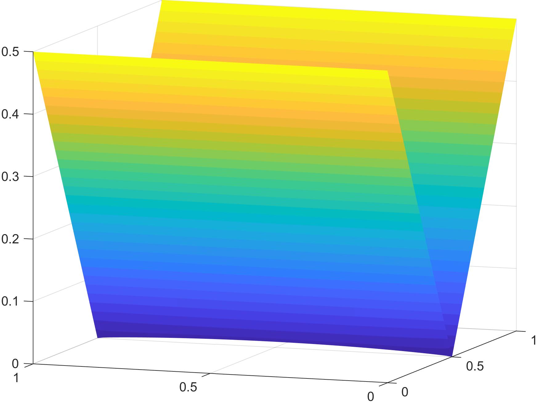
Figure 3. Discrete solution on a uniform mesh with 4225 nodes.

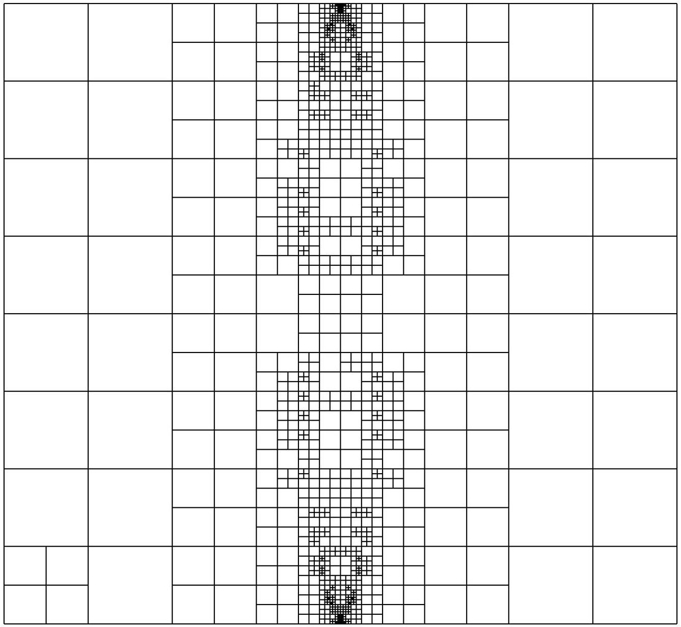
Figure 4. Adaptive mesh with 1907 nodes for the second experiment.

5.4. Nonsmooth exact solution

In this example, the function

$$u(x,y)\coloneqq-\big{(}\sin(\pi x)^{-1}+\sin(\pi y)^{-1}\big{)}^{-1}$$

is the solution to the Monge–Ampère equation (1.1) with homogenous boundary data and right-hand side

$$f(x,y)=\frac{4\pi^{2}\sin(\pi x)^{2}\sin(\pi y)^{2}(2-\sin(\pi x)\sin(\pi y))}{(\sin(\pi x)+\sin(\pi y))^{4}}.$$

The function $u$ belongs to $C^{2}(\Omega)\cap H^{2-\delta}(\Omega)$ for all $\delta>0$, but neither to $H^{2}(\Omega)$ nor $C^{2}(\overline{\Omega})$. The convergence history is displayed in Figure 5. Notice from Proposition 4.3 that $\mathrm{RHS}_{0}$ consists solely of the error in the Monge–Ampère measures. In this example, $f$ exhibits strong oscillations at the four corners of the domain $\Omega$ and the adaptive algorithm seems to solely refine towards these corners as displayed in Figure 6. While $\mathrm{RHS}_{0}$ converges on uniform meshes (although with a slow rate), there is only a marginal reduction of $\mathrm{RHS}_{0}$ for adaptive computation. We can conclude that the discrete approximation cannot resolve the infinitesimal oscillation of the Monge–Ampère measure of $u$ properly. This results in the stagnation of $\|u-u_{h,\varepsilon}\|_{L^{\infty}(\Omega)}$ and $\mathrm{LHS}$ at an early level in comparison to uniform mesh refinements. However, we also observed that the stagnation point depends on the maximal mesh-size. In fact, if we start from an initial uniform mesh with a small mesh-size $h_{0}$, significant improvements of $\mathrm{RHS}_{0}$ are obtained on the first levels of adaptive mesh refinements as displayed in Figure 7. Undisplayed experiments show the same behaviour for $\|u-u_{h,\varepsilon}\|_{L^{\infty}(\Omega)}$. This leads us to believe that, in this example, a combination of uniform and adaptive mesh-refining strategy provides the best results.

Figure 5. Convergence history for the third experiment with $\varepsilon=10^{-4}$.

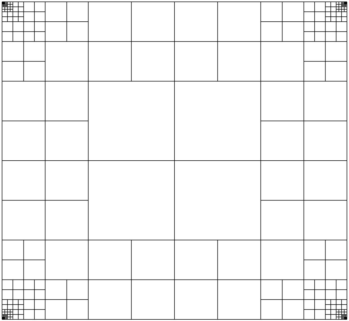
Figure 6. Adaptive mesh with 1351 nodes for the third experiment.

Figure 7. Convergence history of $\mathrm{LHS}$ for the third experiment with $\varepsilon=10^{-4}$ and different initial meshes.

References

- [1] A. D. Alexandrov, Dirichlet’s problem for the equation i, Vestnik Leningrad. Univ. Ser. Mat. Meh. Astr. 13 (1958), no. 1, 1–25.
- [2] C. Bradford Barber, David P. Dobkin, and Hannu Huhdanpaa, The quickhull algorithm for convex hulls, ACM Trans. Math. Software 22 (1996), no. 4, 469–483. MR 1428265
- [3] L. Caffarelli, M. G. Crandall, M. Kocan, and A. Święch, On viscosity solutions of fully nonlinear equations with measurable ingredients, Comm. Pure Appl. Math. 49 (1996), no. 4, 365–397. MR 1376656
- [4] Luis A. Caffarelli, Interior estimates for solutions of the Monge-Ampère equation, Ann. of Math. (2) 131 (1990), no. 1, 135–150. MR 1038360
- [5] Luis A. Caffarelli and Xavier Cabré, Fully nonlinear elliptic equations, American Mathematical Society Colloquium Publications, vol. 43, American Mathematical Society, Providence, RI, 1995. MR 1351007
- [6] Philippe G. Ciarlet, The finite element method for elliptic problems, Studies in Mathematics and its Applications, vol. 4, North-Holland, Amsterdam, 1978.
- [7] Michael G. Crandall, Hitoshi Ishii, and Pierre-Louis Lions, User’s guide to viscosity solutions of second order partial differential equations, Bull. Amer. Math. Soc. (N.S.) 27 (1992), no. 1, 1–67. MR 1118699
- [8] Guido De Philippis and Alessio Figalli, Second order stability for the Monge-Ampère equation and strong Sobolev convergence of optimal transport maps, Anal. PDE 6 (2013), no. 4, 993–1000. MR 3092736
- [9] E. J. Dean and R. Glowinski, Numerical methods for fully nonlinear elliptic equations of the Monge-Ampère type, Comput. Methods Appl. Mech. Engrg. 195 (2006), no. 13-16, 1344–1386.
- [10] Xiaobing Feng and Max Jensen, Convergent semi-Lagrangian methods for the Monge-Ampère equation on unstructured grids, SIAM J. Numer. Anal. 55 (2017), no. 2, 691–712. MR 3623696
- [11] Alessio Figalli, The Monge-Ampère equation and its applications, Zurich Lectures in Advanced Mathematics, European Mathematical Society (EMS), Zürich, 2017. MR 3617963
- [12] D. Gallistl and N. T. Tran, Convergence of a regularized finite element discretization of the two-dimensional Monge–Ampère equation, Math. Comp. (2022), Accepted for publication, arXiv:2112.10711.
- [13] Cristian E. Gutiérrez, The Monge-Ampère equation, Progress in Nonlinear Differential Equations and their Applications, vol. 89, Birkhäuser/Springer, [Cham], 2016, Second edition [of MR1829162]. MR 3560611
- [14] N. V. Krylov, Nonlinear elliptic and parabolic equations of the second order, Mathematics and its Applications (Soviet Series), vol. 7, D. Reidel Publishing Co., Dordrecht, 1987, Translated from the Russian by P. L. Buzytsky [P. L. Buzytskiĭ]. MR 901759
- [15] A. Maugeri, D. K. Palagachev, and L. G. Softova, Elliptic and parabolic equations with discontinuous coefficients, Wiley-VCH Verlag Berlin GmbH, Berlin, 2000.
- [16] R. Tyrrell Rockafellar, Convex analysis, Princeton Mathematical Series, No. 28, Princeton University Press, Princeton, N.J., 1970. MR 0274683
- [17] M. V. Safonov, Classical solution of second-order nonlinear elliptic equations, Izv. Akad. Nauk SSSR Ser. Mat. 52 (1988), no. 6, 1272–1287, 1328. MR 984219
- [18] Iain Smears and Endre Süli, Discontinuous Galerkin finite element approximation of nondivergence form elliptic equations with Cordès coefficients, SIAM J. Numer. Anal. 51 (2013), no. 4, 2088–2106. MR 3077903
- [19] by same author, Discontinuous Galerkin finite element approximation of Hamilton-Jacobi-Bellman equations with Cordes coefficients, SIAM J. Numer. Anal. 52 (2014), no. 2, 993–1016. MR 3196952