POD-mode-augmented wall model and its applications to flows at non-equilibrium conditions

Abstract

Insights gained from modal analysis are invoked for predictive large-eddy simulation (LES) wall modeling. Specifically, we augment the law of the wall (LoW) by an additional mode based on a one-dimensional proper orthogonal decomposition (POD) applied to a 2D turbulent channel. The constructed wall model contains two modes, i.e., the LoW mode and the POD-based mode, and the model matches with the LES at two, instead of one, off-wall locations. To show that the proposed model captures non-equilibrium effects, we perform a-priori and a-posteriori tests in the context of both equilibrium and non-equilibrium flows. The a-priori tests show that the proposed wall model captures extreme wall-shear stress events better than the equilibrium wall model. The model also captures non-equilibrium effects due to adverse pressure gradients. The a-posteriori tests show that the wall model captures the rapid decrease and the initial decrease of the streamwise wall-shear stress in channels subjected to suddenly imposed adverse and transverse pressure gradients, respectively, both of which are missed by currently available wall models. These results show promise in applying modal analysis for turbulence wall modeling. In particular, the results show that employing multiple modes helps in the modeling of non-equilibrium flows.

1 Introduction

The strict near-wall grid resolution requirements for large-eddy simulations (LES) make wall modeling a necessity at high Reynolds numbers (Choi & Moin, 2012; Yang & Griffin, 2021). The basic concept of wall-modeled LES (WMLES) is shown in schematic form in figure 1(a). As the LES grid in WMLES is coarse and scales with the boundary-layer thickness, the wall-shear stress and wall-heat flux cannot be computed per the discretization scheme. Instead, a wall model is employed. It takes LES information in the wall-adjacent cell(s) and computes the wall-shear stress and wall-heat flux. These wall fluxes are then used as Neumann boundary conditions at the wall in the LES.

The most extensively used type of wall model is the equilibrium wall models (EWMs) (Schumann, 1975; Bou-Zeid et al., 2005; Kawai & Larsson, 2012; De Vanna et al., 2021). The algebraic variant of EWMs computes the wall fluxes according to some mean flow scaling in the wall-adjacent computational cell(s) which is usually taken as the law of the wall (LoW). The mean flow scaling is matched with the LES velocity at an off-wall location locally and instantaneously, resulting in algebraic equations for the friction velocity and the friction temperature. The wall fluxes are then computed based on these friction quantities. Another popular variant of EWMs is based on solving the thin boundary-layer equations (TBLEs). In these models, only the Reynolds stress term and the viscous stress term are retained in the TBLEs, and the Reynolds stress term is closed using a zero-equation eddy viscosity model (Kawai & Larsson, 2012; Yang & Lv, 2018; Chen et al., 2022). The resulting ordinary differential equations (ODEs) are then solved on a 1D fine near-wall grid with the off-wall boundary condition provided by matching with the LES in the wall-adjacent cell(s). The wall fluxes can then be calculated from the ODE solutions on the wall model grid.

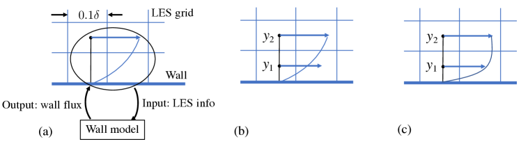
Figure 1: (a) Schematic of WMLES. (b) Schematic of the equilibrium wall model (EWM). Here, the wall model (WM) and the LES match at the second off-wall grid point. (c) Schematic of the POD-augmented WM. The WM and the LES match at two off-wall grid points.

Although the EWMs discussed above have much in their favor regarding simplicity, model stability, and a low computational cost, it has long been known that EWMs struggle in non-equilibrium flows, and thus, improvements in wall modeling beyond the EWMs are needed (Piomelli & Balaras, 2002; Larsson et al., 2016; Bose & Park, 2018). In the following, we review a few recent approaches. One approach is based on solving the full TBLEs with all of the non-equilibrium terms included (Park & Moin, 2014). This method, however, comes at the cost of solving a full set of partial differential equations (PDEs), which often adds a 100% overhead to the LES as in Park & Moin (2016). Approaches that account for non-equilibrium effects at a lower computational cost are the integral wall model (IWM) by Yang et al. (2015) and the Lagrangian relaxation towards equilibrium wall model (LaRTE) by Fowler et al. (2022). Both models perform wall-normal integration of the full TBLEs with an assumed analytical form for the LES-grid filtered velocity. This results in a wall model that only requires the solution of algebraic equations. Another interesting wall modeling approach is the dynamic slip wall model (Bose & Moin, 2014; Bae et al., 2019). In this approach, a slip boundary condition is derived from the filtered Navier-Stokes equations, which is then used instead of the traditional Neumann boundary condition at the wall.

We consider boundary layers subjected to adverse and transverse pressure gradients, which remain challenges for wall modeling (Bose & Park, 2018). Adverse pressure gradients (APGs) and transverse pressure gradients (TPGs) arise in many flows (Monty et al., 2011; Volino, 2020; Goc et al., 2021). For the present work, we focus on the model problem shown in figure 2(a, b) where a 2D channel is subjected to a suddenly imposed pressure gradient (Na & Moin, 1998; He & Seddighi, 2015; Lozano-Durán et al., 2020), here, a suddenly imposed APG or TPG. The flow decelerates in (a) and changes direction in (b). Relevant to near-wall turbulence modeling efforts is the behavior of the mean flow, which is the input to a wall model, and the wall-shear stress, which is the output of a wall model. Figure 2(c) shows the evolution of the mean flow in (a) after an APG $f_{x}=100f_{x,0}$ is suddenly imposed to a $Re_{\tau}=1000$ channel. Here $Re_{\tau}=u_{\tau}\delta/\nu$ with $u_{\tau}$ the friction velocity, $\delta$ is the half-channel width, and $\nu$ is the kinematic viscosity. The mean velocity profile in inner units is above the LoW, and if one were to apply the LoW to predict the wall-shear stress, the wall-shear stress would be grossly over-predicted. Figure 2(d) shows the evolution of the $x$-direction wall-shear stress, $\tau_{x}$, after a TPG $f_{z}=10f_{x,0}$ is applied to a $Re_{\tau}=1000$ channel. The wall-shear stress decreases initially and then increases. This behavior, however, is not captured by the available wall models.

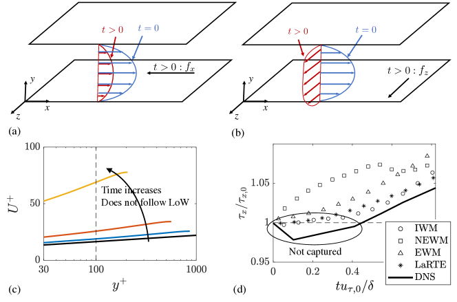
Figure 2: Schematics of a 2D channel subjected to (a) a suddenly imposed APG and (b) a suddenly imposed TPG at $t=0$. Here, $f_{x}$ and $f_{z}$ are the imposed pressure gradients in the $x$ and $z$ directions, $t$ is the time, $x$, $y$, and $z$ are the three Cartesian coordinates. (c) Evolution of the velocity profiles in time after an APG $f_{x}=100f_{x,0}$ is suddenly applied to a $Re_{\tau}=1000$ channel. The solid black line corresponds to the log law $U^{+}=\log(y^{+})/\kappa+B$, where $\kappa=0.4$ and $B=5$. Here, $u_{\tau}$ is the friction velocity, $f_{x,0}$ is the driving force of the 2D channel, $U$ is the streamwise velocity, and the superscript $+$ denotes normalization by wall units. (d) Evolution of the $x$-direction wall-shear stress after a TPG $f_{z}=10f_{x,0}$ is applied to a $Re_{\tau}=1000$ channel. DNS: direct numerical simulation (Lozano-Durán et al., 2020), IWM: integral wall model (Yang et al., 2015), NEWM: non-equilibrium wall model (Park & Moin, 2014), EWM: equilibrium wall model (Yang et al., 2017), and LaRTE: Lagrangian relaxation towards equilibrium wall model (Fowler et al., 2022).

This work aims to advance WMLES by accounting for the aforementioned non-equilibrium effects. The idea is to augment the LoW such that the ansatz used for velocity reconstruction in the wall-adjacent cell(s) provides a more realistic description of the LES-grid-filtered flow than the LoW. First, however, we briefly review algebraic EWMs based on the LoW to establish some context. In these models, the following ansatz is used for the near-wall flow

$${\bf U}={\bf c}{\rm LoW}(y^{+})\,,$$ (1)

where ${\bf U}=(U,W)$ are the wall-parallel velocities at a distance $y$ from the wall, ${\rm LoW}(y^{+})$ is usually taken to be the logarithmic law of the wall, and $y^{+}=(u_{\tau}/\nu)y$ is the wall-unit-scaled distance from the wall. We will take ${\rm LoW}(y^{+})$ to include the viscous sublayer, the buffer layer, and the logarithmic layer, but not the wake layer. Further, ${\rm LoW}(y^{+})$ is taken to be nondimensional such that the friction velocity $u_{\tau}$ has been absorbed into the coefficients. We propose to generalize these models by employing the augmented ansatz

$${\bf U}={\bf c}_{1}{\rm LoW}(y^{+})+{\bf c}_{2}g(y^{+})\,,$$ (2)

where $g(y^{+})$ is, at this point, a generic nondimensional function. Figure 1(b, c) is a schematic of the velocity reconstruction according to (1) and (2), respectively. Inclusion of the function $g$ gives the wall model in figure 1(c) the ability to account for deviations from the LoW scaling, and thus, to respond to both instantaneous fluctuations and non-equilibrium effects. For convenience, we will refer to both of these cases as capturing non-equilibrium effects. Yang et al. (2015) and Lv et al. (2021) argued that $g\sim y$ to leading order, but other choices that more closely mimic the physics of wall-bounden turbulent flows could yield better results. To that end, we propose to obtain $g$ from modal analysis of the near-wall region of a 2D turbulent channel as a starting point for such investigations. While many possible choices are available today (Taira et al., 2017), we invoke the proper orthogonal decomposition (POD) given its physical underpinning (the fact that POD modes capture most energy) and its historically important role in near-wall turbulence modeling (Aubry et al., 1988; Berkooz et al., 1993). Specifically, the mode $g$ is constructed based on a one-dimensional scalar variant of POD which is performed on the fluctuating streamwise velocity component (i.e., with the LoW subtracted) along the wall-normal direction.

The remainder of this work is organized as follows. In §2, we provide further details of the proposed wall model including a discussion of how the $g$ mode is constructed. In §3, we present results of an a-priori analysis of a 2D turbulent channel and a channel subjected to suddenly imposed APGs. In §4, a-posteriori test results are presented, again including a 2D turbulent channel and a channel with suddenly imposed APGs. We also consider a channel with a suddenly imposed TPG. Finally, in §5, the conclusions arrived at in this work are presented.

2 Methodology

2.1 Wall model formalism

We start by considering algebraic EWMs to provide some context for our proposed extension. In these models, we employ the LoW ansatz in (1) as an approximation of the near-wall flow. This is done by matching the LoW locally with the wall-parallel LES velocities such the LoW is applied along the local streamwise direction. As equation (1) has only one mode, i.e., the LoW mode, we can determine the coefficients ${\bf c}=(c_{x},c_{z})$ from matching information at a single off-wall location. This gives the equations

$$c_{x}{\rm LoW}(y^{+})=U\,,\quad c_{z}{\rm LoW}(y^{+})=W\,,$$ (3)

where $y^{+}$ is the wall-unit-scaled height of the matching location while $U$ and $W$ are the local wall-parallel LES velocities at this height. We can then calculate the wall-shear stress ${\boldsymbol{\tau}_{w}}=(\tau_{x},\tau_{z})$ from (1) as follows

$${\boldsymbol{\tau}_{w}}=\nu\left.\frac{d{\bf U}}{dy}\right|_{y=0}=\nu{\bf c}\left.\frac{d{\rm LoW}}{dy^{+}}\right|_{y=0}\left.\frac{dy^{+}}{dy}\right|_{y=0}={\bf c}u_{\tau}\,,$$ (4)

where we have used that $dy^{+}/dy=u_{\tau}/\nu$ and $\left.d{\rm LoW}/dy^{+}\right|_{y=0}=1$ by definition. To relate the friction velocity $u_{\tau}$ to the coefficients ${\bf c}$, we note that EWMs assume a local state of equilibrium. The wall-shear stress amplitude is therefore given by $\tau_{w}=|\boldsymbol{\tau}_{w}|=u_{\tau}^{2}$. This, together with (4), gives the following relation

$$u_{\tau}=(c_{x}^{2}+c_{z}^{2})^{1/2}\,.$$ (5)

Thus, the appearance of the friction velocity in (3) (contained in $y^{+}$) results in this being a nonlinear set of equations that would require an iterative method to obtain the solution. However, this requirement can be removed by using $u_{\tau}$ from the previous time step or from long-time averaging. In this case, (3) can be solved directly and (4) is then invoked to calculate the wall-shear stress.

The proposed extension in (2), on the other hand, has two modes, i.e., LoW and $g$. To determine the coefficients ${\bf c}_{1}=(c_{1x},c_{1z})$ and ${\bf c}_{2}=(c_{2x},c_{2z})$, matching with the LES at two off-wall locations is used

$$\begin{split}&c_{1x}{\rm LoW}(y_{1}^{+})+c_{2x}g(y_{1}^{+})=U_{1}\,,\quad c_{1z}{\rm LoW}(y_{1}^{+})+c_{2z}g(y_{1}^{+})=W_{1}\,,\\ &c_{1x}{\rm LoW}(y_{2}^{+})+c_{2x}g(y_{2}^{+})=U_{2}\,,\quad c_{1z}{\rm LoW}(y_{2}^{+})+c_{2z}g(y_{2}^{+})=W_{2}\,.\end{split}$$ (6)

Here, $y_{1}^{+}$ and $y_{2}^{+}$ are the wall-unit-scaled heights of the two matching locations while $U_{1,2}$ and $W_{1,2}$ are the local wall-parallel LES velocities at these heights. Note that similar to EWMs, the augmented LoW ansatz is applied along the local streamwise direction. The wall-shear stress ${\boldsymbol{\tau}}_{w}=(\tau_{x},\tau_{z})$ can then be calculated similar to the EWM as

$${\boldsymbol{\tau}}_{w}=\nu\left.\frac{d{\bf U}}{dy}\right|_{y=0}=\nu\left({\bf c}_{1}\left.\frac{d{\rm LoW}}{dy^{+}}\right|_{y=0}+{\bf c}_{2}\left.\frac{dg}{dy^{+}}\right|_{y=0}\right)\left.\frac{dy^{+}}{dy}\right|_{y=0}=({\bf c}_{1}+{\bf c}_{2})u_{\tau}\,,$$ (7)

where we have again used that $dy^{+}/dy=u_{\tau}/\nu$ and $\left.d{\rm LoW}/dy^{+}\right|_{y=0}=1$, while $\left.dg/dy^{+}\right|_{y=0}=1$ is enforced through normalization of $g$. Further, as for EWMs, we assume that the wall-shear stress magnitude can be expressed through a local friction velocity such that $\tau_{w}=|{\boldsymbol{\tau_{w}}}|=u_{\tau}^{2}$ still holds for the proposed model. Using this assumption, together with (7), we get

$$u_{\tau}=\left[\left(c_{1x}+c_{2x}\right)^{2}+\left(c_{1z}+c_{2z}\right)^{2}\right]^{1/2}\,.$$ (8)

Comparing with the EWM result from (5), we see that the structure is very similar. Further, the friction velocity $u_{\tau}$ in (6) (contained in $y_{1}^{+},y_{2}^{+}$) results in a set of nonlinear equations, which can be handled in the same way as for the EWM. With the coefficients determined, (7) is then invoked to compute the wall-shear stress. It is worth noting that the model reduces to an algebraic EWM when ${\bf c}_{2}=0$.

Following Yang et al. (2017), we apply additional filtration to the velocities at both matching locations. This filtration allows us to place the matching location(s) close to the wall without a log-layer mismatch, which is preferred to placing the matching location(s) further away; since the latter incurs penalties on parallel computing, among other disadvantages. Yang et al. (2017) also found similar behaviors using temporal and spatial filters in 2D channel flow cases. We have chosen to only consider spatial filtering in this work since the model will be validated against highly unsteady flows, for which spatial filtering is more appropriate.

2.2 Wall model modes

We now describe the two modes, i.e., ${\rm LoW}$ and $g$, in greater detail. The construction of the $g$ mode is covered separately in §2.3 below, and we discuss the effect of the choice of the $g$ mode in Appendix B. Figure 3(a) shows the LoW mode. This is straightforward. The mode contains the viscous sublayer, the buffer layer, and the logarithmic layer, but not the wake layer. The behavior of the LoW mode conforms to $U^{+}=\log(y^{+})/\kappa+B$ at sufficiently large $y^{+}$. Analytical expressions for the viscous sublayer and buffer layer can be found in Reichardt (1951) and Spalding (1961). Figure 3(b) shows the POD-based mode $g$. The mode is approximately constant away from the wall and conforms to the no-slip condition at the wall.

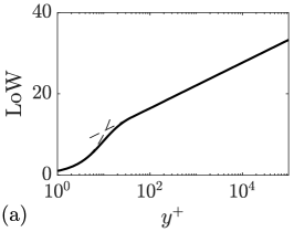
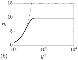
Figure 3: (a) The LoW mode. The two dashed lines correspond to ${\rm LoW}=y^{+}$ and ${\rm LoW}=\log(y^{+})/\kappa+B$. (b) The $g$ mode. The two dashed lines correspond to $g=y^{+}$ and $g=9.7$.

A basic requirement of a wall model is that it degenerates to the no-slip condition at the wall-resolved limit. Here, We discuss the behavior of the model when the viscous sublayer is resolved. When the viscous layer is resolved, we have

$${\bf U}=\left.\frac{d{\bf U}}{dy}\right|_{y=0}y\,,$$ (9)

at first off-wall grid points. As seen in figure 3, both the LoW and the mode $g$ are linear functions of $y^{+}$ in the viscous sublayer, so in this case, we have

$${\rm LoW}=g=y^{+}\,.$$ (10)

It follows from (9) and (10) that (6) reduces to

$$({{\bf c}_{1}+{\bf c}_{2}})y_{1}^{+}=\left.\frac{d{\bf U}}{dy}\right|_{y=0}y_{1}\,,\quad({{\bf c}_{1}+{\bf c}_{2}})y_{2}^{+}=\left.\frac{d{\bf U}}{dy}\right|_{y=0}y_{2}\,.$$ (11)

The two equations have the following solution

$${{\bf c}_{1}+{\bf c}_{2}}=\frac{\bf U}{|{\bf U}|}u_{\tau}\,.$$ (12)

Although ${\bf c}_{1}$ and ${\bf c}_{2}$ are not uniquely determined, ${{\bf c}_{1}+{\bf c}_{2}}$ is. As a result, the wall-shear stress is uniquely determined. We also notice that (12) is non-singular even when the wall-shear stress is 0. Hence, $\tau_{w}=0$ is a removable singularity ($\tau_{w}=0$ is a singularity because $y^{+}$ is not defined when $\tau_{w}=0$, it is removable because it does not create any mathematical singularity to the calculation of the wall-shear stress). In terms of numerical implementation, one could choose to do a minimum norm solution, which would be quite elegant. We have chosen to add a simple “if” statement that allows the code to treat wall-resolved grids separately.

Finally, when implementing the wall model, we tabulate the LoW mode and the $g$ mode in a lookup table. An inquiry about LoW’s and $g$’s values at a given $y^{+}$ is then interpolated from the lookup table. Here, we prefer lookup tables over analytical formulation because “addressing” a lookup table is more efficient than computing a closed-form expression. In computer science terms, a lookup table is an array that replaces runtime computation with a simpler array indexing operation. The tables may be precalculated and stored in static program storage, pre-fetched as part of a program’s initialization, or stored in hardware in application-specific platforms. The process is called “direct addressing”. Because retrieving a value from memory is often faster than carrying out a more expensive computation or input/output operation, lookup tables can save processing time.

2.3 Construction of the g mode

Define ${\bf r}={\bf U}-{\bf c}_{1}{\rm LoW}$ such that ${\bf r}=(r_{x},r_{z})$ describes the deviation from the LoW. The $g$ mode, or more precisely ${\bf c}_{2}g$, is intended to capture ${\bf r}$. Any function, as long as it is not exactly the LoW, should capture part of that deviation. Here, we want a mode that captures as much energy in $\bf r$ as possible. This directly leads to POD. Specifically, we consider a one-dimensional scalar variant of POD. It is POD of the fluctuating streamwise velocity component along the wall-normal direction in a 2D turbulent channel. Further details on the numerical implementation are given in Appendix A. As POD can be performed in multiple spatial dimensions, we provide a few observations in this regard. First, if the POD analysis were to be performed in 3D space, a local coupling between the wall model and LES would no longer be possible. Instead, a more global coupling over some wall-parallel plan(s) would be necessary which could be limiting for flows in complex geometries. Second, a global coupling between LES and the wall model could be problematic in the parallelization of the WMLES code.

We perform this one-dimensional POD for wall-normal intervals ranging from the wall to the log-layer region in a 2D turbulent channel with $Re_{\tau}=5200$ (Lee & Moser, 2015). Three different heights within the log-layer are considered. The result for the first POD mode is shown in figure 4. We see that the near-wall part of the POD mode does not change and that the modes asymptote to a constant in the logarithmic layer. This gives rise to the $g$ mode in figure 3(b). Further, the POD spectra for the three different analyses are given in figure 5. In figure 5(a), it can be observed that the first and second POD modes carry roughly 50% and 15% of the total energy, respectively, for all three cases. This shows that the first POD mode is significantly more important than the subsequent modes. It is curious to note that the $g$ mode used here is almost identical to the laminar mode in Fowler et al. (2022), where the mode describes the response of the flow to an alternating pressure gradient. This suggests that the instantaneous flow in an equilibrium channel is also subjected to large instantaneous pressure gradients.

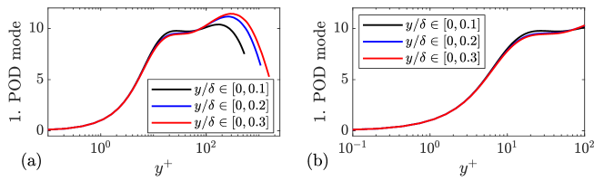
Figure 4: (a) First POD mode for three wall-normal intervals which start from the wall and end at $y/\delta=0.1$, $0.2$, and $0.3$. (b) Zoom in on the near-wall region.

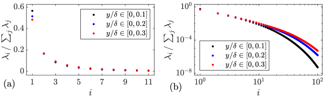
Figure 5: (a) POD eigenvalue spectra for the three cases in figure 4. (b) Same as in (a) but in a double logarithmic plot.

We also comment on the choice of $Re_{\tau}=$5200 for the POD analysis. As WMLES is primarily aimed at high Reynolds number flows, it is preferable to base the POD analysis on such a case. Currently, $Re_{\tau}=5200$ is the largest Reynolds number for which the instantaneous velocity field, needed for the POD analysis, is publicly available (Graham et al., 2016). Still, an ideal wall model should be able to perform well also at low Reynolds numbers. Therefore, we have performed a simple test at different $Re_{\tau}$ for both the EWM (1) and POD-augmented WM (2), with the $g$ mode from $Re_{\tau}=5200$ in figure 3(b), to compare them in terms of capturing the turbulent kinetic energy (TKE). We do this using DNS data from four different Reynolds numbers: $Re_{\tau}=180$, 540, 1000, and 5200. The data for the two cases $Re_{\tau}=180$ and $540$ are generated using a code with the same numerics as in Kim et al. (1987) while the cases $Re_{\tau}=1000$ and 5200 are from Lee & Moser (2015); Graham et al. (2016). We then fit the streamwise coefficients of both wall models in (1) and (2) by a least squares regression using the streamwise velocity from DNS data over the interval $0\leq y/\delta\leq 0.1$. This interval is chosen to be consistent with the subsequent a-priori and a-posteriori testing for a 2D turbulent channel in §3 and §4, respectively. The results are shown in figure 6. We observe that the POD-augmented WM captures significantly more of the TKE than the EWM at all Reynolds numbers considered. In regards to the decrease in the captured TKE with increasing Reynolds number, which is observed for both wall models, this can be explained by analogy with the momentum cascade in homogeneous isotropic turbulence. Specifically, as the Reynolds number increases, smaller and smaller scales are activated in the flow which then start contributing to the total TKE. As these small scales cannot be captured by a few large-scale modes, the relative fraction of the TKE captured by such a finite set of large-scale modes will inevitably decrease as the Reynolds number increases.

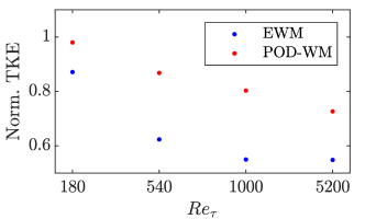
Figure 6: Normalized streamwise TKE captured by the EWM in (1) and POD-augmented WM in (2) for different $Re_{\tau}$. The normalization is by the TKE from DNS.

Admittedly, the POD modes in another flow will not be the same as the ones in a 2D channel, but we argue that this is not a huge concern here given the purposes of this work. Specifically, considering POD modes from other wall-bounded turbulent flows will only be meaningful if the present approach yields more accurate results than the EWM. If this turns out to be the case, a more detailed analysis involving POD modes from other flows should be considered to determine the potential benefits of using particular modes in different flow types. Still, we note that the flow physics that governs the instantaneous flow in a channel is also present in other wall-bounded flows. Therefore, wall modeling improvements based on a mode from this case would be an encouraging sign for application in other flow types as well. Last, we comment on the choice of the flow configuration. Considering that the inner layer of a boundary layer is no different from that of a channel, POD analysis of a boundary-layer flow should give us similar results. Nonetheless, DNS data of channel flows is more extensively available than DNS data of boundary layers.

3 A-priori analysis

We perform a comparative a-priori analysis between the EWM and the POD-augmented WM. We consider a 2D equilibrium channel and channels subjected to a strong adverse pressure gradient. We will show that the present POD-augmented WM captures non-equilibrium effects more accurately than the EWM.

3.1 Equilibrium channel

We consider a 2D turbulent channel with $Re_{\tau}=1000$ (Graham et al., 2016). We filter the DNS data following Graham et al. (2016) and Yang et al. (2019) so that the study is more faithful to WMLES than DNS. A Gaussian filter is used with a filtration length scale of $300(\nu/u_{\tau})$. This length scale is chosen to match the grid resolution used in the subsequent a-posteriori investigations in §4.2 to make the results more comparable. The filtered DNS data is then used to fit for the coefficients in (1) and (2). Note that we use the same DNS data for fitting both the EWM and POD-WM to ensure a fair comparison. Specifically, the matching locations are at $y/\delta=0.5/12$ and 1.5/12, i.e., the first and the second off-wall grid point locations in the subsequent a-posteriori study in §4.2. The wall-shear stress is computed according to (4) for the EWM and (7) for the POD-augmented WM. The wall-shear stress computed from the EWM and POD-augmented WM is compared with the wall-shear stress from both DNS and filtered DNS in figure 7. We observe the following. First, both the EWM and POD-augmented WM predict the correct mean stress. Second, the EWM captures the large-scale variations of the wall-shear stress, but it does not capture the more extreme wall-shear stress events. On the other hand, the POD-augmented WM captures the large-scale variation and some of the extreme events. For a more quantitative comparison, we note that the root-mean-square (rms) of the wall-shear stress fluctuations $\tau_{w,{\rm rms}}^{+}$ is 0.42, 0.13, 0.11, and 0.20 in DNS, filtered DNS, predicted by the EWM, and predicted by the POD-augmented WM, respectively. Further, we also give the rms of the error between the filtered DNS and the EWM and POD-WM predictions which are 0.09 and 0.16, respectively. Thus, we see that the rms of the error is larger for the POD-augmented WM than the EWM when the models are compared with filtered DNS data. As the POD-augmented WM contains two modes, i.e., the LoW and POD-based mode $g$, it is interesting to investigate the behavior of the coefficients in front of these two modes. Figure 8 shows the contours of these coefficients and their correlation. First, we observe that the two coefficients are of the same magnitude. Second, there is a strong anti-correlation between the LoW mode and the $g$ mode coefficients. This suggests that when the equilibrium LoW term deviates from the mean value, the non-equilibrium term pulls it back. We have repeated the above a-priori test at other Reynolds numbers and matching locations. We see that $c_{1x}$ and $c_{2x}$ are always anti-correlated, but the correlation depends on the Reynolds number and the matching location. The exact physical mechanism behind this observation is not entirely clear to us, but this phenomenon, if it translates to WMLES, will help to stabilize the numerical simulation.

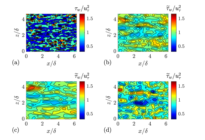
Figure 7: (a) Wall-shear stress from DNS. (b) Wall-shear stress from filtered DNS.
(c) Wall-shear stress predicted by the EWM. (d) Wall-shear stress predicted by the POD-augmented WM. The WM calculations are discussed in the text. Note that we show only part of the computational domain for presentation purposes.

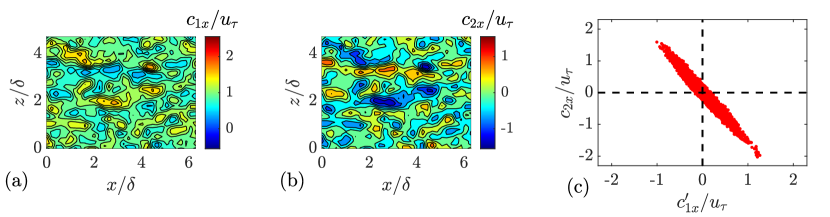
Figure 8: (a) Contours of $c_{1x}$. (b) Contours of $c_{2x}$. (c) Instantaneous realizations of $c_{1x}^{\prime}$ and $c_{2x}$.

3.2 Non-equilibrium channel

The main purpose of the POD-augmented WM is to capture non-equilibrium effects that are not captured by the EWM. In this subsection, we consider the time-evolution of a 2D channel flow subjected to suddenly applied APGs. Using the nomenclature R[$Re_{\tau}$]A[APG$/(\tau_{w,0}/\delta)$], we consider the two cases: R1000A10 and R1000A100 with moderate and strong adverse pressure gradients. Again, we fit for the coefficients in (1) and (2) using the same matching information for both models with the matching locations being the same as those used in the a-posteriori study in §4.3. The wall-shear stress is computed according to (4) and (7). We then compare the computed wall-shear stresses to the DNS.

Figure 9(a, b) shows the R1000A10 results. We see from figure 9(a) that there is a good agreement between the LoW coefficients $c_{x}$ and $c_{1x}$ from the EWM and POD-augmented WM, respectively, and that the $g$ mode in the POD-augmented WM is almost entirely “turned off” as $c_{2x}\approx 0$. Hence, the POD-augmented WM formulation reduces to the EWM in near-equilibrium conditions. In regards to the accuracy of the wall-shear stress predictions, we see that both the EWM and POD-augmented WM produce accurate results as seen in figure 9(b). Still, it should be observed that the POD-augmented WM performs slightly worse than the EWM for this near-equilibrium case. Next, the R1000A100 results are shown in figure 9(c, d). From figure 9(c), we see that the LoW coefficients for the EWM and POD-augmented WM no longer agree and that the $g$ mode in the POD-augmented WM is active. Specifically, for the POD-augmented WM, we observe that the LoW coefficient $c_{1x}$ remains almost constant while the $g$ coefficient $c_{2x}$ continuously decreases. Further, the wall-shear stress predictions in figure 9(d) show that the POD-augmented WM does a much better job of capturing the strong decrease in the wall-shear stress than the EWM.

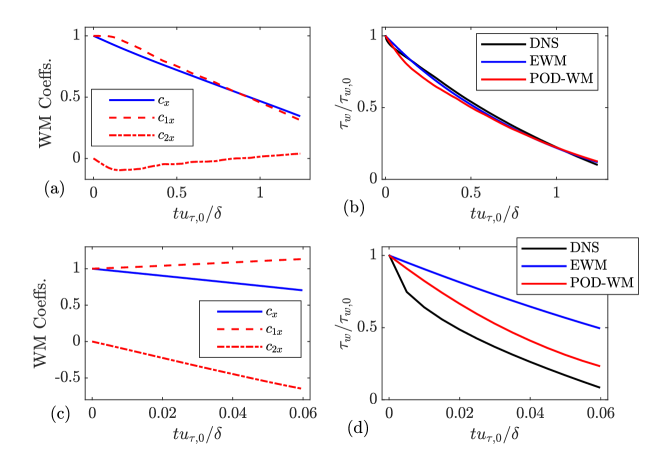
Figure 9: (a) WM coefficients $c_{x}$ from the EWM and $c_{1x}$ and $c_{2x}$ from the POD-augmented WM in the case R1000A10. (b) Wall-shear stress from DNS, the EWM, and the POD-augmented WM in case R1000A10. (c, d) Same as (a, b) but for case R1000A100.

4 A-posteriori studies

Good results in a-priori analysis do not necessarily translate to good results in a-posteriori studies. We apply the POD-augmented WM to an equilibrium 2D channel, and channels subjected to a suddenly imposed adverse or transverse pressure gradient.

4.1 Code

The POD-augmented WM is implemented in our in-house pseudo-spectral code LESGO. The code solves the incompressible Navier-Stokes equations in a half-channel with a slip top boundary and periodicity in both the streamwise and the spanwise directions. The flow is driven by a constant streamwise pressure gradient. The code employs a pseudo-spectral method in the streamwise and the transverse directions, a second-order finite difference method in the wall-normal direction, and the second-order Adam-Bashforth method for time stepping. The grid is uniform in each direction. The time step size is such that the CFL number is always smaller than 0.06 (due to the Adams-Bashforth time-stepping scheme). Further, a Gaussian filter is applied to the wall-parallel velocities before they are used as input to the wall model. Last, the sub-grid scale (SGS) stresses are modeled via the Lagrangian scale-dependent model (Bou-Zeid et al., 2005). The code is well-validated (Abkar & Moin, 2017; Yang et al., 2022) and further details of the code’s numerics can be found in Yang & Abkar (2018) and the references cited therein.

4.2 Fully developed channel

We first apply the POD-augmented WM in 2D equilibrium channels. This exercise will serve as validation: the WM must be able to predict the law of the wall at all Reynolds numbers on both wall-resolved and wall-modeled grids. Table 1 shows the details of the WMLES. The nomenclature of the cases is R[$Re_{\tau}$]N[$N_{y}$]. The Reynolds number is from $Re_{\tau}=180$ to $10^{5}$, the grid is from DNS-like (in case R180N48) to typical-WMLES-like (R1000N12, R1e5N12), and the domain is of the size as in Lozano-Durán & Jiménez (2014). The LES/WM matching locations are at the first two off-wall grid points, which are used by both wall models. The matching locations are in the viscous sublayer (in case R180N48) or the logarithmic layer (in cases R1000N12, R1e5N12, R1e5N24, R1e5N48). Following the established best practice (Larsson et al., 2016), the matching locations are not placed in the buffer layer. Placing the matching location within the buffer layer incurs log-layer mismatch for WMLES in general—even if the matching location is not the first off-wall grid point and the velocity at the matching location is filtered. Nonetheless, placing the matching location is rarely a concern for flows at high Reynolds numbers since the buffer layer will not be resolved. This issue comes up here only because we validate against DNS data, which is limited to moderate Reynolds numbers. Figure 10(a) shows the mean flow. The profiles follow the LoW irrespective of the grid and the Reynolds number. We see some difference at high Reynolds numbers when the grid resolution is low, which may be due to the interplay between the SGS model and the wall model. Figure 10(b, c) shows the instantaneous contours of $c_{1x}$ and $c_{2x}$. The mean flow is $U=u_{\tau}~{}{\rm LoW}(y^{+})$ in a channel. Hence, $c_{1x}$’s mean should be $u_{\tau}$ and $c_{2x}$’s mean should be $0$. The above expectation bears out in figure 10(b, c) where $c_{1x}/u_{\tau}=0.96$ and $c_{2x}/u_{\tau}=0.05$ when averaged over the wall-parallel directions. We note that the observed deviation from $c_{1x}=u_{\tau}$ and $c_{2x}=0$ is due to instantaneous effects as they disappear upon time averaging. Further, the local instantaneous deviations in $c_{1x}$ from $u_{\tau}$ is a result of non-equilibrium effects, where we should see the POD-based $g$ mode. This expectation also bears out in figure 10(b, c).

Case	$Re_{\tau}$	Grid	Domain	$\Delta y^{+}/2$	WM
R180N48	180	$96\times 48\times 96$	$2\pi\times 2\times\pi$	1.88	EWM, POD-augmented WM
R1000N12	1000	$24\times 12\times 24$	$2\pi\times 2\times\pi$	41.7	EWM, POD-augmented WM
R1e5N12	$10^{5}$	$24\times 12\times 24$	$2\pi\times 2\times\pi$	4.17$\times 10^{3}$	EWM, POD-augmented WM
R1e5N24	$10^{5}$	$48\times 24\times 48$	$2\pi\times 2\times\pi$	$2.08\times 10^{3}$	EWM, POD-augmented WM
R1e5N48	$10^{5}$	$96\times 48\times 96$	$2\pi\times 2\times\pi$	$1.04\times 10^{3}$	EWM, POD-augmented WM

Table 1: WMLES details. The half-channel height is used to normalize the numbers in the “Domain” column. The first off-wall grid point is at $\Delta y/2$ (the half is because of the staggered grid).

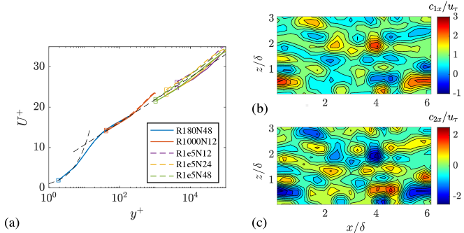
Figure 10: (a) Mean velocity profiles. The square symbols indicate the location of the first off-wall grid point. The solid lines are POD-WM results, and the dashed lines are EWM results. (b) Contours of $c_{1x}$. (c) Contours of $c_{2x}$.

4.3 Adverse pressure gradient

Next, we apply the POD-augmented WM in a channel subjected to a suddenly imposed APG. A schematic of the flow was shown in figure 2(a) already, and figure 2(c) shows the time evolution of the mean flow. Table 2 shows the WMLES details. The nomenclature is R[$Re_{\tau}$]A[APG$/(\tau_{w,0}/\delta)$], where the subscript 0 indicates a variable evaluated prior to the application of the APG. The channel is initially at a Reynolds number $Re_{\tau}=1000$. The APGs are 10$(\tau_{w,0}/\delta)$ and 100$(\tau_{w,0}/\delta)$ in cases R1000A10 and R1000A100, respectively. The flow decelerates, and the Reynolds number decreases. LES information at the second and the fourth off-wall grid points are fed to the POD-augmented WM so that we do not match in the buffer layer. For a fair comparison, the EWM makes use of the LES information at these two off-wall locations as well. Specifically, the EWM predicts wall-shear stress that yields the best fit of the velocity through the second and fourth off-wall grid points.

Case	$Re_{\tau,0}$	Grid	Domain	APG	WM
R1000A10N12	1000	$24\times 12\times 24$	$2\pi\times 2\times\pi$	10	EWM, POD-augmented WM
R1000A100N12	1000	$24\times 12\times 24$	$2\pi\times 2\times\pi$	100	EWM, POD-augmented WM

Table 2: WMLES details. The half-channel height is used to normalize the numbers in the “Domain” column. The APG column shows the magnitude of the suddenly imposed APG. The numbers are normalized using $\tau_{w,0}/\delta$.

Figure 11(a, b) shows the flow rate as a function of time for R1000A10 and R1000A100, respectively, and we compare WMLES and DNS. The DNS data are by the present authors as well. The setups are similar to those in He & Seddighi (2015) and are not detailed here for brevity. We see from figure 11(a, b) that the flow rate is accurately predicted irrespective of the wall model.

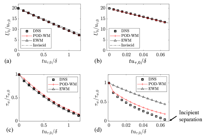
Figure 11: (a, b) Flow rate as a function of time. (a) R1000A10. (b) R1000A100. Here, “Inviscid” corresponds to (13). (c, d) Wall-shear stress as a function of time. (c) R1000A10. (d) R1000A100. DNS: values given by the DNS, which we take as the truth. POD-WM: predictions by the WMLES that employs the POD-augmented WM for near-wall turbulence modeling. EWM: predictions by the WMLES that employs the EWM for near-wall turbulence modeling.

We explain why wall modeling is not critical to the prediction of the flow rate and the velocity itself. The flow rate is governed by the following volume-integrated $x$ momentum equation, ${d(\rho U_{b})}/{dt}=-{\tau_{w}}/{\delta}-{dP}/{dx}$. If the flow is inviscid, this equation becomes ${d(\rho U_{b})}/{dt}=-{dP}/{dx}$, which directly leads to

$$U_{b}=U_{b,0}-\frac{1}{\rho}\frac{dP}{dx}t\,.$$ (13)

The above inviscid estimate is plotted in figure 11(a, b) and is fairly accurate. In fact, the imposed adverse pressure gradient overwhelms the wall-shear stress and dominates the evolution of the velocity field. This makes wall modeling less critical to the prediction of the flow rate.

A more difficult test is the wall-shear stress. Figure 11(c, d) shows the (horizontally averaged) wall-shear stress as a function of time for R1000A10 and R1000A100, respectively. The EWM captures the wall-shear stress in case R1000A10 but grossly over-predicts the wall-shear stress in case R1000A100. The POD-augmented WM, on the other hand, captures the wall-shear stress well in both cases—although its prediction becomes less accurate as the flow approaches separation in case R1000A100. We also observe that the POD-augmented WM is slightly less accurate than the EWM for the R1000A10 case which was also observed in the a-priori tests.

We have shown in §3 that the POD-augmented wall model captures non-equilibrium effects. Here, we explain why the POD-augmented WM is more accurate than the EWM. We note that the velocity and the wall-shear stress are coupled, and the accurate prediction of one depends on the accurate prediction of the other. Nonetheless, for the two problems here, the imposed pressure gradient overwhelms the wall-shear stress and dominates the evolution of the velocity. Consequently, the task of wall modeling here simplifies to the prediction of the wall-shear stress when given the velocity. Under this simplification, a WM is accurate if it gives an accurate reconstruction of the near-wall velocity field. Figure 12(a) shows the DNS velocity profile at $tu_{\tau,0}/\delta=0.035$ in case R1000A100 as well as the reconstructions of the mean velocity profiles according to the POD-augmented WM and the EWM. We see from figure 12(a) that the POD-augmented WM provides a more accurate reconstruction of the mean flow than the EWM.

We can then quantify the error in the predicted wall-shear stress by computing the wall-shear stress due to the LoW mode and the $g$ mode. Table 3 tabulates results. The LoW mode in the EWM gives $\tau_{w}/\rho=0.50u_{\tau,0}^{2}$, leading to a 61% error. The LoW mode and the $g$ mode in the POD-WM give $0.62u_{\tau,0}^{2}$ and $-0.24u_{\tau,0}^{2}$, leading to an overall error of 23%. Table 3 also tabulates the error in figure 11 at the same time instant. There, the errors are 116% and 29%. The larger error in the a-posteriori test is because the error has accumulated in the WMLES.

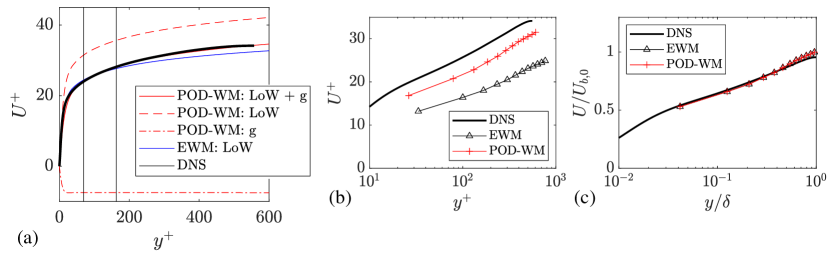
Figure 12: (a) DNS profiles and a-priori WM reconstructions at $tu_{\tau,0}/\delta=0.035$ for case R1000A100. The two vertical lines are at $1.5/12\delta$ and $3.5/12\delta$, which correspond to the 2nd and 4th grid points in our WMLES. The LoW mode and the $g$ mode in the POD-augmented WM are also plotted. This corresponds to $c_{1x}$LoW and $c_{2x}g$. Their contributions to the wall-shear stress are of opposite signs, which is consistent with figure 10. (b, c) Mean velocity profiles from DNS, WMLES with EWM and POD-augmented WM, (b) normalization by inner units, (c) normalization by outer units.

	Reconstruction				WMLES
	$\tau_{w}$: LoW	$\tau_{w}$: g	$\tau_{w}$	error	$\tau_{w}$	error
EWM	0.50	0	0.50	61%	0.67	116%
POD-augmented WM	0.62	-0.24	0.38	23%	0.40	29%

Table 3: Contributions of each mode to the wall-shear stress at time $tu_{\tau,0}/\delta=0.035$ in case R1000A100. The EWM does not contain a $g$ mode, and therefore its contribution to EWM’s prediction is 0. The reconstruction result corresponds to figure 12, and the WMLES result corresponds to figure 11. The wall-shear stress values are normalized with $\rho u^{2}_{\tau,0}$. The DNS value is 0.31, which we take as the truth.

Before we conclude this section, we comment on the presentation of the results. Figure 12(b, c) show the DNS and WMLES profiles at $tu_{\tau,0}/\delta=0.035$ in case R1000A100. At this time instant, the DNS predicts $\tau_{w}=0.31\tau_{w,0}$. The POD-augmented WM predicts $\tau_{w}=0.40\tau_{w,0}$, and the EWM predicts $\tau_{w}=0.67\tau_{w,0}$, leading to a 116% error in EWM’s prediction and a 29% error in POD-augmented WM’s prediction. The EWM is not at all accurate. This, however, is only clear in figure 12(b), where normalization is by the inner units, not in (c), where normalization is by the outer units. Again, this is because the imposed adverse pressure gradient overwhelms the wall-shear stress, and the evolution of the velocity profile is dominated by the imposed pressure gradient for the initial period. We would also like to comment on the flow statistics we show. WMLES and LES, in general, resolve only part of the energy spectrum, and therefore they are not meant to capture turbulence quantities like the velocity rms and the energy spectrum, which is why we have chosen to focus on mean flow quantities.

4.4 Transverse pressure gradient

Last, we apply the POD-augmented WM in a channel subjected to a suddenly imposed TPG. A schematic of the flow was shown in figure 2(b) already. The channel is initially at a Reynolds number $Re_{\tau}=1000$. The magnitude of the TPG is $10(\tau_{w,0}/\delta)$. Table 4 shows the WMLES details. Figure 13(a, b) shows the WMLES result. We observe the following. Firstly, the POD-augmented wall model captures the initial decrease in the streamwise wall-shear stress and gives wall-shear stress predictions that agree more closely with the DNS than the other models (comparing figure 13(a) and figure 2(d)). Secondly, the streamwise wall-shear stress behaves differently from one realization to another, whereas the spanwise wall-shear stress behaves similarly between the different realizations. Thirdly, the POD-augmented WM gives more accurate spanwise wall-shear stress predictions than the EWM.

Repeating the exercise in §4.3, we can show that wall modeling is not critical to the prediction of the flow rate. We can also reconstruct the velocity profiles and explain why the POD-augmented WM outperforms the EWM. These results, however, are repetitive and therefore are not shown here for brevity.

Case	$Re_{\tau,0}$	Grid	Domain	TPG	WM	N
R1000T10	1000	$96\times 12\times 72$	$8\pi\times 2\times 3\pi$	10	EWM, POD-augmented WM	10

Table 4: WMLES details. The normalization is the same as in Table 2. $N$ is the number of independent realizations.

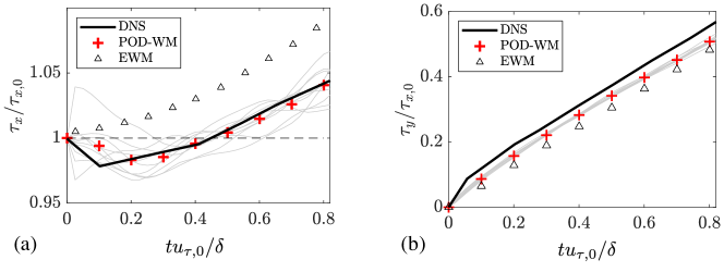
Figure 13: Time evolution of (a) the streamwise wall-shear stress and (b) the spanwise wall-shear stress. The DNS is by Lozano-Durán et al. (2020). The POD-augmented WM results are ensemble averages from 10 statistically independent realizations.

5 Concluding remarks

We augment the LoW by including an additional mode which is based on the first POD mode in a 2D channel for LES wall modeling. The resulting wall model reconstructs the velocity in the wall layer according to

$$\small{\bf U}={\bf c_{1}}{\rm LoW}+{\bf c_{2}}g\,,$$ (14)

where the LoW mode includes the viscous sublayer and the buffer layer, and $g$ is the POD-based mode. The WM and LES match at two off-wall locations instead of one so that one can solve for ${\bf c}_{1}$ and ${\bf c}_{2}$.

The results are promising. The POD-augmented WM captures the rapid decay of the wall-shear stress when a boundary-layer flow is subjected to a large APG. The model also captures the initial decrease in the streamwise wall-shear stress when a boundary-layer flow is subjected to a TPG. Both phenomena had not been captured in WMLES. A-priori analysis shows that the POD-augmented WM captures these phenomena because its ansatz is a more realistic approximation of the mean flow when there is a non-equilibrium pressure gradient. Still, additional testing of the model in other flows will be needed to fully assess its performance. This should include spatially developing flow, flows in complex geometries, and flows with multiple non-equilibrium effects.

This work is the first attempt to apply results from modal analysis for predictive wall modeling in LES, and there is still a lot we can explore. Future work will explore WMs with more modes, modes from other modal analysis techniques (in Appendix B, we explored some other modes), and applications of the model in flows with complex geometries.

Conflict of interest

The authors claim no conflict of interest.

Appendix A Numerical implementation of POD

As we use a one-dimensional scalar variant of POD in this work the numerical implementation is surprisingly simple. We start by collecting realizations of the fluctuating streamwise velocity component along the wall-normal direction $u^{\prime}(y)$. Here $u^{\prime}(y)=u(y)-{\rm LoW}$, such that we have removed the LoW (mean). The realizations are collected from the DNS of a 2D turbulent channel at $Re_{\tau}=5200$ (Lee & Moser, 2015; Graham et al., 2016). We sample the realizations along the wall-parallel directions and at different times as in Moin & Moser (1989). Denoting these discrete realizations as ${\bf u}_{j}$, we follow Holmes et al. (2012) and arrange these into a data matrix

$${\bf X}=\begin{bmatrix}{\bf u}_{1}&\cdots&{\bf u}_{N}\end{bmatrix}\,,$$ (15)

after which the POD analysis can be accomplished by the singular value decomposition

$${\bf X}={\bf U}{\boldsymbol{\Sigma}}{\bf V}^{T}\,.$$ (16)

The columns of U are then the POD modes, while the diagonal matrix ${\boldsymbol{\Sigma}}$ contains the singular values (related to the POD eigenvalues), and ${\bf V}$ carries the POD mode coefficients. For the present work, however, we are only interested in the first POD mode which is contained in the first column of ${\bf U}$.

Appendix B The choice of the g mode

We investigate the sensitivity of the presented results to the choice of the $g$ mode. Specifically, we consider two other choices

$$g_{\rm lin}(y^{+})=y^{+}\,,\qquad g_{\rm rms}(y^{+})\propto u_{\rm rms}(y^{+})\,,$$ (17)

where $u_{\rm rms}$ is the rms of the streamwise velocity fluctuation in a $Re_{\tau}=5200$ plane channel (Lee & Moser, 2015). We normalized $g_{\rm rms}$ such that $\left.dg_{\rm rms}/dy^{+}\right|_{y=0}=1$. This normalization is automatically satisfied for $g_{\rm lin}$. Additionally, we have included an exponential term in $g_{\rm rms}$ to ensure that the mode approaches zero sufficiently far away from the wall. This exponential term has little/no impact on the results shown below as the matching locations used here are within $y^{+}<1000$. The three $g$ modes are shown in figure 14.

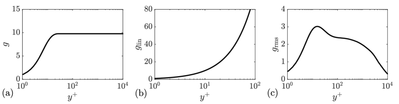
Figure 14: (a) The proposed POD-based $g$ mode. (b) The linear $g$ mode. (c) The rms-based $g$ mode. Note the different scales on both the abscissa and ordinate for better visualization of the three modes.

We first repeat the a-priori tests from §3.2 for cases R1000A10 and R1000A100. The results are shown in figure 15. For case R1000A10, the EWM, LIN-WM, and POD-WM yield similar predictions; the RMS-WM, on the other hand, predicts a low wall-shear stress within the range $0\leq tu_{\tau,0}/\delta\leq 0.5$. For case R1000A100, the four models all give different wall-shear stress predictions. The LIN-WM demonstrates only a slight improvement over the EWM, with both models overestimating the wall-shear stress. In contrast, the POD-WM exhibits substantial improvement compared to the EWM and LIN-WM. Meanwhile, the RMS-WM underestimates the wall-shear stress.

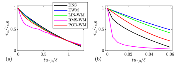
Figure 15: A-priori results for cases R1000A10 and R1000A100. (a) Wall-shear stress from DNS, the EWM, the LIN-WM, the RMS-WM, and the POD-WM in case R1000A10. (b) Same as (a) but for case R1000A100.

Next, we investigate how the a-posteriori results for the R1000A10 and R1000A100 cases, discussed in §4.3, are affected when employing different $g$ modes specified in (17). These results are presented in figure 16. Figure 16(a) shows that the EWM, LIN-WM, RMS-WM, and POD-WM all perform well for the R1000A10 case, with their wall-shear stress predictions closely matching the DNS results. For the R1000A100 case shown in 16(b), we observe that the EWM and LIN-WM over-predict the wall-shear stress with the LIN-WM being slightly more accurate. The RMS-WM under-predicts the wall-shear stress by a considerable amount. Furthermore, the simulation blows up at around $tu_{\tau,0}/\delta\approx 0.02$, when violent fluctuations in the local wall-shear stresses are found. Among the four models, the POD-WM results are the closest to the DNS data.

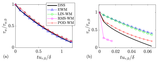
Figure 16: A-posteriori results for cases R1000A10 and R1000A100. (a) Wall-shear stress from DNS, the EWM, the LIN-WM, the RMS-WM, and the POD-WM for case R1000A10. (b) Same as (a) but for case R1000A100. The RMS-WM result is cut off at $tu_{\tau,0}/\delta\approx 0.02$ because the WMLES simulation blows up at this point.

Finally, the TPG a-posteriori results from §4.4, i.e., the R1000T10 case, are revisited. The results from the EWM, LIN-WM, RMS-WM, and POD-WM are shown in figure 17. For the streamwise wall-shear stress, shown in figure 17(a), we see that the LIN-WM does not convincingly capture the initial decrease and slightly over-predicts the wall-shear stress during its increase. The RMS-WM, on the other hand, captures the initial decrease in the streamwise wall-shear stress but under-predicts wall-shear stress for the remaining part. Turning to the spanwise wall-shear stress in figure 17(b), we observe that there is much less variability in the results. The EWM, LIN-WM, and POD-WM perform similarly, with both the LIN-WM and POD-WM showing minor improvements compared to the EWM. The RMS-WM exhibits the closest agreement with the DNS data in the initial period.

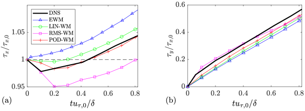
Figure 17: A-posteriori results for case R1000T10. (a) Streamwise wall-shear stress from DNS, the EWM, the LIN-WM, the RMS-WM, and the POD-WM in case R1000T10. (b) Same as (a) but for spanwise wall-shear stress.

In all, we see that the choice of the $g$ mode does make a difference to the results.

References

- Abkar & Moin (2017) Abkar, M. & Moin, P. 2017 Large-eddy simulation of thermally stratified atmospheric boundary-layer flow using a minimum dissipation model. Boundary-Layer Meteorol. 165, 405–419.
- Aubry et al. (1988) Aubry, N., Holmes, P., Lumley, J. L. & Stone, E. 1988 The dynamics of coherent structures in the wall region of a turbulent boundary layer. J. Fluid Mech. 192, 115–173.
- Bae et al. (2019) Bae, H. J., Lozano-Durán, A., Bose, S. T. & Moin, P. 2019 Dynamic slip wall model for large-eddy simulation. J. Fluid Mech. 859, 400–432.
- Berkooz et al. (1993) Berkooz, G., Holmes, P. & Lumley, J. L. 1993 The proper orthogonal decomposition in the analysis of turbulent flows. Annual review of fluid mechanics 25 (1), 539–575.
- Bose & Moin (2014) Bose, S. & Moin, P. 2014 A dynamic slip boundary condition for wall-modeled large-eddy simulation. Phys. Fluids 26, 015104.
- Bose & Park (2018) Bose, S. T. & Park, G. I. 2018 Wall-modeled large-eddy simulation for complex turbulent flows. Ann. Rev. Fluid Mech. 50, 535–561.
- Bou-Zeid et al. (2005) Bou-Zeid, E., Meneveau, C. & Parlange, M. 2005 A scale-dependent lagrangian dynamic model for large eddy simulation of complex turbulent flows. Phys. Fluids 17, 025105.
- Chen et al. (2022) Chen, P. E., Lv, Y., Xu, H. H., Shi, Y. & Yang, X. I. A. 2022 LES wall modeling for heat transfer at high speeds. Phys. Rev. Fluids 7 (1), 014608.
- Choi & Moin (2012) Choi, H. & Moin, P. 2012 Grid-point requirements for large eddy simulation: Chapman’s estimates revisited. Phys. Fluids 24, 011702.
- De Vanna et al. (2021) De Vanna, F., Cogo, M., Bernardini, M., Picano, F. & Benini, E. 2021 Unified wall-resolved and wall-modeled method for large-eddy simulations of compressible wall-bounded flows. Phys. Rev. Fluids 6, 034614.
- Fowler et al. (2022) Fowler, M., Zaki, T. A. & Meneveau, C. 2022 A Lagrangian relaxation towards equilibrium wall model for large eddy simulation. J. Fluid Mech. 934, A44.
- Goc et al. (2021) Goc, K. A., Lehmkuhl, O., Park, G. I., Bose, S. T. & Moin, P. 2021 Large eddy simulation of aircraft at affordable cost: a milestone in computational fluid dynamics. Flow 1, E14.
- Graham et al. (2016) Graham, J., Kanov, K., Yang, X. I. A., Lee, M., Malaya, N., Lalescu, C., Burns, R., Eyink, G., Szalay, A., Moser, R. & others 2016 A web services accessible database of turbulent channel flow and its use for testing a new integral wall model for LES. J. Turbul. 17, 181–215.
- He & Seddighi (2015) He, S. & Seddighi, M. 2015 Transition of transient channel flow after a change in Reynolds number. J. Fluid Mech. 764, 395–427.
- Holmes et al. (2012) Holmes, P., Lumley, J. L., Berkooz, G. & Rowley, C. W. 2012 Turbulence, coherent structures, dynamical systems and symmetry. Cambridge university press.
- Kawai & Larsson (2012) Kawai, S. & Larsson, J. 2012 Wall-modeling in large eddy simulation: Length scales, grid resolution, and accuracy. Phys. Fluids 24, 015105.
- Kim et al. (1987) Kim, J., Moin, P. & Moser, R. 1987 Turbulence statistics in fully developed channel flow at low Reynolds number. J. Fluid Mech. 177, 133–166.
- Larsson et al. (2016) Larsson, J., Kawai, S., Bodart, J. & Bermejo-Moreno, I. 2016 Large eddy simulation with modeled wall-stress: recent progress and future directions. Mech. Eng. Rev. 3, 15–00418.
- Lee & Moser (2015) Lee, M. & Moser, R. D. 2015 Direct numerical simulation of turbulent channel flow up to Re. J. Fluid Mech. 774, 395–415.
- Lozano-Durán et al. (2020) Lozano-Durán, A., Giometto, M. G., Park, G. I. & Moin, P. 2020 Non-equilibrium three-dimensional boundary layers at moderate Reynolds numbers. J. Fluid Mech. 883, A20.
- Lozano-Durán & Jiménez (2014) Lozano-Durán, A. & Jiménez, J. 2014 Effect of the computational domain on direct simulations of turbulent channels up to Reτ= 4200. Phys. Fluids 26, 011702.
- Lv et al. (2021) Lv, Y., Huang, X. L. D., Yang, X. & Yang, X. I. A. 2021 Wall-model integrated computational framework for large-eddy simulations of wall-bounded flows. Phys. Fluids 33, 125120.
- Moin & Moser (1989) Moin, P. & Moser, R. D. 1989 Characteristic-eddy decomposition of turbulence in a channel. J. Fluid Mech. 200, 471–509.
- Monty et al. (2011) Monty, J. P., Harun, Z. & Marusic, I. 2011 A parametric study of adverse pressure gradient turbulent boundary layers. Int J Heat Fluid Flow 32, 575–585.
- Na & Moin (1998) Na, Y. & Moin, P. 1998 Direct numerical simulation of a separated turbulent boundary layer. J. Fluid Mech. 374, 379–405.
- Park & Moin (2014) Park, G. I. & Moin, P. 2014 An improved dynamic non-equilibrium wall-model for large eddy simulation. Phys. Fluids 26, 015108.
- Park & Moin (2016) Park, G. I. & Moin, P. 2016 Numerical aspects and implementation of a two-layer zonal wall model for LES of compressible turbulent flows on unstructured meshes. J Comput Phys 305, 589–603.
- Piomelli & Balaras (2002) Piomelli, U. & Balaras, E. 2002 Wall-layer models for large-eddy simulations. Ann. Rev. Fluid Mech. 34, 349–374.
- Reichardt (1951) Reichardt, H. 1951 Vollständige darstellung der turbulenten geschwindigkeitsverteilung in glatten leitungen. ZAMM-Journal of Applied Mathematics and Mechanics/Zeitschrift für Angewandte Mathematik und Mechanik 31 (7), 208–219.
- Schumann (1975) Schumann, U. 1975 Subgrid scale model for finite difference simulations of turbulent flows in plane channels and annuli. J. Comput. Phys. 18 (4), 376–404.
- Spalding (1961) Spalding, D. B. 1961 A single formula for the law of the wall. Journal of Applied mechanics 28 (3), 455–458.
- Taira et al. (2017) Taira, K., Brunton, S. L., Dawson, S. T., Rowley, C. W., Colonius, T., McKeon, B. J., Schmidt, O. T., Gordeyev, S., Theofilis, V. & Ukeiley, L. S. 2017 Modal analysis of fluid flows: An overview. AIAA Journal 55 (12), 4013–4041.
- Volino (2020) Volino, R. J. 2020 Non-equilibrium development in turbulent boundary layers with changing pressure gradients. J. Fluid Mech. 897, A2.
- Yang & Abkar (2018) Yang, X. I. A. & Abkar, M. 2018 A hierarchical random additive model for passive scalars in wall-bounded flows at high Reynolds numbers. J. Fluid Mech. 842, 354–380.
- Yang et al. (2022) Yang, X. I. A., Chen, P. E., Hu, R. & Abkar, M. 2022 Logarithmic-linear law of the streamwise velocity variance in stably stratified boundary layers. Boundary-Layer Meteorol. 183, 199–213.
- Yang & Griffin (2021) Yang, X. I. A. & Griffin, K. P. 2021 Grid-point and time-step requirements for direct numerical simulation and large-eddy simulation. Phys. Fluids 33, 015108.
- Yang & Lv (2018) Yang, X. I. A. & Lv, Y. 2018 A semi-locally scaled eddy viscosity formulation for LES wall models and flows at high speeds. Theor Comp Fluid Dyn 32 (5), 617–627.
- Yang et al. (2017) Yang, X. I. A., Park, G. I. & Moin, P. 2017 Log-layer mismatch and modeling of the fluctuating wall stress in wall-modeled large-eddy simulations. Phys. Rev. Fluids 2, 104601.
- Yang et al. (2015) Yang, X. I. A., Sadique, J., Mittal, R. & Meneveau, C. 2015 Integral wall model for large eddy simulations of wall-bounded turbulent flows. Phys. Fluids 27, 025112.
- Yang et al. (2019) Yang, X. I. A., Zafar, S., Wang, J.-X. & Xiao, H. 2019 Predictive large-eddy-simulation wall modeling via physics-informed neural networks. Phys. Rev. Fluids 4 (3), 034602.