Learning from Very Little Data: On the Value of Landscape Analysis for Predicting Software Project Health

Abstract.

When data is scarce, software analytics can make many mistakes. For example, consider learning predictors for open source project health (e.g. the number of closed pull requests in twelve months time). The training data for this task may be very small (e.g. five years of data, collected every month means just 60 rows of training data). The models generated from such tiny data sets can make many prediction errors.

Those errors can be tamed by a landscape analysis that selects better learner control parameters. Our niSNEAK tool (a) clusters the data to find the general landscape of the hyperparameters; then (b) explores a few representatives from each part of that landscape. niSNEAK is both faster and more effective than prior state-of-the-art hyperparameter optimization algorithms (e.g. FLASH, HYPEROPT, OPTUNA).

The configurations found by niSNEAK have far less error than other methods. For example, for project health indicators such as $C$= number of commits; $I$=number of closed issues, and $R$=number of closed pull requests, niSNEAK’s 12 month prediction errors are {I=0%, R=33% C=47%} while other methods have far larger errors of {I=61%,R=119% C=149%}. We conjecture that niSNEAK works so well since it finds the most informative regions of the hyperparameters, then jumps to those regions. Other methods (that do not reflect over the landscape) can waste time exploring less informative options.

Based on the above, we recommend landscape analytics (e.g. niSNEAK) especially when learning from very small data sets. This paper only explores the application of niSNEAK to project health. That said, we see nothing in principle that prevents the application of this technique to a wider range of problems.

To assist other researchers in repeating, improving, or even refuting our results, all our scripts and data are available on GitHub at https://github.com/zxcv123456qwe/niSneak.

1. Introduction

Open source software (OSS) projects are most successful when they are supported by a large community of developers. Such support can take many important forms including (a) programmer time (to fix bugs or write documentation or build APIs); (b) financial donations (to fund infrastructure); or (c) public endorsements (e.g. when companies join the board of directors of OSS foundations).

Attracting such support is easier when projects show healthy trends in their development. Many researchers comment that healthy OSS projects are characterized by much developer activity (Wahyudin et al., 2007; Jansen, 2014; Manikas and Hansen, 2013; Link and Germonprez, 2018; Wynn Jr, 2007; Crowston and Howison, 2006). For example, Han et al. note that popular open-source software (OSS) projects tend to be more active (Han et al., 2019). Accordingly, we seek to improve methods that predict the future activity of an OSS project (e.g. number of closed pull requests in twelve months time).

Sarro et al. (Sarro et al., 2016) assert that for this kind of project estimation, acceptable error rates are 30% to 40% (measured as abs(actual - predicted)/ actual). But when project data is limited, it is hard to meet Sarro’s requirements. For example, consider the task of learning an OSS health predictor using the 60 rows (ish) of data that can be extracted from such projects. As we will show below, the models learned from such small data sets have error rates much worse than the limits stated by Sarro et al.

We show here that a new optimizer called niSNEAK, based on landscape analytics, can dramatically reduce prediction errors, even when learning models from very little data. Landscape analytics (Malan, 2021; Bosman et al., 2020; Mersmann et al., 2011; Ochoa et al., 2008; Belaidouni and Hao, 1999) maps out the space of data being explored in order to find the most information-rich part of the data. Once that is known, then we can leap to the more informative parts of the problem space. Most landscape analytics methods require a pre-enumeration of most of the space (Malan, 2021). But in the case of predicting for open source project health, this is impractical. For example, Table 1 lists 960,000 different ways a learner might be configured for predicting open source project health. Assuming five seconds per learner (which might be an underestimate), then a study of all 960,000 options, repeated 20 times (to check for external validity) would terminate after $960,000*5/(3600*24)*20=1,111$ days (and note that if Table 1 explored more options or more learners, or slower methods such as deep learning, then those runtimes would get even longer.)

Parameter	Min	Max	Step	#options
n_estimators	10	200	10	20
min_sample_leaves	1	20	1	20
min_impurity_decrease	0	10	0.25	40
max_depth	1	20	1	20
criterion	one of: [squared, absolute, poisson]			3
			Total (20*20*40*20*3):	960,000

Table 1. Options for ensembles of regression trees.

Landscape analytics can reduce the cost of that search. For example, niSNEAK can find configurations that result in low errors after looking at around 100 options (while other tools needed to examine thousands more options (Akiba et al., 2019; Bergstra et al., 2011)). Not only that, but niSNEAK’s predictions have errors rates within the Sarro et al. limits. In fact, when predicting for one particular project health indicator (number of closed issues), we found a median error rate of 0%. We conjecture that those other optimizers performed worse since they used a somewhat uninformed search based on random mutations. On the other hand, niSNEAK works well because it carefully reflects on the shape of the data before deciding where to go next.

This paper explores three research questions:

• RQ1 - Does small sample size damage our ability to perform project health prediction?. This is our baseline question. The central motivation of this paper is that small sample sizes in analytics can lead to errors in project health estimation. Hence, before this paper does anything else, we need to back up that claim. What we will show as part of RQ1 is that many methods in common use perform very badly on our tiny data sets.

• RQ2 - Can landscape analysis mitigate for small sample sizes? Here, we compare the better results from RQ1 (that make no use of landscape analysis) with the new methods of this paper (that use landscape analysis). As shown in the RQ2 results, adding landscape analysis significantly improves our ability to make predictions about very small data sets.

• RQ3 - How much landscape analysis is enough? This question is somewhat technical and addresses some internal design decisions. niSNEAK runs in multiple sweeps across the landscape where each sweep focuses on a different part of the data (e.g. one sweep only looks at the dependent variables while another only looks at the independent values). This raises the question of whether we are “sweeping” too much or too little. As seen by the results of RQ3, some sweeping is better than no sweeping, and too much is contraindicated.

The rest of this paper is structured via guidelines from Wohlin & Runeson et al. (Wohlin et al., 2012) on empirical software engineering. We present our methods in §3, define and explain our case study and in §4, then show results in §5. See also §6 for a discussion on the threats to the validity of our conclusions.

2. Background

2.1. Motivation

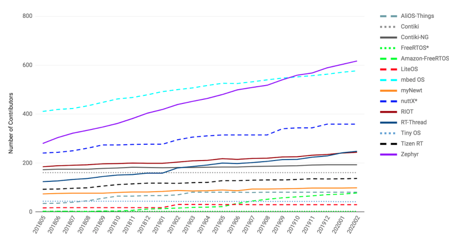
Figure 1. Trends in number of contributors across 14 real-time OS projects since 2018. Zephyr (purple) has out-paced other similar software projects.

Feature	Description
dates	The end date of monthly data collection
monthly commits	Total number of commits created in last month
monthly commit comments	Total number of commit comments created in last month
monthly contributors	Total number of contributors that at least have one commit in last month
monthly open PRs	Total number of pull requests opened in last month
monthly closed PRs	Total number of pull requests closed in last month
monthly merged PRs	Total number of pull requests merged in last month
monthly PR mergers	Total number of pull requests mergers in last month
monthly PR comments	Total number of pull request comments created in last month
monthly open issues	Total number of issues opened in last month
monthly closed issues	Total number of issues closed in last month
monthly issue comments	Total number of issue comments created in last month
monthly stargazer	Total number of new stars acquired in last month
monthly forks	Total number of forks occurred in last month
monthly watchers	Total number of new watchers acquired in last month

Table 2. Project health indicators. From Xia et al.  (Xia et al., 2022b).

This section explains our motivation for exploring open source project health.

In summary, in many scenarios, it is important to predict future health (or, if that health is declining, to take steps to address that issue). For example, many commercial companies use open-source packages in the products they sell to customers. Those companies seek projects that they trust will remain viable for the foreseeable future.

Also, projects with an unhealthy reputation lose their community support. This is not ideal since OSS projects grow when they attract developers. Large OSS projects (e.g. the LINUX or APACHE foundation) have board members representing organizations that allocate considerable resources to maintaining and extending software. Attracting such investments is far easier when projects can show potential investors healthy trends in their project development. For example, in the Apache ecosystem, there are 14 real-time time operating systems. Measured in terms of code commits per month, Figure 1 shows that most of these are stagnant (e.g. LiteOS and myNewt), while the remaining two (Zephyr and mbed OS) show a strong increase in the number of commits per month.

There are many ways to document those trends and, for our research, we use a list of trend indicators selected by a survey by hundreds of decision-makers from dozens of open source projects (Xia et al., 2022a). In that survey, it was found that decision-makers wanted methods to predict open source health indicators of Table 2 such as commits; closed pull requests; and number of contributors.

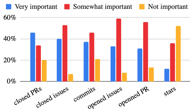
Figure 2. Importance of indicators to OSS developers. PR=pull requests. From (Xia et al., 2022b).

Figure 2 shows the results when Xia et al. (Xia et al., 2022b) asked developers to rank the indicators. That survey sought the opinion of “core developers”; i.e. those who make pivotal decisions about software. Xia et al. found 112 core contributors from 68 projects and asked them “what product health indicators would prompt them to take action within their project?”. Some indicators were not so important (e.g. number of stars assigned to a project in GitHub) while others were seen to be far more valuable (e.g. closed pull requests).

The rest of this paper explores methods for predicting the items in Figure 2 that were ranked largest in terms of “very important” (a) number of closed issues, and (b) number of closed pull requests; and (c) number of commits.

2.2. Differences to Related Work

Before going further, we digress here to distinguish this work from prior research.

Traditionally, in the age of waterfall projects, project effort predictions tried to guess the funds required for project completion. To do so, some nominal estimate was generated (which was then inflated according to known risk factors inside a project). For example, Boehm et al.’s COCOMO model (Chulani et al., 1999) (developed in 1981 and updated in 2000) generated estimates of total project effort (measured in terms of 150-hour work-months) that were within 30% of actual, 71% of the time. Robbles et al. (Robles et al., 2022) report that for a large class of OSS projects, developers will spend much of their time working full time on a single project. Hence, for those projects, it is possible to estimate the total effort that will be spent on a project, early in its development using (as shown by Robbles et al.) project features extracted from an online version control systems (e.g. GitHub).

Robbles’ work inspired Xia et al (Xia et al., 2022b) to try applying the Boehm methods to OSS teams; specifically the APACHE and LINUX kernel development teams. Xia et al. found that those teams expressed little interest in estimates of “effort to finish”, since no one in these teams expected to ever “finish” their projects (those developers are funded in perpetuity to maintain and extend their tools).

Since Xia et al. had so much trouble with waterfall-style estimation, in this work we explore health indicators that can be applied to on-going projects. Many researchers have explored such health indicatiors (Bao et al., 2019; Jarczyk et al., 2018; Kikas et al., 2016; Han et al., 2019; Qi et al., 2017; Chen et al., 2014; Wahyudin et al., 2007; Jansen, 2014; Manikas and Hansen, 2013; Link and Germonprez, 2018; Wynn Jr, 2007; Crowston and Howison, 2006). For example, Bao et al. (Bao et al., 2019) apply Naive Bayes, SVR, Decision Tree, KNN and Random Forest to 917 projects from GHTorrent to predict long term contributors (which they determine as the time interval between their first and last commit in the project is larger than a threshold.). They found random forest achieves the best performance. Kikas et al. (Kikas et al., 2016) built random forest models to predict the issue close time on GitHub projects, with multiple static, dynamic and contextual features. They report that the dynamic and contextual features are critical in such prediction tasks. Jarczyk et al. (Jarczyk et al., 2018) used generalized linear models for predictions of issue closure rate. Based on multiple features (stars, commits, issues closed by the team, etc.), they found that larger teams with more project members have lower issue closure rates than smaller teams, while increased work centralization improved issue closure rates. Other developing related feature predictions also include the information on commits, which is used by Qi et al. (Qi et al., 2017) in their software effort estimation research of OSS projects, where they treat the number of commits as an indicator of human effort. Chen et al. (Chen et al., 2014) used linear regression models on 1,000 GitHub projects to predict the number of forks; they concluded that this prediction could help GitHub recommend popular projects and guide developers to find projects that are likely to succeed and worthy of their contribution.

There are several important differences between our work and the above. For the most part, the above explored a single measure of project health (and not the many measures explored here). Also, their data collection methods were somewhat opportunistic in that they seem to have found a data source, then taken steps to exploit that data. We say this since when we went looking for their kinds of data, we often found that the available information was somewhat different to that used in the above. Like Xia et al., we found that, for many projects, we could reliably collect information about the Table 2 items. Hence, we base our predictors on those attributes.

Another difference of our work to the above is that, with the exception of Bao et al. (Bao et al., 2019), most of the prior work used data miners without hyperparameter optimization. The importance of hyperparameter optimization is discussed in the next section.

2.3. Hyperparameter Optimization

When a learner executes, it uses many decisions about what things to explore and what things to ignore. Those decisions are controlled by the hyperparameters of the learner. Example hyperparameters include (a) how many neighbors to use in nearest neighbor classification or (b) how many trees to include in a random forest or (c) how to configure the architecture of a deep learner.

Hyperparameter optimization is a very active field of research. A common result in software analytics (Agrawal and Menzies, 2018; Agrawal et al., 2019, 2020; Fu et al., 2016a, b; Xia et al., 2020; Tu and Menzies, 2021, 2022a; Yu et al., 2022) (and other domains outside of SE (Bergstra et al., 2011; Storn and Price, 1997; Nair et al., 2018; Chen et al., 2018; Akiba et al., 2019; Tu et al., 2021)) is that automatic hyperparameter optimization can find settings that dramatically improve some algorithm. We list below some of the algorithms commonly seen in the literature. Our reading of the literature is that, of the following, HYPEROPT and OPTUNA represent the prior state-of-the-art. One complaint we have against the Xia et al. analysis is that they made scant use of those state-of-the-art tools (their paper makes only one small study with HYPEROPT, on limited data).

2.3.1. Grid Search (GS) (Bergstra et al., 2011)

As described by Bergstra et al. (Bergstra et al., 2011), GS defines all hyperparameter options in a set of vectors. GS then executes over the cross product of those options. Note that GS will execute all combinations, and as such for limiting CPU usage one must define a smaller search.

2.3.2. Random Search (RS) (Bergstra et al., 2011)

Random search starts with the same option vectors as grid search. But instead of evaluating all of the models in the grid, RS evaluates a random subset of these models selecting the best configuration from this subset. Both GS and RS have been previously used towards the optimization of models for defect prediction (Nevendra and Singh, 2022).

2.3.3. Differential Evolution (DE) (Storn and Price, 1997)

Differential Evolution is an evolutionary algorithm that executes in several generations of mutate-crossover-select. DE starts like random search and creates a small initial population of randomly selected configuration options (say, 10 vectors of options per feature being configured). For each generation, each option is compared to a newly created option that is a mixture of three other options in the population. The new option replaces the old, if it is better. After generation#1, the invariant of DE is that each option in a population in generation $g$ is superior to at least $g-1$ other options. Hence, as the generations mature, DE mixes together new items built from items of increasing superior options. DE was previously used for defect prediction by (e.g.) Fu et al. (Fu et al., 2016a) on data from open-source JAVA systems.

2.3.4. FLASH (Nair et al., 2018)

FLASH is a sequential model-based optimization (SMBO) method, introduced by Nair et al. (Nair et al., 2018), that outperformed the then-known state-of-the-art. SMBO methods use a surrogate model built from options-evaluated-to-date to make guesses about all the as-yet unevaluated options. Then (a) the “most interesting” option is then evaluated, and (b) the surrogate is then updated so that we can make better guesses in the future. When used in practice, FLASH’s surrogate model might make 100,000s of very fast guesses in order to select the best $10^{1}$ to $10^{2}$ configurations that actually deserve evaluation. Nair et al. used FLASH to find the best possible configurations for 7 different software systems.

2.3.5. SWAY (Chen et al., 2018)

The SWAY oversampling approach recursively clusters 10,000 randomly generated configurations (perhaps generated via theorem prover from domain constraints). SWAY is a greedy-search algorithm that always commits to the topmost partition (without checking if any other partition is better). Later in this paper, we will discuss (§3.1.2) the Zitzler domination predicate and other details present in SWAY. Previously, in software engineering, SWAY (Chen et al., 2018) was applied towards the optimization of software process models and software product lines.

2.3.6. HYPEROPT (Bergstra et al., 2015)

HYPEROPT is a hyperparameter optimization framework introduced in 2015 as a Python package. At the time of this writing, the two papers that lead to HYPEROPT (Bergstra and Bengio, 2012; Bergstra et al., 2011) have been cited 7668 and 3543 times, making this the most mentioned algorithm in this survey. At its core, it uses either RS or the Tree-Parzen Estimator (TPE) as the optimization algorithm. TPE is an SMBO algorithm introduced by Bergstra et al. (Bergstra et al., 2011), that will model the sequential model optimization via the use of non-parametric statistical densities. Yedida et al. (Agrawal et al., 2021; Yedida and Menzies, 2021) have used HYPEROPT for software defect prediction. Classic HYPEROPT does not allow for multi-objective optimization so when we use it, we will just tune to minimize the magnitude of relative error (MRE) values.

2.3.7. OPTUNA (Akiba et al., 2019)

OPTUNA is a more recent hyperparameter optimization framework than HYPEROPT that uses MOTPE (Ozaki et al., 2020), a more advanced version of TPE. MOTPE allows for the optimization of multiple performance metrics at once by analyzing the results of the current models against the currently observed frontier of solutions via using a function that calculates the expected hypervolume improvement at each step of its optimization. To the best of our knowledge, OPTUNA has not been used extensively for software engineering problems (but it has been used in domains such as disease diagnosis (Zhou et al., 2022), equipment performance forecast (Mashlakov et al., 2019) and others). We assert that it is important to baseline our new methods against OPTUNA (and MOTPE) since this is a clear extension and improvement of HYPEROPT.

2.4. Landscape Analytics

The experiments of this paper show that, at least for predicting future trends in OSS projects, we can outperform all of the above hyperparameter optimization methods through landscape analytics. This section describes that kind of analytics.

To understand landscape analytics, consider a function:

(1) $$Y=f(X)$$

where $X$ contains one or more independent features and $Y$ contains one or more dependent features. If we cluster together with the $X$ points or the $Y$ points, we can draw out the shape of the data. We call this shape the “landscape”.

The process of data mining can be characterized as a search across landscapes. Given many examples of $(X_{1},Y_{1}),(X_{2},Y_{2}),..\mathit{etc}$ then a learner $L$ seeks some model $f$ that knows where parts of the $X$ landscape connect to particular parts of the $Y$ landscape. Also, a learner may contain hyperparameters $W$ about (e.g.) how many neighbors to use in the nearest neighbor classifier or (e.g.) how many times to divide numerics. Different hyperparameters will result in different models, so we must rewrite Equation 1 as:

(2) $$Y=L(W)(X)$$

To further guide that search of the hyperparameters, we note that in most domains, there is some preference function $P$ that tells us which parts of the dependent landscape are better than others. E.g. if $Y$ contains some measure of false alarms, then lower false alarms might be scored higher. Within this framework, the goal of hyperparameter optimization is to find the hyperparameters $W$ that lead to dependent variable settings that maximize the score:

(3) $$\mathop{\mathrm{argmax}}_{w_{i}\subseteq W}\left(P(L(w_{i})(X))\right)$$

The list of all $W$ configurations also forms a landscape (separate to the $X,Y$ landscapes). Landscape Analytics is the process of understanding and then exploiting the shape of these landscapes. Not all landscapes are “cliffs” where the data changes suddenly and steeply. When changing many options has similar effects, the landscape can be quite smooth and easily mapped out with just a few samples. Hence, many methods (Liu et al., 2016; Van Engelen and Hoos, 2020; Ros et al., 2017; Chapelle et al., 2006; Tu and Menzies, 2022b) reason by cluster the data, then explore just a few representatives from each cluster. To say that another way, when the landscape is smooth, it is not necessary to search everywhere. Rather, it can be (much) faster to:

1. Look around that space with just a few samples;

2. Then leap over to regions of denser information.

While it is not widely acknowledged, in our opinion, landscape analytics generalizes a range of algorithms from different fields:

Assumption	Notes	# of papers	Example
Binary space	All features have arity=2 and are often used in a theorem prover.	11	HDBL (Belaidouni and Hao, 1999)
Fully enumerable space	The entire search space can be pre-enumerated and cached.	12	LON (Ochoa et al., 2008)
Continuous space	Useful for (e.g.) gradient descent. Discrete features not allowed.	5	ELA (Mersmann et al., 2011)
Knowledge of optima	The value of the achievable best solution already known.	10	Static-$\phi$ (Whitley et al., 1995)
Evalaution is fast/cheap	Optimizers can call the evaluation function 1,000,000s of times.	11	LGC (Bosman et al., 2020)

Table 3. Assumptions made in landscape analytics methods surveyed by Malan (Malan, 2021).

1. When used on the $X$ shape, landscape analytics might be called “clustering”.

2. When used on the $X,Y$ shape, limited sampling might be called “semi-supervised learning”;

3. Similarly, in a joint analysis of the $X,Y$ shape, if we bias our “leaps” towards regions that (in the past) had good $Y$ scores, landscape analytics might be called “reinforcement learning”.

4. And if we use landscape analytics to jointly explore the $W,Y$ shapes, then this could be called “hyperparameter optimization”.

In a recent survey of landscape analytics methods, Malan (Malan, 2021) notes that the term “landscape” is a generalization of Sewell’s 1932 concept of “fitness landscape” (Wright, 1932) which was first defined for evolutionary biology. Malan reports no less than 33 “families” of landscape analytics methods. Most of these methods tend to enumerate the whole landscape, before exploring it. This approach is seen in many parts of the Table 3 summary of the Malan survey; e.g.:

1. Methods that assume that evaluation is fast or cheap usually exploit that property to make many samples across the landscape.

2. Methods that assume knowledge of optima also assume that the search space has been pre-explored (to find that best point).

3. Methods that require a fully enumerable space, by definition, must generate the whole space before reasoning can begin.

For hyperparameter optimization, it is problematic to explore and cache a large part of the search space. This is especially true when conducting large experiments and/or exploring slower data mining algorithms (e.g. deep learners). Quite apart from CPU issues, there are other reasons we need to look beyond standard landscape analytics tools. As shown in Table 3:

• Many current landscape analytics methods require knowledge of optima. For many data mining applications, the achievable maximum is not recall=1, false alarm=0 but some point struggling to achieve (but not reaching) that zenith.

• Many current landscape analytics methods cannot handle features of mixed types since they rely on (e.g.) gradient descent over a continuous space or (e.g.) theorem proving executed on a binary space. This is problematic for hyperparameter optimization since the policies that control data miners are often a combination of numeric and discrete choices.

For these reasons, we built our own landscape analytics tool, differing from existing ones with the following properties:

• It can explore heterogeneous data (discrete and symbolic data) using simple discretization algorithms.

• It only enumerates a subset of the $W,X$ hyperparameters and independent features.

• It only enumerates a small subset of the $Y$ independent features.

That tool is called niSNEAK and is described in the next section.

3. About niSNEAK

niSNEAK is based on Chen et al.’s SWAY algorithm (Chen et al., 2018). It takes a binary dataset comprising of multiple configurations as an input and outputs (a) a binary tree of clustered configurations, from which it reports (b) the best configuration. While an interesting prototype, SWAY suffers from some serious drawbacks. Both SWAY and niSNEAK recursively partition the data, but SWAY’s greedy search always commits to the top-most partition (without checking if any other partition is better), whereas niSNEAK takes a global approach. Specifically, after all the data is clustered, niSNEAK reflects over all the nodes to find which sub-clusters “best” split the data (and “best” means “splits the data such that some attribute range most separates the two splits”).

As such we include SWAY as a baseline algorithm when performing this hyperparameter optimization task.

3.1. Preliminaries

To understand niSNEAK, , we must first what it means to “evaluate” in order to find “better” options.

3.1.1. “Evaluation”

Evaluation means configuring a learner with a set of hyperparameters, running it on some training data, then applying the resulting model to test data.

3.1.2. “Better”

The result of such an evaluation is a set of performance measures associated with a working learner. As shown in Table 4, we have four such measures (Pred40, SA, MRE, D2H). When dealing with multiple goals, a domination predicate is required to decide if one set of performance measures $A=\{\mathit{Pred40}_{i},\mathit{SA}_{i},\mathit{MRE}_{i},\mathit{D2H}_{i}\}$ is “better” than $B=\{\mathit{Pred40}_{j},\mathit{SA}_{j},\mathit{MRE}_{j},\mathit{D2H}_{j}\}$. Two such predicates are boolean domination and the Zitzler multi-objective indicator (Zitzler et al., 2002). Boolean domination says one thing is better than another if it is no worse on any single goal and better on at least one goal. We prefer Zitzler to boolean domination since we have a four-goal optimization problem, and it is known that boolean domination often fails for two or more goals (Wagner et al., 2007; Sayyad et al., 2013). Zitzler favors $B$ over $A$ model if jumping to $A$ “loses” most:

• Let$\textit{worse}(A,B)=\textit{loss}(A,B)>\textit{loss}(B,A)$

• Let $\textit{loss}(A,B)=\sum_{j=1}^{n}-e^{\Delta(j,A,B,n)}/n$

• Let $\Delta(j,A,B,n)=w_{j}(o_{j,A}-o_{j,B})/n$

where “$n$” is the number of objectives (for us, $n=4$) and $w_{j}\in\{-1,1\}$ depending on whether we seek to maximize goal $x_{j}$ and $o_{j,A},o_{j,B}$ are the scores seen for objective $o_{j}$ for $A,B$, respectively.

We assess our project health predictors via widely-used criteria from the literature (Reddy et al., 2010; Sarro et al., 2016; Shepperd and MacDonell, 2012). • MRE is the “magnitude of relative error” and can be computed from abs(actual - predicted)/ actual. • Pred40 assesses the Sarro limit and is defined as $\mathit{Pred40}=\mathit{Count(MREs,}\leq 40)/||\mathit{MREs}||$ • Standardized accuracy (SA) baselines the observed error against some reasonable, fast, but unsophisticated measurement. SA is based on the Mean Absolute Error (MAE) i.e. $\mathit{MAE}=\frac{1}{N}\sum_{i=1}^{n}|\mathit{PREDICT}_{i}-\mathit{ACTUAL}_{i}|$ where $N$ is the size of the test set used for evaluating performance. SA then is defined as the ratio $\mathit{SA}=(1-(\mathit{MAE}/\mathit{MAE}_{\mathit{guess}}))\times 100$ • $\mathit{MAE_{guess}}$ (used in SA) is the $\mathit{MAE}$ of a set of guesses. This paper follows the standards defined by Xia et al. (Xia et al., 2018); i.e. $\mathit{MAE_{guess}}$ is the median of previous months’ guesses. We seek to maximize Pred40 and SA and minimize MRE and D2H. D2H (distance to heaven) takes all the evaluated examples and asks how close each example is to the best in that set. Given a vector $Z$ containing all options ranked from best to worst, the D2H of a configuration $s$ at index $i$ is $\mathit{D2H}_{s}=i/|Z|$ (and the he closer we get to “heaven”, the smaller D2H and more we are succeeding on all goals). To rank the vectors, we use the Zitzler indicator of §3.1.2.

Table 4. “Better” = {MRE, Pred40, SA, D2H}.

Some of the performance measures of Table 4 require extra evaluations. As discussed below, SWAY only needs to evaluate $E=2\sqrt{N}$ options to identify good options. But to test if SWAY found options better than (e.g.) niSNEAK, we have to look for any good options missed by SWAY. Hence, for certification purposes, we have to evaluate other options, looking for anything overlooked by SWAY. Accordingly, we distinguish two evaluation counters: $E$ and $E^{+}$. Here, $E$ is the number of evaluations made by the inference procedure and $E^{+}$ are all the extra evaluations used to test if one algorithm is better than another (e.g. when applying the D2H measure of Table 4). The important point about $E,E^{+}$ is that suppose researchers (like us) use $E^{+}=N$ of some data $D_{i}$ to certify that niSNEAK is a useful approach. After that, when practitioners use this algorithm on their own data $D_{j\not=i}$, they will only need to make $E\ll E+$ evaluations.

Having documented these counters, for the rest of this paper, when we say “number of evaluations”, we are reporting $E$ (and not $E+$).

FUNCTION SWAY(optionSpace, evaluationFun,
              stop = sqrt(length(rows)))

INPUT:  stop         : when to stop searching
        optionSpace  : dataset of possible options
        evaluationFun: run  model, get Table~4 scores
OUTPUT: selected node

selectionFun = all  // See Table 8.
half = HALF(rows)
if count(half.lefts, half.rights) > stop
   if BEST_LEFT(half, evaluationFun) then
      return SWAY(half.left, evaluationFun, stop)
   else
      return SWAY(half.right, evaluationFun, stop)
else
    survivors = join(half.lefts, half.rights)
    return selectionFun(survivors)

 
FUNCTION BEST_LEFT(node, evaluationFun)

INPUT:  node          :  node being evaluated
         evaluationFun :  method to evaluate an option
OUTPUT:  true if the left subtree is better than the right

leftScore = evaluationFun(node.left)
rightScore = evaluationFun(node.right)
return dominates(leftScore, rightScore)

 
FUNCTION HALF(rows,
              stop=sqrt(length(rows)),
              furthest=.95)

INPUT: rows     : N rows, each with x independent
                  and y dependent columns
        stop    : stopping criteria
        furthest: when looking for distant points,
                  avoid outliers, don’t go
                  all the way
OUTPUT:  the rows, divided into two

tmp = any(rows)   // picked at random
left = furthest row from tmp
right = furthest row from left
for row in rows do
   a = dist(row, left)
   b = dist(row, right)
   c = dist(left, right)
   row.x = (a^2 + c^2 - b^2) / (2c)  end
lefts,rights = [], []
for i,row in enumerate(sort(rows, key=x)) do
   if    i< length(rows)/2
   then push(lefts, row)
   else  push(rights, row)
   end
end
return {left=left, right=right, lefts=lefts, rights=rights}

Figure 3. SWAY, pseudo-code.

3.2. SWAY

Chen et al.’s SWAY (Chen et al., 2018) algorithm was discovered by accident while porting a JAVA version of a genetic algorithm optimizer to PYTHON. Genetic algorithms use a mutator to explore different options. Chen accidentally broke that mutator, then fixed it. Puzzlingly, after the fix, the resulting optimizations did not improve (where “improvement” was measured by the Zitzler indicator). On investigation Chen found that, given a large enough initial population, mutation was not necessary. Standard genetic algorithms mutate a population of 100 individuals for 100 generations (Holland, 1992). Chen found he could optimize just as well using one generation of 10,000 randomly generated individuals (with no subsequent mutation or genetic cross-over).

The key to this approach was a simplistic greedy landscape analysis that recursively clustered the candidates, using extreme examples. Informally, we say that SWAY draws a “rope” between two distant “peaks”, measures the height of the peaks, then focuses on all the land nearer the higher “peak”. More precisely, in an approach inspired by Faloutsos et al. (Faloutsos and Lin, 1995), SWAY evaluated two distant examples, then pruned 50% of the data closest to the worst point (where “worst” was defined by the Zitzler indicator described above). When repeated recursively, SWAY finds best=$\sqrt{N}$ best options within $N$ examples after just $2\log_{2}({N})$ evaluations (i.e. one evaluation for each of the two distance examples found at each level of the recursion).

For more details on SWAY, see the pseudo code of Figure 3.

3.3. niSNEAK

FUNCTION TREE(rows, stop=sqrt(N))

INPUT:  rows : N rows, each with x independent
               and y dependent columns
        stop : stopping criteria

OUTPUT: balanced binary tree

here= { rows=rows }
if |rows| < stop then return here end
here.left, here.right, lefts, rights = HALF(rows, top)
here.lefts = TREE(lefts, stop)
here.right = TREE(rights, stop)
return here

Figure 4. niSNEAK builds a tree of all options (using HALF, from Figure 3).

Conceptually, SWAY builds a cluster tree of options but is hardwired to always select the split at the top of the current tree. The central intuition of niSNEAK is that better results can be generated by looking around a little before committing to a particular jump.

niSNEAK’s tree construction algorithm is the $\mathit{TREE}$ algorithm of Figure 4. Unlike the SWAY code of Figure 3, we see that $\mathit{TREE}$ returns the entire tree of splits. niSNEAK then reflects on every sub-tree that divides $n_{i}$ examples into two sub-trees of size $n_{j},n_{k}$ (where $n_{i}=n_{j}+n_{k}$).

To say that another way, SWAY is a local greedy search that prunes as soon as it can. niSNEAK, on the other hand, is a more reflective algorithm that studies more of the total space.

For that reflection, niSNEAK uses entropy. After all numerics are discretized into equal sized bins, the entropy of a set of rows is the sum of the entropy of the columns found in those rows. The ‘best sub-tree” with the “best seperation” is the one with greatest difference in the entropy between the root of the sub-tree and its two children. To avoid trivial cases (near the leaves), this entropy value is weighted with the number of rows $n_{i}$ found in the root $i$ and two sub-trees $j,k$:

(4) $$\begin{array}[]{rcl}w_{1}&=&n_{i}\times\mathit{entropy}_{i}\\ w_{2}&=&n_{j}\times\mathit{entropy}_{j}+n_{k}\times\mathit{entropy}_{k}\\ \mathit{best}&=&w_{1}-w_{2}\end{array}$$

Once a “best sub-tree” with the “best seperation” is found, our sub-routine “xPASS” evaluates two extreme points in that split and prunes the sub-tree containing the worst options. xPASS queries sub-trees that

• Have not been queried before;

• Have different values in the $n_{j}$ and $n_{k}$ rows

• Have high variability; i.e. has the largest entropies.

Once the best sub-tree is found, xPASS finds and deletes rows of the “worst” sub-tree. After that, it loops looking for other sub-trees to probe (stopping when the tree is smaller than $\sqrt{N}$).

In summary, niSNEAK uses the nested functions of Equation 5:

(5) $$\mathit{SNEAK}(\mathit{rows})=\underbrace{\mathit{SELECT}}_{\mathit{Table\leavevmode\nobreak\ \ref{select}}}(\;\mathit{yPASS}(\underbrace{\mathit{xPASS}}_{\mathit{see\;section\;3.3}}(\mathit{TREE}(\mathit{rows})))$$

The “yPASS” sub-routine is where we configure, then execute a pair of machine learning models (in this case here, random forests) and only the best half of each pair is collected for SELECT. Given all the work done on the right-hand-side of yPASS, we need to run far fewer evaluations than other approaches (for exact statistics on that, see Table 10).

niSNEAK outputs around $\sqrt{N}$ possible configurations. Hence, some a SELECT function must be applied in order to select the best among these final configurations. For the first two research questions of this paper, we apply the following procedure: (a) pass the $\sqrt{N}$ items returned from yPASS to a second call to SWAY; (b) evaluate all the $\sqrt{\sqrt{N}}$ items selected this manner; (c) return the best one (as judged by the $\mathit{D2H}_{s}$ measure of Table 4). In RQ3 of this paper explore variants to that procedure.

It has not escaped our attention that niSNEAK need not run fully automatically. Rather, in Equation 4, we could ask for human judgment to decide which sub-tree to be prune. As part of his Ph.D. dissertation, our first author is exploring this interactive version of niSNEAK. That work assumes that the extra constraints learned from humans is most useful for the optimization of reasoning over very large data sets (as opposed to the tiny data sets explored here).

4. Experimental Methods

This paper uses software project health data from Xia et al. (obtained from their GitHub repository) to comparatively assess the hyperparameter optimizers of §2.3 with the landscape analytics of niSNEAK. Several of our algorithms have some stochastic components. Hence following the advice of Arcuri and Briand (Arcuri and Briand, 2011), our experimental rig repeats the following procedure 20 times, each time using different random number seeds.

At MSR’22, Majumder et al. (Majumder and Menzies, 2022) reported twelve clusters of projects within the projects explored by Xia et al. This paper applies our methods to the projects nearest to those twelve clusters. Table 5 shows statistics for a dozen features collected from those 12 projects. Data was originally collected from these 12 projects in one-month increments. These projects exist for different lengths of time,

Table 5. Summary of project health datasets used in this study. Median is the 50th percentile and IQR (short for “inter-quartile range”) is the (75-25)th percentile.

	Min	Max	Median	IQR
Commits	0	919	22	69
Contributors	0	29	2	6
Open PRs	0	82	1	5
Closed PRs	0	17	0	1
Merged PRs	0	77	0	3
PR comments	0	1098	0	7
Open issues	0	137	1	4
Closed issues	0	385	8	31
Issue comments	0	1553	17	96
Stars	0	2543	25	54
Forks	0	379	10	12
Watchers	0	15	0	1

specifically 32 to 63 months. This meant our 12 projects had between 32 to 63 rows. We generated predictions 12 months into the future. To do so, we used all rows from 12 months prior to predicting for the 12 months. For example, if a project had 40 months of data, then we predicted for months 29,30,31, …, 40 using just the data found in the first 17, 18, 19, …, 28 rows of data (respectively). For the target of this learning, we used Table 2 to select for targets that would most prompt core developers to take action within their projects; i.e.:

1. Indicator1= number of commits;

2. Indicator2= number of closed issues;

3. Indicator3= number of closed pull requests.

Then, for each indicator, we built predictors using that indicator as to the $Y$ features, and every other feature as independent $X$ features. This means that within our 20 repeats, we:

• Looped three times (once for each indicator)

• Looping other times (once for each data set) for

  • The seven hyperparameter optimizers of §1

  • The SELECT operator options explored in RQ3;

  • Plus one call with off-the-shelf default parameters.

When collection performance scores, we report median (50th percentile) and IQR (75-25)th percentile. We use these non-parametric measures since estimation is a domain with many large outliers– exactly the sort of space where measurements of “mean” can misrepresent the data.

For the above $20*3*12*12=8,640$ runs (except for the default runs), we tuned the hyperparameters of a random forest. This learner was selected since a wide range of software analytics researchers have reported that random forests are very useful for this kind of estimation (Weber and Luo, 2014; Kikas et al., 2016; Mustapha et al., 2019; BaniMustafa, 2018; Xia et al., 2018).

Table 1 shows the space of hyperparameters we explored. Four of these hyperparameters were chosen since they were also used by Xia et al. while the fifth (number of estimators) is important for random forests (since it sets the size of the forest).

Different optimizers treated the ranges of Table 1 in different ways. For example, DE extrapolating any value at all between the min and max values. As to niSNEAK, that algorithm selected at random from used 20 steps between min and max. Also, for continuous parameters (min impurity), niSNEAK did a more fine-grained approach and used 40 steps. The cross product of Table 1 returns 984,000 possible model configurations. From this space, we randomly selected 10,000 models, ran and cached the results. Each tuning algorithm was then scored by how few of those evaluation results they used in their reasoning. Without that caching, our experiments would take weeks to terminate but with caching, on a 16-core machine , our experiments terminated in under six hours.

4.1. Algorithms

The niSNEAK system is implemented in Python 3.8. That code is made available on-line at https://github.com/zxcv123456qwe/niSneak. In order to run most of our baseline algorithms, we have used the NUE framework . The NUE framework contains the implementation of most of the state-of-the-art hyperparameter optimization algorithms as an extension to scikit-learn (Buitinck et al., 2013). Through this framework, we have executed our runs for Random Search, SWAY, Differential Evolution, Grid Search and Flash.

In order to use HYPEROPT and OPTUNA, we have made use of the implementations made publicly available through pip. Which can be installed via “pip3 install hyperopt” and “pip3 install optuna”. To run RF with its default parameters we have simply trained our learner on all target features using standard scikit-learn settings.

4.2. Statistical Methods

We present below two kinds of results. Firstly, we offer the standard summary statistics:

• Median (50th percentile) results of our methods’ performance across all datasets.

• Inter-quartile range results (IQR$=75\mathit{th}-25\mathit{th}$ percentile) of the same data.

Secondly, in order to rank these methods, and decide if any method is better we use a combination of the Friedman test with the Nemenyi Post-Hoc test. This methodology follows from suggestions from Demšar et al. (Demšar, 2006), Herbold et al (Herbold, 2017; Herbold et al., 2018) and Xia et al. (Xia et al., 2018).

The Friedman test is a non-parametric test that determines whether or not there is a statistically significant difference between populations (Friedman, 1940). As such when comparing results for our treatments on a particular metric predicting a particular indicator we first check for the presence of a statistical significant difference. For our case, we run this test, and if the corresponding p-value is larger than $0.05$ we consider that there is no significant difference between the methods for this indicator and metric. If the p-value is, however, lower than $0.05$, we then run the Post-Hoc test (Nemenyi, 1963) to determine the groupings of treatments that are significantly different. This test uses a measure of Critical Distances between average ranks to define significantly different populations.

	commits	closedPRs	closedIssues		commits	closedPRs	closedIssues		commits	closedPRs	closedIssues		commits	closedPRs	closedIssues
SWAY	52	52	52		48	42	39		26	34	23		45%	45%	45%
Default	70	100	66		23	14	32		14	-6	-5		45%	50%	59%
RS	51	29	43		48	60	42		26	36	23		27%	18%	27%
DE	78	80	50		23	7	36		15	-2	6		32%	54%	50%
GS	40	34	57		53	59	32		32	33	16		32%	50%	36%
FLASH	77	94	66		17	0	28		19	-10	15		36%	72%	54%
HYPEROPT	55	33	35		5	7	7		-1	0	0		77%	45%	86%
OPTUNA	149	119	61		2	0	4		0	3	0		99%	77%	86%
	(a) Median MRE				(b) Median Pred40				(c) Median SA				(d) Median D2H
Table 6.a: Median results (over 20 runs).
	commits	closedPRs	closedIssues		commits	closedPRs	closedIssues		commits	closedPRs	closedIssues		commits	closedPRs	closedIssues
	(lower values are better)				(higher values are better)				(higher values are better)				(lower values are better)
SWAY	72	100	50		55	68	44		17	85	8		20%	20%	41%
Default	82	0	98		41	31	49		81	15	52		36%	83%	47%
RS	69	99	50		41	60	44		15	66	22		29%	20%	47%
DE	104	50	112		37	27	40		68	16	45		50%	20%	36%
GS	49	100	48		43	62	53		15	84	24		32%	54%	29%
FLASH	68	41	87		38	15	37		62	15	45		63%	14%	50%
HYPEROPT	131	76	76		4	6	6		7	18	15		36%	50%	20%
OPTUNA	157	52	76		4	3	5		15	24	30		14%	38%	36%
	(e) MRE IQR				(f) Pred40 IQR				(g) SA IQR				(h) D2H IQR
Table 6.b: IQR results (over 20 runs).

Table 6. RQ1 results. Median and IQR results (over 20 runs) for the Table 4 measures. RS= random search. PR= pull requests. Median = 50th percentile. IQR =(75-25)th percentile. Darker cells show better results. Here “better” is computed relative to other results in the same column, using the statistical methods of §4.2. In this table lower values for MRE and D2H are better while higher values for SA and Pred40 are better. The negative values seen in median SA are not errors– that measure can fall below zero.

5. Results

This section offers answers to the research questions listed in the introduction. These questions are answered using the result presented in Tables 6,7 and 9. All these tables show results after trying to predict for project health indicators using data sets containing around 60 rows and 14 columns from Table 2. Our result tables show the median (50th percentile) and IQR (75th - 25th percentile) over 20 runs. The cells of Tables 6,7 and 9 are colored according to the results of a per-column statistical analysis (of the form defined in §4.2). Specifically: the darker the cell, the more than treatment out-performs other treatments in that column (so the best results are shown in the darkest cell).

5.1. RQ1: Does small sample size damage our ability to perform project health prediction?

Recall from the introduction that this is our baseline question. The motivation of this paper is that learning from small sample sizes can lead to errors in project health estimation. To document that claim, Table 6 shows results where standard methods try to predict for project health indicators.

There are many noteworthy features of Table 6:

• Our introduction defined acceptable errors for this kind of estimation at 30% ot 40% (measured as MRE; i.e. abs(actual - predicted)/ actual)). Many of the results in Table 6 exceed that limit.

• Many methods perform worse than random search (indicated by “RS” in that table).

Why might random search beat supposedly more sophisticated methods? Consider the OPTUNA results in Table 6. This state-of-the-art algorithm has a well-documented superior performance on much larger data sets. However, on the smaller data sets used here, it was unable to reach good optimization results. To explain this, recall from the above that OPTUNA uses MOTPE (the optimization of multiple performance metrics at once by analyzing the results of the current models against the currently observed frontier of solutions via using a function that calculates the expected hypervolume improvement at each step of its optimization). We conjecture that the hypervolume calculation used in MOTPE is not suited for such small datasets as the ones we are working with here. (i.e. 20 to 40 data points).

Also note that the performance of Hyperopt that performs well on MRE but no so well in the other goals. Hyperopt only considers single goal problems and, in this experiment, we focused on MRE– so it is hardly surprising that it did well on one measure, and not the others.

In summary, our answer to RQ1 is that:

Algorithm	commits	closedPRs	closedIssues		commits	closedPRs	closedIssues		commits	closedPRs	closedIssues		commits	closedPRs	closedIssues
niSNEAK	47	0	33		43	93	60		33	47	19		5%	5%	5%
SWAY	52	52	52		48	42	39		26	34	23		45%	45%	45%
RS	51	29	43		48	60	42		26	36	23		27%	18%	27%
HYPEROPT	55	33	35		5	7	7		-1	0	0		77%	45%	86%
	(a) Median MRE				(b) Median Pred40				(c) Median SA				(d) Median D2H
Table 7.a: Median results (over 20 runs).
	commits	closedPRs	closedIssues		commits	closedPRs	closedIssues		commits	closedPRs	closedIssues		commits	closedPRs	closedIssues
	(lower values are better)				(higher values are better)				(higher values are better)				(lower values are better)
niSNEAK	85	0	69		56	45	60		52	73	30		41%	9%	11%
SWAY	72	100	50		55	68	44		17	85	8		20%	20%	41%
RS	69	99	50		41	60	44		15	66	22		29%	20%	47%
HYPEROPT	131	76	76		4	6	6		7	18	15		36%	50%	20%
	(e) MRE IQR				(f) Pred40 IQR				(g) SA IQR				(h) D2H IQR
Table 7.b: IQR results (over 20 runs).

Table 7. RQ2 results. Same format at Table 6; i.e. Darker cells show better results.

		#evaluations ($E$)
ANY	Evaluate and return any one of the best items.	$2\log_{2}({N})+1$
SANY	Pass best to a second round of SWAY to return $\sqrt{\sqrt{N}}$ items. Return any item from this set.	$2\log_{2}({N})+2\log_{2}({\sqrt{N}})$
ALL	Evaluate best; return the one with smallest D2H (see Table 4).	$2\log_{2}({N})+\sqrt{N}$.
SALL	Pass best to a second round of SWAY; apply ALL to the $\sqrt{\sqrt{N}}$ items found in this way.	$2\log_{2}({N})+2\log_{2}({\sqrt{N}})+\sqrt{\sqrt{N}}$.

Table 8. Four SELECT operators for finding final items to report to user. All these methods require an initial $2\log_{2}({N})$ evaluations to complete the method described in §5.

5.2. RQ2: Can landscape analysis mitigate for small sample sizes?

Here, we compared the performance of niSNEAK to the better performing methods from RQ1. Table 7 compares the performance of niSNEAK to randoms search (RS), SWAY and HYPEROPT (we use HYPEROPT since regardless of its performance overall, it did perform well on MRE).

The most noteworthy feature of Table 7 is that across all measures, niSNEAK performed as well, or better, than anything else. It is also encouraging to see that niSNEAK performs better than random search (since, otherwise, this whole paper would be a needless over-elaboration of something that could implemented via a much simpler random process). We conjecture that niSNEAK works so well since it finds the most informative regions of the hyperparameters, then jumps to those regions. Other methods (that do not reflect over the landscape) can waste time exploring less informative options.

In summary, our answer to RQ2 is that:

5.3. RQ3: How much landscape analysis is enough?

To explain RQ3, we return to §3.3 and the discussion around Equation 5. There, we noted that niSNEAK can return multiple solutions so some SELECT operator must reduce those many down to one. Table 8 offers several SELECT operators (and note that for RQ2, we used the “SALL” option seen in row four of that table). For example, the “ANY” option (seen in row one of Table 8) makes the standard landscape analysis assumption (discussed in §2.4) that all the solutions can be fully enumerated before being studied. Other methods (e.g. “SANY” and “SALL”) call our tree generation routines to (1) find some tiny subset before (2) evaluating just that tiny set.

(Aside: We make no claim that Table 8 lists the space of all possible SELECT methods. That said, this set is at least interesting since it can still arrive some very low error solutions.)

Algorithm	commits	closedPRs	closedIssues		commits	closedPRs	closedIssues		commits	closedPRs	closedIssues		commits	closedPRs	closedIssues
niSNEAK+all	38	0	26		52	93	66		36	46	27		54%	18%	27%
niSNEAK+Sall	47	0	33		43	93	60		33	47	19		5%	5%	5%
niSNEAK+Sany	120	117	70		16	0	24		8	-5	6		63%	77%	41%
niSNEAK+any	120	120	72		8	0	24		2	-5	6		72%	81%	54%
	(a) Median MRE				(b) Median Pred40				(c) Median SA				(d) Median D2H
Table 9.a: Median results (over 20 runs).
	commits	closedPRs	closedIssues		commits	closedPRs	closedIssues		commits	closedPRs	closedIssues		commits	closedPRs	closedIssues
	(lower values are better)				(higher values are better)				(higher values are better)				(lower values are better)
niSNEAK+all	59	0	71		51	45	48		42	69	30		47%	5%	25%
niSNEAK+Sall	85	0	69		56	45	60		52	73	30		41%	9%	11%
niSNEAK+Sany	127	24	88		28	0	43		24	11	19		16%	20%	54%
niSNEAK+any	131	33	91		28	8	52		24	15	18		16%	14%	72%
	(e) MRE IQR				(f) Pred40 IQR				(g) SA IQR				(h) D2H IQR
Table 9.b: IQR results (over 20 runs).

Table 9. RQ3 results. Same format at Table 6; i.e. Darker cells show better results.

One way to summarize Table 8 is that all these operators add a second round of landscape analysis to the landscape analysis described in §3.3. Note that some of these SELECT operators require more evaluations that others (“ALL” uses the most while “ANY” uses the least).

The results of Table 9 let us comparatively assess these different SELECT operators. As might be expected the “ANY” method performs worst since it evaluates the least. Interestingly, the “SALL” and “ALL” methods seem competitive. This is a useful finding since, as shown in Table 10, “SALL” performs far fewer evaluations than “ALL”. Note that runtime difference in the two methods: 10 and 487 seconds for “SALL” and “ALL” (respectively). We conjecture that “SALL” does so well since the recursive tree methods we use for our landscape analysis (including the “SALL” method) are powerful enough to uncover important features of our data.

The last column of Table 10 is a Rank measure computed via by applying the Ziztler’s predicate (from §3.1.2) to the rows of Table 10. In a result consistent with our above notes, Ziztler prefers IT (with either “SALL” or “ALL”) to everything else studied here. That said, and even though “ALL” reports a slightly better PRED40 and SA than “SALL”, our engineering judgment is that we would prefer “SALL” since it is far faster.

Table 10. Runtime and performance comparison. (Medians on all datasets and all features)

Method	#models	MRE	PRED40	SA	D2H	Runtime (s)	Rank
niSNEAK+Sall	115	33	60	33	5.00%	10	1
niSNEAK+all	6068	33	66	36	27.00%	487	1
RS	120	43	26	26	27.00%	4	2
SWAY	44	52	26	26	45.00%	94	2
DE	132	132	6	6	50.00%	4	3
GS	2560	40	32	32	36.00%	395	3
FLASH	120	77	15	15	54.00%	6	3
niSNEAK+Sany	66	118	6	6	63.00%	7	4
niSNEAK+any	52	120	2	2	72.00%	5	4
Default	1	70	-5	-5	50.00%	1	4
HYPEROPT	5000	35	7	0	77.00%	237	4
OPTUNA	3500	119	2	0	86.00%	318	4

In summary, our answer to RQ3 is that :

6. Threats to Validity

As with any empirical study, biases can affect the final results. Therefore, any conclusions made from this work must be considered with the following issues in mind:

Sampling Bias - Any given empirical study using datasets suffers from sampling biases. In this work we have applied niSNEAK to 12 different datasets containing OSS project health indicators, and to one learning algorithm (Random Forest). The behaviour of niSNEAK upon different domains and different learners still needs to be evaluated and should be explored in future work.

Parameter bias - niSNEAK contains many modular subprocesses within itself, containing different hyperparameters. While this study shows that the current configuration of niSNEAK is capable of producing results comparable to state-of-the-art algorithms, different configurations of the niSNEAK system might prove valuable. That said, in defense of our current setup, we were able to find solutions that were significantly better than those found by state-of-the-art HPO techniques.

Algorithm bias - We have selected seven commonly applied and state-of-the-art HPO techniques to baseline niSNEAK against. There might exist other HPO algorithms that were not explored in this study that may prove to be competitive to niSNEAK in this domain, however the point of these baselines was to showcase the performance of niSNEAK against other commonly applied techniques that are proven to obtain good results.

Finally, for this kind of optimization study, it is import to address the following threat to validity. Any study that learns configurations from local data could be guilty of over-fitting, or worse, using the target data as part of the tuning work. To address that concern, we assert here that in all our studies, we (a) sort the data by time stamps; then (b) tune using past data to (c) test on future data. That is, our test data is never used as part of the tuning process.

7. Conclusion

This paper has explored open source software project health prediction. As shown by our RQ1 results, when data is scare, learners may generate models with high error rates. Traditionally, this problem has been mitigated by either taking the time to collect more data or artificially generate more data (Chawla et al., 2002). Here we show that, for the specific case of predicting project health for OSS projects, it is possible to address data scarcity by just some fine-tuning of pre-existing learners (in our case, random forests).

But this kind of hyperparameter optimization can be like walking around a broken car and randomly hitting it till it works. Our approach, called niSNEAK, adopts a landscape analytics approach that looks at the shape of the data before deciding to move one way or another. As shown in our RQ2 results, when compared to other state-of-the-art HPO techniques, niSNEAK performs better by a statistically significantly amount. Further, it achieves significantly better results after evaluating a fraction of the models needed by several hyperparameter optimizations. When compared to a current state-of-the-art optimizer (HYPEROPT and OPTUNA):

1. niSNEAK is orders of magnitude faster

2. niSNEAK only evaluates around 2% (115/5000) of the models needed by other methods.

This suggests that landscape analytics might be applicable for more expensive evaluation functions in the future (i.e. deep learning). We conjecture that niSNEAK does so well since the recursive tree methods we use for our landscape analysis are powerful enough to uncover important features of our data.

Finally, in our RQ3 results, we asked if there was such a thing as too much landscape analysis. We find that our Sall policy is a good balance between too little and too much investigation of the shape of the data.

Based on the above, we recommend landscape analytics (e.g. niSNEAK) especially when learning from very small data sets. While this paper has only explored the application of niSNEAK to project health, we see nothing in principle that prevents the application of this technique to a wider range of problems.

Conflict of Interest Statement

The authors declared that they have no conflict of interest.

Data Availability Statement

All our data and scripts are on-line at https://github.com/zxcv123456qwe/niSneak. Permission is granted, free of charge, to any person obtaining a copy of this software and associated documentation files (the “Software”), to deal in the Software without restriction, including without limitation the rights to use, copy, modify, merge, publish, distribute, sublicense, and/or sell copies of the Software, and to permit persons to whom the Software is furnished to do so, subject to the conditions of the MIT License.

References

- (1)
- Agrawal et al. (2019) Amritanshu Agrawal, Wei Fu, Di Chen, Xipeng Shen, and Tim Menzies. 2019. How to “dodge” complex software analytics. IEEE Transactions on Software Engineering 47, 10 (2019), 2182–2194.
- Agrawal and Menzies (2018) Amritanshu Agrawal and Tim Menzies. 2018. Is” Better Data” Better Than” Better Data Miners”?. In 2018 IEEE/ACM 40th International Conference on Software Engineering (ICSE). IEEE, 1050–1061.
- Agrawal et al. (2020) Amritanshu Agrawal, Tim Menzies, Leandro L Minku, Markus Wagner, and Zhe Yu. 2020. Better software analytics via “DUO”: Data mining algorithms using/used-by optimizers. Empirical Software Engineering 25, 3 (2020), 2099–2136.
- Agrawal et al. (2021) Amritanshu Agrawal, Xueqi Yang, Rishabh Agrawal, Rahul Yedida, Xipeng Shen, and Tim Menzies. 2021. Simpler hyperparameter optimization for software analytics: why, how, when. IEEE Transactions on Software Engineering (2021).
- Akiba et al. (2019) Takuya Akiba, Shotaro Sano, Toshihiko Yanase, Takeru Ohta, and Masanori Koyama. 2019. Optuna: A next-generation hyperparameter optimization framework. In Proceedings of the 25th ACM SIGKDD international conference on knowledge discovery & data mining. 2623–2631.
- Arcuri and Briand (2011) Andrea Arcuri and Lionel Briand. 2011. A practical guide for using statistical tests to assess randomized algorithms in software engineering. In 2011 33rd International Conference on Software Engineering (ICSE). IEEE, 1–10.
- BaniMustafa (2018) Ahmed BaniMustafa. 2018. Predicting software effort estimation using machine learning techniques. In 2018 8th International Conference on Computer Science and Information Technology (CSIT). IEEE, 249–256.
- Bao et al. (2019) Lingfeng Bao, Xin Xia, David Lo, and Gail C Murphy. 2019. A large scale study of long-time contributor prediction for github projects. IEEE Transactions on Software Engineering 47, 6 (2019), 1277–1298.
- Belaidouni and Hao (1999) Meriema Belaidouni and Jin-Kao Hao. 1999. Landscapes and the maximal constraint satisfaction problem. In European Conference on Artificial Evolution. Springer, 242–253.
- Bergstra et al. (2011) James Bergstra, Rémi Bardenet, Yoshua Bengio, and Balázs Kégl. 2011. Algorithms for hyper-parameter optimization. Advances in neural information processing systems 24 (2011).
- Bergstra and Bengio (2012) James Bergstra and Yoshua Bengio. 2012. Random search for hyper-parameter optimization. Journal of machine learning research 13, 2 (2012).
- Bergstra et al. (2015) James Bergstra, Brent Komer, Chris Eliasmith, Dan Yamins, and David D Cox. 2015. Hyperopt: a python library for model selection and hyperparameter optimization. Computational Science & Discovery 8, 1 (2015), 014008.
- Bosman et al. (2020) Anna Sergeevna Bosman, Andries Engelbrecht, and Mardé Helbig. 2020. Visualising basins of attraction for the cross-entropy and the squared error neural network loss functions. Neurocomputing 400 (2020), 113–136.
- Buitinck et al. (2013) Lars Buitinck, Gilles Louppe, Mathieu Blondel, Fabian Pedregosa, Andreas Mueller, Olivier Grisel, Vlad Niculae, Peter Prettenhofer, Alexandre Gramfort, Jaques Grobler, Robert Layton, Jake VanderPlas, Arnaud Joly, Brian Holt, and Gaël Varoquaux. 2013. API design for machine learning software: experiences from the scikit-learn project. In ECML PKDD Workshop: Languages for Data Mining and Machine Learning. 108–122.
- Chapelle et al. (2006) Olivier Chapelle, Bernhard Schölkopf, and Alexander Zien (Eds.). 2006. Semi-Supervised Learning. The MIT Press. http://dblp.uni-trier.de/db/books/collections/CSZ2006.html
- Chawla et al. (2002) Nitesh V Chawla, Kevin W Bowyer, Lawrence O Hall, and W Philip Kegelmeyer. 2002. SMOTE: synthetic minority over-sampling technique. Journal of artificial intelligence research 16 (2002), 321–357.
- Chen et al. (2014) Fangwei Chen, Lei Li, Jing Jiang, and Li Zhang. 2014. Predicting the number of forks for open source software project. In Proceedings of the 2014 3rd International Workshop on Evidential Assessment of Software Technologies. 40–47.
- Chen et al. (2018) Jianfeng Chen, Vivek Nair, Rahul Krishna, and Tim Menzies. 2018. “Sampling” as a baseline optimizer for search-based software engineering. IEEE Transactions on Software Engineering 45, 6 (2018), 597–614.
- Chulani et al. (1999) Sunita Chulani, Barry Boehm, and Bert Steece. 1999. Calibrating software cost models using bayesian analysis. IEEE Transactions on Software Engineering 573583 (1999).
- Crowston and Howison (2006) Kevin Crowston and James Howison. 2006. Assessing the health of open source communities. Computer 39, 5 (2006), 89–91.
- Demšar (2006) Janez Demšar. 2006. Statistical comparisons of classifiers over multiple data sets. The Journal of Machine Learning Research 7 (2006), 1–30.
- Faloutsos and Lin (1995) Christos Faloutsos and King-Ip Lin. 1995. FastMap: A fast algorithm for indexing, data-mining and visualization of traditional and multimedia datasets. In Proceedings of the 1995 ACM SIGMOD international conference on Management of data. 163–174.
- Friedman (1940) Milton Friedman. 1940. A comparison of alternative tests of significance for the problem of m rankings. The Annals of Mathematical Statistics 11, 1 (1940), 86–92.
- Fu et al. (2016a) Wei Fu, Tim Menzies, and Xipeng Shen. 2016a. Tuning for software analytics: Is it really necessary? Information and Software Technology 76 (2016), 135–146.
- Fu et al. (2016b) Wei Fu, Vivek Nair, and Tim Menzies. 2016b. Why is Differential Evolution Better than Grid Search for Tuning Defect Predictors? arXiv preprint arXiv:1609.02613 (2016).
- Han et al. (2019) Junxiao Han, Shuiguang Deng, Xin Xia, Dongjing Wang, and Jianwei Yin. 2019. Characterization and Prediction of Popular Projects on GitHub. In 2019 IEEE 43rd Annual Computer Software and Applications Conference (COMPSAC), Vol. 1. IEEE, 21–26.
- Herbold (2017) Steffen Herbold. 2017. Comments on ScottKnottESD in response to” An empirical comparison of model validation techniques for defect prediction models”. IEEE Transactions on Software Engineering 43, 11 (2017), 1091–1094.
- Herbold et al. (2018) Steffen Herbold, Alexander Trautsch, and Jens Grabowski. 2018. Correction of “A comparative study to benchmark cross-project defect prediction approaches”. IEEE Transactions on Software Engineering 45, 6 (2018), 632–636.
- Holland (1992) John H. Holland. 1992. Genetic Algorithms. Scientific American 267, 1 (1992), 66–73. http://www.jstor.org/stable/24939139
- Jansen (2014) Slinger Jansen. 2014. Measuring the health of open source software ecosystems: Beyond the scope of project health. Information and Software Technology 56, 11 (2014), 1508–1519.
- Jarczyk et al. (2018) Oskar Jarczyk, Szymon Jaroszewicz, Adam Wierzbicki, Kamil Pawlak, and Michal Jankowski-Lorek. 2018. Surgical teams on GitHub: Modeling performance of GitHub project development processes. Information and Software Technology 100 (2018), 32–46.
- Kikas et al. (2016) Riivo Kikas, Marlon Dumas, and Dietmar Pfahl. 2016. Using dynamic and contextual features to predict issue lifetime in github projects. In 2016 IEEE/ACM 13th Working Conference on Mining Software Repositories (MSR). IEEE, 291–302.
- Link and Germonprez (2018) Georg JP Link and Matt Germonprez. 2018. Assessing open source project health. (2018).
- Liu et al. (2016) Jun Liu, Prem Timsina, and Omar El-Gayar. 2016. A comparative analysis of semi-supervised learning: The case of article selection for medical systematic reviews. Information Systems Frontiers (22 Nov 2016). https://doi.org/10.1007/s10796-016-9724-0
- Majumder and Menzies (2022) S. Majumder and T. Menzies. 2022. Methods for Stabilizing Models across Large Samples of Projects(with case studies on Predicting Defect and Project Health). In MSR’22.
- Malan (2021) Katherine M. Malan. 2021. A Survey of Advances in Landscape Analysis for Optimisation. Algorithms 14, 2 (2021), 40. https://doi.org/10.3390/a14020040
- Manikas and Hansen (2013) Konstantinos Manikas and Klaus Marius Hansen. 2013. Reviewing the health of software ecosystems-a conceptual framework proposal. In Proceedings of the 5th international workshop on software ecosystems (IWSECO). Citeseer, 33–44.
- Mashlakov et al. (2019) Aleksei Mashlakov, Ville Tikka, Lasse Lensu, Aleksei Romanenko, and Samuli Honkapuro. 2019. Hyper-parameter optimization of multi-attention recurrent neural network for battery state-of-charge forecasting. In EPIA Conference on Artificial Intelligence. Springer, 482–494.
- Mersmann et al. (2011) Olaf Mersmann, Bernd Bischl, Heike Trautmann, Mike Preuss, Claus Weihs, and Günter Rudolph. 2011. Exploratory landscape analysis. In Proceedings of the 13th annual conference on Genetic and evolutionary computation. 829–836.
- Mustapha et al. (2019) Hain Mustapha, Namir Abdelwahed, et al. 2019. Investigating the use of random forest in software effort estimation. Procedia computer science 148 (2019), 343–352.
- Nair et al. (2018) Vivek Nair, Zhe Yu, Tim Menzies, Norbert Siegmund, and Sven Apel. 2018. Finding faster configurations using FLASH. IEEE Transactions on Software Engineering 46, 7 (2018), 794–811.
- Nemenyi (1963) Peter Bjorn Nemenyi. 1963. Distribution-free multiple comparisons. Princeton University.
- Nevendra and Singh (2022) Meetesh Nevendra and Pradeep Singh. 2022. Empirical investigation of hyperparameter optimization for software defect count prediction. Expert Systems with Applications 191 (2022), 116217.
- Ochoa et al. (2008) Gabriela Ochoa, Marco Tomassini, Sebástien Vérel, and Christian Darabos. 2008. A study of NK landscapes’ basins and local optima networks. In Proceedings of the 10th annual conference on Genetic and evolutionary computation. 555–562.
- Ozaki et al. (2020) Yoshihiko Ozaki, Yuki Tanigaki, Shuhei Watanabe, and Masaki Onishi. 2020. Multiobjective tree-structured parzen estimator for computationally expensive optimization problems. In Proceedings of the 2020 Genetic and Evolutionary Computation Conference. 533–541.
- Qi et al. (2017) Fumin Qi, Xiao-Yuan Jing, Xiaoke Zhu, Xiaoyuan Xie, Baowen Xu, and Shi Ying. 2017. Software effort estimation based on open source projects: Case study of Github. Information and Software Technology 92 (2017), 145–157.
- Reddy et al. (2010) PVGD Reddy, KR Sudha, P Rama Sree, and SNSVSC Ramesh. 2010. Software effort estimation using radial basis and generalized regression neural networks. arXiv preprint arXiv:1005.4021 (2010).
- Robles et al. (2022) Gregorio Robles, Andrea Capiluppi, Jesus M Gonzalez-Barahona, Bjorn Lundell, and Jonas Gamalielsson. 2022. Development Effort Estimation in Free/Open Source Software from Activity in Version Control Systems. arXiv preprint arXiv:2203.09898 (2022).
- Ros et al. (2017) Rasmus Ros, Elizabeth Bjarnason, and Per Runeson. 2017. A Machine Learning Approach for Semi-Automated Search and Selection in Literature Studies. In Proceedings of the 21st International Conference on Evaluation and Assessment in Software Engineering. ACM, 118–127.
- Sarro et al. (2016) Federica Sarro, Alessio Petrozziello, and Mark Harman. 2016. Multi-Objective Software Effort Estimation. In Proceedings of the 38th International Conference on Software Engineering (Austin, Texas) (ICSE ’16). Association for Computing Machinery, New York, NY, USA, 619–630. https://doi.org/10.1145/2884781.2884830
- Sayyad et al. (2013) Abdel Salam Sayyad, Tim Menzies, and Hany Ammar. 2013. On the Value of User Preferences in Search-based Software Engineering: A Case Study in Software Product Lines. In Proceedings of the 2013 ICSE (San Francisco, CA, USA) (ICSE ’13). IEEE Press, Piscataway, NJ, USA, 492–501. http://dl.acm.org/citation.cfm?id=2486788.2486853
- Shepperd and MacDonell (2012) Martin Shepperd and Steve MacDonell. 2012. Evaluating prediction systems in software project estimation. Information and Software Technology 54, 8 (2012), 820–827.
- Shrikanth et al. (2021) NC Shrikanth, Suvodeep Majumder, and Tim Menzies. 2021. Early life cycle software defect prediction. why? how?. In 2021 IEEE/ACM 43rd International Conference on Software Engineering (ICSE). IEEE, 448–459.
- Storn and Price (1997) Rainer Storn and Kenneth Price. 1997. Differential evolution–a simple and efficient heuristic for global optimization over continuous spaces. Journal of global optimization 11, 4 (1997), 341–359.
- Tu and Menzies (2021) Huy Tu and Tim Menzies. 2021. FRUGAL: Unlocking SSL for Software Analytics. arXiv:2108.09847 [cs.SE]
- Tu and Menzies (2022a) H. Tu and T. Menzies. 2022a. DebtFree: Minimizing Labeling Cost in Self-Admitted Technical Debt Identification Using Semi-Supervised Learning. EMSE (2022).
- Tu and Menzies (2022b) H. Tu and T. Menzies. 2022b. FRUGAL: Unlocking SSL for Software Analytics. ASE (2022).
- Tu et al. (2021) H. Tu, G. Papadimitriou, M. Kiran, C. Wang, A. Mandal, E. Deelman, and T. Menzies. 2021. Mining Workflows for Anomalous Data Transfers. In MSR.
- Van Engelen and Hoos (2020) Jesper E Van Engelen and Holger H Hoos. 2020. A survey on semi-supervised learning. Machine Learning 109, 2 (2020), 373–440.
- Wagner et al. (2007) Tobias Wagner, Nicola Beume, and Boris Naujoks. 2007. Pareto-, Aggregation-, and Indicator-based Methods in Many-objective Optimization. In Proceedings of the 4th International Conference on Evolutionary Multi-criterion Optimization (Matsushima, Japan) (EMO’07). Springer-Verlag, Berlin, Heidelberg, 742–756. http://dl.acm.org/citation.cfm?id=1762545.1762608
- Wahyudin et al. (2007) Dindin Wahyudin, Khabib Mustofa, Alexander Schatten, Stefan Biffl, and A Min Tjoa. 2007. Monitoring the “health” status of open source web-engineering projects. International Journal of Web Information Systems (2007).
- Weber and Luo (2014) Simon Weber and Jiebo Luo. 2014. What makes an open source code popular on git hub?. In 2014 IEEE International Conference on Data Mining Workshop. IEEE, 851–855.
- Whitley et al. (1995) L Darrell Whitley, Keith E Mathias, and Larry D Pyeatt. 1995. Hyperplane Ranking in Simple Genetic Algorithms.. In ICGA. 231–238.
- Wohlin et al. (2012) Claes Wohlin, Per Runeson, Martin Höst, Magnus C Ohlsson, Björn Regnell, and Anders Wesslén. 2012. Experimentation in software engineering. Springer Science & Business Media.
- Wright (1932) S. Wright. 1932. The Roles of Mutation, Inbreeding, crossbreeding and Selection in Evolution. Proceedings of the XI International Congress of Genetics 8 (1932), 209–222.
- Wynn Jr (2007) Donald Wynn Jr. 2007. Assessing the health of an open source ecosystem. In Emerging Free and Open Source Software Practices. IGI Global, 238–258.
- Xia et al. (2022a) Tianpei Xia, Wei Fu, Rui Shu, Rishabh Agrawal, and Tim Menzies. 2022a. Predicting health indicators for open source projects (using hyperparameter optimization). Empirical Software Engineering 27, 6 (2022), 1–31.
- Xia et al. (2022b) Tianpei Xia, Wei Fu, Rui Shu, and Tim Menzies. 2022b. Predicting project health for open source projects (using the decart hyperparameter optimizer). arXiv preprint arXiv:2006.07240, accepted to EMSE journal January 2022 (2022). preprint: https://arxiv.org/pdf/2006.07240.pdf.
- Xia et al. (2018) Tianpei Xia, Rahul Krishna, Jianfeng Chen, George Mathew, Xipeng Shen, and Tim Menzies. 2018. Hyperparameter optimization for effort estimation. arXiv preprint arXiv:1805.00336 (2018).
- Xia et al. (2020) Tianpei Xia, Rui Shu, Xipeng Shen, and Tim Menzies. 2020. Sequential model optimization for software effort estimation. IEEE Transactions on Software Engineering (2020).
- Yedida and Menzies (2021) Rahul Yedida and Tim Menzies. 2021. On the value of oversampling for deep learning in software defect prediction. IEEE Transactions on Software Engineering (2021).
- Yu et al. (2022) Z. Yu, F. M. Fahid, H. Tu, and T. Menzies. 2022. Identifying Self-Admitted Technical Debts With Jitterbug: A Two-Step Approach. TSE (2022).
- Zhou et al. (2022) Zhiguo Zhou, Meijuan Zhou, Zhilong Wang, and Xi Chen. 2022. Predicting treatment outcome in metastatic melanoma through automated multi-objective model with hyperparameter optimization. In Medical Imaging 2022: Image-Guided Procedures, Robotic Interventions, and Modeling, Vol. 12034. SPIE, 117–121.
- Zitzler et al. (2002) Eckart Zitzler, Marco Laumanns, and Lothar Thiele. 2002. SPEA2: Improving the Strength Pareto Evolutionary Algorithm for Multiobjective Optimization. In Evolutionary Methods for Design, Optimisation, and Control. CIMNE, Barcelona, Spain, 95–100.