Abstract

We evaluate the start-up of blind equalizers at critical working points, analyze the advantages and obstacles of commonly-used algorithms, and demonstrate how the recently-proposed variational autoencoder (VAE) based equalizers can improve bootstrapping.

1 Introduction

In coherent optical communications, there is a great demand for flexible receiver algorithms which operate blindly and adapt to varying channel conditions. Operating receivers without known pilot symbols increases the effective data rate, which can be used to increase the forward error correction (FEC) overhead (and hence the robustness) or the net data throughput. However, the design of blind receivers is challenging, especially with modern higher-order modulation formats and probabilistic constellation shaping (PCS). In particular, the bootstrapping of blind algorithms, especially adaptive equalizers, is a major hurdle which has not been widely studied in the literature and on which we focus in this work.

A widely-used algorithm for bootstrapping blind equalization is the constant-modulus algorithm (CMA) [1]. Although designed for modulation formats with constant signal amplitude, it also converges for multi-amplitude formats such as $M$-QAM, where its criterion is ill-matched. There are variants of the CMA for multi-amplitude signals, e.g., the radius-directed equalizer (RDE) [2], which, however, have worse convergence characteristics at startup, when the correct radii cannot be estimated reliably. Hence, the standard CMA is often used for bootstrapping, and the algorithms are switched or the amount of radii is increased once the CMA has converged [3, 4]. However, the CMA struggles with PCS formats [5] or at certain working points. In this work, we compare different implementation variants of the CMA at those critical points with the recently-proposed VAE based equalizer [6]. The latter explicitly considers the a priori density of the transmitted symbols, which can prevent the equalizer to converge to invalid constellations.

2 Blind Equalization

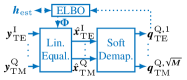
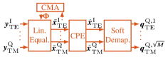
Fig. 1: Sketch of VAE (top) and CMA (bottom).

The widely-used equalizer for bootstrapping a coherent optical transmission system is the CMA [4]. In its common implementation [1], the distance of the equalized signal amplitude to the kurtosis of the transmitted constellation is minimized by updating the equalizer taps symbol-wise. By nature, the CMA is phase-insensitive and requires an additional carrier-phase estimation (CPE), where we apply the blind Viterbi-Viterbi algorithm [7] with a sufficient averaging over 501 symbols. Furthermore, there are variants of the CMA applying batch-wise updating via gradient descent (GD), e.g., as proposed in [8], which we denote as CMAbatch.

In comparison, we analyze the recently proposed VAE based equalizers [6], which use the evidence lower bound (ELBO) to approximate maximum likelihood (ML) channel estimation and, as a byproduct, equalize the received signal. The structures of both equalizer types are shown in Fig. 1. All algorithms update a similar linear equalizer block consisting of a complex-valued $2\times 2$ butterfly structure with finite impulse response (FIR) filters of length $M_{\mathrm{eq}}$, and we use a maximum a posteriori based soft demapper as in [9]. In fact, the VAE does not require a CPE and jointly updates—along with the equalizer taps—a similar but separate butterfly structure $\bm{h}_{\text{est}}$ of $M_{\mathrm{est}}$-long FIR filters for channel estimation. We use an Adam optimizer to update either batch-wise (VAEbatch) or with the VAEflex scheme as proposed in [6]. The latter is based on batch-wise processing, but instead of equalizing the whole batch per iteration, it only equalizes $N_{\text{flex}}<N_{\mathrm{batch}}$ symbols. In the next iteration, it equalizes the next $N_{\text{flex}}$ symbols, so it re-uses $N_{\mathrm{batch}}-N_{\text{flex}}$ symbols per iteration which boosts convergence. Further details can be found in [6]. We also propose the CMAflex scheme, which applies the same scheme based on the CMAbatch.

The batch-wise schemes consider a batch of $N_{\mathrm{batch}}=200$ symbols with learning rates of $\epsilon_{\mathrm{lr}}=$1.2\text{\cdot}{10}^{-4}$$ (CMAbatch) and $\epsilon_{\mathrm{lr}}=$2\text{\cdot}{10}^{-3}$$ (VAEbatch); the CMA uses $\epsilon_{\mathrm{lr}}=$8\text{\cdot}{10}^{-4}$$. The CMAflex/VAEflex schemes equalize $N_{\text{flex}}=10$ symbols while processing $N_{\mathrm{batch}}=100$ symbols per iteration, and use $\epsilon_{\mathrm{lr}}=$4.5\text{\cdot}{10}^{-5}$$ (CMAflex) and $\epsilon_{\mathrm{lr}}=$2\text{\cdot}{10}^{-3}$$ (VAEflex). All hyperparameters are optimized individually for each scheme to reduce the percentage of failed runs during bootstrapping.

Fig. 2: Results for different residual CD: the top plots correspond to unshaped $64$-QAM ($\mathcal{H}=6$), the bottom plots to PCS-$64$-QAM ($\mathcal{H}=5.73$). The inset constellation diagrams show the equalized signal after the VAEbatch at $L_{\mathrm{cd}}=$1.5\text{\,}\mathrm{km}$$. The plots on the right show the mean frame index $\bar{k}$ at which a threshold of $\text{BMI}_{\text{thr}}=5$ and $\text{BMI}_{\text{thr}}=4.8$ (for the PCS, respectively) is reached.

3 Simulation Environment

To analyze the bootstrapping of the different equalizers, we adapt the simulation environment of [6] (see also references therein) and use the same averaging scheme. Precisely, we transmit uniform $64$-QAM and PCS-$64$-QAM with an entropy of $\mathcal{H}=5.73$ bits per symbol (and a Maxwell-Boltzmann distribution), assume a time-invariant channel during the bootstrapping phase, and model the fiber by the linear frequency domain channel matrix

$$\bm{H}\left(f\right) =\bm{R}\begin{pmatrix}{\mathrm{e}}^{{\mathrm{j}}\pi\tau_{\text{pmd}}f}&0\\ 0&{\mathrm{e}}^{-{\mathrm{j}}\pi\tau_{\text{pmd}}f}\end{pmatrix}{\mathrm{e}}^{-{\mathrm{j}}2\pi^{2}\beta_{\text{cd}}L_{\text{cd}}f^{2}},\qquad\text{with}\quad\bm{R}=\begin{pmatrix}\cos\left(\gamma_{\text{hv}}\right)&\sin\left(\gamma_{\text{hv}}\right)\\ -\sin\left(\gamma_{\text{hv}}\right)&\cos\left(\gamma_{\text{hv}}\right)\end{pmatrix}\ ,$$

where $\bm{R}$ represents a static rotation of the reference polarization to the fiber’s principal state of polarization (PSP), called HV-phase-shift $\gamma_{\text{hv}}$. In contrast to [6], we do not consider the initial HV-phase-shift as compensated yet. Additionally, we include first-order polarization mode dispersion (PMD) caused by the differential group delay $\tau_{\mathrm{pmd}}$ between the PSPs, and residual CD, which is defined by the fiber’s group velocity dispersion (GVD) parameter $\beta_{\text{cd}}=-$26\text{\,}\mathrm{p}\mathrm{s}^{2}\mathrm{/}\mathrm{k}\mathrm{m}$$ (equals $D_{\text{cd}}=$20\text{\,}\mathrm{ps}\text{\,}{\mathrm{nm}}^{-1}\text{\,}{\mathrm{km}}^{-1}$$ at $\lambda=$1550\text{\,}\mathrm{nm}$$) times the uncompensated fiber length $L_{\mathrm{cd}}$. Complex AWGN is added on both polarizations.

We evaluate $N_{\text{ind}}=100$ frames ($N_{\text{ind}}=20$ for the VAEflex/CMAflex schemes) and apply the same averaging scheme as in [6], which results in an averaging over $80\,000\ldots 100\,000$ symbols per frame index and run. As performance metric, we use both the binary mutual information (BMI) (also often denotes as GMI) and the percentage of failed runs, which we define as runs where $\text{BMI}<5$ ($\text{BMI}<4.8$ for PCS with $\mathcal{H}=5.73$, respectively) after a sufficient number of samples. Similarly to [6], we apply a scheduler which halves the learning rate after every 20 (5 for the VAEflex/CMAflex schemes) frames for all algorithms.

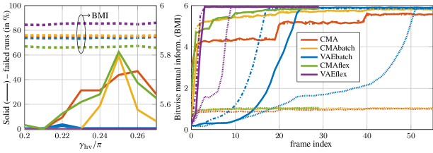
Fig. 3: Results for different initial HV-shift $\gamma_{\mathrm{hv}}$ (left), and the convergence behavior at $\gamma_{\mathrm{hv}}=$0.25$\pi$ (right), where the solid (—–) curve corresponds to the convergence of a typical run, the dotted ($\mathbf{\cdot\!\cdot\!\cdot\!\cdot\!\cdot\!}$) to the convergence of a bad run, and the dash-dotted ($\mathbf{\cdot-\cdot}$) to the convergence of a good run.

4 Numerical Results

All numerical results are simulated with $M_{\mathrm{eq}}=15$ and with a symbol rate of $R_{\text{S}}=$100\text{\,}\mathrm{G}\mathrm{B}\mathrm{d}$$, an oversampling factor of $N_{\text{os}}=2$  samples per symbol (sps), and an SNR of $24\text{\,}\mathrm{d}\mathrm{B}$ for uniform and $22\text{\,}\mathrm{d}\mathrm{B}$ for PCS-$64$-QAM with $\mathcal{H}=5.73$.

First, we analyze the convergence behavior at a challenging working point with $\gamma_{\mathrm{hv}}=$0.2$\pi$, $\tau_{\mathrm{pmd}}=\frac{T_{\text{S}}}{2}=\frac{1}{2R_{\text{S}}}$, and for various lengths $L_{\mathrm{cd}}$ of uncompensated fiber as depicted in Fig. 2. To take the potentially long channel impulse response into account, we use $M_{\mathrm{est}}=25$ taps. While the VAE equalizers achieve the highest BMI, the CMAbatch is the most stable algorithm for uniform QAM, where it converges reliably and within 5 frames as depicted in the right plot. The CMAflex/VAEflex converge as fast as the CMAbatch, but we observe a higher percentage of failed runs (left plots) for higher CD. However, the VAEflex achieves a significantly higher BMI than the CMAbatch and CMAflex. The computationally less expensive VAEbatch algorithm converges similarly reliably and equalizes well, as indicated by the constellation diagram in Fig. 2 as well as the high BMI. The bottom row depicts the results for moderately shaped PCS-64-QAM with an entropy of $\mathcal{H}=5.73$, which is commonly-known as challenging task for the popular CMA based blind equalizers. Only the VAE based equalizers, which consider the a priori density, converge reliably until the CD becomes too strong, while the CMAflex fails completely. The VAEflex is still converging within 10 frames but the VAEbatch converges more reliably.

At $\gamma_{\mathrm{hv}}=\frac{\pi}{4}$, the CMA’s loss function has a local minimum at an invalid constellation, so the left plot of Fig. 3 depicts a sweep of $\gamma_{\mathrm{hv}}$ around that point. We set a rather strong PMD with $\tau_{\mathrm{pmd}}=T_{\text{S}}$, a moderate $L_{\mathrm{cd}}=$1\text{\,}\mathrm{km}$$, and use $M_{\mathrm{est}}=15$. While the BMI after convergence stays similar (dashed), the percentage of failed runs (solid) increases significantly at $\gamma_{\mathrm{hv}}\approx\frac{\pi}{4}$ for all CMA based equalizers, which eventually fail in over 50% of the runs. However, the VAE based equalizers do not struggle at all for this working point. The right plot shows the convergence behavior at the critical point of $\gamma_{\mathrm{hv}}=\frac{\pi}{4}$. We chose three runs per algorithm representing a good (dash-dotted) and a bad (dotted) performance as well as typical curve (solid) of the converged runs. While the CMA based equalizers quickly reach a moderate BMI and converge slowly but gradually, the VAE based algorithms start at low BMI but converge rapidly. Hence, they reach their maximum BMI faster as all CMA based equalizers. The results show that all algorithms are significantly affected by the learning rate scheduler, which might be subject of further optimization.

5 Conclusion

We reveal critical working points in which the widely-used CMA and its variants fail to converge. The novel VAE based equalizers converge reliably at these critical points with both standard and PCS formats. The novel VAEflex is a fast-converging option and, for the CMA, we found that batch-wise updating is advantageous.

Acknowledgements: This work was carried out in the framework of the CELTIC-NEXT project AI-NET-ANTILLAS (C2019/3-3) and was funded by the German Federal Ministry of Education and Research (BMBF) under grant agreement 16KIS1316.

References

- [1] D. Godard, “Self-recovering equalization and carrier tracking in two-dimensional data communication systems,” IEEE Trans. Commun., vol. 28, no. 11, pp. 1867–1875, 1980.
- [2] M. Ready and R. Gooch, “Blind equalization based on radius directed adaptation,” in Proc. ICASSP, 1990.
- [3] F. P. Guiomar, S. B. Amado, A. Carena, G. Bosco, A. Nespola, A. L. Teixeira, and A. N. Pinto, “Fully blind linear and nonlinear equalization for 100G PM-64QAM optical systems,” J. Lightw. Technol., vol. 33, no. 7, pp. 1265–1274, 2015.
- [4] S. J. Savory, “Digital coherent optical receivers: Algorithms and subsystems,” IEEE J. Sel. Topics Quantum Electron., vol. 16, no. 5, pp. 1164–1179, 2010.
- [5] E. Zervas, J. G. Proakis, and V. Eyuboglu, “Effects of constellation shaping on blind equalization,” in Proc. SPIE, vol. 1565, 1991.
- [6] V. Lauinger, F. Buchali, and L. Schmalen, “Blind equalization and channel estimation in coherent optical communications using variational autoencoders,” IEEE J. Sel. Areas Commun., vol. 40, no. 9, pp. 2529–2539, 2022.
- [7] A. J. Viterbi and A. M. Viterbi, “Nonlinear estimation of PSK-modulated carrier phase with application to burst digital transmission,” IEEE Trans. Inf. Theory, vol. 29, no. 4, pp. 543–551, 1983.
- [8] D. E. Crivelli et al., “Architecture of a single-chip 50 Gb/s DP-QPSK/BPSK transceiver with electronic dispersion compensation for coherent optical channels,” IEEE Trans. Circuits Syst. I, vol. 61, no. 4, pp. 1012–1025, Apr. 2014.
- [9] J. Cho and P. J. Winzer, “Probabilistic constellation shaping for optical fiber communications,” J. Lightw. Technol., vol. 37, no. 6, pp. 1590–1607, 2019.