propagate: a seed propagation framework to compute Distance-based metrics on Very Large Graphs

Abstract

We propose propagate, a fast approximation framework to estimate distance-based metrics on very large graphs such as: the (effective) diameter or the average distance within a small error. The framework assigns seeds to nodes and propagates them in a BFS-like fashion, computing the neighbors set until we obtain either the whole vertex set (for computing the diameter) or a given percentage of vertices (for the effective diameter). At each iteration, we derive compressed Boolean representations of the neighborhood sets discovered so far. The propagate framework yields two algorithms: propagate-p, which propagates all the $s$ seeds in parallel, and propagate-s which propagates the seeds sequentially. For each node, the compressed representation of the propagate-p algorithm requires $s$ bits while propagate-s $1$ bit only. Both algorithms compute the average distance, the effective diameter, the diameter, and the connectivity rate (a measure of the the sparseness degree of the transitive closure graph) within a small error with high probability: for any $\varepsilon>0$ and using $s=\Theta\left(\frac{\log n}{\varepsilon^{2}}\right)$ sample nodes, the error for the average distance is bounded by $\xi=\frac{\varepsilon\Delta}{\alpha}$; the errors for the effective diameter and the diameter are bounded by $\xi=\frac{\varepsilon}{\alpha}$; and the error for the connectivity rate is bounded by $\varepsilon$ where $\Delta$ is the diameter and $\alpha$ is the connectivity rate. The time complexity of our approaches is $\mathcal{O}(\Delta\cdot m)$ for propagate-p and $\mathcal{O}\left(\frac{\log n}{\varepsilon^{2}}\cdot\Delta\cdot m\right)$ for propagate-s, where $m$ is the number of edges of the graph and $\Delta$ is the diameter.The experimental results show that the propagate framework improves the current state of the art in accuracy, speed, and space. Moreover, we experimentally show that propagate is also very efficient for solving the All Pair Shortest Path problem in very large graphs.

1 Introduction

The fast computation of distances between pairs of nodes in a graph is a fundamental task in network applications. Distance-based metrics are also used to compute different notions of centrality for nodes or edges that can be used to detect communities in very large graphs, as proposed by Girvan and Newman [26] or Fortunato et al. [25]. The diameter, i.e. the maximum distance between all reachable pairs in a graph, is an important parameter for analyzing graphs that, for example, change over the time [30], or real-world graphs as the web and social network graphs, which have small diameters [29] that shrink as they grow [33]. The fastest exact algorithm for computing the diameter of sparse graphs is based on solving the All-Pairs Shortest Paths (APSP) problem which, for unweighted graphs, can be computed by executing a Breadth-First Search (BFS) for each vertex, with a time complexity of $\Omega(mn)$, where $n$ is the number of nodes and $m$ the number of edges. For dense graphs, the best algorithm is based on matrix multiplication [19], which can be performed in time of $\tilde{\mathcal{O}}(n^{\omega})$, where $\omega<2.38$ [17, 41]. However, its well known that computing the diameter of a graph with $m$ edges requires $m^{2-o(1)}$ time under the Strong Exponential Time Hypothesis (SETH), which can be prohibitive for very large graphs [1, 20], so efficient approximation algorithms for diameter are highly desirable. A trivial $2$-approximation algorithm for the exact diameter in undirected graphs can be computed in $\mathcal{O}(m+n)$ time by means of a BFS-visit starting from an arbitrary node. A ${3}/{2}$-approximation algorithm was first presented by Aingworth et al. [2] with a time complexity of $\tilde{\mathcal{O}}(m\sqrt{n}+n^{2})$, further improved to $\tilde{\mathcal{O}}(m\sqrt{n})$ [38], and, with the same approximation ratio, to $\tilde{\mathcal{O}}(m^{3/2})$ or $o(n^{2})$, depending on the degree of sparsity of the graph [13]. If a graph is weakly connected, experiments with real-world graph data sets show that heuristics may decrease the average running time of the diameter computation [10]. The computation of the exact diameter is however susceptible to outliers. For this reason, it is preferable to use more robust metrics, such as the effective diameter, which is defined as the a percentile distance between nodes (e.g. $90^{th}$), i.e. the maximum distance that allows to connect that percentage of all reachable pairs [35, 39]. For large real graphs, even the exact computation of the effective diameter remains prohibitive since possible approaches are still based either on solving APSP or on computing a transitive closure. Also, some diameter approximation algorithms [10, 12] cannot be used to compute the effective diameter, that is because they are based on the computation of the greatest distances from the nodes that do not necessarily pass through all reachable pairs [10] or on merging the diameters independently computed on smaller subgraphs [12]. An alternative approach is to compute the neighborhood function to derive distance metrics. A neighborhood $N(u,r)$ is the set of all nodes reachable from the node $u$ by a path of length at most $r$. $N(u,r)$ is also known as the ball of center $u$ and radius $r$. The most efficient algorithms for approximating the effective diameter are based on the estimate of the size of neighborhoods. For example, ANF [36] is based on BFS and the use of Flajolet-Martin (FM) probabilistic counters [24], and HyperANF [7] is based on the same approach as ANF but with the use of HyperLogLog as probabilistic counter [21]. Cohen [16] uses an approach based on a non-probabilistic counter, that uses $k$ hash functions on neighborhoods by keeping only the minimum hash value (MinHash) for each hash function ($k$-mins sketches). When the hashing values are in the unit interval $[0,1]$, then it is possible to estimate $|N(u,r)|$ by means of the unbiased cardinality estimator $\frac{1}{\textrm{MinHash}\left(N(u,r)\right)}$, with the standard error a function of $k$. The MHSE framework [4], instead, uses the MinHash approach to derive dense representations (signatures) of large and sparse graphs that preserve similarity and thus providing an approximation of the size of the neighborhood of a node using the Jaccard similarity. ANF, HyperANF and MHSE are grounded on the observation that the size of $N(u,r)$ is sufficient to estimate the distance-based metrics.

Our contributions.

We propose a framework to estimate the distance-based metrics on graphs based on a mixed approach: sampling and counting. The core idea of our approach is to consider a small set of $s$ seed nodes and to count the nodes that can be reached by at least one of these seeds, that is, the size of the neighbourhood set at distance $d$. We define two implementations of our framework: propagate-p, and propagate-s. The time complexity of our approaches is, respectively, $\mathcal{O}(\Delta\cdot m)$, and $\mathcal{O}(s\cdot\Delta\cdot m)$, while the space complexity is $\mathcal{O}\left(s\cdot n+m\right)$, and $\mathcal{O}(n+m)$. We provide an estimate on the sample size needed to achieve a good estimate of the distance metrics up to a small error bound. More precisely, we prove that $s=\Theta(\frac{\log n}{\varepsilon^{2}})$ sample nodes are sufficient to estimate, with probability at least $1-\frac{2}{n^{2}}$: (1) the average distance with the error bounded by $\varepsilon\frac{\Delta}{\alpha}$; (2) both the effective diameter and the diameter with the error bounded by $\frac{\varepsilon}{\alpha}$; and, (3) the connectivity rate $\alpha$ with error bounded by $\varepsilon$, where $\alpha$ be the connectivity rate of the network (see Section 3 for the formal definition). It is important to underline that both the algorithms admit a straightforward and simple implementation in a fully distributed and parallel setting.

In Section 2, we give an overview of relevant results on approximation algorithms of distance based metrics. In Section 3 we provide some basic preliminaries to understand our work. In Section 4, we describe the core idea behind our novel framework, then we introduce the new algorithms propagate-p and propagate-s, and provide an unbiased error bound for the computation of the effective diameter, the diameter, the average distance, and the connectivity rate. In Section 5, we compare our framework with the state-of-the-art algorithms for approximating the distance-based metrics. Finally, in Section 6, we conclude and present future research directions.

2 Related Works

The literature on approximating distance-based metrics being vast, we restrict our attention to approaches that are closest to ours. We, thus, particularly focus on sampling and probabilistic techniques.

Estimating Diameter by Sampling.

There are three main questions to be addressed when sampling from large graphs [32]: how to sample nodes and edges, how to set a good sample size, how to evaluate the goodness of the sample, as well as the goodness of the chosen sampling method. In the case of undirected and connected graphs, the centrality of nodes can be estimated by sampling only $\mathcal{O}(\frac{\log n}{\varepsilon^{2}})$ nodes and compute all the distances to all other nodes, with an error of $\varepsilon\Delta$, where $\Delta$ is the graph diameter [22, 18], thus reducing the time complexity to $\mathcal{O}(\frac{\log n}{\varepsilon^{2}}\left(n\log n+m\right))$.

Estimating Diameter by Probabilistic Counters.

Palmer et al. proposed the ANF algorithm that exploits the (Flajolet-Martin) FM-counter [24] to derive the distance-based metrics of a graph. The core idea is to count the number of distinct nodes in each neighborhood $N(u,r)$, for all nodes $u$ and radius $r$. For each set $N(u,r)$, ANF yields a concatenation of $l$ bit-masks (sketches), where a bit-mask $l$ has probability $\frac{1}{2^{i+1}}$ of having the $i$-th bit set to $1$. An approximation of the number of distinct elements in a stream is derived by averaging the index of the least significant bit with value $0$ in each of the $l$ bitmasks, and is set to $\frac{2^{\textrm{mean}}}{0.77351}$ [24]. Building upon this approach, Boldi et al. [7] proposed HyperANF  that uses the HyperLogLog algorithm [21, 23] and improves ANF in terms of speed and scalability, providing a better estimate for the same amount of memory and number of passes. Although HyperLogLog is the best approximate data stream counting algorithm, it is known that it tends to overestimate the real size of small sets [27]. Empirical bias correction has been introduced in [27], where the correction works well in a good range of sizes, however errors persist on small sets where the LinearCounting algorithm [40], provides the best results. Alternatively, the MinHash technique can be used to estimate the size of the neighborhood with respect of All Distance Sketch (ADS) of a node of a weighted graph [15, 16]. For each node, an ADS consisting of the first $k$ MinHash is maintained. The estimate of the neighborhood of a node $u$ is given by hashing the nodes in the interval $[0,1]$ and filtering a node $v$ when its hash value is less than the $k$-th MinHash of the ADS, and when any other node in ADS is closer to $u$ than to $v$. This algorithm computes, for each pair $(u,v)$ the closeness similarity which generalizes the inverse probability of the MinHash estimate [6] with a Jaccard-like similarity function, that is $\frac{1}{max({\pi_{vx}},{\pi_{ux}})}$ in the case of $k=1$, where $\pi_{u,v}$ is the Dijkstra rank of $u$ with respect to the node $v$ according to the position of $u$ by increasing distance from $v$. If the graph is unweighted, then the BFS visit can be used and Cohen’s framework can be considered equivalent in the spirit to HyperANF but with the use of the MinCount probabilistic counter of [6] instead of HyperLogLog probabilistic counter. However, its implementation is very different from the one presented in [6] and does not yield a $O(m)$ space complexity as in [6]. Amati et al. proposed a different probabilistic approach based on the MinHash counter [4], and experimentally showed its superiority in comparison to HyperLogLog based counters. Another sketching and sampling based technique to model public-private social network graphs proposes to efficiently preprocess the public graph $G$ and to integrate it with a private user graph node in order to derive graph properties and measures [14].

3 Preliminaries

We proceed by formally introducing the terminology and concepts that we use in what follows. For $k\in\mathbb{N}$, we let $[k]=\{1,\dots,k\}$. An undirected graph is an ordered pair $G=(V,E)$, where $V$ is a set whose elements are called vertices or nodes, and $E$ is a set of unordered pairs of vertices, whose elements are called edges, or links or arcs. In a directed graph $G=(V,E)$, $E$ is a set of ordered pairs of vertices. Let $d(u,v)$ be the number of edges in the shortest path between $u$ and $v$. Given a graph $G=(V,E)$, define the neighborhood at distance at most $r$ for a node $u\in V$ as $N(u,r)=\{v\in V:d(u,v)\leq r\}$. Additionally, we define the neighborhood function at hop $r$ as the size of the set of pairs of nodes within distance $r$, formally: $|N(r)|=\left|\{(u,v)\in V\times V:d(u,v)\leq r\}\right|$. The diameter $\Delta$ of a graph is the longest shortest path in the graph. In terms of the neighborhood function we have: $\Delta=\min_{r\in[0,n-1]}\left\{r:\sum_{u}\left|N(u,r)\right|=\sum_{u}\left|N(u,r+1)\right|\right\}$. Similarly, the effective diameter is defined as $\Delta^{\texttt{eff}}=\min_{r\in[0,n-1]}\left\{r:\sum_{u}\left|N(u,r)\right|\geq\uptau\cdot\sum_{u}\left|N(u,\Delta)\right|\right\}$ for $\uptau\in[0,1]$. In this work, we consider $\uptau=0.9$, i.e. the $90^{th}$ percentile distance between the nodes. We can also evaluate the average distance of a graph $G=(V,E)$. Let $R(u,v)$ be the reachability function that assumes value $1$ if and only if $u$ can reach $v$ and $0$ otherwise. Thus we can write: $\texttt{AvgDist}=\frac{\sum_{u,v\in V}R(u,v)\cdot d(u,v)}{\sum_{u,v}R(u,v)}=\frac{\sum_{u}\sum_{r\in[\Delta]}\left(\left|N(u,r)\right|-\left|N(u,r-1)\right|\right)\cdot r}{\sum_{u}\left|N(u,\Delta)\right|}$. Observe that the number of reachable pairs can be also defined using the neighborhood function as: $\texttt{Nr.Reachable Pairs}=\left|N(\Delta)\right|$. Finally, we define the connectivity rate $\alpha$ of a graph as the sparseness degree of its transitive closure. $\alpha=\frac{1}{n\cdot(n-1)}\sum_{\begin{subarray}{c}u,v\\ u\neq v\end{subarray}}R(u,v)\in[0,1]$. Notice that the more the graph is connected the higher is $\alpha$, and vice versa. As extreme values $\alpha=1$ for a connected undirected graph, while $\alpha=0$ when all the vertices are isolated.

4 propagate Framework

Any graph traversal algorithm, efficiently scans the edge list of a graph in a random order. However, if the algorithm needs to be efficient on graphs that do not fit in memory, we can not use standard graph traversal routines. As in [36, 7, 4], we can find the nodes that are reachable from $u$ within $r$ hops by first retrieving their neighbors reachable in $r-1$ hops from $u$. Given $u$’s neighborhood at hop $0$, $N(u,0)=\{u\}$, we can compute $N(u,r)$ incrementally as: $N(u,r)=\bigcup_{(u,v)\in E}N(v,r-1)$. This technique allows to iterate over the edge set instead of performing a classical graph traversal. Probabilistic counters have been used to efficiently compute in terms of time and space the number of distinct elements in $N(u,r)$. The best known algorithms, namely HyperANF [7], and MHSE [4], use respectively the HyperLogLog [23] and the MinHash counter and drop the required memory down to $2\cdot s\cdot n\cdot\log_{2}(\log_{2}(n/s))$ bits and $2\cdot s\cdot n\cdot\log_{2}n$ (where $s$ is the number of seed nodes from which we are starting the edge scan procedure). Even though their performance are impressive, they turn out to be prohibitive on very large graphs if our memory budget is low. Our novel framework overcomes such problems by using a clever implementation of a boolean array-like data structure allowing to have high-quality approximations of the distance-based metrics on machines with low memory requirements. Given a set of starting nodes $S=\{x_{1},x_{2},\dots,x_{s}\}$, propagate  assigns to each node $u\in V$ a Boolean signature array $\texttt{Sig}(u)$ of length $s$ defined as follows: for all $i\in[s]$ $\texttt{Sig}_{i}(u)=\mathds{1}\left[u\in S\right]$, i.e., if the node $u$ is a seed, we set its coordinate to $1$. Next, we extend the concept of signature to a set of nodes of arbitrary size. Let $K\subseteq V$ be a subset of nodes, then its signature is defined as the bitwise OR between the signatures of every node $u\in K$, formally $\texttt{Sig}_{i}(K)=\bigvee_{u\in K}\texttt{Sig}_{i}(u)$ for every $i\in[s]$. Notice that the $i^{th}$ index of $\texttt{Sig}(K)$ is equal to $1$ if and only if there exists at least one vertex $u\in K$ such that $\texttt{Sig}_{i}(u)=1$. The intuition behind our boolean signature is as follows. Suppose that we have only one seed node $x$, by definition its signature will be of the form $\texttt{Sig}(x)=\langle 1\rangle$ i.e., $\texttt{Sig}_{1}(x)=1$. Subsequently, we expand the ball centered in $x$ to its hop-1 neighborhood and for each neighbor $v\in N(x)$ we create a new signature $\texttt{Sig}_{\texttt{new}}(v)$ equal to the bitwise OR between $\texttt{Sig}(x)$ and $\texttt{Sig}(v)$. After updating all $x$’s neighbors, for each $v\in N(x)$ we count the number of indices in its new signature that assumed value $1$ (one), we refer to the number of such indices as collisions between the seed’s bit and nodes’ signatures. The total number of ones will be equal to the size of $x$’s hop-1 neighborhood. Observe that such value can be efficiently computed by summing the number of ones obtained by performing the XOR (exclusive OR) operation between $\texttt{Sig}(v)$ and $\texttt{Sig}_{\texttt{new}}(v)$ for each neighbor $v$, formally $|N(x)|=\sum_{u\in V}\lVert\texttt{Sig}(u)\oplus\texttt{Sig}_{\texttt{new}}(u)\rVert$. If we iterate this process $\Delta$ times, we will compute the number of nodes at distance of exactly $r$ from $x$ for each $r\in[\Delta]$. By repeating this process $\Delta$ times for each node $x\in V$, we will obtain the exact neighborhood function $|N(r)|$ for each $r\in[\Delta]$. Recall that, under SETH, computing the exact neighborhood function cannot be done in $\mathcal{O}(n^{3-\varepsilon})$ for $\varepsilon>0$ [41], thus we run the propagate  framework on a subset of nodes $S$ sampled uniformly at random from $V$. Given a uniform sample of $s$ nodes from the vertex set $V$, the propagate framework can be implemented in two different ways: (1) every node has a signature of $s$ bits, and expands the $s$ balls (one for each seed node) in parallel until there is at least one signature that changed its value; (2) in a sequential fashion, every node spreads its bit until there is a signature that changed its value. We refer to these two implementations as propagate-p (Section  4.1), and propagate-s (Section  4.2). propagate-s is preferable to propagate-p when $s$ is very large and $s\cdot n$ bits becomes too big to be kept in the memory of a single machine. For example, when the set of seeds is the entire vertex set $V$, that is $s=|V|$, then propagate  computes the exact neighborhood function. To compute the ground-truth values, propagate-p  needs $n^{2}$-bit array that, for big graphs, can be too large to be stored on a single machine. propagate-s, instead, needs only $n$ bits. Thus, for this task, propagate-s is preferable to propagate-p . In Section 5.2 we compare the execution times of propagate-s  and the All Pair Shortest Path algorithm to compute the exact neighborhood function of big real-world graphs.

4.1 propagate-p Algorithm

Given $s$ sample nodes $\{x_{1},\dots,x_{s}\}\subseteq V$, propagate-p (Algorithm 1) works as a synchronous diffusion process. It starts by initializing (line 2-3) the signature $s$-array for each node $u\in V$, $\texttt{Sig}(u)$ as described in Section 4. Subsequently, at each hop $r$, it computes for each node $u$ the signature of the ball $N(u,r)=\{v\in V:d(u,v)\leq r\}$. The variable Count (line 5) keeps track of the number of new collisions at hop $r$, that is the number of vertices at distance exactly $r$ from $u$. The collisions at hop $r$ are subsequently stored in $\texttt{CountAll}[r]$ and if new collisions have been detected during the current hop, then the diameter lower-bound MaxHop is updated, the approximated neighborhood function at hop $r$ is computed ($R[r]$ contains the number of pairs at distance at most $r$), the variable AvgDist is increased with the difference between $R[r]$ and $R[r-1]$ times the hop $r$, and the hop $r+1$ is processed (lines 17-20). Once the stopping criterion is met, i.e. no more collisions have been detected, the algorithm finds the minimum hop $r$ such that the ratio between the reachable pairs at hop $r$ and at the maximum hop is greater than $90\%$ i.e., computes the effective diameter $\Delta^{\texttt{eff}}$ (line 21), and normalizes the average distance value by dividing it with the maximum number of reachable pairs (line 22). Algorithm propagate-p can be implemented using an array of $s$ bits for each vertex, thus we have the following theorem:

Theorem 4.1

Algorithm propagate-p (Algorithm 1) computes the: diameter, effective diameter, average distance and number of reachable pairs in $\mathcal{O}(\Delta\cdot m)$ time using $\mathcal{O}(s\cdot n+m)$ space.

Proof

After the initialization of the node signatures, at every step of the do-while, Algorithm  1 scans the graph by iterating over the nodes. During iteration $r$, if a node $u\in V$ has at least one of its $s$ signature bits set to $0$, it updates its signature by performing a bitwise OR between its signature and the one of its neighbors. Notice that, once a bit flips to $1$, it cannot go back to $0$. Subsequently, for each node $u\in V$ it counts the number of “bit-flips” occurred in the current iteration, and stores the value in CountAll$[r]$. The algorithm stops when the set of bits that change values to $1$ is empty. Notice that a seed $s$ can perform at most $n-1$ hops. Since, at every iteration of the do-while every seed is propagated in parallel (as a synchronous diffusion process), the algorithm iterates for at most $\Delta$ steps. Every iteration of the do-while requires at most $\mathcal{O}(m)$ steps. Thus, the time complexity of the loop is $\mathcal{O}(\Delta\cdot m)$. Subsequently, the algorithm computes the effective diameter. This can be done in linear time in the diameter of the graph $\Delta$. Algorithm  1, needs $s$ bits for each node signature, and two arrays of length $\Delta$ to store the number of collisions at each time step and the neighborhood function. Thus the space required by the algorithm is $\mathcal{O}\left(s\cdot n+m\right)$. The correctness of the algorithm follows from the definition of the propagate  framework in Section  4.

Data: $G=(V,E)\;:|V|=n$, $s$ sample of vertices $S\subseteq V$, eff. diameter threshold $\uptau$.

Result: $\Delta^{\texttt{eff}}$ effective diameter, $\Delta_{\texttt{LB}}$ diameter, $R[\Delta_{\texttt{LB}}]$ number of reach. pairs, and AvgDist average distance.

1

$\texttt{Sig}_{i}(u)=0;\quad\forall u\in V,i\in[s]$

  // $n\times s$ matrix of the nodes’ signature

2

3for each $x_{i}\in S$ do

4      

5      $\texttt{Sig}_{i}(x_{i})=1$

6$\texttt{CountAll}[0]=s,\texttt{Count}=0,\texttt{AvgDist}=0,\texttt{r}=0,\Delta_{\texttt{LB}}=0$

$\texttt{R}=[0,0,\dots,0]$

  // Neighborhood function

7

// Process one hop at a time for all the sample vertices $x_{i}$.

8 do

9      

      $\texttt{Count}=0$

        // Collision counter for hop $r$

10       foreach $u\in V$ do

11            

12            $\texttt{Sig}_{\texttt{next}}(u)=\texttt{Sig}(u)$

13            foreach  $\;u\rightarrow v$ do

14                   $\texttt{Sig}_{\texttt{next}}(u)=\texttt{Sig}_{\texttt{next}}(u)\vee\texttt{Sig}(v)$

15            

16      foreach $u\in V$ do

17             $\texttt{Count = Count}+\lVert\texttt{Sig}_{\texttt{next}}(u)\oplus\texttt{Sig}(u)\rVert$

            $\texttt{Sig}(u)=\texttt{Sig}_{\texttt{next}}(u)$

              // Update $u$’s signature

18            

19      

      $\texttt{CountAll}[r]=\texttt{Count}$

        // Reachable vertices at hop $r$

20      

      ${\Delta_{\texttt{LB}}}=\max{\{\texttt{r},\Delta_{\texttt{LB}}\}}$

        // Update diameter lower bound

21      

      $\texttt{R}[r]=R[r-1]+\texttt{CountAll}[r]$

        // $\texttt{R}[-1]$ treated as $0$ when $r=0$

22      

      $\texttt{AvgDist = AvgDist}+r\cdot(\texttt{R}[r]-\texttt{R}[r-1])$

        // $\texttt{R}[-1]$ treated as $0$ when $r=0$

23      

24      $\texttt{r = r}+1$

25while $\texttt{Count}>0$

$\Delta^{\texttt{eff}}=\min_{k}\left\{k:\frac{R[k]}{R[\Delta_{\texttt{LB}}]}\geq\uptau\right\}$

  // Compute the effective diameter ${\Delta^{\texttt{eff}}}$

26

$\texttt{AvgDist = AvgDist}/\texttt{R}[\Delta_{\texttt{LB}}]$

  // Compute the average distance

27

$R[\Delta_{LB}]=(n/s)\cdot R[\Delta_{LB}]$

  // Compute the number of reachable pairs

28

29return $\Delta^{\texttt{eff}}$,$\Delta_{\texttt{LB}}$,$\texttt{R}[\Delta_{\texttt{LB}}],\texttt{AvgDist}$

Algorithm 1 propagate-p Algorithm

4.2 propagate-s Algorithm

We derive an even more space efficient algorithm in which we process each sample vertex at a time using a single bit for each node in the graph, as with a Bernoulli process. propagate-s’s pseudo code, is presented in the extended version of this paper [5]. Differently from propagate-p which maintains a signature $s$-array for each vertex $u\in V$, propagate-s uses a $n$-array $\texttt{Sig}(V)$ that represents the signature of the whole graph $G=(V,E)$. More precisely, given a seed node $x_{i}$ $\texttt{Sig}(V)$, at each hop $r$, maintains the size of $x_{i}$’s neighborhood at distance at most $r$. Although, propagate-s has higher running time than propagate-p, the independence of the seeds in propagate-s allows for a very simple implementation of the algorithm in a fully distributed and parallel processing, where cores or machines can be coupled with hash functions. Additionally, propagate-s can be implemented using progressive sampling heuristics, that establish the sample size “on the fly” (see [5] for propagate-s’s incremental approach). When $s=|V|=n$, all propagate algorithms can compute the exact distance-based metrics of interest. In this case, propagate-p requires as signature a $n$ bit array for each vertex $u\in V$ thus requiring overall $n^{2}$ bits, which for large graphs is impracticable. However, propagate-s would require only a $n$-bit array at each iteration and can be used to compute the exact values for various graphs faster than the APSP algorithm implemented in WebGraph [8] (see Section 5). For huge graphs, the only feasible algorithm in a standalone setting is the propagate-s algorithm. The above considerations lead to the following theorem:

Theorem 4.2

propagate-s computes the: diameter, effective diameter, average distance and number of reachable pairs in $\mathcal{O}(s\cdot\Delta\cdot m)$ time using $\mathcal{O}(n+m)$ space.

Proof

The proof is similar to that of Algorithm  1. For each seed $s$, the algorithm scans the graph $\Delta$ times. Thus the time complexity is $\mathcal{O}(s\cdot\Delta\cdot m)$. In this case, the algorithm uses a signature of $n$ bits. Thus, the space complexity drops to $\mathcal{O}\left(n+m\right)$.

Data: $G=(V,E)\;:|V|=n$, $s$ sample of vertices $S\subseteq V$, eff. diameter threshold $\uptau$.

Result: $\Delta^{\texttt{eff}}$ effective diameter, $\Delta_{\texttt{LB}}$ diameter, $R[\Delta_{\texttt{LB}}]$ number of reach. pairs, and AvgDist average distance.

1

$\texttt{Sig}(u)=0;\quad\forall u\in V$

  // Graph’ signature

2

3$\texttt{CountAll}[0]=s,\texttt{Count}=0,\texttt{AvgDist}=0,\texttt{r}=0,\Delta_{\texttt{LB}}=0$

$\texttt{R}=[0,0,\dots,0]$

  // Neighborhood function

4

// Process each sample node $x_{i}$ at a time.

5 foreach $x_{i}\in S$ do

6      

      // Graph signature set to $1$ to the current sample node $x_{i}$ position, $0$ otherwise

7      

8      $\texttt{Sig}(x_{i})=1$

      $\texttt{Count}=0$

        // Initialize the collisions accumulator

9      

10      $\texttt{r}=0$

11      do

12            

13            NewSig = Sig

14            foreach $u\in V$ do

15                  

16                  if $\texttt{Sig}(u)=0$ then

17                         foreach $u\rightarrow v$ do

18                              

19                              $\texttt{NewSig(u) = NewSig(u)}\vee\texttt{{Sig}(v)}$

20                              if $\texttt{NewSig(u)}=1$ then

21                                    

22                                    Break;

23                              

24                        

25                  

26            

27            $\texttt{Count = Count}+\lVert\texttt{NewSig}\oplus\texttt{Sig}\rVert$

            ${\Delta_{\texttt{LB}}}=\max{\{\texttt{r},\Delta_{\texttt{LB}}\}}$

              // Update diameter lower bound

28             $\texttt{Sig}=\texttt{NewSig}$

29            $\texttt{CountAll}[r]=\texttt{CountAll}[r]+\texttt{Count}$

30            $\texttt{r = r}+1$

31      while $\texttt{Count}>0$

// Compute distance based metrics.

$\texttt{R}=[0,0,\dots,0]$ // It contains the overall reachable pairs at distance $\leq r$

32 for $k=0$ to $r-1$ do

33       $\texttt{R}[k]=\left(n\cdot\sum_{i\leq k}{\texttt{CountAll}[i]}\right)/s$

// Computation of the average distance

34

35for $k=0$ to $r-1$ do

36      

      $\texttt{AvgDist = AvgDist}+k\cdot(\texttt{R}[k]-\texttt{R}[k-1])$

        // $\texttt{R}[-1]$ treated as $0$ when $k=0$

37      

$\texttt{AvgDist = AvgDist}/R[\Delta_{\texttt{LB}}]$

  // Compute the average distance

38

$\Delta^{\texttt{eff}}=\min_{k}\left\{k:\frac{R[k]}{R[\Delta_{\texttt{LB}}]}\geq\uptau\right\}$

  // Compute the effective diameter ${\Delta^{\texttt{eff}}}$

39

40return $\Delta^{\texttt{eff}}$,$\Delta_{\texttt{LB}}$,$\texttt{R}[\Delta_{\texttt{LB}}],\texttt{AvgDist}$

41

Algorithm 2 propagate-s Algorithm

Error Bounds of the sample size.

We now evaluate the accuracy of the approximations of the propagate framework. We use Hoeffding’s inequality [28] to obtain the sample size $s$ for good approximations of the distance-based metrics of interest.

Theorem 4.3

With a sample of $s=\Theta\left(\frac{\ln n}{\varepsilon^{2}}\right)$ nodes, with high probability (at least $1-\frac{2}{n^{2}}$), propagate framework (propagate-p and propagate-s) compute:

• the average distance with the absolute error bounded by $\varepsilon\frac{\Delta}{\alpha}$

• the effective diameter with the absolute error bounded by $\frac{\varepsilon}{\tilde{\alpha}}$

• the diameter with the absolute error bounded by $\frac{\varepsilon}{\tilde{\alpha}}$

• the connectivity rate $\alpha$ with the absolute error bounded by $\varepsilon$

where $\tilde{\alpha}=\alpha\cdot\frac{n-1}{n}$, and $\varepsilon>0$ a positive constant. Thus, propagate-s requires $\mathcal{O}(\frac{\ln n}{\varepsilon^{2}}\cdot\Delta\cdot m)$ time and $\mathcal{O}(n+m)$ space . While, propagate-p requires $\mathcal{O}\left(n\frac{\log n}{\varepsilon^{2}}+m\right)$ space complexity.

Proof

Let us start with the average distance. Let $X_{i}=\frac{n\cdot\sum_{u}d(u,v_{i})\cdot R(u,v_{i})}{\sum_{u}\sum_{v}R(u,v)}$ with $\{v_{1},\dots,v_{s}\}\subseteq V$ a sample, where $X_{i}\in[0,\frac{\Delta}{\alpha}]$. The expectation of $X_{i}$ is the average distance:

$$\textbf{{E}}(X_{i})={\sum_{v_{i}\in V}X_{i}}\cdot{\textbf{{Pr}}(v_{i})}=\frac{\sum_{u}\sum_{v_{i}\in V}d(u,v_{i})\cdot R(u,v_{i})}{\sum_{u}\sum_{v_{i}\in V}R(u,v_{i})}$$ (1)

Then, Hoeffding’s inequality [28] generates the following bound:

$$\textbf{{Pr}}\left(\left|\frac{1}{s}\cdot\sum_{i=1}^{s}(\textbf{{E}}(X_{i})-X_{i})\right|\geq\xi\right)\leq 2\cdot\exp\left(\frac{-2s\xi^{2}\alpha^{2}}{\Delta^{2}}\right)$$ (2)

If $\xi=\varepsilon\frac{\Delta}{\alpha}$ then Equation 2 becomes:

$$\textbf{{Pr}}\left(\left|\frac{1}{s}\cdot\sum_{i=1}^{s}(\textbf{{E}}(X_{i})-X_{i})\right|\geq\varepsilon\frac{\Delta}{\alpha}\right)\leq 2\cdot\exp\left({-2s\varepsilon^{2}}\right)$$ (3)

Therefore it is sufficient to take $s=\Theta\left(\frac{\ln n}{\varepsilon^{2}}\right)$ to have, with high probability (at least $1-2\cdot\exp\left({-2\ln n}\right)=1-\frac{2}{n^{2}}$), an error at most $\varepsilon\frac{\Delta}{\alpha}$.

In a similar way we can derive error bounds for the effective diameter. Let $r$ be the effective diameter, and

$$X^{r}_{i}=\frac{\sum_{\{u:d(u,v_{i})\leq r\}}n\cdot R(u,v_{i})}{\sum_{u}\sum_{v}R(u,v)}=\frac{n\cdot|N(v_{i},r)|}{|N(\Delta)|}$$ (4)

where $X_{i}^{r}\in[0,\frac{1}{\tilde{\alpha}}]$, where $\tilde{\alpha}=\alpha\cdot\frac{n-1}{n}$ . Again, the expectation of the $X^{r}_{i}$ is:

$$\textbf{{E}}(X^{r}_{i})={\sum_{v_{i}\in V}X^{r}_{i}}\cdot{\textbf{{Pr}}(v_{i})}=\frac{\sum_{v_{i}\in V}|N(v_{i},r)|}{|N(\Delta)|}=\frac{|N(r)|}{|N(\Delta)|}$$ (5)

Applying Hoeffding’s inequality, with $\xi=\frac{\varepsilon}{\tilde{\alpha}}$, we approximate $\frac{|N(r)|}{|N(\Delta)|}$ by $\frac{\sum_{i=1}^{s}X^{r}_{i}}{s}=\displaystyle\frac{n\cdot\sum_{i=1}^{s}{|N(u,v_{i})|}}{s\cdot|N(\Delta)|}$ with a sample of $s=\frac{\ln n}{\varepsilon^{2}}$ nodes and an error bound of $\frac{\varepsilon}{\tilde{\alpha}}$, with high probability (at least $1-\frac{2}{n^{2}}$). Since the diameter $\Delta$ can be defined in terms of effective diameter $\min_{d^{\prime}}\left\{d^{\prime}:\frac{|N(d^{\prime})|}{|N(\Delta)|}\geq\tau\right\}$ by choosing $\tau=1$ instead of $0.9$, the effective diameter error bound holds also for the diameter. Finally, we give a bound for the number $|N(\Delta)|$ of reachable pairs. Since $|N(\Delta)|$ is a very large number we give the error bound for the ratio $\alpha=\frac{|N(\Delta)|}{n(n-1)}$. Let us define the random variable $X_{i}^{\Delta}=\frac{|N(v_{i},\Delta)|}{n-1}$ where $X_{i}^{\Delta}\in[0,1]$. The expected value of $X_{i}^{\Delta}$ is

$$\textbf{{E}}(X_{i}^{\Delta})=\sum_{v_{i}\in V}\frac{1}{n}\frac{|N(v_{i},\Delta)|}{n-1}=\frac{|N(\Delta)|}{n(n-1)}=\alpha$$ (6)

Applying Hoeffding’s inequality we approximate $\alpha$ with $s=\frac{\log n}{\varepsilon^{2}}$ and error bound of $\varepsilon$, with high probability (at least $1-\frac{2}{n^{2}}$).

In the following theorem we show that propagate and MHSE produce the same estimates. In other words, we can create a mapping between propagate’s signature and MHSE’ signature. This implies that the results in Theorem 4.3 can be extended to the MHSE Algorithm.

Theorem 4.4

Given a graph $G=(V,E)$ and a subset $S\subseteq V$ of $s$ seeds, propagate and MHSE produce the same set of reachable pairs $R[r]$ for $0\leq r\leq\Delta$.

Proof

It is sufficient to prove that both MHSE algorithm and propagate Algorithms produce the same set $R$ of of all reachable pairs at distance at most $r$. The key observation is that, for each collision with the minhash value of the graph for the MHSE Algorithm we have a collision in the signature $\texttt{Sig}(\cdot)$ for the propagate Algorithm and viceversa. Formally, let $\mathcal{H}$ be a set of $s$ hash functions over the nodes of the graph, and let $\texttt{Sig}_{MHSE}(\cdot)$ be the signature with the minhash values of the nodes over the $\mathcal{H}$ hash functions. Let $\mathcal{U}=\{u_{i}\}$ be the set of nodes that have the minimum hash values with $i\in\mathcal{H}$. We define $\texttt{Sig}_{i}(u)=1$ if and only if $u=u_{i}$. Viceversa, if we have a Boolean signature $\texttt{Sig}(\cdot)$ we may always define a signature $\texttt{Sig}_{MHSE}(\cdot)$ with $s$ hash functions having their minimum on the nodes with $\texttt{Sig}_{i}(u)=1$. At each hop and each hash function $i$, MHSE counts the number of source nodes for which the merge operation of their signatures with the signature of their target nodes produces a new collision (see Amati et al. [5] for more details), that is when $\texttt{Sig}_{MHSE}(u)$ becomes the minimum, that is when $u=u_{i}$, that is when $\texttt{Sig}_{i}(u)=1$, in other words, when there is a new collision for propagate. This show that the two Algorithms produce the same set of reachable pairs $R$ for each $0\leq r\leq\Delta$. Thus, they produce the same output.

5 Experimental Evaluation

In this section, we summarize the results of our experimental study on approximating the distance-based metrics in real-world networks. We compare our framework with the state-of-the-art algorithms to approximate the distance metrics, i.e., for each algorithm, we compute the average distance, effective diameter, and number of reachable pairs. Subsequently, we evaluate (using various metrics) how these estimates relates to the exact ones computed by the All Pairs Shortest Path algorithm.

5.1 Experimental Setting

Algorithms.

Our study includes several competitor algorithms for approximating the neighborhood function. We provide a short description and a space complexity analysis of the considered algorithms.

HyperANF:

The $\mathcal{O}(\Delta\cdot m)$ algorithm of Boldi et al. [7, 8], which uses HyperLogLog algorithms [21, 23] to approximate the neighborhood function. HyperANF  requires for each node $2^{b}=s$ registers that records the position $R$ with the bit $1$ starting the tail ending with all $0s$. More precisely, if $n$ is the number of distinct nodes in the graph, HyperANF needs $2\cdot s\cdot n\cdot\log_{2}\left(\log_{2}\left(n/s\right)\right)$ bits for the registers.

MHSE:

The $\mathcal{O}(\Delta\cdot m)$ algorithm of Amati et al. [4], which uses the MinHash counter to approximate the neighborhood function. MHSE is based on a BFS visit and it requires an $\mathcal{O}(\log n)$ register for each node to record the signature, hence, it has the same space complexity as ANF (ANF maintains a bitwise $\mathcal{O}(\log n)$ register to count new incoming nodes in the stream, instead). MHSE requires $2\cdot s\cdot n\cdot\log_{2}n$ bits.

rand-BFS:

The algorithm by Eppstein and Wang [22], which estimates the distance-based metrics using BFS visits starting from random nodes. Its time complexity is $\mathcal{O}(s\cdot m)$ and needs $\mathcal{O}(n+m)$ space.

APSP:

The Java implementation of the All Pair Shortest Path algorithm available in WebGraph[8]. The algorithm has been used to compute the exact values of the distance metrics and as a competitor algorithm for the second part of the experimental evaluation.

Networks

We evaluate all of the above competitors on real-world graphs of different nature, whose properties are summarized in Table 1. The networks come from two different domains: social networks and web-crawls. According to Theorem 4.3, the collection BlackFriday should require larger number of samples than other collections, because of a small connectivity rate (see Table  1).

Graph	n	m	$\bm{\Delta}$	$\bm{\alpha}$	Type	Ref.
BlackFriday	2700815	3811922	70	0.002	D	[3]
Youtube-Links	1138495	4942298	23	0.446	D	[31]
Amazon-2008	7600595	5158388	48	0.854	D	[9]
Web-BerkStan	685230	7600595	715	0.488	D	[34]
Twitch-Gamers	168114	13595114	8	1	U	[31]
Hollywood-2009	1139905	113891327	12	0.88	U	[9]
Orkut-2007	3072441	234370166	61	0.356	U	[9]
it-2004	41291594	1150725436	-	-	D	[9]
gsh-2015-host	68660142	1802747600	-	-	D	[9]
sk-2005	50636154	1949412601	-	-	D	[9]
gsh-2015	988490691	33877399152	-	-	D	[9]
clueweb12	978408098	42574107469	-	-	D	[9]
uk-2014	787801471	47614527250	-	-	D	[9]
eu-2015	1070557254	91792261600	-	-	D	[9]

Table 1: The data sets used in our evaluation, where $n$ denotes the number of nodes, $m$ the number of edges, $\Delta$ the exact diameter, $\alpha$ the exact connectivity rate (type D stands for directed and U for undirected). The first seven graphs have been used in comparison of the four algorithms (propagate, HyperANF,MHSE, and rand-BFS) for accuracy and effectiveness, and speed. The last seven have been used to compare the performances of the algorithms on huge graphs. Dashed lines indicate that the exact metrics are not available due to the dimension of the data set.

Implementation and Evaluation details.

We released an open source platform for analyzing large graphs. This tool is developed in Java and uses some WebGraph libraries [8] to load and parse the graph in compressed form. We chose WebGraph both for benchmarking with the compared algorithms and to allow us to: (1) compress very large graphs; (2) iterate the neighbor list of a node with faster random access; and, (3) use its offline methods to process very big graphs that cannot be loaded in memory. We executed the experiments on a server running Ubuntu 16.04.5 LTS equipped with AMD Opteron 6376 CPU (2.3GHz) for overall 32 cores and 64 GB of RAM. All the algorithms are fairly compared, i.e. using the same number of seeds/registers and cores. For the comparison between propagate, HyperANF, MHSE, and rand-BFS we use 256 sample nodes/registers and 32 cores. For the comparison between propagate-s and APSP we use 32 cores. For the first part of the experiments, we repeat every test $10$ times and average over the results for every algorithm (HyperANF, MHSE, rand-BFS, propagate-p, and propagate-s). Whenever we are able to compute the exact value $\hat{x}$ and thus the residual $(\hat{x}-\tilde{x})/\hat{x}$ where $\tilde{x}$ its estimate we also exhibit a p-value. More precisely, we perform a two-sided unpaired t-test [11] with confidence interval of $0.95$. Given a set $X$ of estimates of the distance metric $y$ obtained after $10$ runs of an algorithm $\mathcal{A}$, the null hypothesis is that its mean $\overline{X}$ is equal to the exact value $X$. If the displayed p-value is in the range $[0.9,1.0]$ then we fail to reject the null hypothesis, and conclude that the means are not significantly different. Therefore, we can conclude that algorithm $\mathcal{A}$ provides reliable and statistically significant estimates of $y$.

5.2 Experimental Results

Accuracy and effectiveness

In our first experiment, we run on the networks listed in the first group of Table 1 all the discussed approximation algorithms. In Table 4, we show the accuracy and effectiveness of all the competitor algorithms. propagate-p and propagate-s are grouped under the name of propagate, that is because both algorithm produce the same results. We observe that our novel framework leads the scoreboard against its competitors. It provides the best estimations in terms of accuracy and statistical significance. For the average distance, propagate outperforms all the other algorithms on all the graphs except on Orkut, in which rand-BFS provides the best estimate. Moreover, it provides the best effective diameter estimates on all the datasets. Finally, for the number of reachable pairs, propagate provides very accurate estimations on all the networks except on Youtube for which MHSE’s estimate has lower residual. Observe that propagate  is the algorithm that provides the higher number of statistically significant estimations and does not perform worse than the competitor algorithms.

Speed.

As a second experiment, we compared the average execution times of propagate-p, propagate-s, HyperANF, MHSE, and rand-BFS. In the left side of Table 2, we show the running times (in milliseconds) of the algorithms. We observe that propagate  framework outperform its competitors on almost every data set. Remarkably, propagate-p, leads the scoreboard with the fastest execution times on four over seven graphs. It is slightly slower than rand-BFS on balckFriday, Amazon-2008, and Web-BerkStan i.e. the datasets with low connectivity rate and longest diameters for which a classic traversal algorithm should require less time than our framework. We point out that, rand-BFS does not scale well as the size of the graph increases (as shown in the next experiment). We observe that, on average, propagate-p  is $60\%$ faster than HyperANF  and $81\%$ faster than MHSE. Moreover, propagate-p  outperform (in terms of speed) HyperANF, and MHSE on all the graphs. HyperANF’s execution time is comparable with the one of propagate-s while MHSE is the slowest one. More precisely, MHSE is slower than every other algorithm on every network for which it does not require more than $64GB$ or RAM i.e., does not generate a memory overflow error.

	Execution time
	Milliseconds					Hours
Graph	Prop-P	Prop-S	HyperANF	MHSE	Rand-BFS	Prop-S	APSP
b.Friday	282.162	2899.075	22495.344	51034.047	69.21	9.513	33.705
YT-Links	1761.891	5040.347	5986.410	6655.706	1771.25	7.217	11.118
Amazon	4339.072	12686.703	8451.259	195200.019	1767.12	11.027	11.914
W.Berk.	1535.781	2477.531	2741.563	5980.219	645.25	33.108	122.59
Twitch-G.	1562.219	2901.497	2288.231	4486.044	1863.10	0.344	3.617
Hollywood	4113.060	15537.897	11068.953	46409.728	7672.18	47.77	158
Orkut	2875.688	8121.125	3833.688	✗	12783.13	840	960

Table 2: For each network (column 1), we show on the left side of the table the average execution time (in milliseconds) over ten runs for each algorithm. On the right side, we show the execution time (in hours) of propagate-s, versus WebGraph’s APSP algorithm to compute the ground truth distance-based metrics. ✗  indicates that the experiment was interrupted due to a memory overflow error.

Estimating Distance Metrics on huge graphs.

As a third experiment, we run all the approximation algorithms on the biggest networks available in [9] (see the second group of data sets in Table 1). We aim to to investigate the performances of all the competitor algorithms on very big graphs that cannot be loaded in the main memory. In Table  3, we show the running times of the approximation algorithms. The first column indicates whether the graph can be fully loaded in memory in its uncompressed form. If this is not possible, we use WebGraph’s offline methods to access the compressed graph from the disk without loading it in memory. Observe that accessing the compressed graph directly from the disk, slows down the overall execution of the algorithms. However, it is the only way to analyze these graphs with our $64$GB memory machines. We observe that propagate-s can compute the distance metrics on every graph. Considering the size of the data sets, propagate-s requires a reasonable amount of time to approximate the neighborhood function using $256$ seeds. propagate-p can compute the distance metrics for it-2004, gsh-2015-host, and sk-2005. Moreover, it is still possible to run propagate-p on the remaining graphs by appropriately decreasing the number of sample nodes. Instead, HyperANF can be used only to compute the approximated neighborhood function only on it-2004, and sk-2005. Finally, MHSE and rand-BFS cannot be used on any of these networks. Before comparing the time performances, we point out that the red dash ( –) in Table 3 indicates that the algorithm requires more than $64$GB of memory even with $1$ seed/register. Thus, decreasing the number of seeds/registers is not enough to run these algorithms on these huge networks, we would need to upgrade the RAM of the machine. From the results in Table 3, we observe that (on it-2004, and sk-2005) propagate-p is on average $64\%$ faster than HyperANF. Furthermore, propagate-s is the best algorithm to approximate the neighborhood function on huge data sets. It requires $n\cdot s$ bits, to store the graph signature. Indeed, for eu-2015, i.e. the biggest graph in Table 1, it needs approximately at most $1$GB to store the graph signature. Thus, using WebGraph’s offline methods to scan the graph, propagate-s could provide the approximated neighborhood function of eu-2015 using an average laptop.

		Execution Time
Graph	In memory	Propagate-P	Propagate-S	HyperANF	MHSE	rand-BFS
it-2004	Yes	33.26 minutes	52.13 minutes	62.18 minutes	–	–
gsh-15-h	No	40 minutes	4.16 hours	–	–	–
sk-2005	Yes	44 minutes	6 hours	4 hours	–	–
gsh-2015	No	✗	11 hours	–	–	–
clueweb12	No	✗	9.56 hours	–	–	–
uk-2014	No	✗	39 hours	–	–	–
eu-2015	No	✗	7 days	–	–	–

Table 3: For each network (column 1), we show the loading method (column 2) “Yes” means that it is possible to load the entire graph in memory, while “No” indicates that is not possible. In such a case, we use WebGraph’s offline methods to iterate trough the successor lists. For each algorithm, we show the execution time (using $256$ seeds/registers). ✗  indicates that the experiment was interrupted due to a memory overflow error of the algorithm while initializing the signature/registers array. Here, the red dash – indicates that the algorithm cannot run even with $1$ seed/register.

Computing ground truth metrics with propagate.

As a last experiment, we compare propagate-s with the WebGraph implementation of the All Pair Shortest Path (APSP) algorithm to compute the exact neighborhood function. Among all the competitor algorithms, HyperANF cannot be used to compute the ground truth values of a graph. That is because its neighborhood function estimator that uses the HyperLogLog counter is asymptotically almost unbiased [7]. MHSE instead, cannot be employed because of its high space complexity. Observe that rand-BFS coincides with WebGraph’s APSP algorithm. As showed in the proof of Theorem 4.3 (see [5]) propagate’s distance metrics estimators are all unbiased. Thus, our novel framework can be used to compute the ground truth values. Given a $n$ vertices graph $G=(V,E)$, propagate suffices of the entire vertex set $V$ as set of seeds to compute the exact distance metrics. For this experiment, we use propagate-s because it needs only $n$ bits to store the graph signature, while propagate-p would need $n^{2}$ bits and with a $64$GB machine can be used only for computing the ground truth metrics of the first three graphs in Table 1. In the right side of Table 2, we show the running times of propagate-s and APSP. We observe that propagate-s is faster than WebGraph’s APSP implementation on all the data sets. These results suggest that our implementation of propagate-s is preferable for retrieving exact values of distance-based metrics on very large real-world graphs.

propagate-s’s incremental approach.

In this experiment, we aim to better investigate the dependency of propagate’s performance with respect to its sample size. We recall that Theorem 4.3 states that a sample of $\mathcal{O}(\log n)$ nodes is enough to obtain good approximations of the average distance and the effective diameter with high probability, although $256$ seeds give really good approximations (see Table  4). Figure 1, shows the performances of the propagate framework with a representative increasing number of seeds, that is $s=16,64,256$. propagate achieves high quality approximations with $64$ seeds even for Orkut-2007 and Web-BerkStan i.e. the graphs that have low connectivity rate $\alpha$. Our novel framework performs well for each approximation (average distance, effective diameter, and number of reachable pairs) with $64$ seeds on both directed and undirected graphs. Figure 1 (c) shows the effectiveness of the framework as a probabilistic counter of the set of reachable nodes for both, directed and undirected graphs. Therefore, propagate-s can be used with a progressive sampling approach [37]. Indeed we could start with a small sample of nodes and progressively increase it if a certain stopping criterion is not met yet, allowing for an even faster approximation approach.

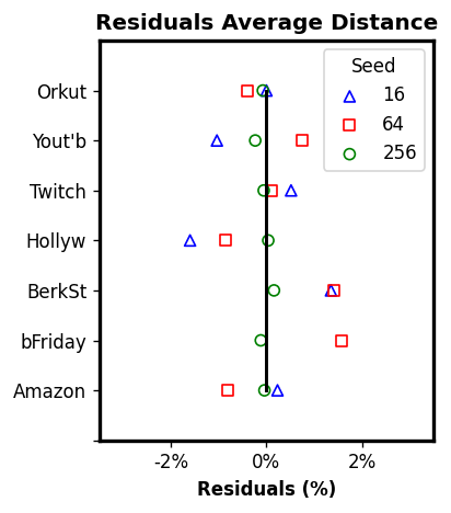
(a)

(b)

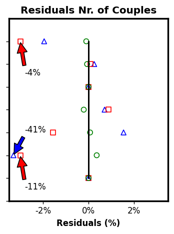
(c)

Figure 1: Effectiveness of propagate on real world graphs with different number of seeds. Plots of the residuals for: Average Distance, Effective Diameter at 90% , and Number of Connected Pairs.

6 Conclusions

We proposed propagate, a novel framework for estimating distance-based metrics on very large graphs. In Section 4, we provided two different implementation of our framework, that, so far, can approximate: average distance, (effective) diameter, and the connectivity rate up to a small error with high probability. Our experimental results are summarized in Section 5.1, which depicts the performance of our framework versus the state-of-the-art algorithms. Our approach over-perform in terms of accuracy and running time all its competitors. Moreover, when applied to very large real-world graphs, propagate-s (and propagate-p if applicable) clearly outperforms all the other algorithms in terms of scalability. As indicated in Table 3, our framework is the only available option to approximate distance-based metrics when we do not have access to servers with a large amount of memory. In the spirit of reproducibility, we developed an open source framework in Java that allows any user with an average laptop to approximate the distance-based metrics considered in this paper on any kind of graph. Some promising future directions are to use propagate to compute centrality measures on vertices and edges, and to extend our framework to community detection tasks.

Acknowledgements.

This work was partially supported by the European Union under the Italian National Recovery and Resilience Plan (NRRP) of NextGenerationEU, partnership on “Telecommunications of the Future” (PE00000001 program “RESTART”)

		Neighborhood Function Estimation
					Residual/$\hat{x}$ (p-value)
Graph	Algo.	Av. Dist.	Eff. Diam. 90	Nr. of conn pairs	Av. Dist.	Eff. Diam. 90	Nr. of conn pairs
blackFriday	Exact$(\hat{x})$	16.124	22.722	11,300,563,035
	prop.	16.143	22.551	11,259,575,354	-0.001(0.92∙)	-0.008(0.95∙)	0.003(0.72)
	H.ANF(▲)	16.214	22.841	11,032,542,659	0.01(0.26)	0.005(0.40)	-0.024(0.34)
	MHSE	16.338	23.029	12,193,068,803	-0.01(0.12)	-0.01(0.23)	-0.07(0.09)
	rnd-BFS	17.381	24.30	8,636,102,833	-0.078(0.60)	-0.069(0.68)	0.24(0.09)
Youtube	Exact$(\hat{x})$	5.104	6.244	577,863,455,179
	prop.	5.104	6.291	578,216,139,787	0(1∗∗)	-0.007 (0.44)	-6e-4 (0.73)
	H.ANF	5.131	6.301	602,314,527,291	-0.005 (0.1)	-0.009 (0.11)	-0.042 (0.1)
	MHSE	5.105	6.165	577,569,359,888	0.003(0.25)	0.013(0.08)	5e-4(0.65)
	rnd-BFS	5.11	6.217	579,121,217,963	-0.001(0.72)	0.004(0.60)	-0.002(0.01)
Amazon	Exact$(\hat{x})$	12.075	15.544	461,523,315,650
	prop.	12.08	15.519	461,523,315,650	0.00(0.93∙)	-0.002(0.80)	0.00(1∗∗)
	H.ANF	12.042	15.47	451,448,606,322	-0.003(0.44)	-0.022(0.31)	-0.022(0.31)
	MHSE	12.1	15.542	462,552,552,254	-0.002(0.54)	1e-4(0.98∗)	-0.002(0.65)
	rnd-BFS	12.103	15.579	461,522,729,233	-0.002(0.36)	-0.002(0.53)	1.27e-6(0.05)
BerkStan	Exact$(\hat{x})$	13.905	17.777	229,179,533,137
	prop.	13.883	17.777	229,015,123,311	0.02(0.42)	0(1∗∗ )	7e-4(0.65)
	H.ANF	14.645	17.728	233,108,112,819	0.053(0.40)	-0.003(0.83)	0.017(0.49)
	MHSE	15.29	18.14	239,485,315,387	0.099(0.61)	0.02(0.61)	0.045(0.36)
	rnd-BFS	14.341	18.02	228,188,757,612	-0.031(0.44)	-0.02(0.28)	0.004(0.80)
Twitch	Exact$(\hat{x})$	2.876	3.127	28,262,316,996
	prop.	2.876	3.129	28,262,316,996	0.0(1∗∗)	-0.001 (0.94∙)	0.00(1.00∗∗)
	H.ANF	2.891	3.180	28,451,734,342	-0.005 (0.03)	-0.017 (0.06)	-0.007 (0.78)
	MHSE	2.881	3.140	28,262,316,996	-0.002(0.44)	-0.001(0.62)	0.00(1.00∗∗)
	rnd-BFS	2.868	3.096	28,262,020,235	0.0027(0.33)	0.01(0.29)	1e-5(0.01)
Hollywood	Exact$(\hat{x})$	3.855	4.394	1,143,030,619,175
	prop.	3.855	4.397	1,143,485,513,294	-2e-4(0.92∙)	-3.9e-4(0.95∗)	-8e-4(0.90∙)
	H.ANF	3.848	4.374	1,136,104,164,355	0.16(0.49)	-0.46(0.5)	0.61(0.80)
	MHSE	3.857	4.382	1,138,248,927,314	-3.91e-4 (0.86)	0.003 (0.65)	0.0042(0.56)
	rnd-BFS	3.840	4.364	1,143,960,403,951	0.004(0.18)	0.007(0.16)	-0.001(0.90∙)
Orkut	Exact$(\hat{x})$	6.397	8.906	3,359,893,990,935
	prop.	6.402	8.895	3,386,716,107,589	-7e-4(0.90∙)	0.001(0.82)	-0.008(0.60)
	H.ANF	6.389	8.917	3,336,311,224,217	0.001(0.53)	-0.001(0.76)	0.01(0.45)
	MHSE	✗	✗	✗	✗	✗	✗
	rnd-BFS	6.399	8.929	3,328,105,314,542	-4e-4(0.91∙)	-0.003(0.61)	0.01(0.32)

Table 4: The comparison of HyperANF, propagate, and MHSE using 10 trials and 256 registers and 256 sample nodes respectively. Statistical significance at the $90\%$, $95\%$ and $99\%$ confidence level are marked with ^∙, * and ** respectively. The algorithms requiring more heap size are marked with ^▲ , and ✗  indicates that the algorithm needs more than $64$GB of memory.

References

- [1] Abboud, A., Williams, V.V.: Popular conjectures imply strong lower bounds for dynamic problems. In: 55th IEEE Annual Symposium on Foundations of Computer Science, FOCS 2014, Philadelphia, PA, USA, October 18-21, 2014. IEEE Computer Society (2014)
- [2] Aingworth, D., Chekuri, C., Indyk, P., Motwani, R.: Fast estimation of diameter and shortest paths (without matrix multiplication). SIAM Journal on Computing 28(4), 1167–1181 (1999). https://doi.org/10.1137/S0097539796303421
- [3] Amati, G., Angelini, S., Capri, F., Gambosi, G., Rossi, G., Vocca, P.: Modelling the temporal evolution of the retweet graph. IADIS International Journal on Computer Science & Information Systems 11(2, ISSN: 1646-3692), 19–30 (2016)
- [4] Amati, G., Angelini, S., Gambosi, G., Rossi, G., Vocca, P.: Estimation of distance-based metrics for very large graphs with minhash signatures. In: Proceedings of 2017 IEEE International Conference on Big Data. IEEE (Dec 11-14 2017)
- [5] Amati, G., Cruciani, A., Pasquini, D., Vocca, P., Angelini, S.: propagate: a seed propagation framework to compute distance-based metrics on very large graphs. CoRR (2023). https://doi.org/10.48550/arXiv.2301.06499
- [6] Bar-Yossef, Z., Jayram, T.S., Kumar, R., Sivakumar, D., Trevisan, L.: Counting distinct elements in a data stream. In: Proc. 6th Int. Work. on Random. and Approx. Tech. in Comp. Sc. pp. 1–10. Cambridge, MA (2002)
- [7] Boldi, P., Rosa, M., Vigna, S.: HyperANF: Approximating the neighbourhood function of very large graphs on a budget. In: Proc. 20th International Conference on World Wide Web. pp. 625–634. Hyderabad, India (2011)
- [8] Boldi, P., Vigna, S.: The WebGraph framework I: Compression techniques. In: Proc. of the Thirteenth International World Wide Web Conference (WWW 2004). pp. 595–601. ACM Press, Manhattan, USA (2004)
- [9] Boldi, P., Vigna, S.: LAW Datasets: Laboratory for web algorithmics. https://law.di.unimi.it/datasets.php (Apr 2022)
- [10] Borassi, M., Crescenzi, P., Habib, M., Kosters, W.A., Marino, A., Takes, F.W.: Fast diameter and radius BFS-based computation in (weakly connected) real-world graphs. Theor. Comp. Sc. 586, 59–80 (2015)
- [11] Casella, G., Berger, R.: Statistical Inference. Duxbury Resource Center (2001)
- [12] Ceccarello, M., Pietracaprina, A., Pucci, G., Upfal, E.: Distributed graph diameter approximation. Algorithms 13, 216 (09 2020). https://doi.org/10.3390/a13090216
- [13] Chechik, S., Larkin, D.H., Roditty, L., Schoenebeck, G., Tarjan, R.E., Williams, V.V.: Better approximation algorithms for the graph diameter. In: Proceedings of the Twenty-fifth Annual ACM-SIAM Symposium on Discrete Algorithms. pp. 1041–1052. SODA ’14, Society for Industrial and Applied Mathematics, Philadelphia, PA, USA (2014), http://dl.acm.org/citation.cfm?id=2634074.2634152
- [14] Chierichetti, F., Epasto, A., Kumar, R., Lattanzi, S., Mirrokni, V.S.: Efficient algorithms for public-private social networks. In: Proceedings of the 21th ACM SIGKDD International Conference on Knowledge Discovery and Data Mining, Sydney, NSW, Australia, August 10-13, 2015 (2015)
- [15] Cohen, E.: Size-estimation framework with applications to transitive closure and reachability. J. Comput. Syst. Sci. 55(3), 441–453 (1997)
- [16] Cohen, E.: All-distances sketches, revisited: Hip estimators for massive graphs analysis. In: Proc. 33rd ACM SIGMOD-SIGACT-SIGART Symp. on Princ. of Database Systems. pp. 88–99. Snowbird, Utah, USA (2014)
- [17] Coppersmith, D., Winograd, S.: Matrix multiplication via arithmetic progressions. Journal of Symbolic Computation 9(3), 251 – 280 (1990)
- [18] Crescenzi, P., Grossi, R., Lanzi, L., Marino, A.: A comparison of three algorithms for approximating the distance distribution in real-world graphs. In: Theory and Practice of Algorithms in (Computer) Systems - First International ICST Conference, TAPAS 2011, Rome, Italy, April 18-20, 2011. Proceedings. Lecture Notes in Computer Science, Springer (2011)
- [19] Cygan, M., Gabow, H.N., Sankowski, P.: Algorithmic applications of baur-strassen’s theorem: Shortest cycles, diameter, and matchings. J. ACM 62(4), 28:1–28:30 (2015). https://doi.org/10.1145/2736283, http://doi.acm.org/10.1145/2736283
- [20] Dalirrooyfard, M., Wein, N.: Tight conditional lower bounds for approximating diameter in directed graphs. In: STOC ’21: 53rd Annual ACM SIGACT Symposium on Theory of Computing, Virtual Event, Italy, June 21-25, 2021. ACM (2021)
- [21] Durand, M., Flajolet, P.: Loglog counting of large cardinalities (extended abstract). In: Proc. 11th Ann. Europ. Symp. (ESA). pp. 605–617. Budapest (2003)
- [22] Eppstein, D., Wang, J.: Fast approximation of centrality. In: Proc. 12th Ann. ACM-SIAM Symp. on Discrete Algorithms. pp. 228–229. Washington, D.C., USA (2001)
- [23] Flajolet, P., Fusy, É., Gandouet, O., Meunier, F.: Hyperloglog: The analysis of a near-optimal cardinality estimation algorithm. In: Analysis of Algorithms. pp. 137–156. Disc. Math. and Theor. Comp. Sc. (2007)
- [24] Flajolet, P., Martin, G.N.: Probabilistic counting algorithms for data base applications. J. Comput. Syst. Sci. 31(2), 182–209 (1985)
- [25] Fortunato, S., Latora, V., Marchiori, M.: Method to find community structures based on information centrality. Phys Rev E Stat Nonlin Soft Matter Phys 70(5 Pt 2), 056104 (Nov 2004). https://doi.org/10.1103/PhysRevE.70.056104
- [26] Girvan, M., Newman, M.E.J.: Community structure in social and biological networks. Proceedings of the National Academy of Sciences 99(12), 7821–7826 (2002). https://doi.org/10.1073/pnas.122653799, https://www.pnas.org/content/99/12/7821
- [27] Heule, S., Nunkesser, M., Hall, A.: Hyperloglog in practice: Algorithmic engineering of a state of the art cardinality estimation algorithm. In: Proc. 16th Int. Conf. on Ext. Datab. Tech. (EDBT). pp. 683–692. Genoa (2013)
- [28] Hoeffding, W.: Probability inequalities for sums of bounded random variables. In: The collected works of Wassily Hoeffding. Springer (1994)
- [29] Kleinberg, J.: The small-world phenomenon: An algorithmic perspective. In: Proceedings of the Thirty-second Annual ACM Symposium on Theory of Computing. pp. 163–170. STOC ’00, ACM, New York, NY, USA (2000). https://doi.org/10.1145/335305.335325, http://doi.acm.org/10.1145/335305.335325
- [30] Kumar, R., Novak, J., Tomkins, A.: Structure and evolution of online social networks. In: Proc. 12th ACM SIGKDD Int. Conf. on Knowledge Discovery and Data Mining. pp. 611–617. Philadelphia, PA, USA (2006)
- [31] Kunegis, J.: KONECT – The Koblenz Network Collection. In: Proc. Int. Conf. on World Wide Web Companion (2013)
- [32] Leskovec, J., Faloutsos, C.: Sampling from large graphs. In: Proc. 12th Int. Conf. ACM SIGKDD. pp. 631–636. Philadelphia, PA, USA (2006)
- [33] Leskovec, J., Kleinberg, J., Faloutsos, C.: Graphs over time: Densification laws, shrinking diameters and possible explanations. In: Proc. 11th Int. Conf. ACM SIGKDD. pp. 177–187. Chicago, IL, USA (2005)
- [34] Leskovec, J., Krevl, A.: SNAP Datasets: Stanford large network dataset collection. http://snap.stanford.edu/data (Jun 2014)
- [35] Palmer, C., Siganos, G., Faloutsos, M., Faloutsos, C., Gibbons, P.: The Connectivity and Fault-Tolerance of the Internet Topology. In: Proc. Work. on Network-Related Data Manag. vol. 25. S. Barbara, USA (2001)
- [36] Palmer, C.R., Gibbons, P.B., Faloutsos, C.: Anf: A fast and scalable tool for data mining in massive graphs. In: Proc. 8th ACM SIGKDD Int. Conf. on Knowledge Discovery in Data Mining. pp. 81–90. ACM (2002)
- [37] Riondato, M., Upfal, E.: Mining frequent itemsets through progressive sampling with rademacher averages. In: Proceedings of the 21th ACM SIGKDD International Conference on Knowledge Discovery and Data Mining (2015)
- [38] Roditty, L., Williams, V.V.: Fast approximation algorithms for the diameter and radius of sparse graphs. In: Proc. 45th Symposium on Theory of Computing (STOC). pp. 515–524. Palo Alto, CA, USA (2013)
- [39] Tauro, L., Palmer, C., Siganos, G., Faloutsos, M.: A simple conceptual model for the Internet topology. In: Global Internet. San Antonio, TX, USA (2001)
- [40] Whang, K.Y., Vander-Zanden, B.T., Taylor, H.M.: A linear-time probabilistic counting algorithm for database applications. ACM Trans. on Database Systems 15(2), 208–229 (1990)
- [41] Williams, V.V.: Multiplying matrices faster than coppersmith-winograd. In: Proceedings of the 44th Symposium on Theory of Computing Conference, STOC 2012, New York, NY, USA, May 19 - 22, 2012. pp. 887–898 (2012). https://doi.org/10.1145/2213977.2214056, http://doi.acm.org/10.1145/2213977.2214056