An augmented matrix-based CJ-FEAST SVDsolver for computing a partial singular value decomposition with the singular values in a given interval

Abstract

The cross-product matrix-based CJ-FEAST SVDsolver proposed previously by the authors is shown to compute the left singular vector possibly much less accurately than the right singular vector and may be numerically backward unstable when a desired singular value is small. In this paper, an alternative augmented matrix-based CJ-FEAST SVDsolver is considered to compute the singular triplets of a large matrix $A$ with the singular values in an interval $[a,b]$ contained in the singular spectrum. The new CJ-FEAST SVDsolver is a subspace iteration applied to an approximate spectral projector of the augmented matrix $[0,A^{T};A,0]$ associated with the eigenvalues in $[a,b]$, and constructs approximate left and right singular subspaces with the desired singular values independently, onto which $A$ is projected to obtain the Ritz approximations to the desired singular triplets. Compact estimates are given for the accuracy of the approximate spectral projector, and a number of convergence results are established. The new solver is proved to be always numerically backward stable. A convergence comparison of the cross-product and augmented matrix-based CJ-FEAST SVDsolvers is made, and a general-purpose choice strategy between the two solvers is proposed for the robustness and overall efficiency. Numerical experiments confirm all the results.

15A18, 65F15, 65F50

1 Introduction

The singular value decomposition (SVD) of $A$ is

(1) $$A=U\begin{pmatrix}\Sigma\\ \text{\large 0}\end{pmatrix}V^{T}$$

with the diagonals $\sigma$ of the diagonal matrix $\Sigma$ being the singular values and the columns $u$ and $v$ of the orthogonal matrices $U\in\mathbb{R}^{m\times m}$ and $V\in\mathbb{R}^{n\times n}$ being the corresponding left and right singular vectors of $A$; see, e.g., [5]. In this paper, we consider such an SVD problem: Given a large matrix $A\in\mathbb{R}^{m\times n}$ with $m\geq n\gg 1$ and a real interval $[a,b]$ with $a>0$, determine the $n_{sv}$ singular triplets $(\sigma,u,v)$ with the singular values $\sigma\in[a,b]$ counting multiplicities, where

$$\begin{cases}Av=\sigma u,\\ A^{T}u=\sigma v,\\ \left\|u\right\|=\left\|v\right\|=1.\end{cases}$$

Write the cross-product matrix $S_{C}=A^{T}A$. Then the eigendecomposition of $S_{C}=A^{T}A$ is $S_{C}=V\Sigma^{2}V^{T}$. The SVD of $A$ is also intimately related to the eigendecomposition of the augmented matrix

(2) $$S_{A}=\begin{bmatrix}0&A^{T}\\ A&0\end{bmatrix}.$$

In the SVD (1) of $A$, write

(3) $$U=[\underset{n}{U_{n}}|\underset{m-n}{\hat{U}}],$$

and define the orthogonal matrix $Q\in\mathbb{R}^{(m+n)\times(m+n)}$ by

(4) $$Q=\frac{1}{\sqrt{2}}\begin{bmatrix}V&V&0\\ U_{n}&-U_{n}&\sqrt{2}\hat{U}\end{bmatrix}.$$

Then the eigendecomposition of $S_{A}$ in (2) is

(5) $$Q^{T}S_{A}Q=\operatorname{diag}(\Sigma,-\Sigma,\underset{m-n}{0,...,0}).$$

We will also write the eigenvalues $\pm\sigma$ and zeros of $S_{A}$ as $\lambda_{i},i=1,2,\ldots,m+n$ for later use, whose labeling order is postponed to Section 5.

The authors in [13] have proposed an $S_{C}$-based Chebshev–Jackson series FEAST (CJ-FEAST) SVDsolver, an adaptation of the FEAST eigensolver [16] to the concerning SVD problem. The FEAST eigensolver was introduced by Polizzi [16] in 2009 and has been developed in [4, 6, 14, 17, 23], and it performs on subspaces of a fixed dimension $p$, and uses subspace iteration [5, 19, 21] on an approximate spectral projector associated with the eigenvalues in a given region to generate a sequence of subspaces, onto which the Rayleigh–Ritz projection of the original matrix or matrix pair is realized. However, in the $S_{C}$-based CJ-FEAST SVDsolver, rather than using a numerical quadrature based rational approximation of the contour integral of representing the spectral projector associated with the eigenvalues $\sigma^{2}\in[a^{2},b^{2}]$, we exploit the Chebyshev–Jackson polynomial series to construct an approximate spectral projector, and avoid solving several shifted linear system at each iteration as needed in the original FEAST solver. Moreover, we can reliably estimate the number $n_{sv}$ of desired singular triplets, and apply subspace iteration to the approximate spectral projector to generate an approximate right singular subspace. The $S_{C}$-based CJ-FEAST SVDsolver then constructs the corresponding approximate left singular space by premultiplying the right one with $A$, realize the Rayleigh–Ritz projection of $A$ onto the left and right subspaces constructed, and compute the Rayleigh–Ritz approximations to the desired singular triplets. We have numerically observed in [13] that the $S_{C}$-based CJ-FEAST SVDsolver is often a few to tens times more efficient than the contour integral-based IFEAST [4] adapted to the SVD problem when the interval $[a,b]$ is inside the singular spectrum and it is competitive with the latter when the desired singular values are extreme ones. We have theoretically argued and numerically confirmed in [13] that the CJ-FEAST SVDsolver is more robust than contour integral based SVDsolvers.

However, as we will show, the $S_{C}$-based CJ-FEAST SVDsolver may be numerically backward unstable when a desired singular value is small. This is because the left searching subspaces are formed by premultiplying the right ones with $A$ and severely filter their information on the left singular vectors associated with small singular values. As a consequence, the solver may compute left singular vectors much less accurately than the right ones, and thus may not converge for a reasonably prescribed stopping tolerance in finite precision arithmetic, that is, the algorithm may be numerically backward unstable.

To overcome the above robustness deficiency of the $S_{C}$-based CJ-FEAST SVDsolver, we will exploit $S_{A}$ to propose a new effective CJ-FEAST SVDsolver in this paper. In order to distinguish the two solvers, we abbreviate the $S_{C}$-based CJ–FEAST SVDsolver in [13] and the $S_{A}$-based CJ–FEAST SVDsolver to be proposed in this paper as the CJ-FEAST SVDsolverC and the CJ-FEAST SVDsolverA, respectively. Unlike the CJ-FEAST SVDsolverC, we will construct an approximation $P$ to the spectral projector $P_{S_{A}}$ of $S_{A}$ associated with the eigenvalues $\sigma\in[a,b]$ by the Chebyshev–Jackson series expansion. We apply subspace iteration to such a $P$, and generate a sequence of approximate left and right singular subspaces corresponding to $\sigma\in[a,b]$. Precisely, we take the upper and lower parts of iterates to independently form approximate right and left singular subspaces, onto which $A$ is projected to compute the Ritz approximations to the desired singular triplets. This is a crucial difference from the CJ-FEAST SVDsolverC, where the iterates themselves only generate approximate right singular subspaces and one is only able to construct the approximate left singular subspaces by premultiplying the right ones with $A$. Different constructions of subspaces lead to different convergence properties of the two CJ-FEAST SVDsolvers.

As for similarities, the two CJ-FEAST SVDsolvers construct approximate spectral projectors using the Chebyshev–Jackson series. We will prove that they share some similar properties. For instance, the approximate spectral projector constructed is unconditionally symmetric positive semi-definite (SPSD), its eigenvalues always lies in the interval $[0,1]$, and the strategies on degree choices of Chebyshev–Jackson polynomial series developed in [13] can be directly adapted to the CJ-FEAST SVDsolverA. We can estimate $n_{sv}$ by this approximate spectral projector and Monte–Carlo methods [1, 2], as done in [13]. However, this estimation is more costly than that in [13] as the same approximation accuracy of $P$ for $S_{A}$ needs higher degree Chebyshev–Jackson series than for $S_{C}$. This suggests us to estimate $n_{sv}$ using the approximate spectral projector in the CJ-FEAST SVDsolverC; see [13] for details and numerical justifications.

As for dissimilarities, a convergence analysis of the CJ-FEAST SVDsolverA is more involved than and quite different from that of the CJ-FEAST SVDsolverC. For instance, suppose that two subspaces with equal dimension are conformally partitioned as the lower and upper parts whose dimensions are the same as those of the given subspaces. As a necessary step, an important problem that we must solve is: How to bound the distance between the two upper subspaces and that between the two lower subspaces by the distance between the original two subspaces. We establish compact bounds on the above distances, which extend those results in [7, 8, 12] from the vector case, i.e., the subspace dimension equal to one, to the general subspace case. These bounds should have their own significance and may find some other applications. We will prove that the CJ-FEAST SVDsolverA always constructs the approximate left and right singular subspaces with similar accuracy, so that it computes the left and right singular vectors with similar accuracy. Therefore, the approximate left singular vectors are (much) more accurate than those obtained by the CJ-FEAST SVDsolverC when desired singular values are small, which is particularly the case that $A$ is ill conditioned and some left-most singular triplets are required. We will prove that the CJ-FFAST SVDsolverA is always numerically backward stable and thus fixes the potential robustness deficiency of the CJ-FEAST SVDsolverC.

We will theoretically compare the accuracy of the two approximate spectral projectors constructed in the two CJ-FEAST SVDsolvers, and quantitatively show how the convergence rates of these two SVDsolvers are closely related. The results indicate that the CJ-FEAST SVDsolverA converges slower than the CJ-FEAST SVDsolverC for the same series degree $d$ and the subspace dimension $p$, but it always enables us to compute small singular triplets accurately and achieve any reasonably prescribed stopping tolerance in finite precision arithmetic. Combining the convergence results with the computational cost and ultimately attainable accuracy of the two SVDsolvers, we will propose a robust choice strategy between them in practical computations, which guarantees that the chosen solver converges for a reasonably stopping tolerance in finite precision arithmetic and, meanwhile, maximizes overall efficiency.

In Section 2, we review the CJ-FEAST SVDsolverC, and make an analysis on its robustness deficiency and numerical backward stability. In Section 3, we introduce an algorithmic framework of the CJ-FEAST SVDsolverA. In Section 4, we review the pointwise convergence results on the Chebyshev–Jackson series expansion, which are used later. Then we detail the CJ-FEAST SVDsolverA in Section 5 for computing the desired $n_{sv}$ singular triplets of $A$, and establish the accuracy estimates for the approximate spectral projector $P$ and for its eigenvalues. In Section 6, we prove a number of convergence results on the CJ-FEAST SVDsolverA. In Section 7 we make a theoretical comparison of the two SVDsolvers, and propose a robust choice strategy between them in finite precision arithmetic. In Section 8, we report numerical experiments to confirm our results and to illustrate the robustness of the CJ-FEAST SVDsolverA. Finally, we conclude the paper in Section 9.

Throughout the paper, denote by $\|\cdot\|$ the 2-norm of a vector or matrix, by $I_{n}$ the identity matrix of order $n$ with $n$ dropped whenever it is clear from the context, by $e_{i}$ column $i$ of $I_{n}$, and by $\sigma_{\max}(X)$ and $\sigma_{\min}(X)$ the largest and smallest singular values of a matrix $X$, respectively. All the algorithms and results apply to a complex $A$ with the transpose of a vector or matrix replaced by its conjugate transpose.

2 The CJ-FEAST SVDsolverC and an analysis on its convergence results

Given an interval $[a,b]\subset[\sigma_{\min},\|A\|]$ with $\sigma_{\min}=\sigma_{\min}(A)$ and $a>0$, suppose that we are interested in the singular triplets $(\sigma,u,v)$ of $A$ with all $\sigma\in[a,b]$.

For an approximate singular triplet $(\tilde{\sigma},\tilde{u},\tilde{v})$ of $A$, its residual is

(6) $$r=r(\tilde{\sigma},\tilde{u},\tilde{v}):=\begin{bmatrix}A\tilde{v}-\tilde{\sigma}\tilde{u}\\ A^{T}\tilde{u}-\tilde{\sigma}\tilde{v}\end{bmatrix}.$$

Keep in mind that a numerically backward stable algorithm means that it can make $\|r\|/\|A\|=\mathcal{O}(\epsilon_{\mathrm{mach}})$ with $\epsilon_{\mathrm{mach}}$ being the machine precision and the constant in the big $\mathcal{O}(\cdot)$ being generic, typically $10\sim 100$.

In what follows we show that the residual norm $\|r\|$ in (6) may never achieve the level $\|A\|\mathcal{O}(\epsilon_{\mathrm{mach}})$ in finite precision arithmetic when a desired singular value $\sigma\in[a,b]$ is small, indicating that the solver is not numerically backward stable and may fail for a reasonably prescribed stopping tolerance.

The convergence results on the CJ-FEAST SVDsolverC (cf. Theorems 5.1–5.2 in [13]): Let $\mathcal{\hat{V}}^{(k)}$ and $\mathcal{\hat{U}}^{(k)}=A\mathcal{\hat{V}}^{(k)}$ be the approximate right and left subspaces with the dimension $p\geq n_{sv}$ at iteration $k$, $P_{k}$ be the orthogonal projector onto $\mathcal{\hat{V}}^{(k)}$, $\gamma_{1}\geq\gamma_{2}\geq\cdots\geq\gamma_{p}>\gamma_{p+1}\geq\cdots\geq\gamma_{n}$ be the eigenvalues of the approximate spectral projector of $S_{C}$, and label the singular values of $A$ in the one-one correspondence (cf. (4.4) and Theorem 4.1 of [13]), where $\gamma_{1},\ldots,\gamma_{p}$ correspond to the singular values $\sigma_{1},\ldots,\sigma_{p}$. Write the subspace distance $\epsilon_{k}=\mathrm{dist}(\mathcal{\hat{V}}^{(k)},{\mathrm{span}}\{V_{p}\})$, where the columns of $V_{p}$ are the right singular vectors of $A$ associated with the singular values $\sigma_{1},\ldots,\sigma_{p}$. Assume that each desired singular value $\sigma_{i}$, $i=1,2,\ldots,n_{sv}$ of $A$ is simple. Let $(\hat{\sigma}_{i}^{(k)},\hat{u}_{i}^{(k)},\hat{v}_{i}^{(k)})$ be the Ritz approximations to $(\sigma_{i},u_{i},v_{i}),\ i=1,2,\ldots,n_{sv}$, and define $\beta_{k}=\|P_{k}S_{C}(I-P_{k})\|$ and $\delta_{i}^{(k)}=\min_{j\not=i}{|\sigma_{i}^{2}-(\hat{\sigma}_{j}^{(k)})^{2}|}$ with $(\hat{\sigma}_{i}^{(k)})^{2},\,i=1,2,\ldots,p$ being the Ritz values of $S_{C}$ with respect to $\mathcal{\hat{V}}^{(k)}$. Then for $i=1,2,\ldots,n_{sv}$ it holds that

(7) $$\sin\angle(v_{i},\hat{v}_{i}^{(k)}) \leq\sqrt{1+\frac{\beta_{k}^{2}}{(\delta_{i}^{(k)})^{2}}}\sin\angle(v_{i},\mathcal{\hat{V}}^{(k)}),$$

(8) $$\sin\angle(u_{i},\hat{u}_{i}^{(k)}) \leq\frac{\|A\|}{\hat{\sigma}_{i}^{(k)}}\sin\angle(v_{i},\hat{v}_{i}),$$

(9) $$|(\hat{\sigma}_{i}^{(k)})^{2}-\sigma_{i}^{2}| \leq\|A\|^{2}(3\epsilon_{k}^{2}+\epsilon_{k}^{4}),$$

(10) $$\sin\angle(v_{i},\mathcal{\hat{V}}^{(k)}) =\mathcal{O}\biggl{(}\biggl{(}\frac{\gamma_{p+1}}{\gamma_{i}}\biggr{)}^{k}\biggr{)},\ \epsilon_{k}=\mathcal{O}\biggl{(}\biggl{(}\frac{\gamma_{p+1}}{\gamma_{p}}\biggr{)}^{k}\biggr{)}.$$

In finite precision arithmetic, (10) means that we ultimately have $\sin\angle(v_{i},\mathcal{\hat{V}}^{(k)})=\mathcal{O}(\epsilon_{\mathrm{mach}}),\ i=1,2,\ldots,n_{sv}$ and $\epsilon_{k}=\mathcal{O}(\epsilon_{\mathrm{mach}})$. Keep in mind these crucial points and $\beta_{k}\leq\|S_{C}\|=\|A\|^{2}$. In what follows we make an analysis on the smallest attainable size of the residual defined by (6) in finite precision arithmetic.

A detailed analysis on [11, Theorem 1.1] can be easily adapted to (9), which shows that

(11) $$|\hat{\sigma}_{i}^{(k)}-\sigma_{i}|\leq\sqrt{2}\|A\|\epsilon_{k}\sqrt{\epsilon_{k}^{2}+3}=\|A\|\mathcal{O}(\epsilon_{\rm mach}).$$

Therefore, the CJ-FEAST SVDsolverC always computes a desired $\sigma_{i}$ to the working precision, independently of its size.

Denote by $\hat{V}^{(k)}$ the right Ritz vector matrix and $\hat{\Sigma}^{(k)}$ the Ritz value matrix. We have $(\hat{V}^{(k)})^{T}S_{C}\hat{V}^{(k)}=(\hat{\Sigma}^{(k)})^{2}$. Since the residual matrix $r_{C}^{(k)}$ of the Ritz block $((\hat{\Sigma}^{(k)})^{2},\hat{V}^{(k)})$ as an approximation to the eigenblock $(\Sigma_{p}^{2},V_{p})$ of $S_{C}=A^{T}A$ satisfies

$$(\hat{V}^{(k)})^{T}r_{C}^{(k)}=(\hat{V}^{(k)})^{T}(S_{C}\hat{V}^{(k)}-\hat{V}^{(k)}(\hat{\Sigma}^{(k)})^{2})=0,$$

we obtain

(12) $$\|r_{C}^{(k)}\|=\|\hat{V}_{\perp}^{(k)}(\hat{V}_{\perp}^{(k)})^{T}r_{C}^{(k)}\|=\|\hat{V}_{\perp}^{(k)}(\hat{V}_{\perp}^{(k)})^{T}S_{C}\hat{V}^{(k)}\|=\|(\hat{V}_{\perp}^{(k)})^{T}S_{C}\hat{V}^{(k)}\|.$$

Decompose $\hat{V}^{(k)}$ and $\hat{V}_{\perp}^{(k)}$ into the orthogonal direct sums of $V_{p}$ and $V_{p,\perp}$, respectively:

(13) $$\hat{V}^{(k)}=V_{p}Y_{1}+V_{p,\perp}Y_{2},\quad\hat{V}_{\perp}^{(k)}=V_{p}Z_{1}+V_{p,\perp}Z_{2}.$$

Then $\|Y_{2}\|=\|Z_{1}\|=\epsilon_{k}$. Substituting this relation and (13) into (12) yields

$$\|r_{C}^{(k)}\| =\|(V_{p}Z_{1}+V_{p,\perp}Z_{2})^{T}S_{C}(V_{p}Y_{1}+V_{p,\perp}Y_{2})\|$$

(14) $$=\|Z_{1}^{T}\Sigma_{p}^{2}Y_{1}+Z_{2}^{T}\Sigma_{p}^{\prime 2}Y_{2}\|\leq 2\|S_{C}\|\epsilon_{k}.$$

Let $r_{i,C}^{(k)}$ be column $i$ of $r_{C}^{(k)},\ i=1,2,\ldots,p$. Since $A\hat{v}_{i}^{(k)}=\hat{\sigma}_{i}^{(k)}\hat{u}_{i}^{(k)}$ in the CJ-FEAST SVDsolverC, from (14), the ultimate SVD relative residual norm induced by (6) is

(15) $$\frac{\|r(\hat{\sigma}_{i}^{(k)},\hat{u}_{i}^{(k)},\hat{v}_{i}^{(k)})\|}{\|A\|}=\frac{\|r_{i,C}^{(k)}\|}{\hat{\sigma}_{i}^{(k)}\|A\|}\leq\frac{\|r_{C}^{(k)}\|}{\hat{\sigma}_{i}^{(k)}\|A\|}\leq\frac{2\|A\|}{\hat{\sigma}_{i}^{(k)}}\epsilon_{k}\sim\frac{\|A\|}{\sigma_{i}}\mathcal{O}(\epsilon_{\mathrm{mach}})$$

by noticing that $\hat{\sigma}_{i}^{(k)}\rightarrow\sigma_{i}$ and $\epsilon_{k}$ ultimately attains $\mathcal{O}(\epsilon_{\mathrm{mach}})$.

Since the $\|r_{i,C}^{(k)}\|$ decrease at different linear factors for $i=1,2,\ldots,p$ and they may differ considerably, the right-hand sides of (15) may be substantial overestimates for $\|r_{i,C}^{(k)}\|$ with $i$ smaller. However, it is not this case in finite precision arithmetic. Insightfully, we will show that the right-hand side of (15) is in fact the ultimately attainable relative residual norm of $(\hat{\sigma}_{i}^{(k)},\hat{u}_{i}^{(k)},\hat{v}_{i}^{(k)})$, and a considerably smaller one generally cannot be expected in finite precision arithmetic, as shown below.

By the perturbation theory and residual analysis on eigenvectors (cf. [22, p. 250]), for the residual $r_{i,C}^{(k)}$ of the approximate eigenpair $((\hat{\sigma}_{i}^{(k)})^{2},\hat{v}_{i}^{(k)})$ of $S_{C}=A^{T}A$, we have

(16) $$\sin\angle(v_{i},\hat{v}_{i}^{(k)})\leq\frac{\|r_{i,C}^{(k)}\|}{\mathrm{gap}_{i}^{(k)}}$$

with $\mathrm{gap}_{i}^{(k)}=\min_{j\not=i}|(\hat{\sigma}_{i}^{(k)})^{2}-\sigma_{j}^{2}|$.

We investigate the relationship between (7) and (16). By (11), and the definitions of $\delta_{i}^{(k)}$ and $\mathrm{gap}_{i}^{(k)}$, we ultimately have

$$\delta_{i}^{(k)}\rightarrow\min_{j\not=i,j=1,2,\ldots,p}|(\hat{\sigma}_{i}^{(k)})^{2}-\sigma_{j}^{2}|\geq\mathrm{gap}_{i}^{(k)},$$

which, together with $\beta_{k}\leq\|A\|^{2}$, leads to

$$\sqrt{1+\frac{\beta_{k}^{2}}{(\delta_{i}^{(k)})^{2}}}\sim\frac{\|A\|^{2}}{\mathrm{gap}_{i}^{(k)}}>1.$$

Therefore, in finite precision arithmetic, (7) means that we ultimately obtain

(17) $$\sin\angle(v_{i},\hat{v}_{i}^{(k)})\leq\sqrt{1+\frac{\beta_{k}^{2}}{(\delta_{i}^{(k)})^{2}}}\mathcal{O}(\epsilon_{\mathrm{mach}})=\frac{\|A\|^{2}\mathcal{O}(\epsilon_{\mathrm{mach}})}{\mathrm{gap}_{i}^{(k)}}.$$

Combining (17) with (16), we ultimately have

$$\|r_{i,C}^{(k)}\|\leq\|A\|^{2}\mathcal{O}(\epsilon_{\mathrm{mach}}),$$

showing that the ultimately attainable relative SVD residual norm

$$\frac{\|r(\hat{\sigma}_{i}^{(k)},\hat{u}_{i}^{(k)},\hat{v}_{i}^{(k)})\|}{\|A\|}=\frac{\|r_{i,C}^{(k)}\|}{\hat{\sigma}_{i}^{(k)}\|A\|}\leq\frac{\|A\|}{\sigma_{i}}\mathcal{O}(\epsilon_{\mathrm{mach}}),$$

which indicates that whether or not the CJ-FEAST SVDsolverC is numerically backward stable for computing $(\sigma_{i},u_{i},v_{i})$ critically depends on the size of $\|A\|/\sigma_{i}$. If the size of $\|A\|/\sigma_{i}$ is generic, the solver is numerically backward stable; if $\sigma_{i}$ is small relative to $\|A\|$, the solver may not be numerically backward stable.

As a matter of fact, the possible numerical backward instability of the CJ-FEAST SVDsolverC is due to the possible poor accuracy of left Ritz vector $\hat{u}_{i}^{(k)}$. It is known from (8) that

$$\sin\angle(u_{i},\hat{u}_{i}^{(k)})\leq\frac{\|A\|}{\hat{\sigma}_{i}^{(k)}}\sin\angle(u_{i},\hat{u}_{i}^{(k)})\rightarrow\frac{\|A\|}{\sigma_{i}}\sin\angle(v_{i},\hat{v}_{i}^{(k)}).$$

Therefore, compared with the approximation accuracy of $\hat{v}^{(k)}$, the error of $\hat{u}^{(k)}$ may be amplified by the multiple $\|A\|/\sigma_{i}$, exactly the factor in (15). The ultimate attainable accuracy of $\hat{u}_{i}^{(k)}$ critically depends on the size of $\|A\|/\sigma_{i}$ and $\hat{u}_{i}^{(k)}$ may be substantially inaccurate once $\|A\|/\sigma_{i}$ is large, leading to the possibly numerically backward unstable of CJ-FEAST SVDsolverC.

Actually, the possible ultimate poor accuracy of $\hat{u}_{i}^{(k)}$ is expected because of the possible poor left subspace $\mathcal{\hat{U}}^{(k)}$: Exploiting $\mathcal{\hat{U}}^{(k)}=A\mathcal{\hat{V}}^{(k)}$ and the ultimate $\sin\angle(v_{i},\mathcal{\hat{V}}^{(k)})=\mathcal{O}(\epsilon_{\mathrm{mach}})$, it is easily justified that

(18) $$\sin\angle(u_{i},\mathcal{\hat{U}}^{(k)})\leq\frac{\|A\|}{\sigma_{i}}\sin\angle(v_{i},\mathcal{\hat{V}}^{(k)})=\frac{\|A\|}{\sigma_{i}}\mathcal{O}(\epsilon_{\mathrm{mach}}),$$

which shows that $\mathcal{\hat{U}}^{(k)}$ is generally much less accurate than $\mathcal{\hat{V}}^{(k)}$ when $\|A\|/\sigma_{i}$ is large.

In summary, we come to conclude that the CJ-FEAST SVDsolverC may fail to converge when requiring that $\|r(\hat{\sigma}_{i}^{(k)},\hat{u}_{i}^{(k)},\hat{v}_{i}^{(k)})\|/\|A\|\leq tol$ when

(19) $$\mathcal{O}(\epsilon_{\mathrm{mach}})\leq tol<\frac{\|A\|}{\sigma_{i}}\mathcal{O}(\epsilon_{\mathrm{mach}})$$

with the same generic constant, say $10$, in the two big $\mathcal{O}(\cdot)$. Therefore, for $A$ ill conditioned, the CJ-FEAST SVDsolverC may not work well. This may occur if the left end $a$ of $[a,b]$ is small and there is a $\sigma_{i}\in[a,b]$ close to $a$. Numerical experiments in Section 8 will confirm this assertion.

The above assertion also holds for other $S_{C}$-based FEAST-type or SS-type methods, e.g., [9], where they construct approximate right and left singular subspaces $\mathcal{V}$ and $\mathcal{U}=A\mathcal{V}$. Since (15) and (18) also hold for these methods, the solvers may fail to converge for a stopping tolerance $tol$ satisfying (19).

3 The framework of the CJ-FEAST SVDsolverA

Define

(20) $$P_{S_{A}}=Q_{in}Q_{in}^{T}+\frac{1}{2}Q_{ab}Q_{ab}^{T},$$

where $Q_{in}$ consists of the columns of $Q$ defined by (4) corresponding to the singular values $\sigma\in(a,b)$ and $Q_{ab}$ consists of the columns of $Q$ corresponding to $\sigma$ equal to $a$ or $b$. $P_{S_{A}}$ is a generalized spectral projector of $S_{A}$ associated with the eigenvalues $\lambda\in[a,b]$, and is simply called the spectral projector associated with $\lambda\in[a,b]$.

Algorithm 1 is a framework of our CJ-FEAST SVDsolverA to be considered and developed in Section 5 and Section 6, where $P$ is an approximation to $P_{S_{A}}$. It is a subspace iteration on $P$ that generates the $p$-dimensional approximate left and right subspaces $\mathcal{U}^{(k)}\subset\mathbb{R}^{m}$ and $\mathcal{V}^{(k)}\subset\mathbb{R}^{n}$, which are formed by the lower and upper parts of the current approximate eigenspace $\mathcal{Q}^{(k)}\subset\mathbb{R}^{m+n}$ of $P$ associated with its $p$ dominant eigenvalues, and projects $A$ onto the left and right subspaces to compute the $n_{sv}$ desired singular triplets of $A$.

Algorithm 1 Subspace iteration on the approximate spectral projector $P$ for computing a partial SVD of $A$ with $\sigma\in[a,b]$.

0:  The interval $[a,b]$, the approximate spectral projector $P$, a $p$-dimensional subspace $\mathcal{Q}^{(0)}$ with the dimension $p\geq n_{sv}$, and $k=1$.

0:  The $n_{sv}$ converged Ritz triplets $(\tilde{\sigma}^{(k)},\tilde{u}^{(k)},\tilde{v}^{(k)})$ with $\tilde{\sigma}^{(k)}\in[a,b]$.

1:  while not converged do

2:     Form the projection subspace: $\mathcal{Q}^{(k)}=P\mathcal{Q}^{(k-1)}$, and construct the approximate right singular subspace $\mathcal{V}^{(k)}=[I_{n},\text{\large 0}]\mathcal{Q}^{(k)}$ and approximate left singular subspace $\mathcal{U}^{(k)}=[\text{\large 0},I_{m}]\mathcal{Q}^{(k)}$.

3:     The Rayleigh–Ritz projection: find $p$ unit-length $\tilde{u}^{(k)}\in\mathcal{U}^{(k)},\tilde{v}^{(k)}\in\mathcal{V}^{(k)}$ and $p$ scalars $\tilde{\sigma}^{(k)}\geq 0$ that satisfy $A\tilde{v}^{(k)}-\tilde{\sigma}^{(k)}\tilde{u}^{(k)}\perp\mathcal{U}^{(k)},A^{T}\tilde{u}^{(k)}-\tilde{\sigma}^{(k)}\tilde{v}^{(k)}\perp\mathcal{V}^{(k)}$.

4:     Compute the residual norms of the Ritz triplets $(\tilde{\sigma}^{(k)},\tilde{u}^{(k)},\tilde{v}^{(k)})$ for all the $\tilde{\sigma}^{(k)}\in[a,b]$. Set $k\leftarrow k+1$.

5:  end while

If $P=P_{S_{A}}$ defined by (20) and the subspace dimension $p=n_{sv}$, then provided that no vector in the initial subspace $\mathcal{Q}^{(0)}$ is orthogonal to ${\mathrm{span}}\{Q_{in},Q_{ab}\}$, Algorithm 1 finds the $n_{sv}$ desired singular triplets in one iteration since $\mathcal{Q}^{(1)}={\mathrm{span}}\{Q_{in},Q_{ab}\}$ and $\mathcal{U}^{(1)},\ \mathcal{V}^{(1)}$ are the exact left and right singular subspaces of $A$ associated with the singular values $\sigma\in[a,b]$.

4 The Chebyshev–Jackson series expansion of a specific step function

We review the pointwise convergence results on the Chebyshev–Jackson series expansion established in [13], which are needed to analyze the accuracy of an approximate spectral projector $P$ to be constructed and the convergence of the solver. For the interval $[a,b]\subset[-1,1]$, define the step function

(21) $$h(x)=\begin{cases}1,\quad x\in(a,b),\\ \frac{1}{2},\quad x\in\{a,b\},\\ 0,\quad x\in[-1,1]\setminus[a,b],\end{cases}$$

where $h(a)=h(b)=\frac{1}{2}$ equal the means of respective left and right limits:

$$\frac{h(a-0)+h(a+0)}{2}=\frac{h(b-0)+h(b+0)}{2}=\frac{1}{2}.$$

Suppose that $h(x)$ is approximately expanded as the Chebyshev–Jackson polynomial series of degree $d$ [10, 18]:

(22) $$h(x)\approx\phi_{d}(x)=\sum_{j=0}^{d}\rho_{j,d}c_{j}T_{j}(x),$$

where $T_{j}(x)$ is the $j$-degree Chebyshev polynomial of the first kind [15]:

$$T_{0}(x)=1,\ T_{1}(x)=x,\quad T_{j+1}(x)=2xT_{j}(x)-T_{j-1}(x),\quad j\geq 1,$$

the Fourier coefficients $c_{j},j=0,1,\dots,d$, are

$$c_{j}=\begin{cases}\frac{1}{\pi}(\arccos(a)-\arccos(b)),\quad j=0,\\ \frac{2}{\pi}\bigl{(}\frac{\sin(j\arccos(a))-\sin(j\arccos(b))}{j}\bigr{)},\quad j>0,\end{cases}$$

and the Jackson damping factors $\rho_{j,d},j=0,\dots,d$ are

$$\rho_{j,d}=\frac{(d+2-j)\sin(\frac{\pi}{d+2})\cos(\frac{j\pi}{d+2})+\cos(\frac{\pi}{d+2})\sin(\frac{j\pi}{d+2})}{(d+2)\sin\frac{\pi}{d+2}}.$$

For $x=\cos\theta\in[-1,1]$, by (22), define the $2\pi$-periodic functions

(23) $$g(\theta)=h(\cos\theta)=h(x),$$

(24) $$q_{d}(\theta)=\phi_{d}(\cos\theta)=\phi_{d}(x)=\sum_{j=0}^{d}\rho_{j,d}c_{j}\cos(j\theta).$$

The following two theorems are from [13, Lemma 3.2, Theorem 3.3, Theorem 3.4].

Theorem 4.1.

$\phi_{d}(x)\in[0,1]$ holds for $x\in[-1,1]$.

Theorem 4.2.

Let $\alpha=\arccos(a)>\beta=\arccos(b)$. For $\theta\in[0,\pi]$, define $\Delta_{\theta}=\min\{|\theta-\alpha|,|\theta-\beta|\}.$ Then the following pointwise error estimates hold for $d\geq 2$:

$$|q_{d}(\theta)-g(\theta)| \leq\frac{\pi^{6}}{2(d+2)^{3}\Delta_{\theta}^{4}}\ \mbox{\ for\ }\ \theta\neq\alpha,\beta,$$

$$|q_{d}(\alpha)-g(\alpha)| \leq\frac{\pi^{6}}{2(d+2)^{3}}{\max}\{\frac{1}{(2\pi-2\alpha)^{4}},\frac{1}{(\alpha-\beta)^{4}}\},$$

$$|q_{d}(\beta)-g(\beta)| \leq\frac{\pi^{6}}{2(d+2)^{3}}{\max}\{\frac{1}{(2\beta)^{4}},\frac{1}{(\alpha-\beta)^{4}}\}.$$

By (23) and (24), this theorem shows that $\phi_{d}(x)\rightarrow h(x)$ pointwise as $d\rightarrow\infty$ for any $x\in[-1,1]$ and the convergence rate is at least $1/(d+2)^{3}$. Numerical tests in [13] have illustrated that the predicted convergence rate is the sharpest.

5 A detailed CJ-FEAST SVDsolverA

5.1 Approximate spectral projector and its accuracy

We use the linear transformation $l(x)=x/\|A\|$ to map the spectrum interval $[-\|A\|,\|A\|]$ of $S_{A}$ to $[-1,1]$. In applications, a rough estimate for $\|A\|$ suffices. One may run the Golub–Kahan–Lanczos bidiagonalization method on $A$ several steps, say $20\sim 30$, to estimate $\|A\|$ [5, 12]. For a given $[a,b]\subset[\sigma_{\min},\|A\|]$, the function $h(x)$ in (21) becomes

$$h(x)=\begin{cases}1,\quad x\in(l(a),l(b)),\\ \frac{1}{2},\quad x\in\{l(a),l(b)\},\\ 0,\quad x\in[-1,1]\setminus[l(a),l(b)].\end{cases}$$

Define the composite function $f(x)=h(l(x))$. Then

(25) $$f(x)=\begin{cases}1,\quad x\in(a,b),\\ \frac{1}{2},\quad x\in\{a,b\},\\ 0,\quad x\in[-\|A\|,\|A\|]\setminus[a,b].\end{cases}$$

It follows from the above and (5) that the matrix function

(26) $$f(S_{A})=Qf(\operatorname{diag}(\Sigma,-\Sigma,\underset{m-n}{0,...,0}))Q^{T}=P_{S_{A}},$$

the spectral projector defined by (20). Therefore, the eigenvalues of $P_{S_{A}}$ precisely correspond to the step function $f(x)$, and $P_{S_{A}}$ itself is the matrix function $f(S_{A})$. This way does not represent the spectral projector $P_{S_{A}}$ by a contour integral as in, e.g., [4, 14, 16, 20, 23].

Theorem 4.2 proves that $\phi_{d}(l(x))$ pointwise converges to $f(x)$ for $x\in[-\|A\|,\|A\|]$ as $d$ increases. Naturally, we construct an approximate spectral projector as

(27) $$P=\phi_{d}(l(S_{A}))=\sum_{j=0}^{d}\rho_{j,d}c_{j}T_{j}(l(S_{A})),$$

whose eigenvector matrix is $Q$ and eigenvalues are $\phi_{d}(l(\pm\sigma_{i}))$, $i=1,2,\dots,n$ and $\phi_{d}(l(0))$ with multiplicity $m-n$. Remarkably, it is known from Theorem 4.1 that $P$ is SPSD as all of its eigenvalues lie in $[0,1]$.

Next we analyze $\|P_{S_{A}}-P\|$, and estimate $\phi_{d}(l(\pm\sigma_{i}))$, $i=1,2,\dots,n$ and $\phi_{d}(l(0))$.

Theorem 5.1.

Given the interval $[a,b]\subset[\sigma_{\min},\|A\|]$, define

$$\alpha=\arccos(l(a)),\quad\beta=\arccos(l(b)),$$

$$\Delta_{il}=|\arccos(l(\sigma_{il}))-\alpha|,\quad\Delta_{ir}=|\arccos(l(\sigma_{ir}))-\beta|,$$

$$\Delta_{ol}=|\arccos(l(\sigma_{ol}))-\alpha|,\quad\Delta_{or}=|\arccos(l(\sigma_{or}))-\beta|,$$

where $\sigma_{il},\ \sigma_{ir}$ and $\sigma_{ol},\ \sigma_{or}$ are the singular values of $A$ that are the closest to $a$ and $b$ from the inside and outside of $[a,b]$, respectively, and let

$$\Delta_{\min}=\min\{\Delta_{il},\Delta_{ir},\Delta_{ol},\Delta_{or}\}.$$

Then

(28) $$\|P_{S_{A}}-P\|\leq\frac{\pi^{6}}{2(d+2)^{3}\Delta_{\min}^{4}}.$$

Denote by $\mathcal{L}=\{\pm\sigma_{1},\ldots,\pm\sigma_{n},\underset{m-n}{0,...,0}\}$ the spectrum of $S_{A}$, suppose $\sigma_{1},\sigma_{2},\ldots,\sigma_{n_{sv}}\in[a,b]$ with $\sigma_{1},\ldots,\sigma_{r}\in(a,b)$ and the $n_{sv}-r$ ones $\sigma_{r+1},\ldots,\sigma_{n_{sv}}$ equal to $a$ or $b$, and label $\gamma_{i}:=\phi_{d}(l(\sigma_{i}))$, $i=1,2,\dots,n_{sv}$ in decreasing order. Write the complementary set $\mathcal{L}_{n_{sv}}^{c}=\mathcal{L}\setminus\{\sigma_{1},\ldots,\sigma_{n_{sv}}\}$, and label the eigenvalues $\gamma={\phi_{d}(l(\lambda))}$ of $P$ for $\lambda\in\mathcal{L}_{n_{sv}}^{c}$ as $\gamma_{n_{sv}+1}\geq\gamma_{n_{sv}+2}\geq\cdots\geq\gamma_{m+n}.$ Then if

(29) $$d>\frac{\sqrt[3]{2}\pi^{2}}{\Delta_{\min}^{4/3}}-2,$$

it holds that

(30) $$\|P_{S_{A}}-P\|<\frac{1}{4},$$

(31) $$1\geq\gamma_{1}\geq\cdots\geq\gamma_{r}>\frac{3}{4}>\gamma_{r+1} \geq\cdots\geq\gamma_{n_{sv}}>\frac{1}{4}>\gamma_{n_{sv}+1}\geq\cdots\geq\gamma_{m+n}\geq 0.$$

Proof 5.2.

Note that the eigenvalues of $P_{S_{A}}$ are

$$\begin{cases}f(\sigma_{i})=h(l(\sigma_{i}))=1,\quad\sigma_{i}\in(a,b),\\ f(\sigma_{i})=h(l(\sigma_{i}))=\frac{1}{2},\quad\sigma_{i}\in\{a,b\},\\ f(\lambda)=h(l(\lambda))=0,\quad\lambda\in\mathcal{L}_{n_{sv}}^{c}.\end{cases}$$

Then we obtain

$$\|P_{S_{A}}-P\| =\|f(S_{A})-\phi_{d}(l(S_{A}))\|$$

$$=\max\{\max_{i=1,2,\ldots,n_{sv}}|h(l(\sigma_{i}))-\phi_{d}(l(\sigma_{i}))|,\max_{\lambda\in\mathcal{L}_{n_{sv}}^{c}}|\phi_{d}(l(\lambda))|\}$$

$$=\max\{\max_{i=1,2,\ldots,n_{sv}}|h(\cos(\theta_{i}))-\phi_{d}(\cos(\theta_{i}))|,\max_{\theta}|\phi_{d}(l(\theta))|\},$$

where $\theta_{i}=\arccos(l(\sigma_{i})),\ i=1,2,\ldots,n_{sv}$ and $\theta=\arccos(l(\lambda))$ for $\lambda\in\mathcal{L}_{n_{sv}}^{c}$. Since

$$\Delta_{\min}\leq{\min}\{2\pi-2\alpha,\alpha-\beta,2\beta\},$$

it follows from Theorem 4.2 that (28) holds. It is straightforward from (28) that if $d$ satisfies (29) then (30) holds.

Since all $\gamma_{i}\in[0,1],\,i=1,2,\ldots,m+n$, we have

$$\|P_{S_{A}}-P\|=\max\biggl{\{}\max_{\sigma_{i}\in(a,b)}1-\gamma_{i},\max_{\sigma_{i}\in\{a,b\}}\left|\frac{1}{2}-\gamma_{i}\right|,\gamma_{n_{sv}+1}\biggr{\}}.$$

which, together with (30), shows that

$$0\leq 1-\gamma_{i} <\frac{1}{4},\ \sigma_{i}\in(a,b),$$

$$\left|\frac{1}{2}-\gamma_{i}\right| <\frac{1}{4},\ \sigma_{i}\in\{a,b\},$$

$$0\leq\gamma_{n_{sv}+1} <\frac{1}{4}.$$

With the labeling order of $\gamma_{i},\ i=1,2,\ldots,m+n$, the above proves (31).

Remark 5.3.

If neither of $a$ and $b$ are singular values of $A$, the dominant eigenvalues $\gamma_{1},\ldots,\gamma_{n_{sv}}$ of $P_{S_{A}}$ correspond to the desired $\sigma_{1},\ldots,\sigma_{n_{sv}}$, provided $\|P_{S_{A}}-P\|<1/2$.

5.2 The detailed CJ-FEAST SVDsolverA

Suppose that we have determined the approximate spectral projector $P$ by (27) and the subspace dimension $p\geq n_{sv}$ by the estimation approach in [13]. We apply Algorithm 1 to $P$, form an approximate eigenspace of $P$ associated with its $p$ dominant eigenvalues, and compute its orthogonal basis at each iteration. We then take upper and lower parts of the basis to form the right and left searching subspaces $\mathcal{V}^{(k)}$ and $\mathcal{U}^{(k)}$, compute their orthonormal base by the thin QR decompositions, and project $A$ onto them to compute the Ritz approximations $(\tilde{\sigma}_{i}^{(k)},\tilde{u}_{i}^{(k)},\tilde{v}_{i}^{(k)})$ to the desired singular triplets $(\sigma_{i},u_{i},v_{i})$, $i=1,2,\dots,n_{sv}$. We describe the procedure as Algorithm 2.

Algorithm 2 The CJ-FEAST SVDsolverA

0:  The interval $[a,b]$, $c_{j},\rho_{j,d},j=0,\dots,d,\eta,p$, and an $(m+n)$-by-$p$ orthonormal $\tilde{Q}^{(0)}\in\mathbb{R}^{(m+n)\times p}$ with $p\geq n_{sv}$.

0:  The $n_{sv}$ converged Ritz triplets $(\tilde{\sigma}_{i}^{(k)},\tilde{u}_{i}^{(k)},\tilde{v}_{i}^{(k)})$ with $\tilde{\sigma}_{i}^{(k)}\in[a,b]$.

1:  for $k=1,2,\dots,$ do

2:     Subspace iteration: $S^{(k)}=P\tilde{Q}^{(k-1)}=\sum_{j=0}^{d}\rho_{j,d}c_{j}T_{j}(l(S_{A}))\tilde{Q}^{(k-1)}$.

3:     Compute the QR decomposition: $S^{(k)}=\tilde{Q}^{(k)}R^{(k)}$, and set $Y^{(k)}=[I_{n},0]\tilde{Q}^{(k)}$ and $Z^{(k)}=[0,I_{m}]\tilde{Q}^{(k)}$.

4:     Compute the QR decompositions: $Y^{(k)}=Q_{1}^{(k)}R_{1}^{(k)}$ and $Z^{(k)}=Q_{2}^{(k)}R_{2}^{(k)}$, and take $\mathcal{V}^{(k)}={\mathrm{span}}\{Q_{1}^{(k)}\}$ and $\mathcal{U}^{(k)}={\mathrm{span}}\{Q_{2}^{(k)}\}$.

5:     Compute the projection matrix: $\bar{A}^{(k)}=(Q_{2}^{(k)})^{T}AQ_{1}^{(k)}$.

6:     Compute the SVD: $\bar{A}^{(k)}=\bar{U}^{(k)}\tilde{\Sigma}^{(k)}(\bar{V}^{(k)})^{T}$ with $\tilde{\Sigma}^{(k)}=\operatorname{diag}(\tilde{\sigma}_{1}^{(k)},\dots,\tilde{\sigma}_{p}^{(k)})$.

7:     Form $\tilde{U}^{(k)}=Q_{2}^{(k)}\bar{U}^{(k)}$ and $\tilde{V}^{(k)}=Q_{1}^{(k)}\bar{V}^{(k)}$.

8:     Select those $\tilde{\sigma}_{i}^{(k)}\in[a,b]$, compute the residual norms of the Ritz approximations $(\tilde{\sigma}_{i}^{(k)},\tilde{u}_{i}^{(k)},\tilde{v}_{i}^{(k)})$ with $\tilde{u}_{i}^{(k)}=\tilde{U}^{(k)}e_{i}$ and $\tilde{v}_{i}^{(k)}=\tilde{V}^{(k)}e_{i}$, and test convergence.

9:  end for

Next we briefly count the computational cost of one iteration of Algorithm 2. Keep in mind that the computation of $Ax$ or $A^{T}y$ is one matrix-vector product, abbreviated as MV, for given vectors $x$ and $y$.

The matrix-vector product $S_{A}z$ costs two MVs for a given vector $z$:

$$\begin{bmatrix}\text{\large 0}&A^{T}\\ A&\text{\large 0}\end{bmatrix}\begin{bmatrix}x\\ y\end{bmatrix}=\begin{bmatrix}A^{T}y\\ Ax\end{bmatrix}.$$

Exploiting the three-term recurrence of Chebyshev polynomials shows that computing $T_{1}(l(S_{A}))z$ requires two MVs and $m+n$ flops and computing $T_{j}(l(S_{A}))z$ needs two MVs and $2(m+n)$ flops for $j=2,\ldots,d$. Suppose that the QR decompositions at steps 3–4 are computed by the Gram–Schmidt procedure with reorthogonalization, and the Matlab built-in function svd, is used to compute the SVD in step 6 of Algorithm 2. We can routinely count the cost of other steps. The cost of one iteration of Algorithm 2 and that of the CJ-FEAST SVDsolverC are displayed in Table 1, which indicates that, for the same subspace dimension $p$ and the series degree $d$, the MVs consumed by Algorithm 2 are approximately equal to those by the CJ-FEAST SVDsolverC and Algorithm 2 consumes more flops than the CJ-FEAST SVDsolverC.

Solvers	MVs	Flops
CJ-FEAST SVDsolverA	$(2d+3)p$	$4(m+n)pd+(8m+6n)p^{2}+21p^{3}+2(m+n)p$
CJ-FEAST SVDsolverC	$2(d+1)p$	$4npd+4(m+n)p^{2}+21p^{3}+2np$

Table 1: Computational cost of one iteration of the two SVDsolvers.

6 The convergence of the CJ-FEAST SVDsolverA

Suppose that $p\geq n_{sv}$ and the series degree $d$ is large enough so that (30) and (31) holds. Since Algorithm 2 generates the subspaces

$${\mathrm{span}}\{\tilde{Q}^{(k)}\}={\mathrm{span}}\{S^{(k)}\}=P{\mathrm{span}}\{\tilde{Q}^{(k-1)}\},$$

we inductively obtain

(32) $${\mathrm{span}}\{\tilde{Q}^{(k)}\}=P^{k}{\mathrm{span}}\{\tilde{Q}^{(0)}\}.$$

Recall from Theorem 5.1 that the eigenvalues of $P$ are $\gamma_{i}=\phi_{d}(l(\sigma_{i})),\ i=1,2,\ldots,n_{sv}$ and $\gamma_{i}=\phi_{d}(l(\lambda_{i})),\ i=n_{sv}+1,\dots,m+n$ and they are labeled in decreasing order. Suppose that $d$ is large enough for which $\lambda_{n_{sv}+1},\dots,\lambda_{p}$ are positive, that is, $\lambda_{n_{sv}+1},\dots,\lambda_{p}$ are the singular values $\sigma_{n_{sv}+1},\dots,\sigma_{p}$ of $A$. Let $q_{i}$ be column $i$ of the eigenvector matrix $Q$ of $P$ with the eigenvalues $\gamma_{i},\ i=1,2,\ldots,m+n$. Then the matrix $[q_{1},q_{2},\ldots,q_{m+n}]$ permutes the columns of $Q$ in (4), in which its first $p$ columns are some $p$ ones of the first $n$ columns of $Q$ in (4) but the latter $m+n-p$ columns do not have the corresponding structure in (4) and the corresponding eigenvalues are $\lambda_{p+1},\ldots\lambda_{m+n}\in\mathcal{L}\setminus\{\sigma_{1},\ldots,\sigma_{p}\}$.

Now we set up the following notation:

$$Q_{p}=[q_{1},\dots,q_{p}],\ \ Q_{p,\perp}=[q_{p+1},\dots,q_{m+n}],$$

$$\Gamma_{p}=\operatorname{diag}(\gamma_{1},\dots,\gamma_{p}),\ \ \Gamma_{p}^{\prime}=\operatorname{diag}(\gamma_{p+1},\ldots,\gamma_{m+n}),$$

$$\Sigma_{p}=\operatorname{diag}(\sigma_{1},\dots,\sigma_{p}),\ \ \Sigma_{p}^{\prime}=\operatorname{diag}(\lambda_{p+1},\ldots,\lambda_{m+n}),$$

$$V_{p}=[v_{1},\dots,v_{p}],\ \ U_{p}=[u_{1},\dots,u_{p}],$$

$$V=[V_{p},V_{p,\perp}],\ \ U=[U_{p},U_{p,\perp}].$$

To establish the convergence of Algorithm 2, we need the following two lemmas.

Lemma 6.1.

Suppose that $W=[\underset{p}{W_{1}}|\underset{N-p}{W_{2}}]$ and $Z=[\underset{p}{Z_{1}}|\underset{N-p}{Z_{2}}]$ are $N\times N$ orthogonal matrices. Let $\mathcal{S}_{1}={\mathrm{span}}\{W_{1}\}$ and $\mathcal{S}_{2}={\mathrm{span}}\{Z_{1}\}$. Then the distance ${\mathrm{dist}}(\mathcal{S}_{1},\mathcal{S}_{2})$ between $\mathcal{S}_{1}$ and $\mathcal{S}_{2}$ (cf. [5, section 2.5.3]) satisfies

(33) $${\mathrm{dist}}(\mathcal{S}_{1},\mathcal{S}_{2})=\underset{X\in\mathbb{R}^{p\times p}}{\min}\|W_{1}-Z_{1}X\|.$$

Proof 6.2.

We have

$$\underset{X\in\mathbb{R}^{p\times p}}{\min}\|W_{1}-Z_{1}X\| =\underset{X\in\mathbb{R}^{p\times p}}{\min}\left\|Z^{T}(W_{1}-Z_{1}X)\right\|$$

$$=\underset{X\in\mathbb{R}^{p\times p}}{\min}\left\|\begin{bmatrix}Z_{1}^{T}W_{1}-X\\ Z_{2}^{T}W_{1}\end{bmatrix}\right\|$$

$$=\|Z_{2}^{T}W_{1}\|={\mathrm{dist}}(\mathcal{S}_{1},\mathcal{S}_{2}).$$

Lemma 6.3.

Suppose that $\tilde{Y},Y\in\mathbb{R}^{n\times p}$ and $\tilde{Z},Z\in\mathbb{R}^{m\times p}$ with $m,n>p$ are of full column rank, and $[\tilde{Y}^{T},\tilde{Z}^{T}]^{T}$ and $[Y^{T},Z^{T}]^{T}$ are column orthonormal. Then

(34) $${\mathrm{dist}}({\mathrm{span}}\{\tilde{Y}\},{\mathrm{span}}\{Y\}) \leq\sqrt{1+\sigma^{2}_{\max}(\{\tilde{Y},\tilde{Z}\})}\ {\mathrm{dist}}({\mathrm{span}}\{\begin{bmatrix}\tilde{Y}\\ \tilde{Z}\end{bmatrix}\},{\mathrm{span}}\{\begin{bmatrix}Y\\ Z\end{bmatrix}\}),$$

(35) $${\mathrm{dist}}({\mathrm{span}}\{\tilde{Z}\},{\mathrm{span}}\{Z\}) \leq\sqrt{1+\sigma^{2}_{\max}(\{\tilde{Z},\tilde{Y}\})}\ {\mathrm{dist}}({\mathrm{span}}\{\begin{bmatrix}\tilde{Y}\\ \tilde{Z}\end{bmatrix}\},{\mathrm{span}}\{\begin{bmatrix}Y\\ Z\end{bmatrix}\}),$$

where $\sigma_{\max}(\{\tilde{Y},\tilde{Z}\})$ is the largest generalized singular value of the matrix pair $\{\tilde{Y},\tilde{Z}\}$.

Proof 6.4.

Under the assumption, both $[\tilde{Y}^{T},\tilde{Z}^{T}]^{T}$ and $[Y^{T},Z^{T}]^{T}$ have rank $p$. Therefore, they span two subspaces with equal dimension. According to [5, Theorem 6.1.1], by the assumption on $\tilde{Y}$ and $\tilde{Z}$, the compact generalized singular value decomposition of the matrix pair $\{\tilde{Y},\tilde{Z}\}$ is as follows: There exist two column orthonormal matrices $W\in\mathbb{R}^{m\times p}$, $G\in\mathbb{R}^{n\times p}$, a nonsingular matrix $X\in\mathbb{R}^{p\times p}$, and two diagonal matrices $C=\operatorname{diag}\{\alpha_{1},\dots,\alpha_{p}\}$ and $S=\operatorname{diag}\{\beta_{1},\dots,\beta_{p}\}$ such that

$$\tilde{Z}=WCX^{-1},\qquad\tilde{Y}=GSX^{-1},\qquad C^{2}+S^{2}=I_{p},$$

$$1>\alpha_{1}\geq\alpha_{2}\geq\cdots\geq\alpha_{p}>0,\ 0<\beta_{1}\leq\beta_{2}\leq\cdots\leq\beta_{p}<1.$$

Therefore, we have

(36) $${\mathrm{span}}\{\begin{bmatrix}\tilde{Y}\\ \tilde{Z}\end{bmatrix}\}={\mathrm{span}}\{\begin{bmatrix}GS\\ WC\end{bmatrix}\}.$$

Since $\begin{bmatrix}GS\\ WC\end{bmatrix}$ is column orthonormal, in terms of (33) and (36), we have

$${\mathrm{dist}}({\mathrm{span}}\{\begin{bmatrix}GS\\ WC\end{bmatrix}\},{\mathrm{span}}\{\begin{bmatrix}Y\\ Z\end{bmatrix}\}) =\underset{E\in\mathbb{R}^{p\times p}}{\min}\left\|\begin{bmatrix}GS\\ WC\end{bmatrix}-\begin{bmatrix}Y\\ Z\end{bmatrix}E\right\|$$

$$=\underset{E\in\mathbb{R}^{p\times p}}{\min}\left\|\begin{bmatrix}GS-YE\\ WC-ZE\end{bmatrix}\right\|$$

$$\geq\underset{E\in\mathbb{R}^{p\times p}}{\min}\left\|GS-YE\right\|$$

$$=\underset{E\in\mathbb{R}^{p\times p}}{\min}\left\|G-YES^{-1}\right\|\sigma_{\min}(S).$$

Let $Y=FR$ be the QR decomposition of $Y$. Then

$${\mathrm{dist}}({\mathrm{span}}\{\begin{bmatrix}GS\\ WC\end{bmatrix}\},{\mathrm{span}}\{\begin{bmatrix}Y\\ Z\end{bmatrix}\}) \geq\underset{E\in\mathbb{R}^{p\times p}}{\min}\left\|G-FRES^{-1}\right\|\sigma_{\min}(S)$$

$$=\underset{E\in\mathbb{R}^{p\times p}}{\min}\left\|G-FE\right\|\sigma_{\min}(S)$$

$$={\mathrm{dist}}({\mathrm{span}}\{G\},{\mathrm{span}}\{F\})\beta_{1},$$

$$={\mathrm{dist}}({\mathrm{span}}\{\tilde{Y}\},{\mathrm{span}}\{Y\})\beta_{1}.$$

Since $\sqrt{1+\sigma^{2}_{\max}(\{\tilde{Y},\tilde{Z}\})}=\sqrt{1+(\frac{\alpha_{1}}{\beta_{1}})^{2}}=\frac{1}{\beta_{1}}$, the last relation proves (34). The proof of (35) is analogous.

Remark 6.5.

Exchange the positions of $\tilde{Y}$ and $Y$ and those of $\tilde{Z}$ and $Z$. The subspace distances in (34) and (35) remain the same, and we can obtain similar bounds, where $\sigma_{\max}(\{\tilde{Z},\tilde{Y}\})$ and $\sigma_{\max}(\{\tilde{Y},\tilde{Z}\})$ become $\sigma_{\max}(\{Z,Y\})$ and $\sigma_{\max}(\{Y,Z\})$, respectively. Therefore, we can replace the multiples in the two bounds by

$$\sqrt{1+\min\{\sigma^{2}_{\max}(\{\tilde{Y},\tilde{Z}\}),\sigma^{2}_{\max}(\{Y,Z\})\}},\ \sqrt{1+\min\{\sigma^{2}_{\max}(\{\tilde{Z},\tilde{Y}\}),\sigma^{2}_{\max}(\{Z,Y\})\}}.$$

This lemma generalizes [12, Theorem 2.3], [8, Lemma 2.3] and [7, Lemma 3.1] from the one dimensional case to the general subspace case.

Next we establish the convergence results on the approximate left and right singular subspaces $\mathcal{U}^{(k)}$, $\mathcal{V}^{(k)}$ and the Ritz values $\tilde{\sigma}_{i}^{(k)}$ obtained by Algorithm 2.

Theorem 6.6.

Suppose that $\gamma_{p}>\gamma_{p+1}$ and $Q_{p}^{T}\tilde{Q}^{(0)}$ is invertible. Then the subspaces (32) generated by Algorithm 2 are

(37) $$\tilde{Q}^{(k)}=(Q_{p}+Q_{p,\perp}E^{(k)})(M^{(k)})^{-\frac{1}{2}}U^{(k)}$$

with

(38) $$E^{(k)}=\Gamma_{p}^{\prime k}Q_{p,\perp}^{T}\tilde{Q}^{(0)}(Q_{p}^{T}\tilde{Q}^{(0)})^{-1}\Gamma_{p}^{-k},$$

(39) $$M^{(k)}=I+(E^{(k)})^{T}E^{(k)}$$

and $U^{(k)}$ being an orthogonal matrix; furthermore,

(40) $$\|E^{(k)}\|\leq\biggl{(}\frac{\gamma_{p+1}}{\gamma_{p}}\biggr{)}^{k}\|E^{(0)}\|$$

and the distance $\epsilon^{(k)}={\mathrm{dist}}({\mathrm{span}}\{\tilde{Q}^{(k)}\},{\mathrm{span}}\{Q_{p}\})$ satisfies

(41) $$\epsilon^{(k)}=\frac{\|E^{(k)}\|}{\sqrt{1+\|E^{(k)}\|^{2}}}\leq\biggl{(}\frac{\gamma_{p+1}}{\gamma_{p}}\biggr{)}^{k}\|E^{(0)}\|.$$

Assume that $R_{1}^{(k)}$ and $R_{2}^{(k)}$ in Step 4 of Algorithm 2 are nonsingular. Then the subspace distances

(42) $$\epsilon_{1}^{(k)}:={\mathrm{dist}}({\mathrm{span}}\{V_{p}\},{\mathrm{span}}\{Q_{1}^{(k)}\})\leq\sqrt{2}\epsilon^{(k)},$$

(43) $$\epsilon_{2}^{(k)}:={\mathrm{dist}}({\mathrm{span}}\{U_{p}\},{\mathrm{span}}\{Q_{2}^{(k)}\})\leq\sqrt{2}\epsilon^{(k)}.$$

Let $(\tilde{\sigma}_{i}^{(k)},\tilde{u}_{i}^{(k)},\tilde{v}_{i}^{(k)})$ be the $p$ Ritz approximations with $\tilde{\sigma}_{1}^{(k)},\tilde{\sigma}_{2}^{(k)},\dots,\tilde{\sigma}_{p}^{(k)}$ labeled in the same order as $\sigma_{1},\sigma_{2},\dots,\sigma_{p}$. Then

(44) $$|\tilde{\sigma}_{i}^{(k)}-\sigma_{i}|\leq\|A\|(6(\epsilon^{(k)})^{2}+4(\epsilon^{(k)})^{4}),\ i=1,2,...,p.$$

Proof 6.7.

Expand $\tilde{Q}^{(0)}$ as the orthogonal direct sum of $Q_{p}$ and $Q_{p,\perp}$:

$$\tilde{Q}^{(0)}=Q_{p}Q_{p}^{T}\tilde{Q}^{(0)}+Q_{p,\perp}Q_{p,\perp}^{T}\tilde{Q}^{(0)}=(Q_{p}+Q_{p,\perp}Q_{p,\perp}^{T}\tilde{Q}^{(0)}(Q_{p}^{T}\tilde{Q}^{(0)})^{-1})Q_{p}^{T}\tilde{Q}^{(0)}.$$

Define

(45) $$E^{(0)}=Q_{p,\perp}^{T}\tilde{Q}^{(0)}(Q_{p}^{T}\tilde{Q}^{(0)})^{-1}.$$

Then

$$\tilde{Q}^{(0)}(Q_{p}^{T}\tilde{Q}^{(0)})^{-1}=Q_{p}+Q_{p,\perp}E^{(0)}.$$

From $PQ_{p}=Q_{p}\Gamma_{p}$ and $PQ_{p,\perp}=Q_{p,\perp}\Gamma_{p}^{\prime}$, we obtain

$$P^{k}\tilde{Q}^{(0)}(Q_{p}^{T}\tilde{Q}^{(0)})^{-1}\Gamma_{p}^{-k}=Q_{p}+P^{k}Q_{p,\perp}E^{(0)}\Gamma_{p}^{-k}=Q_{p}+Q_{p,\perp}\Gamma_{p}^{\prime k}E^{(0)}\Gamma_{p}^{-k}.$$

Write $E^{(k)}=\Gamma_{p}^{\prime k}E^{(0)}\Gamma_{p}^{-k}$. Then it follows from (45) that $E^{(k)}$ is the one defined by (38). Therefore,

$$\|E^{(k)}\|\leq\biggl{(}\frac{\gamma_{p+1}}{\gamma_{p}}\biggr{)}^{k}\|E^{(0)}\|\rightarrow 0,$$

which proves (40). Since

$${\mathrm{span}}\{\tilde{Q}^{(k)}\}=P^{k}{\mathrm{span}}\{\tilde{Q}^{(0)}\}={\mathrm{span}}\{Q_{p}+Q_{p,\perp}E^{(k)}\},$$

the column orthonormal

$$\tilde{Q}^{(k)}=(Q_{p}+Q_{p,\perp}E^{(k)})(M^{(k)})^{-\frac{1}{2}}U^{(k)},$$

where

$$M^{(k)}=(Q_{p}+Q_{p,\perp}E^{(k)})^{T}(Q_{p}+Q_{p,\perp}E^{(k)})=I_{p}+(E^{(k)})^{T}E^{(k)}$$

and $U^{(k)}$ is some orthogonal matrix, which proves (37) and (39).

By the distance definition of two same dimensional subspaces, from (40) we have

$$\epsilon^{(k)}=\|Q_{p,\perp}^{T}\tilde{Q}^{(k)}\|=\|E^{(k)}(M^{(k)})^{-1/2}U^{(k)}\|=\frac{\|E^{(k)}\|}{\sqrt{1+\|E^{(k)}\|^{2}}}\leq\biggl{(}\frac{\gamma_{p+1}}{\gamma_{p}}\biggr{)}^{k}\|E^{(0)}\|,$$

which proves (41). Therefore, under the assumption that $R_{1}^{(k)}$ and $R_{2}^{(k)}$ in Step 4 of Algorithm 2 are nonsingular, since $\sigma_{\max}(\{U_{p},V_{p}\})=\sigma_{\max}(\{V_{p},U_{p}\})=1$, applying Lemma 6.3 to $[Y^{T},Z^{T}]^{T}=\tilde{Q}^{(k)}$, $\tilde{Y}:=V_{p}$ and $\tilde{Z}:=U_{p}$ yields

$${\mathrm{dist}}({\mathrm{span}}\{V_{p}\},{\mathrm{span}}\{Q_{1}^{(k)}\})\leq\sqrt{2}\ {\mathrm{dist}}({\mathrm{span}}\{Q_{p}\},{\mathrm{span}}\{\tilde{Q}^{(k)}\}),$$

$${\mathrm{dist}}({\mathrm{span}}\{U_{p}\},{\mathrm{span}}\{Q_{2}^{(k)}\})\leq\sqrt{2}\ {\mathrm{dist}}({\mathrm{span}}\{Q_{p}\},{\mathrm{span}}\{\tilde{Q}^{(k)}\}),$$

which proves (42) and (43).

Write the orthogonal direct sum decompositions of $Q_{1}^{(k)}$ and $Q_{2}^{(k)}$ as

(46) $$Q_{1}^{(k)} =(V_{p}+V_{p,\perp}E_{1}^{(k)})(M_{1}^{(k)})^{-\frac{1}{2}}U_{1}^{(k)},$$

(47) $$Q_{2}^{(k)} =(U_{p}+U_{p,\perp}E_{2}^{(k)})(M_{2}^{(k)})^{-\frac{1}{2}}U_{2}^{(k)},$$

where $M_{i}^{(k)}=I+(E_{i}^{(k)})^{T}E_{i}^{(k)},\ i=1,2$, $U_{i}^{(k)},\ i=1,2$ are some $p\times p$ orthogonal matrices, and

(48) $$\epsilon_{i}^{(k)}=\frac{\|E_{i}^{(k)}\|}{\sqrt{1+\|E_{i}^{(k)}\|^{2}}},\ i=1,2.$$

By definition, we have

$$A^{T}U_{p}=V_{p}\Sigma_{p},\qquad AV_{p}=U_{p}\Sigma_{p}.$$

Therefore,

$$\|U_{2}^{(k)}(Q_{2}^{(k)})^{T}AQ_{1}^{(k)}(U_{1}^{(k)})^{T}-\Sigma_{p}\|$$

$$=\|(M_{2}^{(k)})^{-\frac{1}{2}}(U_{p}+U_{p,\perp}E_{2}^{(k)})^{T}A(V_{p}+V_{p,\perp}E_{1}^{(k)})(M_{1}^{(k)})^{-\frac{1}{2}}-\Sigma_{p}\|$$

$$=\|(M_{2}^{(k)})^{-\frac{1}{2}}(U_{p}+U_{p,\perp}E_{2}^{(k)})^{T}(U_{p}\Sigma_{p}+AV_{p,\perp}E_{1}^{(k)})(M_{1}^{(k)})^{-\frac{1}{2}}-\Sigma_{p}\|$$

$$=\|(M_{2}^{(k)})^{-\frac{1}{2}}(\Sigma_{p}+(U_{p,\perp}E_{2}^{(k)})^{T}AV_{p,\perp}E_{1}^{(k)})(M_{1}^{(k)})^{-\frac{1}{2}}-\Sigma_{p}\|$$

$$\leq\|(M_{2}^{(k)})^{-\frac{1}{2}}\Sigma_{p}(M_{1}^{(k)})^{-\frac{1}{2}}-\Sigma_{p}\|+\|(M_{2}^{(k)})^{-\frac{1}{2}}(U_{p,\perp}E_{2}^{(k)})^{T}AV_{p,\perp}E_{1}^{(k)}(M_{1}^{(k)})^{-\frac{1}{2}}\|.$$

By (48) and (42), (43), we have

(49) $$\|(M_{2}^{(k)})^{-\frac{1}{2}}(U_{p,\perp}E_{2}^{(k)})^{T}AV_{p,\perp}E_{1}^{(k)}(M_{1}^{(k)})^{-\frac{1}{2}}\|\leq\|A\|\epsilon_{1}^{(k)}\epsilon_{2}^{(k)}\leq 2\|A\|(\epsilon^{(k)})^{2}.$$

Let $F_{i}^{(k)}=I-(M_{i}^{(k)})^{-\frac{1}{2}},\ i=1,2.$ Then

$$\|F_{i}^{(k)}\|=\|I-(M_{i}^{(k)})^{-\frac{1}{2}}\|=1-\frac{1}{\sqrt{1+\|E_{i}^{(k)}\|^{2}}}\leq\frac{\|E_{i}^{(k)}\|^{2}}{1+\|E_{i}^{(k)}\|^{2}}=(\epsilon_{i}^{(k)})^{2},\quad i=1,2.$$

Therefore,

$$\|(M_{2}^{(k)})^{-\frac{1}{2}}\Sigma_{p}(M_{1}^{(k)})^{-\frac{1}{2}}-\Sigma_{p}\| =\|(I-F_{2}^{(k)})\Sigma_{p}(I-F_{1}^{(k)})-\Sigma_{p}\|$$

$$=\|-F_{2}^{(k)}\Sigma_{p}-\Sigma_{p}F_{1}^{(k)}+F_{2}^{(k)}\Sigma_{p}F_{1}^{(k)}\|$$

$$\leq\|A\|((\epsilon_{1}^{(k)})^{2}+(\epsilon_{2}^{(k)})^{2}+(\epsilon_{1}^{(k)})^{2}(\epsilon_{2}^{(k)})^{2})$$

$$\leq\|A\|(4(\epsilon^{(k)})^{2}+4(\epsilon^{(k)})^{4}),$$

which, together with (49), gives

$$\|U_{2}^{(k)}(Q_{2}^{(k)})^{T}AQ_{1}^{(k)}(U_{1}^{(k)})^{T}-\Sigma_{p}\|\leq\|A\|(6(\epsilon^{(k)})^{2}+4(\epsilon^{(k)})^{4}).$$

According to a standard perturbation result [21, Theorem 3.3, Chapter 3], the above relation and (41) establish (44).

Remark 6.8.

Bounds (42) and (43) indicate that the approximate right and left singular subspaces ${\mathrm{span}}\{Q_{1}^{(k)}\}$ and ${\mathrm{span}}\{Q_{2}^{(k)}\}$ have similar accuracy. Therefore, it is expected that the right and left Ritz vectors $\tilde{v}_{i}^{(k)}$, $\tilde{u}_{i}^{(k)}$ extracted from them have similar accuracy too.

Next we prove that the attainable accuracy of the left and right Ritz vectors $\tilde{u}_{i}^{(k)}$, $\tilde{v}_{i}^{(k)}$ is independent of the size of $\sigma_{i}$, which is opposed to the left Ritz vectors obtained by the CJ-FEAST SVDsolverC. As a matter of fact, the right Ritz vectors obtained by the two SVDsolvers ultimately have similar accuracy, but the left Ritz vectors by the CJ-FEAST SVDsolverA are much better than the ones by the CJ-FEAST SVDsolverC for small singular values. As a consequence, the CJ-FEAST SVDsolverA is expected to be numerically backward stable, independently of the size of a desired $\sigma_{i}$.

Define the subspace

(50) $$\mathcal{W}^{(k)}={\mathrm{span}}\left\{\begin{bmatrix}Q_{1}^{(k)}&0\\ 0&Q_{2}^{(k)}\end{bmatrix}\right\},k=1,\ldots.$$

It is straightforward to justify that

(51) $$\left(\tilde{\sigma}_{i}^{(k)},\frac{1}{\sqrt{2}}\begin{bmatrix}\tilde{v}_{i}^{(k)}\\ \tilde{u}_{i}^{(k)}\end{bmatrix}\right),\ \left(-\tilde{\sigma}_{i}^{(k)},\frac{1}{\sqrt{2}}\begin{bmatrix}\tilde{v}_{i}^{(k)}\\ -\tilde{u}_{i}^{(k)}\end{bmatrix}\right),i=1,2,\dots,p,$$

are the Ritz pairs of $S_{A}$ with respect to $\mathcal{W}^{(k)}$. The following theorem establishes convergence results on the left and right Ritz vectors $\tilde{u}_{i}^{(k)}$, $\tilde{v}_{i}^{(k)}$ as well as new and a better convergence result on the Ritz value $\tilde{\sigma}_{i}^{(k)}$.

Theorem 6.9.

Let $\alpha^{(k)}=\|P^{(k)}S_{A}(I-P^{(k)})\|$, where $P^{(k)}$ is the orthogonal projector onto $\mathcal{W}^{(k)}$. Suppose that each singular value $\sigma_{i}\in[a,b]$ is simple, and define

$$\eta_{i}^{(k)}=\min_{j\neq i}|\sigma_{i}-\tilde{\sigma}_{j}^{(k)}|,\ i=1,2,...,n_{sv}.$$

Then for $i=1,2,...,n_{sv}$ it holds that

(52) $$\sin^{2}\angle(u_{i},\tilde{u}_{i}^{(k)})+\sin^{2}\angle(v_{i},\tilde{v}_{i}^{(k)})\leq 2\biggl{(}1+\frac{(\alpha^{(k)})^{2}}{(\eta_{i}^{(k)})^{2}}\biggr{)}\biggl{(}\frac{\gamma_{p+1}}{\gamma_{i}}\biggr{)}^{2k}\|E^{(0)}\|^{2},$$

(53) $$|\sigma_{i}-\tilde{\sigma}_{i}^{(k)}|\leq 2\|A\|\biggl{(}1+\frac{(\alpha^{(k)})^{2}}{(\eta_{i}^{(k)})^{2}}\biggr{)}\biggl{(}\frac{\gamma_{p+1}}{\gamma_{i}}\biggr{)}^{2k}\|E^{(0)}\|^{2}.$$

Proof 6.10.

Note that $(\tilde{\sigma}_{i}^{(k)},\frac{1}{\sqrt{2}}\biggl{[}\begin{smallmatrix}\tilde{v}_{i}^{(k)}\\ \tilde{u}_{i}^{(k)}\end{smallmatrix}\biggr{]}),i=1,2,\dots,n_{sv},$ are the Ritz pairs of $S_{A}$ with respect to $\mathcal{W}^{(k)}$. An application of [19, Theorem 4.6, Proposition 4.5] yields

(54) $$\sin\angle(q_{i},\biggl{[}\begin{smallmatrix}\tilde{v}_{i}^{(k)}\\ \tilde{u}_{i}^{(k)}\end{smallmatrix}\biggr{]})\leq\sqrt{1+\frac{(\alpha^{(k)})^{2}}{(\eta_{i}^{(k)})^{2}}}\sin\angle(q_{i},\mathcal{W}^{(k)}),$$

(55) $$|\sigma_{i}-\tilde{\sigma}_{i}^{(k)}|\leq\|S_{A}-\sigma_{i}I\|\sin^{2}\angle(q_{i},\biggl{[}\begin{smallmatrix}\tilde{v}_{i}^{(k)}\\ \tilde{u}_{i}^{(k)}\end{smallmatrix}\biggr{]})\leq 2\|A\|\sin^{2}\angle(q_{i},\biggl{[}\begin{smallmatrix}\tilde{v}_{i}^{(k)}\\ \tilde{u}_{i}^{(k)}\end{smallmatrix}\biggr{]}).$$

Since span$\{\tilde{Q}^{(k)}\}\subset\mathcal{W}^{(k)}$, we have

$$\sin\angle(q_{i},\mathcal{W}^{(k)}) \leq\sin\angle(q_{i},{\mathrm{span}}\{\tilde{Q}^{(k)}\})$$

$$=\sin\angle(q_{i},{\mathrm{span}}\{Q_{p}+Q_{p,\perp}E^{(k)}\})\mbox{\ \ \ by \ \eqref{qk}}$$

$$\leq\sin\angle(q_{i},q_{i}+Q_{p,\perp}E^{(k)}e_{i})$$

$$\leq\|E^{(k)}e_{i}\|=\|\Gamma_{p}^{\prime k}E^{(0)}\Gamma_{p}^{-k}e_{i}\|=\|\Gamma_{p}^{\prime k}E^{(0)}\gamma_{i}^{-k}e_{i}\|$$

$$\leq\biggl{(}\frac{\gamma_{p+1}}{\gamma_{i}}\biggr{)}^{k}\|E^{(0)}\|.$$

Substituting the last inequality into (54) gives

(56) $$\sin\angle(q_{i},\biggl{[}\begin{smallmatrix}\tilde{v}_{i}^{(k)}\\ \tilde{u}_{i}^{(k)}\end{smallmatrix}\biggr{]})\leq\sqrt{1+\frac{(\alpha^{(k)})^{2}}{(\eta_{i}^{(k)})^{2}}}\biggl{(}\frac{\gamma_{p+1}}{\gamma_{i}}\biggr{)}^{k}\|E^{(0)}\|.$$

Combining (56) and (55) proves (53). From [12, Theorem 2.3], we have

(57) $$\sin^{2}\angle(u_{i},\tilde{u}_{i}^{(k)})+\sin^{2}\angle(v_{i},\tilde{v}_{i}^{(k)})\leq 2\sin^{2}\angle(q_{i},\biggl{[}\begin{smallmatrix}\tilde{v}_{i}^{(k)}\\ \tilde{u}_{i}^{(k)}\end{smallmatrix}\biggr{]}),$$

which, together with (56), leads to (52).

Relations (52) and (42), (43) show that $\tilde{u}_{i}^{(k)}$ and $\tilde{v}_{i}^{(k)}$ by the CJ-FEAST SVDsolverA have similar accuracy and each of them converges at least with the linear factor $\gamma_{p+1}/\gamma_{i}$. On the other hand, each $\tilde{\sigma}_{i}^{(k)}$ converges at the linear factor $(\gamma_{p+1}/\gamma_{i})^{2},\ i=1,2,\ldots,n_{sv}$, meaning that the error of $\tilde{\sigma}_{i}^{(k)}$ is roughly the error squares of $\tilde{u}_{i}^{(k)}$ and $\tilde{v}_{i}^{(k)}$ until $|\tilde{\sigma}_{i}^{(k)}-\sigma_{i}|\leq\|A\|\mathcal{O}(\epsilon_{\mathrm{mach}})$ in finite precision arithmetic.

We next prove that the CJ-FEAST SVDsolverA is numerically backward stable independently of size of $\sigma_{i}$. Merge (51) for $i=1,2,\ldots,p$, and recall the notation in Steps 6–7 of Algorithm 2. We have

$$\frac{1}{\sqrt{2}}\begin{bmatrix}\tilde{V}^{(k)}&\tilde{V}^{(k)}\\ \tilde{U}^{(k)}&-\tilde{U}^{(k)}\end{bmatrix}^{T}S_{A}\frac{1}{\sqrt{2}}\begin{bmatrix}\tilde{V}^{(k)}&\tilde{V}^{(k)}\\ \tilde{U}^{(k)}&-\tilde{U}^{(k)}\end{bmatrix}=\begin{bmatrix}\tilde{\Sigma}^{(k)}&\\ &-\tilde{\Sigma}^{(k)}\end{bmatrix}.$$

Then using the proof approach to estimating $\|r_{C}^{(k)}\|$ in Section 2, we can prove that the residual $r_{A}^{(k)}$ of the Ritz block

$$\biggl{(}\begin{bmatrix}\tilde{\Sigma}^{(k)}&\\ &-\tilde{\Sigma}^{(k)}\end{bmatrix},\frac{1}{\sqrt{2}}\begin{bmatrix}\tilde{V}^{(k)}&\tilde{V}^{(k)}\\ \tilde{U}^{(k)}&-\tilde{U}^{(k)}\end{bmatrix}\biggr{)}$$

as an approximation to the eigenblock

$$\biggl{(}\begin{bmatrix}\Sigma_{p}&\\ &-\Sigma_{p}\end{bmatrix},\frac{1}{\sqrt{2}}\begin{bmatrix}V_{p}&V_{p}\\ U_{p}&-U_{p}\end{bmatrix}\biggr{)}$$

of $S_{A}$ satisfies

(58) $$\|r_{A}^{(k)}\|\leq 2\|S_{A}\|{\mathrm{dist}}({\mathrm{span}}\{\bigl{[}\begin{smallmatrix}\tilde{V}^{(k)}&\tilde{V}^{(k)}\\ \tilde{U}^{(k)}&-\tilde{U}^{(k)}\end{smallmatrix}\bigr{]}\},{\mathrm{span}}\{\bigl{[}\begin{smallmatrix}V_{p}&V_{p}\\ U_{p}&-U_{p}\end{smallmatrix}\bigr{]}\}).$$

On the other hand, we obtain

$${\mathrm{dist}}({\mathrm{span}}\{\bigl{[}\begin{smallmatrix}\tilde{V}^{(k)}&\tilde{V}^{(k)}\\ \tilde{U}^{(k)}&-\tilde{U}^{(k)}\end{smallmatrix}\bigr{]}\},{\mathrm{span}}\{\bigl{[}\begin{smallmatrix}V_{p}&V_{p}\\ U_{p}&-U_{p}\end{smallmatrix}\bigr{]}\})$$

$$={\mathrm{dist}}({\mathrm{span}}\{\bigl{[}\begin{smallmatrix}\tilde{V}^{(k)}&\\ &\tilde{U}^{(k)}\end{smallmatrix}\bigr{]}\},{\mathrm{span}}\{\bigl{[}\begin{smallmatrix}V_{p}&\\ &U_{p}\end{smallmatrix}\bigr{]}\})$$

$$=\max\{\mathrm{dist}({\mathrm{span}}\{\tilde{V}^{(k)}\},{\mathrm{span}}\{V_{p}\}),\mathrm{dist}(\mathrm{span}\{\tilde{U}^{(k)}\},{\mathrm{span}}\{U_{p}\})\}$$

$$\leq\sqrt{2}\epsilon^{(k)},$$

where the last inequality follows from (42) and (43). Let $r_{i,A}^{(k)}$ be the column $i$ of $r_{A}^{(k)},i=1,2,\ldots,p$. Therefore, it follows from (6), (58) and $\|S_{A}\|=\|A\|$ that the SVD residual norm

$$\|r(\tilde{\sigma}_{i}^{(k)},\tilde{u}_{i}^{(k)},\tilde{v}_{i}^{(k)})\|=\sqrt{2}\|r_{i,A}^{(k)}\|\leq\sqrt{2}\|r_{A}^{(k)}\|\leq 4\|A\|\epsilon^{(k)},$$

indicating that the CJ-FEAST SVDsolverA is always numerically backward stable for computing any singular triplet of $A$ as $\epsilon^{(k)}=\mathcal{O}(\epsilon_{\mathrm{mach}})$ ultimately.

7 A comparison of the CJ-FEAST SVDsolverA and SVDsolverC

We have shown in Section 2 that the CJ-FEAST SVDsolverC cannot compute the left singular vectors as accurately as the right singular vectors when associated singular values are small. As a consequence, the solver may be numerically backward unstable, that is, it may fail to converge for a reasonable stopping tolerance in finite precision arithmetic. In the last section, we have shown that the CJ-FEAST SVDsolverA can fix this deficiency perfectly. In this section, we compare the CJ-FEAST SVDsolverA with the CJ-FEAST SVDsolverC in some detail, and get insight into their efficiency. Based on the results obtained, we propose a general-purpose choice strategy between the two solvers for the robustness and overall efficiency in practical computations.

A core in the two CJ-FEAST SVDsolvers is the construction of two different approximate spectral projectors. We focus on the issue of how to choose the series degrees $d$’s, so that the two different approximate spectral projectors have the approximately same approximation accuracy and the two solvers converge at approximately the same rate. Then based on the costs of one iterations of the two solvers, for a given stopping tolerance and the interval $[a,b]$ of interest, we will propose a choice strategy.

In the following, we use the notations hat and tilde to distinguish the two different functions $l(x)$, $f(x)$ and $\phi_{d}(l(x))$, etc., involved in the CJ-FEAST SVDsolverC and the CJ-FEAST SVDsolverA, respectively. Concretely, denote by

$$\hat{l}(x)=\frac{2x-\eta^{2}-\eta_{-}^{2}}{\eta^{2}-\eta_{-}^{2}}\ \mbox{ for }x\in[\sigma_{\min}^{2},\|A\|^{2}]\mbox{ and }\ \tilde{l}(x)=\frac{x}{\eta}\ \mbox{ for }x\in[-\|A\|,\|A\|]$$

that are used in the CJ-FEAST SVDsolverC and the CJ-FEAST SVDsolverA, where $\eta$ and $\eta_{-}$ equal $\|A\|$ and $\sigma_{\min}$ or their estimates, respectively.

For each singular value $\sigma$ of $A$, define

$$\hat{\Delta}_{\sigma,a}=|\arccos(\hat{l}(\sigma^{2}))-\arccos(\hat{l}(a^{2}))|,\ \hat{\Delta}_{\sigma,b}=|\arccos(\hat{l}(\sigma^{2}))-\arccos(\hat{l}(b^{2}))|,$$

$$\tilde{\Delta}_{\sigma,a}=|\arccos(\tilde{l}(\sigma))-\arccos(\tilde{l}(a))|,\ \tilde{\Delta}_{\sigma,b}=|\arccos(\tilde{l}(\sigma))-\arccos(\tilde{l}(b))|.$$

It is then seen from Theorem 4.2 that the errors $|\hat{f}(\sigma^{2})-\hat{\phi}_{d}(\hat{l}(\sigma^{2}))|$ and $|\tilde{f}(\sigma)-\tilde{\phi}_{d}(\tilde{l}(\sigma))|$ are inversely proportional to $\hat{\Delta}_{\sigma,a}^{4},\hat{\Delta}_{\sigma,b}^{4}$ and $\tilde{\Delta}_{\sigma,a}^{4},\tilde{\Delta}_{\sigma,b}^{4}$, respectively.

Theorem 7.1.

It hold that $\hat{\Delta}_{\sigma,a}\geq 2\tilde{\Delta}_{\sigma,a}$ and $\hat{\Delta}_{\sigma,b}\geq 2\tilde{\Delta}_{\sigma,b}$.

Proof 7.2.

Since $\frac{d\arccos(x)}{dx}=\frac{-1}{\sqrt{1-x^{2}}}$, we have

$$\frac{d\arccos(\hat{l}(x^{2}))}{dx}=\frac{-\hat{l}^{\prime}(x^{2})2x}{\sqrt{1-\hat{l}^{2}(x^{2})}}=\frac{-4x}{(\eta^{2}-\eta_{-}^{2})\sqrt{1-\hat{l}^{2}(x^{2})}}$$

$$=\frac{-4x}{\sqrt{(\eta^{2}-\eta_{-}^{2})^{2}-(2x^{2}-\eta^{2}-\eta_{-}^{2})^{2}}}=\frac{-2x}{\sqrt{(x^{2}-\eta_{-}^{2})(\eta^{2}-x^{2})}}$$

and

$$\frac{d\arccos(\tilde{l}(x))}{dx}=\frac{-\tilde{l}^{\prime}(x)}{\sqrt{1-\tilde{l}^{2}(x)}}=\frac{-1}{\eta\sqrt{1-\tilde{l}^{2}(x)}}=\frac{-1}{\sqrt{\eta^{2}-x^{2}}}.$$

For $x\in(\sigma_{\min},\|A\|)$, since

$$\frac{-2x}{\sqrt{(x^{2}-\eta_{-}^{2})(\eta^{2}-x^{2})}}<2\frac{-1}{\sqrt{\eta^{2}-x^{2}}}<0,$$

we obtain

$$|\arccos(\hat{l}(\sigma^{2}))-\arccos(\hat{l}(a^{2}))|=\left|\int_{a}^{\sigma}\frac{-2x}{\sqrt{(x^{2}-\eta_{-}^{2})(\eta^{2}-x^{2})}}dx\right|$$

$$\geq\left|\int_{a}^{\sigma}2\frac{-1}{\sqrt{\eta^{2}-x^{2}}}dx\right|=2|\arccos(\tilde{l}(\sigma))-\arccos(\tilde{l}(a))|.$$

Similarly, we obtain

$$|\arccos(\hat{l}(\sigma^{2}))-\arccos(\hat{l}(b^{2}))|\geq 2|\arccos(\tilde{l}(\sigma))-\arccos(\tilde{l}(b))|.$$

Thus the assertions are proved.

Remark 7.3.

From Theorem 6.6, Theorem 6.9 and Theorems 5.1–5.2 of [13], in order to make the CJ-FEAST SVDsolverA and SVDsolverC converge and use approximately the same iterations for a given stopping tolerance, we should choose the series degree $d$’s to make the errors of $\hat{\phi}_{d}(\hat{l}(\sigma^{2}))$ and $\tilde{\phi}_{d}(\tilde{l}(\sigma))$ and the accuracy of the corresponding approximate spectral projectors are approximately equal. With such a choice, the approximate right singular subspaces of the two SVDsolvers converge roughly at the same speed. To this end, we make the bound in (28) and the counterpart in the CJ-FEAST SVDsolverC equal. As a result, for the series degree $d=d_{a}$ in the CJ-FEAST SVDsolverA and the series degree $d=d_{c}$ in the CJ-FEAST SVDsolverC, we obtain

$$\frac{\pi^{6}}{2(d_{c}+2)^{3}\min\{\tilde{\Delta}_{\sigma,a}^{4},\tilde{\Delta}_{\sigma,b}^{4}\}}=\frac{\pi^{6}}{2(d_{a}+2)^{3}\min\{\tilde{\Delta}_{\sigma,a}^{4},\tilde{\Delta}_{\sigma,b}^{4}\}},$$

which, by exploiting Theorem 7.1, shows that $d_{a}$ and $d_{c}$ satisfy

(59) $$d_{a}\geq 2\sqrt[3]{2}(d_{c}+2)-2\approx 2.52d_{c}+3.$$

Remark 7.4.

Recall from Table 1 that for the same $p$ and $d$, the computational cost of one iteration of the CJ–FEAST SVDsolverA is more than that of the CJ–FEAST SVDsolverC. Therefore, Remark 7.3 means that the CJ-FEAST SVDsolverC is at least $2\sqrt[3]{2}$ times as efficient as the CJ-FEAST SVDsolverC when they converge for the same stopping tolerance.

Next we return to the attainable residual norms by the CJ-FEAST SVDsolverC in finite precision arithmetic. Based on the results in Section 2, to make a Ritz approximation by the CJ-FEAST SVDsolverC converge for a prescribed tolerance $tol$:

$$\|r\|\leq\|A\|\cdot tol,$$

relation (19) shows that a general-purpose smallest $tol$ should satisfy

(60) $$tol\geq\frac{\|A\|}{\sigma}\mathcal{O}(\epsilon_{\mathrm{mach}}).$$

Notice that in large SVD computations, one commonly uses $tol\in[\epsilon_{\mathrm{mach}}^{3/4},\epsilon_{\mathrm{mach}}^{1/2}]$, i.e., approximately, $tol\in[10^{-12},10^{-8}]$ with $\epsilon_{\mathrm{mach}}=2.22\times 10^{-16}$. Therefore, to make the CJ-FEAST SVDsolverC converge with such a $tol$, the desired $\sigma$ should meet

$$\frac{\|A\|}{\sigma}\leq\mathcal{O}(\epsilon_{\mathrm{mach}}^{-1/4})\sim\mathcal{O}(\epsilon_{\mathrm{mach}}^{-1/2});$$

otherwise, the CJ-FEAST SVDsolverC may fail to converge in finite precision.

Summarizing the above, we propose a robust choice strategy: Given $[a,b]$, suppose that there is a $\sigma$ close to $a$ and $\eta$ is an estimate of $\|A\|$ and that we choose a stopping tolerance $tol\in[\epsilon_{\mathrm{mach}}^{3/4},\epsilon_{\mathrm{mach}}^{1/2}]$. Then if $\frac{\eta}{a}\geq\epsilon_{\mathrm{mach}}^{-1/4}$, the more robust CJ-FEAST SVDsolverA is used; if not, the more efficient CJ-FEAST SVDsolverC in [13] is used.

8 Numerical experiments

We report numerical experiments to confirm our theory and illustrate the performance of the CJ-FEAST SVDsolverA and the CJ-FEAST SVDsolverC. Our test problems are from The SuiteSparse Matrix Collection [3]. We list some of their basic properties and the interval $[a,b]$ of interest in Table 2. The exact singular values of $A$ are from [3]. Since bounding the singular spectrum of $A$ and estimating the number $n_{sv}$ are not the purpose of this paper, we will use the known $\eta=\|A\|$, $\eta_{-}=\sigma_{\min}(A)$ and the exact $n_{sv}$. All the numerical experiments were performed on an Intel Core i7-9700, CPU 3.0GHz, 8GB RAM using MATLAB R2022b with $\epsilon_{\mathrm{mach}}=2.22e-16$ under the Microsoft Windows 10 64-bit system. An approximate singular triplet $(\tilde{\sigma},\tilde{u},\tilde{v})$ is claimed to have converged if its relative residual norm attains the level of $\epsilon_{\mathrm{mach}}$:

(61) $$\|r(\tilde{\sigma},\tilde{u},\tilde{v})\|\leq\eta\cdot tol=\eta\cdot 1e-14.$$

Matrix $A$	$m$	$n$	$nnz(A)$	$\|A\|$	$\sigma_{\min}(A)$	$[a,b]$	$n_{sv}$
rel8	345688	12347	821839	18.3	0	$[13,14]$	13
GL7d12	8899	1019	37519	14.4	0	$[11,12]$	17
flower_5_4	5226	14721	43942	5.53	$3.70e-1$	$[4.1,4.3]$	137
barth5	15606	15606	61484	4.23	$7.22e-11$	$[1e-8,1e-1]$	819
3elt_dual	9000	9000	26556	3.00	$6.31e-13$	$[1e-11,1e-1]$	171
big_dual	30269	30269	89858	3.00	0	$[1e-14,1e-1]$	432

Table 2: Properties of test matrices, where $nnz(A)$ is the number of nonzero entries in $A$, and $\|A\|$, $\sigma_{\min}(A)$ and $n_{sv}$ are from [3].

For a practical choice of the series degree $d$, the results and analysis on the strategies for the CJ-FEAST SVDsolverC in [13] is straightforwardly adaptable to the CJ-FEAST SVDsolverA. Precisely, we will choose

(62) $$d=\left\lceil\frac{D\pi^{2}}{(\alpha-\beta)^{4/3}}\right\rceil-2$$

with $D\in[1,4]$. Keep in mind that $d_{a}$ and $d_{c}$ denote the series degrees in the CJ-FEAST SVDsolverA and SVDsolverC, respectively. With the same $D$, by (59), we take $d_{a}=\lceil 2\sqrt[3]{2}d_{c}\rceil$ throughout the experiments. For the subspace dimension $p$, we will take $p=\lceil\mu n_{sv}\rceil$ with $\mu\in[1.1,1.5]$.

8.1 Computing singular triplets with not small singular values

We apply Algorithm 2 and the CJ-FEAST SVDsolverC to GL7d12, whose desired singular values $\sigma$ are not small: $\|A\|/\sigma=\mathcal{O}(1)$. In terms of (59) and (62), we take $D=4$ to obtain the polynomial degree $d_{a}=698$ and $d_{c}=276$, and take $p=\lceil 1.2\times 17\rceil=21$. It is observed that the two solvers converged at roughly the same iteration steps $k_{a}=6$ and $k_{c}=7$, respectively. Then we take $D=2$ to obtain $d_{a}=348$ and $d_{c}=137$, and take $p=\lceil 1.5\times 17\rceil=26$. They are found to have converged at roughly the same iteration steps $k_{a}=7$ and $k_{c}=9$, respectively. We have also taken some other $d_{a}$ and $d_{c}$ with the same $D$, and the same $p>n_{sv}$, and observed that the two solvers used almost the same iterations to achieve $tol=1e-14$. In Fig. 1, we draw the convergence processes of the two solvers for the singular triplet with $\sigma=11.844206301985537$.

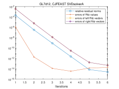
(a) CJ-FEAST SVDsolverA, $d=698,p=21$.

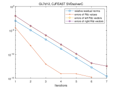
(b) CJ-FEAST SVDsolverC, $d=276,p=21$.

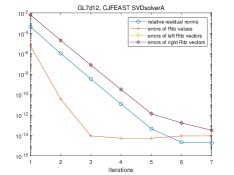
(c) CJ-FEAST SVDsolverA, $d=348,p=26$.

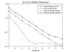
(d) CJ-FEAST SVDsolverC, $d=137,p=26$.

Figure 1: Convergence processes of approximate singular triplets of GL7d12.

For flower_5_4, we take $D=2$ to obtain $d_{a}=928$ and $d_{c}=365$, and take $p=\lceil 1.2\times 137\rceil=165$. The two SVDsolvers converged at iteration steps $k_{a}=8$ and $k_{c}=11$. For rel8, we take $D=2$ to obtain $d_{a}=561$ and $d_{c}=222$, and $p=\lceil 1.1\times 13\rceil=15$. The two SVDsolvers converged at iteration steps $k_{a}=17$ and $k_{c}=20$ separately, roughly the same. In Fig. 2, we depict the convergence processes of the two solvers for computing the singular triplet with $\sigma=4.299030932949072$ of flower_5_4 and $\sigma=13.984665903216351$ of rel8.

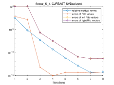
(a) flower_5_4, CJ-FEAST SVDsolverA

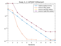
(b) flower_5_4, CJ-FEAST SVDsolverC

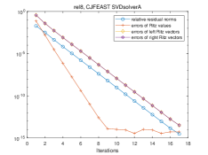
(c) rel8, CJ-FEAST SVDsolverA

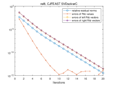
(d) rel8, CJ-FEAST SVDsolverC

Figure 2: Convergence processes of approximate singular triplets for not small singular values.

These experiments justify that the choice strategy (62) of the series degree $d$ works well and, meanwhile, they confirm Remark 7.3. Clearly, we see from Figure 1 and Fig. 2 that the convergence processes of the two solvers are very similar and the Ritz value and the corresponding left and right Ritz vectors have very comparable accuracy at each iteration. These confirm that the CJ-FEAST SVDsolverC and SVDsolverA can compute the singular triplets accurately when the desired singular values are not small but the former more efficient than the latter. We can also find that the errors of Ritz values are approximately squares of those of the left and right Ritz vectors as well as residual norms until the Ritz values have converged with the full accuracy $\|A\|\mathcal{O}(\epsilon_{\mathrm{mach}})$, as the results in Section 2 and Theorem 6.9 indicate.

8.2 Computing singular triplets with small singular values

We apply Algorithm 2 and the CJ-FEAST SVDsolverC to barth5, 3elt_dual and big_dual. For each problem, at least one of the desired singular values is small.

For barth5, one of the desired singular values is $\sigma=1.1050e-8$. We take $D=1$ to obtain $d_{a}=1453$ and $d_{c}=576$, and the subspace dimension $p=\lceil 1.2\times 819\rceil=983$. We run $10$ iterations, and draw their convergence processes in Fig. 3 (a) and (b).

For 3elt_dual, one of the desired singular values is $\sigma=6.8890e-11$. We take $D=1$ to obtain $d_{a}=918$ and $d_{c}=364$, and $p=\lceil 1.1\times 171\rceil=189$. We run $15$ iterations, and draw their convergence processes in Fig. 3 (c) and (d).

For big_dual, one of the desired singular values is $\sigma=8.7726e-13$. We take $D=1$ in (62) to obtain $d_{a}=918$ and $d_{c}=591$, and $p=\lceil 1.2\times 432\rceil=519$. We run $10$ iterations, and draw their convergence processes in Fig. 3 (e) and (f).

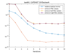
(a) barth5, CJ-FEAST SVDsolverA

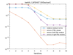
(b) barth5, CJ-FEAST SVDsolverC

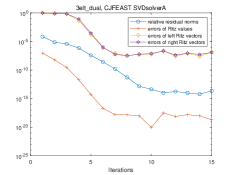
(c) 3elt_dual, CJ-FEAST SVDsolverA

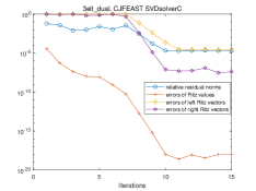
(d) 3elt_dual, CJ-FEAST SVDsolverC

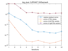
(e) big_dual, CJ-FEAST SVDsolverA

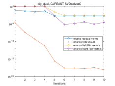
(f) big_dual, CJ-FEAST SVDsolverC

Figure 3: Convergence processes of approximate singular triplets for small singular values.

Several comments are made on Fig. 3. First, for each problem, the left and right Ritz vectors by the CJ-FEAST SVDsolverA always have similar accuracy at the same iteration. Second, the right Ritz vectors computed by the two SVDsolvers have similar accuracy, but the errors of the left Ritz vectors computed by the CJ-FEAST SVDsolverC are a few orders larger than those computed by the CJ-FEAST SVDsolverA. Third, as expected, the relative residual norms of the Ritz approximation by the CJ-FEAST SVDsolverA decrease to $\mathcal{O}(\epsilon_{\mathrm{mach}})$, but those by the CJ-FEAST SVDsolverC stagnate before achieving $\mathcal{O}(\epsilon_{\mathrm{mach}})$ due to the much less accurate left Ritz vectors. In fact, for barth5, 3elt_dual and big_dual, the ultimately relative residual norms are approximately $1e-7,1e-5$ and $1e-3$, respectively, which are precisely $\|A\|/\sigma$ times larger than $\mathcal{O}(\epsilon_{\mathrm{mach}})$. These facts justify our results and analysis in Section 2 and Section 7, and demonstrate that the CJ-FEAST SVDsolverC fails to converge in finite precision arithmetic when (19) is violated. Fourth, the final errors of the Ritz values by the two solvers are $\|A\|\mathcal{O}(\epsilon_{\mathrm{mach}})$, meaning that they compute the singular values $\sigma$ to working precision, independently of the size of $\sigma$.

In summary, the numerical experiments have illustrated that the CJ-FEAST SVDsolverC may not compute left singular vectors as accurately as the right ones and may not make the residual norm drop below a reasonable $tol$ when at least one desired singular value is small. It is conditionally numerically backward stable, but the CJ-FEAST SVDsolverA is always unconditionally numerically backward stable.

9 Conclusions

Based on the convergence results on the CJ-FEAST SVDsolverC, we have made an in-depth analysis of the numerical backward stability of the solver and proved that it may be numerically backward unstable in finite precision arithmetic when computing small singular triplets. The reason is that it may compute the associated left singular vector much less accurately than the right singular vector. Consequently, the residual norms of Ritz approximations may not decrease to a reasonably prescribed tolerance and the solver may thus fail in finite precision arithmetic when $\|A\|/\sigma$ is large.

As an alternative, we have proposed an augmented matrix $S_{A}$ based CJ-FEAST SVDsolverA. It first constructs an approximate spectral projector $P$ of $S_{A}$ associated with all the eigenvalues $\sigma\in[a,b]$ by exploiting the Chebyshev–Jackson series expansion, then performs subspace iteration on $P$ to construct left and right searching subspaces independently, and finally computes the Ritz approximations of the desired singular triplets with respect to the left and right subspaces.

We have derived estimates for the eigenvalues of $P$ and the approximation error $\|P_{S_{A}}-P\|$ in terms of the series degree $d$. We have established convergence results on the approximate left and right singular subspaces and the Ritz approximations, and shown that the left and right Ritz vectors computed by the CJ-FEAST SVDsolverA always have similar accuracy, no matter how small the desired singular values are. We have proved that the ultimate relative residual norms of Ritz approximations can always attain $\mathcal{O}(\epsilon_{\mathrm{mach}})$, meaning that the solver is numerically backward stable in finite precision arithmetic. Therefore, the CJ-FEAST SVDsolverA is more robust than the CJ-FEAST SVDsolverC when $\|A\|/\sigma$ is large. We have made a theoretical comparison of the CJ-FEAST SVDsolverA and SVDsolverC, showing that the latter is at least $2\sqrt[3]{2}$ times as efficient as the former if they both converge for the same tolerance $tol$. Therefore, the CJ-FEAST SVDsolverC and SVDsolverA have their own merits. For the purpose of robustness and overall efficiency, we have proposed a practical choice strategy between the two CJ-FEAST SVDsolvers.

Illuminating numerical experiments have justified all of our results.

Declarations

The two authors declare that they have no financial interests, and they read and approved the final manuscript. The algorithmic Matlab code is available upon reasonable request from the corresponding author.

References

- [1] H. Avron and S. Toledo, Randomized algorithms for estimating the trace of an implicit symmetric positive semi-definite matrix, J. ACM, 58 (2011), pp. Art. 8, 17, https://doi.org/10.1145/1944345.1944349.
- [2] A. Cortinovis and D. Kressner, On randomized trace estimates for indefinite matrices with an application to determinants, Found. Comput. Math., 22 (2022), pp. 875–903, https://doi.org/10.1007/s10208-021-09525-9.
- [3] T. A. Davis and Y. Hu, The University of Florida sparse matrix collection, ACM Trans. Math. Software, 38 (2011), pp. Art. 1, 25, https://doi.org/10.1145/2049662.2049663.
- [4] B. Gavin and E. Polizzi, Krylov eigenvalue strategy using the FEAST algorithm with inexact system solves, Numer. Linear Algebra Appl., 25 (2018), pp. e2188, 20, https://doi.org/10.1002/nla.2188.
- [5] G. H. Golub and C. F. Van Loan, Matrix Computations, Johns Hopkins Studies in the Mathematical Sciences, Johns Hopkins University Press, Baltimore, MD, fourth ed., 2013.
- [6] S. Güttel, E. Polizzi, P. T. P. Tang, and G. Viaud, Zolotarev quadrature rules and load balancing for the FEAST eigensolver, SIAM J. Sci. Comput., 37 (2015), pp. A2100–A2122, https://doi.org/10.1137/140980090.
- [7] J. Huang and Z. Jia, On choices of formulations of computing the generalized singular value decomposition of a large matrix pair, Numer. Algorithms, 87 (2021), pp. 689–718, https://doi.org/10.1007/s11075-020-00984-9.
- [8] T.-M. Huang, Z. Jia, and W.-W. Lin, On the convergence of Ritz pairs and refined Ritz vectors for quadratic eigenvalue problems, BIT, 53 (2013), pp. 941–958, https://doi.org/10.1007/s10543-013-0438-0.
- [9] A. Imakura and T. Sakurai, Complex moment-based method with nonlinear transformation for computing large and sparse interior singular triplets, Sept. 2021, https://doi.org/10.48550/arXiv.2109.13655.
- [10] L. O. Jay, H. Kim, Y. Saad, and J. R. Chelikowsky, Electronic structure calculations for plane-wave codes without diagonalization, Comput. Phys. Commun., 118 (1999), pp. 21–30, https://doi.org/10.1016/S0010-4655(98)00192-1.
- [11] Z. Jia, Using cross-product matrices to compute the SVD, Numer. Algorithms, 42 (2006), pp. 31–61, https://doi.org/10.1007/s11075-006-9022-x.
- [12] Z. Jia and D. Niu, An implicitly restarted refined bidiagonalization Lanczos method for computing a partial singular value decomposition, SIAM J. Matrix Anal. Appl., 25 (2003), pp. 246–265, https://doi.org/10.1137/S0895479802404192.
- [13] Z. Jia and K. Zhang, A FEAST SVDsolver based on Chebyshev–Jackson series for computing partial singular value decompositions of large matrices, 2022, https://doi.org/10.48550/arXiv.2201.02901.
- [14] J. Kestyn, E. Polizzi, and P. T. P. Tang, FEAST eigensolver for non-Hermitian problems, SIAM J. Sci. Comput., 38 (2016), pp. S772–S799, https://doi.org/10.1137/15M1026572.
- [15] J. C. Mason and D. C. Handscomb, Chebyshev Polynomials, Chapman & Hall/CRC, Boca Raton, FL, 2003.
- [16] E. Polizzi, Density-matrix-based algorithm for solving eigenvalue problems, Phys. Rev. B, 79 (2009), pp. e115112, 6, https://doi.org/10.1103/PhysRevB.79.115112.
- [17] E. Polizzi, FEAST eigenvalue solver v4.0 user guide, 2020, https://doi.org/10.48550/arXiv.2002.04807.
- [18] T. J. Rivlin, An Introduction to the Approximation of Functions, Dover Books on Advanced Mathematics, Dover Publications, Inc., New York, 1981.
- [19] Y. Saad, Numerical Methods for Large Eigenvalue Problems, vol. 66 of Classics in Applied Mathematics, SIAM, Philadelphia, PA, 2011, https://doi.org/10.1137/1.9781611970739.
- [20] T. Sakurai and H. Sugiura, A projection method for generalized eigenvalue problems using numerical integration, J. Comput. Appl. Math., 159 (2003), pp. 119–128, https://doi.org/10.1016/S0377-0427(03)00565-X.
- [21] G. W. Stewart, Matrix Algorithms, Vol. II: Eigensystems, SIAM, Philadelphia, PA, 2001, https://doi.org/10.1137/1.9780898718058.
- [22] G. W. Stewart and J. G. Sun, Matrix Perturbation Theory, Computer Science and Scientific Computing, Academic Press, Inc., Boston, MA, 1990.
- [23] P. T. P. Tang and E. Polizzi, FEAST as a subspace iteration eigensolver accelerated by approximate spectral projection, SIAM J. Matrix Anal. Appl., 35 (2014), pp. 354–390, https://doi.org/10.1137/13090866X.