Numerical Investigation of Localization in Two-Dimensional Quasiperiodic Mosaic Lattice

Abstract

A one-dimensional lattice model with mosaic quasiperiodic potential is found to exhibit interesting localization properties, e.g., clear mobility edges [Y. Wang et al., Phys. Rev. Lett. 125, 196604 (2020)]. We generalize this mosaic quasiperiodic model to a two-dimensional version, and numerically investigate its localization properties: the phase diagram from the fractal dimension of the wavefunction, the statistical and scaling properties of the conductance. Compared with disordered systems, our model shares many common features but also exhibits some different characteristics in the same dimensionality and the same universality class. For example, the sharp peak at $g\sim 0$ of the critical distribution and the large $g$ limit of the universal scaling function $\beta$ resemble those behaviors of three-dimensional disordered systems.

I 1. Introduction

Anderson localization of wavefunctions in disordered systems is a subtle consequence of quantum interferenceAderson1958 ; LocalizationReview2 ; LocalizationReview1 ; MarkosReview ; Evers . It is known that electrons in lower dimensions are more prone to localization in the presence of even weak disorderAbrahams79 ; LocalizationReview2 ; LocalizationReview1 ; Evers . Theoretical progressesTheory02 ; Theory03 ; Theory04 ; Theory05 ; Theory06 ; Theory07 and experimental realizationsExperiment01 ; Experiment02 ; Experiment03 ; Experiment04 ; Experiment05 of the delocalization-localization transition (or the metal-insulator transition, MIT) in disordered materials are still exciting topics until today. On the other hand, quasiperiodicity is a delicate structure between order and disorderQuasiCrystalRev1 ; QuasiCrystalRev2 . The most typical case is the Aubry-André-Harper (AAH) model, a one-dimensional (1D) lattice with nearest hopping and with a quasiperiodic potential incommensurate with the underlying lattice structureHarper ; AA . For this 1D model, there exist delocalized states at finite potential magnitude, which is impossible for a completely disordered counterpartAbrahams79 ; MacKinnon . When the quasiperiodic potential magnitude is strong enough, all states will be localized.

Recently the study of quasiperiodic systems has attracted a lot of attentions due to inspiring progresses of experimental realizationsQuasiCrystalRev1 ; QuasiCrystalRev2 ; Experiment2D ; AAHExperiment1 ; AAHExperiment2 ; AAHExperiment3 ; AAHExperiment4 , and its relation with the many body localizationAAHMBL . New analytical methods based on Green’s functions are developed, offering distinct insights into their physical groundsAnalytical01 ; Analytical02 . In the presence of pairing interaction, surprisingly, it was found that the quasiperiodic potential can enhance superconductivity remarkablyEnhancedSC1 ; EnhancedSC2 , suggesting more unexpected phenomena of quasiperiodicity on quantum states. Even in the single particle picture, the quasiperiodic potential results in rich phenomena in different models. Several nontrivial variations of the AAH model have been investigated recently, for instance, generalizations to a dimerized chainRoy or two coupled chainsCoupledChains , with an unbounded quasiperiodic potentialYiCaiZhang2022 or with a relative phase in the quasiperiodic potentialAAH2023 , and higher dimensionsAAModel3D . Novel transport phases and topological phases are found when hoppings are long rangedPowerLawHopping ; LongRangeAAH ; YWang or quasiperiodic as wellOffDiagonalMosaic . Besides these, two-dimensional (2D) quasiperiodic systems provide richer phenomena of localizationMoireLocalization ; Localization2D2020 , topologyShuChen2022 , flat bandFlatBand2022 , and many-body effectsExperiment2D ; ManyBody2022 .

The original 1D AAH model possesses a self duality for the transformation between the real and momentum spaces. This leads to the absence of mobility edges, which means that all eigenstates are either localized or delocalized, depending only on the strength of the potential. Among attempts to break the self duality, a nontrivial modification is the 1D quasiperiodic mosaic lattice, where the quasiperiodic potential only appears at sites with equally spaced distanceWangY . This is an analytically solvable model that exhibits mobility edges separating localized and delocalized states for a fixed potential strength.

In this manuscript, we generalize this quasiperiodic mosaic lattice to a two-dimensional (2D) version on the square lattice and study its localization properties. Different from its 1D counterpart, the phase boundary between localization and delocalization is highly fractal. By varying the initial phase of the quasiperiodic potential, statistical properties of the conductance are studied. In the end, we summarize all numerical results of conductance in a universal scaling function $\beta(g)$, which shows some different features from those in disordered 2D systems. Interestingly, for this 2D quasiperiodic model, some of these properties are similar to those in three-dimensional (3D) disordered systems.

II 2. Model and Methods

Figure 1: Illustration of our 2D quasiperiodic mosaic lattice model with $\kappa=2$. Only solid red sites have nonzero quasiperiodic potential. Each site is represented by its coordinate $(i_{x},i_{y})$ and the nearest hopping is $t$.

Our 2D model is defined on a square lattice with the nearest hopping Hamiltonian

$$\mathcal{H} =\sum_{i_{x},i_{y}}t(c^{\dagger}_{i_{x},i_{y}}c_{i_{x}+1,i_{y}}+c^{\dagger}_{i_{x},i_{y}}c_{i_{x},i_{y}+1})+\mathrm{H.c.}$$ (1)

$$+2\sum_{\bm{i_{x},i_{y}}}V(i_{x},i_{y})c^{\dagger}_{i_{x},i_{y}}c_{i_{x},i_{y}},$$

where $c^{\dagger}_{i_{x},i_{y}}$ ($c_{i_{x},i_{y}}$) creates (annihilate) an electron at the site with integral coordinate $(i_{x},i_{y})$. In the following, the hopping integral $t=1$ will be used as the energy unit, and the lattice constant $a=1$ will be used as the length unit.

The quasiperiodic mosaic potential $V(i_{x},i_{y})$ is a generalization of the 1D version asWangY ; Devakul

$$V(i_{x},i_{y}) =\begin{cases}\lambda F(i_{x},i_{y}),\enspace i_{x}=m\kappa\text{ and }i_{y}=n\kappa,\\ \qquad 0\qquad,\qquad\text{otherwise}\end{cases}$$ (2a)

$$F(i_{x},i_{y}) =\cos\big{[}2\pi(\omega{i_{x}}+\theta_{x})]+\cos[2\pi(\omega{i_{y}}+\theta_{y})\big{]},$$ (2b)

where $\lambda\geqslant 0$ is the amplitude of the potential. The irrational number $\omega$ defines the quasiperiodicity, and the integer $\kappa$ defines the mosaic period as illustrated in Figure 1. When $\kappa=1$ it returns to the original 2D AAH model without mosaic, and only models with $\kappa>1$ can be called mosaic. Recently an endoepitaxial growth of mosaic heterostructures has been experimentally realized on monolayer 2D atomic crystalsMosaic2DExp . In this manuscript, except in Figure 2 (a), we always adopt $\omega=(\sqrt{5}-1)/2$ and $\kappa=2$,WangY . The real numbers $0\leqslant\theta_{x},\theta_{y}<1$ are phase offsets of the potential profile. With other model parameters ($\lambda$, $\omega$ and $\kappa$) fixed, different pairs of $(\theta_{x},\theta_{y})$ corresponds to different realizations of an ensemble, similar to different realizations of a disordered ensembleDevakul . This will be useful when one needs statistical properties of this model, for example, mean values and statistical fluctuations.

Since analytical treatments for a 2D model are more difficult than those in 1D, we will rely on numerical methods, which will be briefly introduced in the following. All of our following calculations are performed in FORTRAN codes, along with Intel Math Kernel Library.

For a square shaped finite sample with $L\times L$ lattice sites, the inverse participation ratio (IPR) of the $m$-th normalized eigenstate $|\Psi_{m,j}\rangle$ is defined asEvers

$$\text{IPR}(L,m)=\sum_{j=1}^{L\times L}|\Psi_{m,j}|^{4}.$$ (3)

Then the localization of the state can be characterized by the fractal dimension of the wavefunction as

$$\mathrm{\Gamma}(L,m)=-\frac{\ln\big{[}\text{IPR}(L,m)\big{]}}{\ln L}.$$ (4)

In the thermodynamic limit $L\to\infty$, the state is extended (localized) if $\lim\limits_{L\to\infty}\Gamma(L)\to 2$ ($\lim\limits_{L\to\infty}\Gamma(L)\to 0$).

The localization properties can also be studied from quantum transports, by attaching two leads to the sample with quasiperiodic potential. At zero temperature, the two-terminal conductance $G_{T}$ at Fermi energy $E$ is proportional to the transmission (Landauer formula)Landauer , and can be expressed asDatta ; Datta2

$$G_{T}(E)=2\frac{e^{2}}{h}g_{T}=2\frac{e^{2}}{h}\mathrm{Tr}\left[\Gamma_{L}(E)G^{r}(E)\Gamma_{R}(E)G^{a}(E)\right],$$ (5)

where the prefactor 2 accounts for the spin degeneracy. Here $G^{r/a}(E)\equiv\left(E\pm-H-\Sigma^{r/a}_{L}-\Sigma^{r/a}_{R}\right)^{-1}$ is the dressed retarded/advanced Green’s function of the central sample, and $\Gamma_{L(R)}=i(\Sigma_{L(R)}^{r}-\Sigma_{L(R)}^{a})$ with $\Sigma_{L(R)}^{r/a}(E)$ being retarded/advanced self energies due to the left (right) lead, respectively. In order to diminish the interface scattering, we take both leads to be lattices identical to the sample with vanishing potential $V$.

Based on the dimensionless conductance $g_{T}$ defined in Equation(5), the appropriate variable for size scaling is the intrinsic conductance $g$ expressed as Braun1997 ; Slevin2001

$$\frac{1}{g}=\frac{1}{g_{T}}-\frac{1}{N_{c}},$$ (6)

with $N_{c}$ the number of active channels at Fermi energy when the potential is absent. The second term $\frac{1}{N_{c}}$ is used to deduct the effect of contact resistance so that the intrinsic transport property of the sample can be manifested. This intrinsic conductance of square shaped ($L\times L$) samples can be used to evaluate the scaling function $\beta=\frac{d\langle\ln g\rangle}{d\ln L}$ of the metal-insulator transition, where $\langle\cdots\rangle$ stands for averaging over an appropriate ensemble Slevin2001 ; LocalizationGraphene ; XRWang2019 . An increase (decrease) of $\ln g$ with increasing $\ln L$ indicates a metal (insulator) phase.

III 3. Results

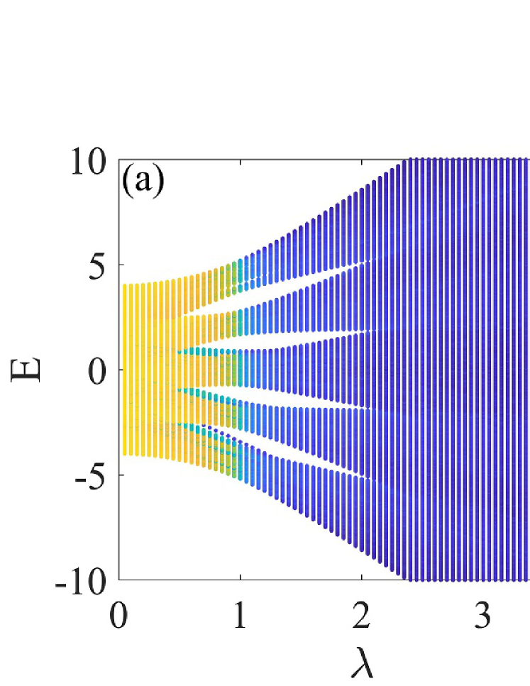
Figure 2: Fractal dimension $\Gamma$ of eigenstates as functions of corresponding eigenvalues $E$ and quasiperiodic potential strength $\lambda$, for a fixed sample size $L=200$. (a) Non-mosaic with $\kappa=1$. (b) Mosaic with $\kappa=2$.

III.1 3.1. Phase diagram from eigenstates

First let us have a global view of the localization property of this model. In Figure 2, we present the fractal dimension $\Gamma$ of eigenstates as functions of potential magnitude $\lambda$ and corresponding eigenenergy $E$, for an isolated $200\times 200$ sample with a definite potential configuration $\theta_{x}=\theta_{y}=0$. For comparison, we present the cases of $\kappa=1$ (non-mosaic) and $\kappa=2$ (mosaic) lattice in panels (a) and (b) respectively. With increasing $\lambda$, the band is broadened outwards and localized states ($\Gamma\sim 0$, blue color) appear. However, there is a remarkable difference between these two cases. For the non-mosaic case [Figure 2 (a)], all states on the energy spectrum transit into localization simultaneously around $\lambda\sim 1$. In other words, there is no mobility edge for this case. For the mosaic case, on the other hand, there are both localized (blue color) and delocalized (orange color) states after $\lambda\gtrsim 0.6$. This distinction between mosaic and non-mosaic models are similar to that in 1D WangY . Also similar to the mosaic lattice in 1DWangY , extended states ($\Gamma\sim 2$, yellow color) mostly distribute around the band center. Although their fraction among all states decreases with increasing $\lambda$, their existence can survive at large $\lambda$. In the following, we will focus on the mosaic lattice only.

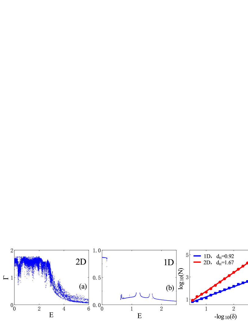
Figure 3: (a) $\Gamma$ as a function of $E$ for $\lambda=2.5$, which is just the cross section shown as the red dotted line in Figure 2 (b). (b) $\Gamma$ as a function of $E$ for a 1D mosaic lattice, with $\lambda=2.5$, $\kappa=2$ and $N_{x}=3000$. (c) The $\log-\log$ plots of box counting parameters $\delta$ versus $N$ for panel (a) (red) and panel (b) (blue), whose slope gives the Hausdorff dimension.

To see more details of this phase diagram in Figure 2 (b) for the 2D mosaic lattice, we plot the profile of $\Gamma(E)$ along the red dashed line at $\lambda=2.5$ in Figure 3 (a). For comparison, a typical counterpart of the 1D model is plotted in Figure 3 (b). Compared to the 1D case, the first obvious feature of the 2D model is strong fluctuations even around adjacent eigenenergies. For example, in the delocalization region $E\lesssim 3$, $\Gamma$ for most eigenstates fluctuate rapidly between $(1.35,1.8)$, and some of them even drop around $\Gamma=1$. Furthermore, the transition between localization and delocalization tends to be a fractal region. In 1D, on the contrary, the profile consists of smooth curves with sudden jumps at transitions. Similar to that shown Figure 3 (a), fractal transitional region of transports is also predicted for the topological transition of a 2D incommensurate bilayer, which is a quasiperiodic structure as wellYuYan2022 .

To characterize the difference between Figure 3 (a) and (b) quantitatively, we calculate the Hausdorff dimension $d_{H}$ of the point set $\big{\{}(\Gamma_{i},E_{i})\big{\}}$ ($i$ is the index of eigenstates) shown in these 2D panels, by using the standard box-counting (BC) method Guarner ; XYang . This algorithm counts the number $N$ of squares with size $\delta$ which are necessary to continuously cover the graph of points $(\Gamma_{i},E_{i})$ rescaled to a unit square. In the intermediate region of $\delta$ (“the scaling region”) where the scaling relation $N\sim\delta^{-d_{H}}$ holds, the slope of the log-log plot of $\delta-N$ is the estimate of the Hausdorff dimension $d_{H}$ Veen ; vanVeen . The results corresponding to Figure 2 (a) and (b) are shown as red and blue plots in panel (c) respectively. As expected, $d_{H}$ for the 1D model is close to $1$, reflecting the fact that $\Gamma(E)$ consists of simple smooth curves. For the 2D model however, $d_{H}\sim 5/3$ suggests that $\Gamma(E)$ is indeed highly fractal. We have checked that (but not shown here) for a very small potential magnitude, say, $\lambda=0.3$, the relative fluctuation of $\Gamma(E)$ of the 2D model can be smaller, but its Hausdorff dimension ($d_{H}=1.68$) is still distinctly larger than that of the 1D model ($d_{H}=0.87$).

III.2 3.2. Transport

The above results were from eigenstates of an isolated sample. Now let us scrutinize transport properties obtained by attaching conducting leads to the sample.

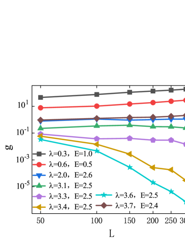
Figure 4: The typical value of the intrinsic conductance $\exp\big{(}\langle\ln g\rangle\big{)}$ as a function of sample size $L$, for different model parameters $\lambda$ and $E$. The sample is square shaped and the average $\langle\cdots\rangle$ is over 150,000 realizations of $(\theta_{x},\theta_{y})$.

The localization (delocalization) can be characterized by the increasing (decreasing) of $g$ [Equation(6)] with growing sample size $L$LocalizationReview1 ; Evers . Similar to the case of disordered systemsSlevin2001 , the conductance should be ensemble averaged before size scaling, to diminish the effect of sharp coherent fluctuations. To this end, we choose $\theta_{x}$ and $\theta_{y}$ to be random variables uniformly distributed within $(0,1)$, and define $\langle\cdots\rangle$ to be the arithmetic average over different realizations of $(\theta_{x},\theta_{y})$. In the following calculations, all averages are over 150,000 realizations. Since $g$ is not a self-averaging quantity and $\ln g$ is “better distributed” than $g$ itself (especially in the case of localization, as will be seen in the following), it is numerically more preferable to extract information from $\langle\ln g\rangle$ (or equivalently the typical value $g^{\text{typ}}\equiv\exp\big{(}\langle\ln g\rangle\big{)}$) rather than the mean value $\langle g\rangle$Slevin2001 ; Evers ; MarkosReview . In Figure 4, we present the typical values of conductance $g^{\text{typ}}$ as functions of the sample size $L$, for different model parameters. There are typical delocalization and localization states with increasing or decreasing $g(L)$ dependence respectively, and also critical states ($\lambda=3.1$ and $E=2.5$) between them.

Besides the averaged quantity, the distribution of the conductance also provides insightful information of localizationEvers ; MarkosReview . In Figs. 5 and 6, we present distributions of $g$ and $\ln g$ respectively, for four typical regimes. In Figure 5 (a) with extremely weak disorder, the conductance has a very small relative deviation $\Delta g/g$. The distribution profile is rather irregular with multiple peaks. This is not surprising because the quasiperiodic potential is not “random-like” enough. Moreover, the energy scale associated with the quasiperiodic potential has not dominated over the level separation of the finite sample yet, so that the transmission can be very sensitive to the competition between these two factors, resulting in multiple peaks of the distribution. With a stronger potential but still in the delocalized state as shown in Figure 5 (b), the distribution is smoothened to be a perfect Gaussian profile. This is identical to what happens in a delocalized state with disorderMarkosReview . From Figure 6 (a) and (b) we can see that in the delocalized regime, the distribution profile of $\ln g$ is almost identical to that of $g$.

At the critical state between localization and delocalization presented in Figure 5 (c), the distribution profile is largely deformed. There is an obvious nonanalytic point at $g=1$, which is also the common feature at the MIT in disordered systemsMarkos2DAndo ; MarkosReview . Another noticeable feature is the sharp peak near $g=0$. From the distribution of $\ln g$ shown in 6 (c) it can be confirmed that this is a peak close to $g=0$, instead of one at $g=0$ Markos2DAndo . Interestingly, such a peak close to $g=0$ is also found at the MIT of a three-dimensional (3D) orthogonal systemMarkosReview , but is absent at that of a 2D symplectic system (the only example to exhibit bulk MIT in 2D)Markos2DAndo ; Marko and at the plateau-plateau transition of a 2D unitary system (quantum Hall effect)Distribution2D ; Evers . In one word, for this 2D quasiperiodic model, the statistical distribution of the MIT exhibits similar behavior to that of a 3D disordered system.

In the localized phase shown in Figure 5 (d), the conductance displays a single-peak distribution highly concentrated around $g=0$, which is also similar to that in the localized phase of disordered systemsDistributionSoukoulis ; DistributionSuslov . In disordered systems with localization, it was found that the quantity $\ln g$ is “better distributed” as a partial Gaussian distribution terminated around $\ln g=0$DistributionSoukoulis ; DistributionSuslov . The distribution of $\ln g$ for our model at strong localization is presented in Figure 6 (d). One can see that, although it is not a typical Gaussian shape but a clear termination around $\ln g$ still persists.

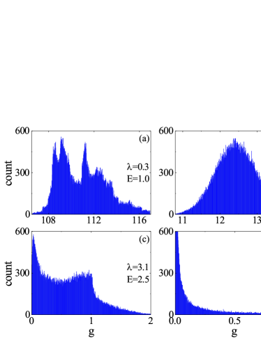
Figure 5: Statistical distribution of $g$ with sample size $L=150$. (a) and (b): the delocalized states with $\beta>0$. (c) The critical state with $\beta=0$. (d) The localized state with $\beta<0$. The statistics is over 150,000 realizations of $(\theta_{x},\theta_{y})$.

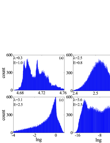
Figure 6: Similar to Figure 5 but for the quantity $\ln g$.

III.3 3.3. Scaling function

For a certain set of model parameters $\{\lambda,\omega\}$, and after a polynomial fitting of data points $(\langle\ln g\rangle,\ln L)$ shown in Figure 4, one can obtain a numerical evaluation of the scaling function $\beta=\frac{d\langle\ln g\rangle}{d\ln L}$. Results of $\beta$ as a function of $\langle\ln g\rangle$ for a wide range of model parameters are shown in Figure 7. Within our best capability of calculation, i.e., 150,000 configurations at size $300\times 300$, there are still strong fluctuations, especially around the transition region, $\beta\sim 0$, which is consistent with what we have seen from Figure 3 (a) and Figure 5 (c). Nevertheless, some useful information can still be drawn. Firstly, all data points, similar to the case of disordered systemsSlevin2001 , tend to collapse around a universal curve. We manage to fit these data with an appropriate nonlinear function. Numerically, among common functions we find that the Boltzmann function provides the best smooth curve that fits these data with the expression

$$\beta(\ln g) = A_{1}+\frac{\displaystyle A_{1}-A_{2}}{\displaystyle 1+\exp\big{[}(\ln g-x_{0})/\Delta\big{]}},$$ (7)

$$A_{1} = -9.387,\qquad A_{2}=0.755,$$

$$x_{0} = -5.038,\qquad\Delta=1.550$$

which is plotted as the blue dashed curve. This is a monotonic function with a single zero point at $\ln g_{c}=-1.130$ where the MIT occurs. We stress again that this Boltzmann function is just an empirical choice instead of a principle-based analytical result, and we merely use it to extract some useful quantities in a numerically convenient way. For example, the slope of $\beta\big{(}\ln g\big{)}$ at its zero gives the inverse of $\nu$, the critical exponent characterizing the the divergence of the localization (correlation) length near the critical pointLocalizationReview1 ; Slevin2001 . From Equation(III.3) we have an estimate $\nu\sim 2.22$. This value is larger than those of MITs in 3D, and that of MIT in 2D symplectic systemsSlevin2001 ; DNShengCriticalExponents , but is close to that of the plateau-plateau transition of 2D quantum Hall effects (unitary system)QHEnu1 ; QHEnu2 ; QHEnu3 ; QHEnu4 . Another important feature is the saturation of $\beta\sim 1$ at large $\ln g$ limit. For disordered systems, it has been known that the $\epsilon$ expansion in the large conductance limit gives $\beta\rightarrow D-2$, for all three universality classesEpsilonExpansion1 ; EpsilonExpansion2 ; LocalizationReview2 ; Slevin2017 . In this sense, the scaling behavior of our 2D quasiperiodic model in the weak potential (therefore large conductance) limit seems to resemble that of the 3D disordered model.

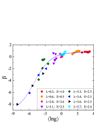
Figure 7: The scaling function $\beta(g)=d\langle\ln g\rangle/d\ln L$ as a function of $\langle\ln g\rangle$ in the two-dimensional quasiperiodic mosaic lattice. Dots are numerical differential (see text) results from data shown in Figure 4. The dashed curve is a numerical fitting of these dots with the expression Equation(III.3).

IV 4. Summary and Discussion

In this paper, we numerically investigate the localization properties of the 2D quasiperiodic mosaic lattice model. We find some properties similar to, and also some different from those of 2D disordered systems.

Similar to the 1D counterpart, there exists localization-delocalization transition when varying the energy and the strength of the quasiperiodic potential. However the transition region is fractal like, contrary to clear phase boundaries in 1D. This model shares many common statistical features of the conductance $g$, for example, Gaussian-like distribution in the delocalized phase, high peak near zero in the localized phase, and the existence of non-analytical behavior of the distribution function at the critical point between two phases. However, this critical distribution at the small $g$ limit shows a sharp peak around zero, which is a particular feature of the 3D disordered systems. The scaling function $\beta$ is also a universal function of $g$, but its large $g$ limit approaches 1, which is also the feature of 3D disordered systems. This may suggest a novel role of the spatial dimensionality of quasiperiodic systems, which will be studied in the future. QuasiCrystalRev1 ; QuasiCrystalRev2 .

V Acknowledgements

This work was supported by National Natural Science Foundation of China under Grant Nos. 12104108, 11774336 and 11874127, the Joint Fund with Guangzhou Municipality under Nos. 202201020198 and 202201020137, and the Starting Research Fund from Guangzhou University under Grant Nos. RQ2020082, RQ 2020083 and 62104360.

References

- (1) Anderson P W 1958 Phys. Rev. 109 1492
- (2) Lee P A and Ramakrishnan T V 1985 Rev. Mod. Phys. 57 287
- (3) Kramer B and MacKinnon A 1993 Rep. Prog. Phys. 56 1469
- (4) Markoš P 2006 Acta Phys. Slov. 56 561
- (5) Evers F and Mirlin A D 2008 Rev. Mod. Phys. 80 1355
- (6) Abrahams E, Anderson P W, Licciardello D C and Ramakrishnan T V 1979 Phys. Rev. Lett. 42 673
- (7) Corona-Patricio G, Kuhl U, Mortessagne F, Vignolo P and Tessieri L 2019 New J. Phys. 21 073041
- (8) Lemarié G 2019 Phys. Rev. Lett. 122 030401
- (9) Werner M A, Brataas A, von Oppen F and Zaránd G 2019 Phys. Rev. Lett. 122 106601
- (10) Souza A M C, Almeida G M A and Mucciolo E R 2020 J. Phys.: Condens. Matter 32 285504
- (11) Ohtsuki T and Mano T 2020 J. Phys. Soc. Jpn. 89 022001
- (12) Horváth I and Markoš P 2022 Phys. Rev. Lett. 129 106601
- (13) Lopez M, Clément J-F, Szriftgiser P, Garreau J C and Delande D 2012 Phys. Rev. Lett. 108 095701
- (14) Signoles A, Lecoutre B, Richard J, Lim L-K, Denechaud V, Volchkov V V, Angelopoulou V, Jendrzejewski F, Aspect A, Sanchez-Palencia L and Josse V 2019 New J. Phys. 21 105002
- (15) Rehemanjiang A, Richter M, Kuhl U and Stöckmann H-J 2020 Phys. Rev. Lett. 124 116801
- (16) Jäck B, Zinser F, König E J, Wissing S N P, Schmidt A B, Donath M, Kern K and Ast C R 2021 Phys. Rev. Res. 3 013022
- (17) Sajjad R, Tanlimco J L, Mas H, Cao A, Nolasco-Martinez E, Simmons E Q, Santos F L N, Vignolo P, Macrì T and Weld D M 2022 Phys. Rev. X 12 011035
- (18) Jagannathan A 2021 Rev. Mod. Phys. 93 045001
- (19) Fan J and Huang H 2022 Front. Phys. 17 13203
- (20) Harper P G 1955 Proc. R. Soc. London, Ser. A. 68 874
- (21) Aubry S and André G 1980 Ann. Israel Phys. Soc. 3 133
- (22) MacKinnon A and Kramer B 1981 Phys. Rev. Lett. 47 1546
- (23) Bordia P, Lüschen H, Scherg S, Gopalakrishnan S, Knap M, Schneider U, and Bloch I 2017 Phys. Rev. X 7 041047
- (24) Lüschen H P, Scherg S, Kohlert T, Schreiber M, Bordia P, Li X, Sarma S D and Bloch I 2018 Phys. Rev. Lett. 120 160404
- (25) An F A, Meier E J and Gadway B 2018 Phys. Rev. X 8 031045
- (26) Kohlert T, Scherg S, Li X, Lüschen H P, Sarma S D, Bloch I and Aidelsburger M 2019 Phys. Rev. Lett. 122 170403
- (27) An F A, Padavić K, Meier E J, Hegde S, Ganeshan S, Pixley J H, Vishveshwara S and Gadway B 2021 Phys. Rev. Lett. 126 040603
- (28) Zhang S-X and Yao H 2018 Phys. Rev. Lett. 121 206601
- (29) Duthie A, Roy S and Logan D E 2021 Phys. Rev. B 103 L060201
- (30) Duthie A, Roy S and Logan D E 2021 Phys. Rev. B 104 064201
- (31) Fan Z, Chern G-W and Lin S-Z 2021 Phys. Rev. Res. 3 023195
- (32) Zhang X and Foster M S 2022 Phys. Rev. B 106 L180503
- (33) Roy S, Mishra T, Tanatar B and Basu S 2021 Phys. Rev. Lett. 126 106803
- (34) Rossignolo M and Dell’Anna L 2019 Phys. Rev. B 99 054211
- (35) Zhang Y C and Zhang Y Y 2022 Phys. Rev. B 105 174206
- (36) Cai X and Yu Y-C 2023 J. Phys.: Condens. Matter 35 035602
- (37) Devakul T and Huse D A 2017 Phys. Rev. B 96 214201
- (38) Deng X, Ray S, Sinha S, Shlyapnikov G V and Santos L 2019 Phys. Rev. Lett. 123 025301
- (39) Roy N and Sharma A 2021 Phys. Rev. B 103 075124
- (40) Wang Y, Xia X, Wang Y, Zheng Z and Liu X-J 2021 Phys. Rev. B 103 174205
- (41) Zeng Q-B and Lü R 2021 Phys. Rev. B 104 064203
- (42) Huang B and Liu W V 2019 Phys. Rev. B 100 144202
- (43) Szabó A and Schneider U 2020 Phys. Rev. B 101 014205
- (44) Xu Z-H, Xia X, and Chen S Chen 2022 Sci. China- Phys. Mech. Astron. 65 227211
- (45) Wang Y Wang, Zhang L,Wan Y, He Y, and Wang Y 2022 arXiv:2209.14741
- (46) Štrkalj A, Doggen E V H, and Castelnovo C 2022 Phys. Rev. B 106 184209
- (47) Wang Y, Xia X, Zhang L, Yao H, Chen S, You J, Zhou Q and Liu X-J 2020 Phys. Rev. Lett. 125 196604
- (48) Devakul T and Huse D A 2017 Phys. Rev. B 96 214201
- (49) Zhang Z, Huang Z, Li J, Wang D, Lin Y, Yang X, Liu H, Liu S, Wang Y, Li B, Duan X and Duan X 2022 Nat. Nanotechnol. 17 493
- (50) Imry Y and Landauer R 1999 Rev. Mod. Phys. 71 S306
- (51) Datta S 1995 Electronic Transport in Mesoscopic Systems (Cambridge: Canmbridge University Press)
- (52) Datta S 2005 Quantum Transport: Atom to Transistor (Cambridge: Canmbridge University Press)
- (53) Braun D, Hofstetter E, Montambaux G and MacKinnon A 1997 Phys. Rev. B 55 7557
- (54) Slevin K, Markoš P and Ohtsuki T 2001 Phys. Rev. Lett. 86 3594
- (55) Bang J and Chang K J 2010 Phys. Rev. B 81 193412
- (56) Chen W, Wang C, Shi Q, Li Q and Wang X R 2019 Phys. Rev. B 100 214201
- (57) Yu Y, Zhang Y-Y, Wang S-S, Guan J-H, Yang X, Xia Y and Li S-S 2022 New J. Phys. 24 083029
- (58) Guarneri I and Terraneo M 2001 Phys. Rev. E 65 015203(R)
- (59) Yang X, Zhou W, Zhao P and Yuan S 2020 Phys. Rev. B 102 245425
- (60) van Veen E, Tomadin A, Polini M, Katsnelson M I and Yuan S 2017 Phys. Rev. B 96 235438
- (61) van Veen E, Yuan S, Katsnelson M I, Polini M and Tomadin A 2016 Phys. Rev. B 93 115428
- (62) Markoš P and Schweitzer L 2006 J. Phys. A: Math. Gen. 39 3221
- (63) Markoš P and Schweitzer L 2006 J. Phys. A 39 3221
- (64) Ohtsuki T, Slevin K and Kramer B 2004 Physica E 22 248
- (65) Suslov I M 2017 J. Exp. Theor. Phys. 124 763
- (66) Rühländer M and Soukoulis C M 2001 Phys. B: Condens. Matter 296 32
- (67) Sheng D N and Weng Z Y 1999 Phys. Rev. Lett. 83 144
- (68) Mil’nikov G and Sokolov I 1988 JETP Lett. 48 536
- (69) Chalker J T and Coddington P D 1988 J. Phys. C 21 2665
- (70) Huckestein B and Kramer B 1990 Phys. Rev. Lett. 64 1437
- (71) Slevin K and Ohtsuki T 2009 Phys. Rev. B 80 041304(R)
- (72) Wegner F 1989 Nucl. Phys. B 316 663
- (73) Hikami S 1992 Prog. Theor. Phys. Suppl. 107 213
- (74) Ueoka Y and Slevin K 2017 J. Phys. Soc. Jpn. 86 094707