Improving Reliability of Fine-tuning with Block-wise Optimisation

Abstract

Finetuning can be used to tackle domain-specific tasks by transferring knowledge learned from pre-trained models. However, previous studies on finetuning focused on adapting only the weights of a task-specific classifier or re-optimising all layers of the pre-trained model using the new task data. The first type of methods cannot mitigate the mismatch between a pre-trained model and the new task data, and the second type of methods easily cause over-fitting when processing tasks with limited data. To explore the effectiveness of fine-tuning, we propose a novel block-wise optimisation mechanism, which adapts the weights of a group of layers of a pre-trained model. In our work, the layer selection can be done in four different ways. The first is layer-wise adaptation, which aims to search for the most salient single layer according to the classification performance. The second way is based on the first one, jointly adapting a small number of top-ranked layers instead of using an individual layer. The third is block based segmentation, where the layers of a deep network is segmented into blocks by non-weighting layers, such as the MaxPooling layer and Activation layer. The last one is to use a fixed-length sliding window to group layers block by block. To identify which group of layers is the most suitable for finetuning, the search starts from the target end and is conducted by freezing other layers excluding the selected layers and the classification layers. The most salient group of layers is determined in terms of classification performance. In our experiments, the proposed approaches are tested on an often-used dataset, $Tf\_flower$, by finetuning five typical pre-trained models, VGG16, MobileNet-v1, MobileNet-v2, MobileNet-v3, and ResNet50v2, respectively. The obtained results show that the use of our proposed block-wise approaches can achieve better performances than the two baseline methods and the layer-wise method.

I Introduction

The rapid development of deep learning technologies has made it easy to construct and train complex neural networks [1]. The deep structure of neural networks has thus gained tremendous success. However one of their critical challenges is that it needs large amounts of data. Training a model for a specific task on a limited data can lead to poor generalization due to over-fitting. Although lots of data can be now collected online, data annotation is always an expensive and time-consuming task. Therefore, more often in practice, one would fine-tune existing networks by continuing training it on the new task data. This can benefit many applications not having sufficient data by transferring learned knowledge from multiple sources to a domain-specific task [2, 3].

Fine-tuning can process a pre-trained network in three different ways. The first is to freeze all the weights of the pre-trained network, but optimise only classifier layers using new task data. The second is to optimise the weights of all layers. The last one is done by adapting the weights of a subset layers of the pre-trained model as they would be more useful to learn dataset-specific features than other layers.

In our preliminary experiments, we noticed that randomly tuning few individual layers of a pre-trained deep network can yield different performances, and occasionally outperform the first two fine-tuning methods mentioned above. We thus hypothesised that fine-tuning a group of layers may lead to some interesting results. Although fine-tuning a subset of layers seems to be more instinctively reasonable than the first two, it is not yet fully investigated how to determine which layers in the pre-trained network can have a greater contribution than other layers, when being tuned on new task data. We therefore propose a novel framework using block-wise fine-tuning in this paper and aim to explore an efficient way to find out the salient layers relevant to the features of new task data and improve fine-tuning reliability.

The block-wise mechanism is conducted by dividing a deep network into blocks, each of which consists of a group of layers. To find out the most salient block to the target of a new task, the block-wise fine-tuning can be implemented in four different ways in our work. The first way is layer-wise fine-tuning, which aims to search for the most salient individual layer according to the obtained accuracy on target data. The second way is based on the results of layer-wise adaptation. It aims to jointly fine-tune the weights of several top-ranked layers instead of using only an individual layer since multiple layers could benefit fine-tuning as more parameters are to be adapted. The third way is block wise fine-tuning, where the layers of a deep network are segmented into blocks by non-weighting layers, such as the MaxPooling layer and Activation layer. The last one is to use a fixed-length sliding window to group layers block by block. The most salient block is identified in terms of the accuracy performance obtained by fine-tuning a subset layers. The details of our proposed approaches will be introduced in the next sections.

The rest of this paper is organised as follows: Section 2 introduces the previous studies in relation to fine-tuning; the theoretical framework is presented in detail in Section 3; Section 4 and 5 describe the data set used in this work and experimental set-up; The results and analysis of our experiments are presented in Section 6, and finally conclusions are drawn in the last section.

II Related Work

Within the framework of transfer learning and relying on the architecture of a pre-trained model (PTM), fine-tuning can adapt the model parameters on the target data and has become one of the most promising deep learning techniques in different research fields, such as computer vision (CV), natural language processing (NLP), and speech processing.

II-A Fine-tuning in Computer vision

In computer vision community, the annual ImageNet Large Scale Visual Recognition Challenge (ILSVRC) [4] provided multiple images sources and has resulted in a number of innovations in the architecture, such as VGG[5], Inception[6, 7], MobileNetV2[8], and ResNet50[9]. By fine-tuning, these high-performing pre-trained models are now widely used in image generation[10, 13], image classification[14, 15, 16, 17], image caption[11, 12], anomaly detection[18, 19, 20], image retrieval [21, 22], etc. In these previous studies, the development of fine-tuning techniques in CV can be found.

The first aspect of fine-tuning is layer wise adaptation. Regarding the studies on the roles of hidden layers, Yosinski et al. [27] conducted empirical study to quantify the degree of generality and specificity of each layer in deep networks. The related studies [27, 28] further claimed that the low-level layers extract general features and the high-level layers extract task-specific features in a deep network. Since then, further works have been conducted to exploits the role of each layer. In [29], Tajbakhsh et al. showed that tuning only a few high-level layers is more effective than tuning all layers. Guo et al. [30] proposed an auxiliary policy network that decides whether to use the pre-trained weights or fine-tune them in layer-wise manner for each instance. In [17], Ro et al. proposed an algorithm that improves fine-tuning performance and reduces network complexity through layer-wise pruning and auto-tuning of layer-wise learning rates. To further reinforce auto-tuning of layer-wise learning rate, Tanvir et al. [31] proposed RL-Tune, a layer-wise fine-tuning framework for transfer learning which leverages reinforcement learning (RL) to adjust learning rates as a function of the target data shift.

The second aspect of fine-tuning is in relation to hyper-parameter optimisation. This is because the increasing complexity of deep learning architectures slow training partly caused by “vanishing gradients”. In which the gradients used by back-propagation are extremely large for weights connecting deep layers (layers near the output layer), and extremely small for shallow layers (near the input layer); this results in slow learning in the shallow layers[32]. So, Bharat et al. [32] proposed a method to allow larger learning rates to compensate for the small size of gradients in shallow layers. Since then, various approaches have been explored for better regularization of the transfer learning with effective hyper-parameter selection. In [33] Kornblith et al. proposed a grid-search based approach to search for better hyper-parameters, and Li et al. [3] provided an elaborate guideline of learning rates and other hyper-parameter selections. Furthermore, Parker et al. proposed provably efficient online hyperparameter optimization with population-based bandits, which is found to be effective in optimizing RL training [34] . To improve fine-tuning by using optimiser, Loshchilov et al. [39] designed two robust optimisers, SGDW and AdamW, by combining SGD [35] and Adam [36] with decoupled weight decay. The work in [37, 38] also explored the use of two optimisers, SGD and AdamW, on ImageNet like domains in terms of fine-tuning accuracy. Recently, [40] found that large gaps in performance between SGD and AdamW occur when the fine-tuning gradients in the first “embedding” layer are much larger than in the rest of the model, and claimed that freezing only the embedding layer can lead to SGD performing competitively with AdamW while using less memory.

The third aspect is neural architecture search (NAS), aiming to adapt the architecture of a pre-trained network to match to the characteristics of new task data. Liu et al. [23] used a sequential model-based optimization to guide the search through the architecture of the network. Pham et al. [24] proposed an efficient NAS (ENAS) with parameter sharing, which focuses on reducing the computational cost of NAS by reusing the trained weights of candidate architectures in subsequent evaluations. Lu et al. [25] proposed neural architecture transfer (NAT) to efficiently generate task-specific custom NNs across multiple objectives. Kim et al. [26] proposed to reduces the search cost using given architectural information and cuts NAS costs by early stopping to terminate the search process in advance. In [15], Tanveer et al. developed differentiable neural architecture search method by introducing a differentiable and continuous search space instead of a discrete search space and achieves remarkable efficiency, incurring a low search cost.

II-B Fine-tuning in Natural Language Processing

Compared to CV, NLP models was typically more shallow and thus require different fine-tuning methods [41]. In NLP, Mikolov et al. [42] proposed a simple transfer technique by fine-tuning pre-trained word embeddings, a model’s first layer, but has had a large impact in practice and is now used in most state-of-the-art models. To mitigate LMs’ overfitting to small datasets, Jeremy et al. [41] proposed discriminative language model fine-tuning to retain previous knowledge and avoid catastrophic forgetting. In the last couple of years, large language models, such as GPT [43] and BLOOM [44], were developed by using mask learning on large amounts of text data. Given the size of these large language models, fine-tuning all the model parameters can be compute and memory intensive [45]. Some recent studies [46, 47] have proposed new parameter efficient fine-tuning methods that update only a subset of the model’s parameters. As adversarial samples of new task are usually out-of-distribution, adversarial fine-tuning fails to memorize all the robust and generic linguistic features already learned during pre-training. To mitigate the impacts caused by this, Dong [48] et al. proposed to use mutual information to measure how well an objective model memorizes the useful features captured before. Furthermore, Mireshghallah et al. [49] empirically studied memorization of fine-tuning methods using membership inference and extraction attacks as large models have a high capacity for memorizing training samples during pre-training.

II-C Fine-tuning in Speech Processing

For speech processing, fine-tuning can work not only for language model adaptation [50, 53], but also for tuning acoustic models [51, 52, 54, 55]. Fine-tuning language models in speech processing is same as its use in NLP. Guillaume et al. [53] developed a method using a transformer architecture to tune a generic pre-trained representation model for phonemic recognition. For acoustic model adaptation, Violeta et al. [51] proposed an intermediate fine-tuning step that uses imperfect synthetic speech to close the domain shift gap between the pre-training and target data. Tsiamas et al. [52] proposed to use an efficient fine-tuning technique that trains only specific layers of our system, and explore the use of adapter modules for the non-trainable layers. Peng et al. [55] used fine-tuning to learn robust acoustic representation to alleviate the mismatch between a pre-trained model and new task data. The similar work can be also found in [56], where Haidar et al. employed Generative Adversarial Network (GAN) [57] to fine-tune a pre-trained model to match to the acoustic characteristics of new task data.

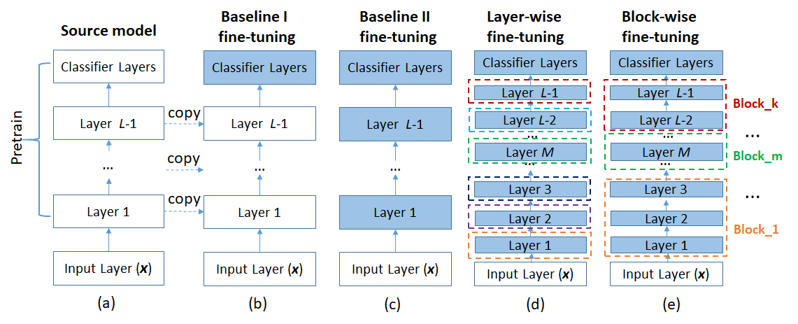
Figure 1: Architectures of source model and four target models: (a) source model (b) fine-tuning only classifier layers of source model , (c)fine-tuning all layers of source model, (d)target model adapted by layer-wise fine-tuning, and (e) target model adapted by block-wise fine-tuning.

III Theoretical Framework

Fine-tuning (FT) in this work is to adapt the weights (W) of a group of layers (Ls) of a pre-trained deep neural network (DN) given input data matrices $\textbf{X}=\{X_{1},X_{2},\ldots,X_{M}\}$ , where $M$ is the number of training samples of a new task, and $X_{m}$ represents the $m$-th sample matrix. The aim of the proposed approach is to find out the block $\textbf{B}_{Ls}$ most relevant to the target data. This can be represented by:

$$\textbf{B}_{Ls,W}=\arg\max_{\textbf{Ls,W}}Accuray(\textbf{DN}(\textbf{X}))$$ (1)

To attain the aim, we designed block-wise fine-tuning alongside the work on layer-wise fine-tuning. Fig. 1 shows the architectures of source model and four target models for fine-tuning. Fig. 1(a) is the pre-trained source model. Fig. 1(b) shows the target model (Baseline I) where only classifier layers marked blue are to be adapted and the weights of other layers will be freezed. Fig. 1(c) is the target model (Baseline II), where all layers are to be re-optimised. The two target models will be used as baseline models for a comparison in this paper. Fig. 1(c) and (d) show the architectures of layer-wise and block-wise fine-tuning, respectively. The dash box means when a layer or a group layers are being tuned, the weights of other layers, except classifier layers, keep fixed.

III-A Layer-wise Fine-tuning

As aforementioned in the first two sections, domain shift between the pre-trained model and target data is the main reason why fine-tuning is needed. The shift is actually accumulated by each individual layer of the pre-trained model. So, our study in fine-tuning starts from layer-wise adaptation. As shown in Fig. 1(d), the weights of each layer will be adapted to search for the layer, which can result in a salient improvement after its weights are adapted on new task data. The pseudo code in Algorithm 1 shows the implementation of layer-wise fine-tuning, where a while loop is used to search for the salient layer. In our approach, the use of a small part of data, e.g. $10\%$, is to identify the most salient layer and thus improve the fine-tuning efficiency.

Algorithm 1 Layer-wise fine-tuning (FT)

1:Load the weights, W, of a pre-trained model (DN)

2:Preprocess input data, X, and select 10% data for training and 30% data for evaluation

3:$N=$ # layers of DN

4:Initialise layer index, $i=1$,

5:Initialise accuracy array, $Acc=zeros(N)$

6:Training:

7:  While $i<N$

8:      tune the weights of the $i^{th}$ layer, $L_{i}$, and classifier

9:      $Acc[i]=\textbf{FT}(\textbf{\text{DN}}(L_{i},C))$

10:      $i=i+1$

11:  EndWhile

12:  Identify the most salient layer, $L_{opt}$, using $Acc$

13:Evaluation:

14:  Fine-tune the layer, $L_{opt}$, of the pre-trained model using all training data $(70\%)$

15:  Evaluate the tuned model on the test data

III-B Block-wise Fine-tuning

In a deep neural network, several adjacent layers with a similar function can be often grouped into a block. Tuning the weights of these layers in a block rather than all layers is an efficient way to match the learned knowledge to a specific task since only a relatively small part of parameters will be adapted. Fig. 1(d) shows the architecture of block-wise fine-tuning, starting from the input end of a deep network.

For block-wise fine-tuning, its critical step is to divide the structure of a deep neural network into blocks. In our work, the division can be done by non-weighting layers, such as the Maxpooling layer and Activation layer. In some typical deep neural networks, such as VGG16[5] and ResNet50[9], there include not only Convolutional layers, but also MaxPooling, Batch Normalization, and Activation layers. The convolutional layers in these models generally contain major parameters, and only a relatively small number of parameters are from other layers. This means Maxpooling layer, Batch Normalization layer, and even Activation layers could be viewed as a delimiter to segment a deep neural network into blocks.

Fig. 2 shows the number of parameters of each layer of VGG16, a classical deep neural network for image classification. In this figure, MaxPooling layers are corresponding to the valleys of the curve since they are non-weighting layers.

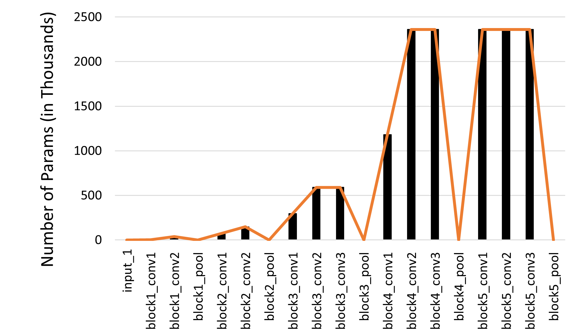
Figure 2: Distribution of the number of parameters of each layer of VGG16 model.

Algorithm 2 Block-wise fine-tuning (FT)

1:Load the weights, W, of a pre-trained model (DN)

2:Preprocess input data, X, and select 10% data for training and 30% data for evaluation

3:$N=$ # Blocks of DN

4:Initialise layer index, $i=1$,

5:Initialise accuracy array, $Acc=zeros(N)$

6:Training:

7:  While $i<N$

8:      tune the weights of the layers in the $i^{th}$ block, $B_{i}$,

9:      and classifier

10:      $Acc[i]=\textbf{FT}(\textbf{\text{DN}}(B_{i},C))$

11:      $i=i+1$

12:  EndWhile

13:  Identify the most salient block, $B_{opt}$, using $Acc$

14:Evaluation:

15:  Fine-tune $B_{opt}$ of the pre-trained model using all training data (70%)

16:  Evaluate the tuned model on the test data

Algorithm 2 shows the pseudo code of implementing block-wise fine-tuning, where a while loop is run over blocks instead of individual layers used in Algorithm 1. As an alternative, we can also use a sliding window instead of non-weight layers to segment the long layer sequence into block. The difference is that the length of the sliding window is fixed and the number of layers in each block will thus be the same. The window length is set to be three in our experiments.

III-C Block-wise Fine-tuning using ranked layers

Unlike Algorithm 2 to segment layers into blocks, another block-wise fine-tuning approach is to select multiple layers, whose contributions to target performance are top-ranked. We thus make use of the evaluation performance on each individual layer obtained by using Algorithm 1. In our experiments, we select top three layers to make up a block.

Algorithm 3 Block-wise fine-tuning using ranked layers

1:Load the weights, W, of a pre-trained model (DN)

2:Preprocess input data, X, to match to the input layer of DN

3:$N=$ # layers of DN

4:Initialise layer index, $ii=0$

5:  Initialise accuracy array, $Acc=zeros(N)$

6:Training:

7:   Implement Algorithm 1

8:   Identify three top-ranked layers in terms of $Acc$

9:Evaluation:

10:  fine-tune the selected three layers of pre-trained model using all training data $(70\%)$

11:  test the tuned model on the test data

IV Data set

The algorithms were tested on the Tf_flowers dataset [58]. The Tf_flowers dataset is a collection of images of flowers, divided into five different classes: daisy, dandelion, roses, sunflowers, and tulips. There are a total of 3670 images in the dataset. The images are high quality color images resized to a resolution of $224\times 224$ pixels, then we scaled RGB to 0-1 range. The dataset is intended for use in image classification tasks, and can be used to train machine learning models to recognize different types of flowers [59].

V Experimental set-up

The training process for this experiment involves using the pre-trained models as a starting point, and then fine-tuning the models on the TensorFlow Flowers dataset. We used TensorFlow Keras library to build and train the models. The training process will involve using a small number of training samples, i.e., 10% of the dataset, to identify the best performing layers (for Layer-wise FT), block (for Block-wise FT ), or Ranked block (for Block-wise with ranked layers FT). Then using the remaining training dataset (70% of the whole dataset) to evaluate the accuracy.

We have evaluated the performance of the algorithms on five commonly used pre-trained models, i.e., VGG16 [5], MobileNet [60], MobileNetV2 [8], MobileNetV3 [61], and ResNet50 [9]. The models were pre-trained on the imagenet wights.

The classifier layers, we started with a Flatting layer [63], to which flattens the dimensions of the output to prepare it for use in Fully Connected (FC) layers [65]. Then a dense layers [64], with 128 units, followed by a dropout layer [62] with a rate of 0.5, to reduce the probability of overfitting. [67]. Then two dense layers with 64 and 5 units respectively. The 64 units layer is activated by a ‘relu’ function, and the final dense layer has five units, activated by ‘softmax’ for the multi-class classification [66].

The model is then compiled with loss function “categorical cross-entropy”, an optimizer “Adam” with a learning rate of $5\times 10^{-5}$ and metrics as “accuracy”. A “Reduce LR On Plateau” callback is then defined, which reduces the learning rate when the validation accuracy plateaus. [65]. The model is then trained on the training data with batch size of 4, 50 epochs and validation data and callbacks.

VI Results and Analysis

In this paper, we began our investigation by evaluating the performance of a Baseline I model, which only tunes the classifier layers, a Baseline II model, which tunes all layers, and a model that randomly tunes three layers using only 10% of the dataset for training. As shown in Fig. 3, the model with randomly chosen layers outperforms the Baseline I method in all tested models, and achieves a comparable performance with Baseline II.

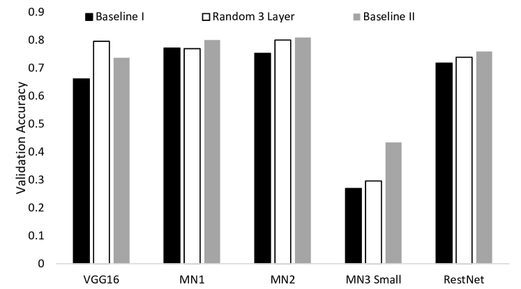
Figure 3: Comparison between the baseline models and FT three randomly selected layers using 10% of the dataset.

Afterwards we investigated the performance of the layer-wise FT approach. As shown in Fig. 4, the classifier accuracy varies significantly between different layers. A very few layer are able to identify the classes with a high accuracy, even exciting both Baseline approaches, while the vast majority would not achieve high accuracy.

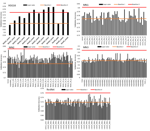
Figure 4: Layer-wise fine tuning accuracy using 10% of the dataset for all tested models.

For the block-wise FT, we implemented it using the pre-trained models with the 10% of the dataset. The results shown in Fig. 5. We can observe that the classification accuracy has been significantly improved with the use of block wise FT, and the accuracy has a certain observable pattern. We can also note that the highest accuracy blocks are not usually convective.

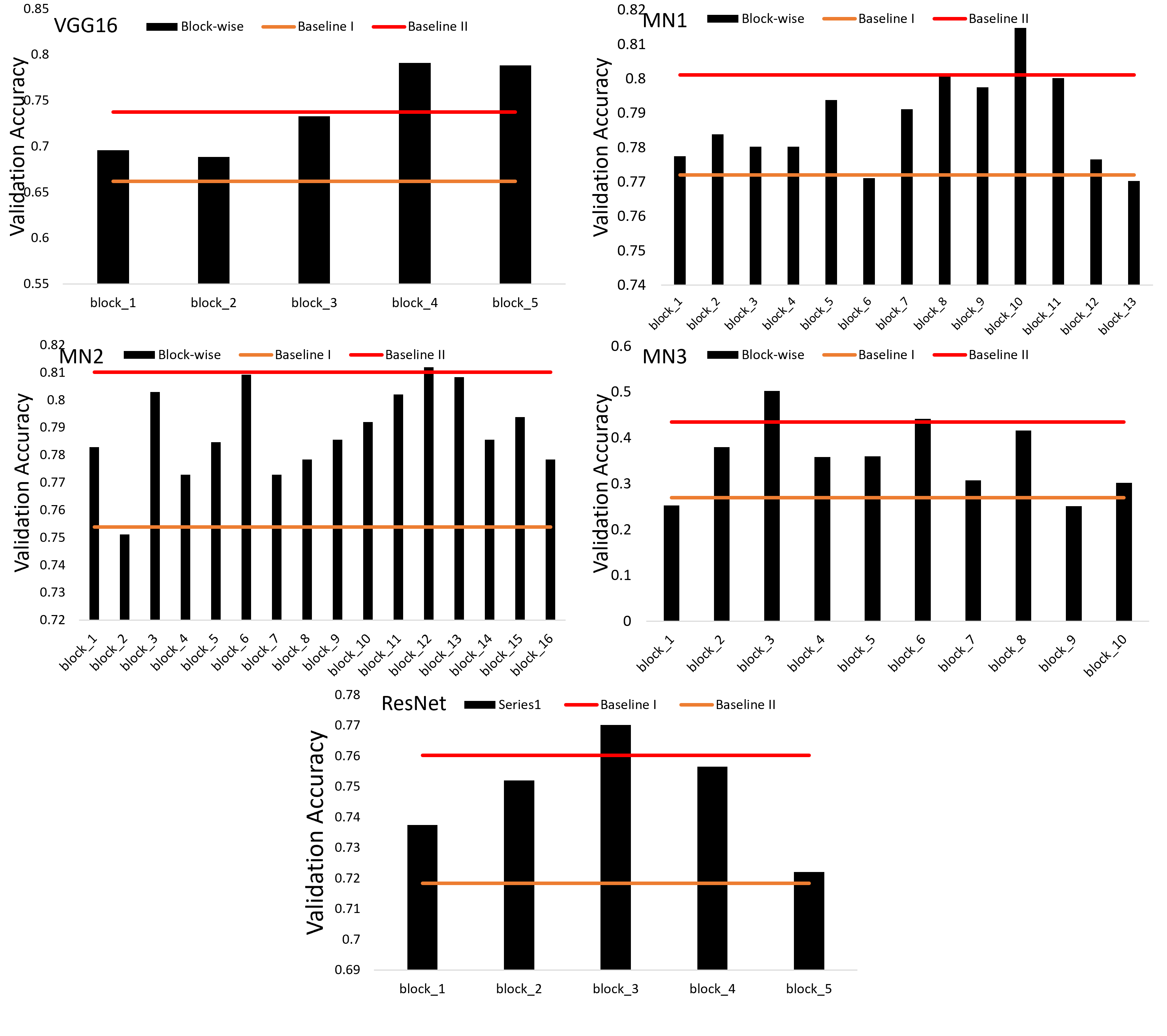
Figure 5: Block wise fine tuning accuracy using 10% of the dataset. Showing the best performing block with a white filling with vertical dash.

The next part of the investigation we evaluated the SW approach. Unlike the block-wise approach the SW approach all the blocks has a fixed number of trainable layers. Thus to asses the accuracy we had to loop through all the layers as shown in Fig. 6. Although the number of trained layers in each ‘window’ are relatively small, the achieved accuracy was comparable with the block-wise and the Baseline II approaches.

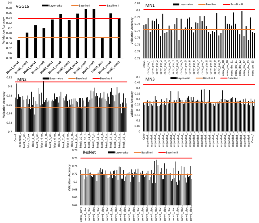
Figure 6: Sliding window fine tuning accuracy using 10% of the dataset.

To summarise we have obtained the optimal layer, block, and ‘window’ using only 10% of the data set. As shown in Fig. 7, all the tested approaches outperform Baseline I approach and few outperform Baseline II approach. Consequently we leveraged these findings to FT the models on the 70% of the dataset.

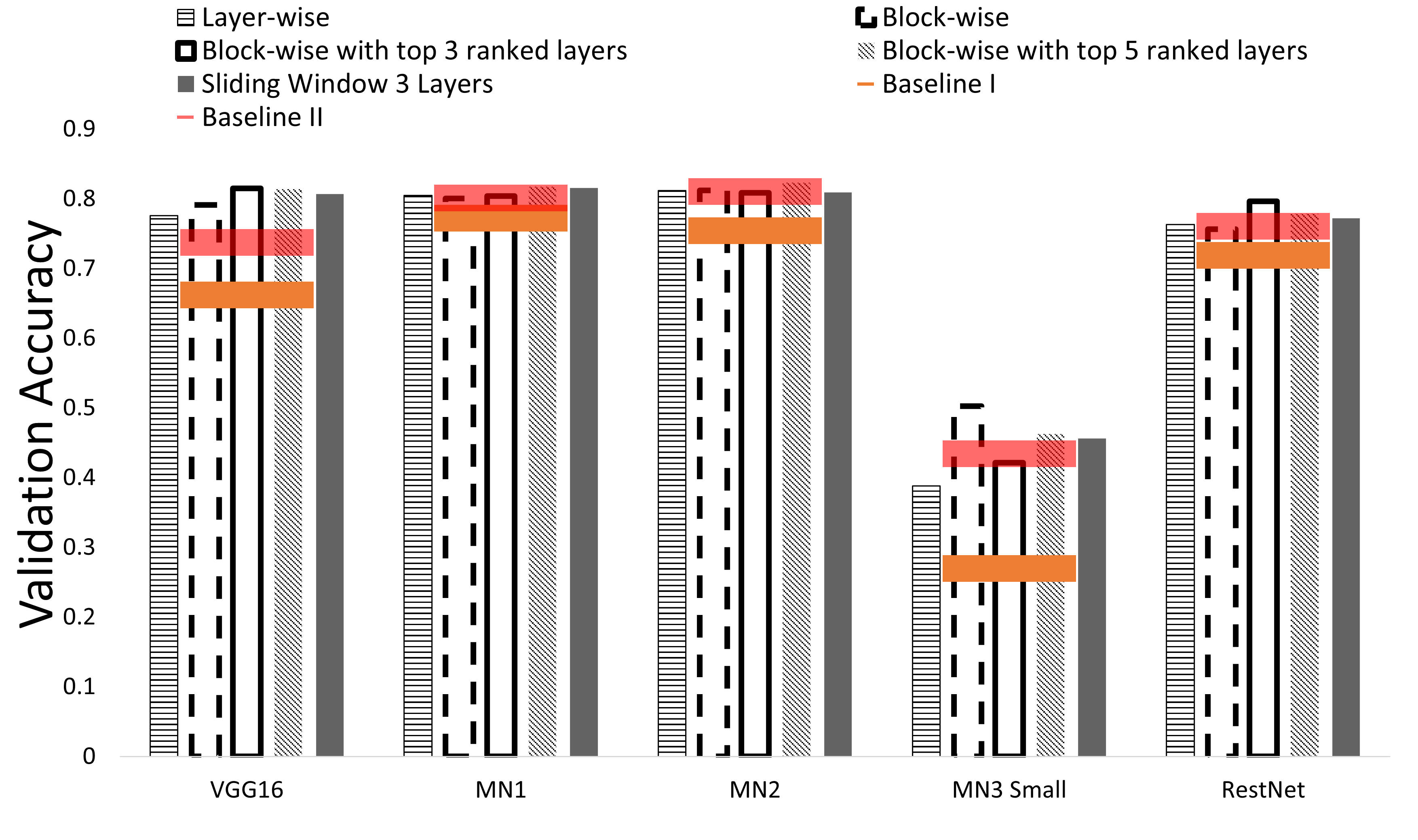
Figure 7: Fine Tuning validation accuracy using 10% of the dataset. Showing the different approaches and the baseline performance.

The fine-tinning accuracy using all the approaches using 70% of the dataset is shown in Fig. 8. We can observe that the block-wise approach had been consistent in achieving high accuracy. As it has always either score higher or equal to the Baseline II approach. To validate this findings we have repeated the experiments few time and results for the block-wise and the SW approaches are shown in AppendixVII.

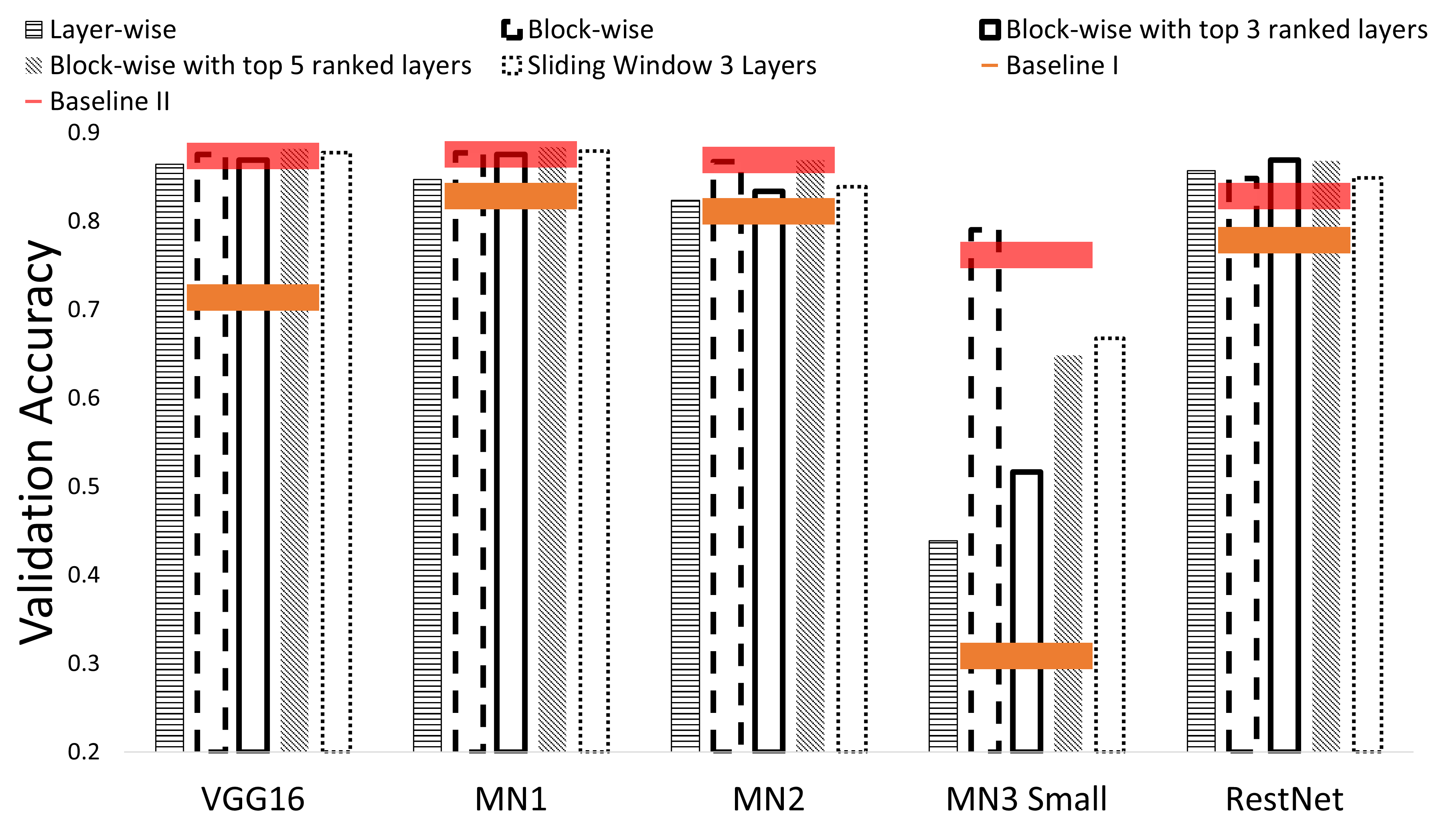
Figure 8: Block wise fine tuning accuracy using 70% of the dataset. Showing the best performing block with a white filling with vertical dash.

To evaluate the reliability and accuracy of the FT we evaluated the classification accuracy on all the models using all the baseline and proposed approaches, as show in Table I. We can observe that the Block-wise approach has the highest average validation accuracy outperforming the Baseline II approach. Moreover it has a lower accuracy variance, thus yield a consistent reliable performance.

TABLE I: Fine tuning validation accuracy showing both the mean and the variance of the tested approaches using 70% of the data. LW refers to layer-wise, BW refers to block-wise, BWT3 refers to block-wise with the 3 top ranked layers, and BWSW refers to the sliding-window approach.

	Baseline I	Baseline II	LW	BW	BWT3	BWT5	BWSW
VGG16	0.713896	0.873751	0.864668	0.875568	0.86921	0.881926	0.877384
MN1	0.828338	0.875568	0.847411	0.877389	0.875568	0.883742	0.879201
MN2	0.811081	0.86921	0.823797	0.867393	0.833787	0.86921	0.839237
MN3 Small	0.30881	0.762035	0.438692	0.790191	0.516803	0.648501	0.667575
RestNet	0.778383	0.828338	0.857402	0.848320	0.86921	0.868302	0.849228
Variance	0.046867	0.002364	0.033797	0.001318	0.024095	0.010383	0.007806
Mean	0.688102	0.84178	0.766394	0.851771	0.792916	0.830336	0.822525

VII Conclusions and future work

Our preliminary experiments suggest that randomly tuning individual layers of a pre-trained deep network can yield intriguing results, with few even outperforming traditional fine-tuning methods. We proposed a novel framework using block-wise fine-tuning to explore an efficient way to find the salient layers relevant to the features of new task data and improve fine-tuning reliability. Our proposed approach includes four different methods for determining the most salient block: layer-wise fine-tuning, layer-wise adaptation, block-wise fine-tuning, and a fixed-length sliding window. This work can be extended in several approaches such as building an automated FT approach, that can automatically identify the best performing blocks and FT them.

Appendix A Repeated experiments

To validate our findings we have repeated the experiments for the block-wise and the SW approaches. The results shown in Figs 9, and 10, shows that both approaches yield consistent performance.

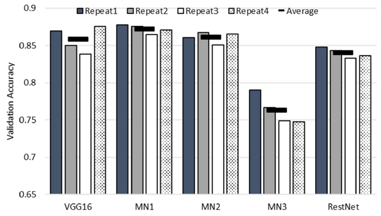
Figure 9: Block wise fine tuning accuracy using 70% of the dataset.Showing the four repeated experiment and the resulting average.

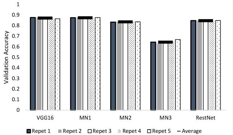
Figure 10: Sliding window fine tuning accuracy using 70% of the dataset.Showing the four repeated experiment and the resulting average.

References

- [1] Rupesh Kumar Srivastava, Klaus Greff, Jurgen Schmidhuber, “Training Very Deep Networks”, in Proceedings of the 28th International Conference on Neural Information Processing Systems, pp. 2377–2385, 2015.
- [2] Bansal, M. A., Sharma, D. R., and Kathuria, D. M. A, “Systematic review on data scarcity problem in deep learning: Solution and applications”, in ACM Computing Surveys(CSUR), 2020.
- [3] Li, H., Chaudhari, P., Yang, H., Lam, M., Ravichandran, A., Bhotika, R., and Soatto, S., “Rethinking the hyperparameters for fine-tuning”, in International Conference on Learning Representation (ICLR), 2020.
- [4] Olga Russakovsky, Jia Deng, Hao Su, Jonathan Krause, Sanjeev Satheesh, Sean Ma, Zhiheng Huang, Andrej Karpathy, Aditya Khosla, Michael Bernstein, Alexander C. Berg & Li Fei-Fei, “ImageNet Large Scale Visual Recognition Challenge”, in International Journal of Computer Vision, volume 115, pp. 211–252, 2015.
- [5] Karen Simonyan and Andrew Zisserman, “Very Deep Convolutional Networks for Large-Scale Image Recognition”, in International Conference on Learning Representations, 2015.
- [6] Christian Szegedy, Wei Liu, Yangqing Jia, Pierre Sermanet, Scott Reed, Dragomir Anguelov, Dumitru Erhan, Vincent Vanhoucke, Andrew Rabinovich, “Going deeper with convolutions”, in IEEE Conference on Computer Vision and Pattern Recognition (CVPR), pp. 1-9, 2015
- [7] Christian Szegedy, Vincent Vanhoucke, Sergey Ioffe, Jon Shlens, and Zbigniew Wojna, “Rethinking the inception architecture for computer vision”, In IEEE Conference on Computer Vision and Pattern Recognition (CVPR), pages 2818–2826, 2016.
- [8] Andrew G. Howard and Menglong Zhu and Bo Chen and Dmitry Kalenichenko and Weijun Wang and Tobias Weyand and Marco Andreetto and Hartwig Adam, “MobileNets: Efficient Convolutional Neural Networks for Mobile Vision Applications”, ArXiv, abs/1704.04861, 2017.
- [9] Kaiming He Xiangyu Zhang Shaoqing Ren Jian Sun, “Deep Residual Learning for Image Recognition”, in Computer Vision and Pattern Recognition, 2016, pp. 770–778
- [10] Yaxing Wang, Chenshen Wu, Luis Herranz, Joost van de Weijer, Abel Gonzalez-Garcia, Bogdan Raducanu, “Transferring GANs: generating images from limited data”, in European Conference on Computer Vision, pp. 220–236, 2018
- [11] Jiamei Sun, Sebastian Lapuschkin, Wojciech Samek, Alexander Binder, “Explain and Improve: LRP-Inference Fine-Tuning for Image Captioning Models”, in Information Fusion, vol.77, pp. 233–246, 2022.
- [12] Jaemin Cho, Seunghyun Yoon, Ajinkya Kale, Franck Dernoncourt, Trung Bui, Mohit Bansal, “Findings of the Association for Computational Linguistics”, in NAACL, pp. 517–527, 2022.
- [13] Zongwei Zhou, Jae Shin, Lei Zhang, Suryakanth Gurudu, Michael Gotway, and Jianming Liang, “Fine-tuning Convolutional Neural Networks for Biomedical Image Analysis: Actively and Incrementally?”, in Computer Vision and Pattern Recognition, pp. 7340–7351, 2017
- [14] Simon Kornblith, Jonathon Shlens, and Quoc V. Le., “Do better imagenet models transfer better?”, in Computer Vision and Pattern Recognition (CVPR), pp. 2661–2671, 2019.
- [15] M. Tanveer, M. Karim Khan and C. Kyung, “Fine-Tuning DARTS for Image Classification”, in International Conference on Pattern Recognition (ICPR), pp. 4789–4796, Milan, Italy, 2021.
- [16] Heechul Jung Sihaeng Lee Junho Yim Sunjeong Park Junmo Kim, “Joint Fine-Tuning in Deep Neural Networks for Facial Expression Recognition”, in International Conference on Computer Vision, pp. 2983-2991, 2015.
- [17] Younmgin Ro1, Jin Young Choi, “AutoLR: Layer-wise Pruning and Auto-tuning of Learning Rates in Fine-tuning of Deep Networks”, in AAAI Conference on Artificial Intelligence, pp. 2486–2494, 2021
- [18] Hamdi, S., Snoussi, H., Abid, M., “Fine-Tuning a Pre-trained CAE for Deep One Class Anomaly Detection in Video Footage”, in Pattern Recognition and Artificial Intelligence, Communications in Computer and Information Science, vol 1322. Springer, 2020.
- [19] Rippel, O., Chavan, A., Lei, C., and Merhof, D., “Transfer Learning Gaussian Anomaly Detection by Fine-Tuning Representations”, in ArXiv, abs/2108.04116., 2021.
- [20] Jhih-Ciang Wu, Ding-Jie Chen, Chiou-Shann Fuh, and Tyng-Luh Liu, “Learning Unsupervised Metaformer for Anomaly Detection”, in International Conference on Computer Vision, pp. 4369–4378, 2021.
- [21] Jian Xu, Cunzhao Shi, Chengzuo Qi, Chunheng Wang, Baihua Xiao, “Unsupervised Part-Based Weighting Aggregation of Deep Convolutional Features for Image Retrieval”, in Proceedings of the AAAI Conference on Artificial Intelligence, pp. 7436–7443, vol.32, no.1, 2018.
- [22] F. Radenović, G. Tolias and O. Chum, “Fine-Tuning CNN Image Retrieval with No Human Annotation”, in IEEE Transactions on Pattern Analysis and Machine Intelligence, vol. 41, no. 7, pp. 1655–1668, 2019.
- [23] C. Liu, B. Zoph, M. Neumann, J. Shlens, W. Hua, L.-J. Li, L. Fei-Fei, A. Yuille, J. Huang, and K. Murphy, “Progressive neural architecture search”, in Lecture Notes in Computer Science, pp. 1–16, 2018.
- [24] H. Pham, M. Y. Guan, B. Zoph, Q. V. Le, J. Dean, “Efficient neural architecture search via parameter sharing”, in Proc. of the International Conference on Machine Learning, pp. 4092–4101, 2018
- [25] Z. Lu, G. Sreekumar, E. D. Goodman, W. Banzhaf, K. Deb, V. N. Boddeti, “Neural architecture transfer”, in IEEE transactions on pattern analysis and machine intelligence, vol.43, no.9, pp. 2971–2989, 2021.
- [26] Youngkee Kim, Won Joon Yun, Youn Kyu Lee, Soyi Jung, Joongheon Kim, “Two-stage architectural fine-tuning with neural architecture search using early-stopping in image classification”, in https://doi.org/10.48550/arXiv.2202.08604, 2022.
- [27] Yosinski, J., Clune, J., Bengio, Y., and Lipson, H., “How transferable are features in deep neural networks?”, in Advances in neural information processing systems, pp. 3320–3328, 2014.
- [28] Zeiler, M. D., Fergus, R., “Visualizing and understanding convolutional networks”, in The European Conference on Computer Vision (ECCV), pp. 818–833, 2014.
- [29] Tajbakhsh, N., Shin, J. Y., Gurudu, S. R., Hurst, R. T., Kendall, C. B., Gotway, M. B., and Liang, J., “Convolutional neural networks for medical image analysis: Full training or fine tuning?”, in IEEE transactions on medical imaging vol.35(5), pp. 1299–1312, 2016.
- [30] Guo, Y., Shi, H., Kumar, A., Grauman, K., Rosing, T., and Feris, R., “SpotTune: transfer learning through adaptive fine-tuning”, in Proceedings of the IEEE conference on computer vision and pattern recognition (CVPR), pp. 4805–4814, 2019.
- [31] Tanvir Mahmud and Natalia Frumkin and Diana Marculescu, “RL-Tune: A Deep Reinforcement Learning Assisted Layer-wise Fine-Tuning Approach for Transfer Learning”, in First Workshop on Pre-training: Perspectives, Pitfalls, and Paths Forward at ICML, 2022.
- [32] Bharat Singh and Soham De and Yangmuzi Zhang and Thomas A. Goldstein and Gavin Taylor, “Layer-Specific Adaptive Learning Rates for Deep Networks”, in IEEE 14th International Conference on Machine Learning and Applications (ICMLA), pp. 364–368, 2015
- [33] Kornblith, S., Shlens, J., and Le, Q. V., “Do better imagenet models transfer better?”, in Proceedings of the IEEE/CVF conference on computer vision and pattern recognition, pp. 2661–2671, 2019.
- [34] Parker-Holder, J., Nguyen, V., and Roberts, S. J., “Provably efficient online hyperparameter optimization with population-based bandits”, in Advances in Neural Information Processing Systems, vol.33, pp. 17200–17211, 2020.
- [35] Bottou, Léon, Bousquet, Olivier, “The Tradeoffs of Large Scale Learning”, In Optimization for Machine Learning, Cambridge, MIT Press. pp. 351–368, 2012.
- [36] Kingma, D. P., Ba, L. J., “Adam: A method for Stochastic Optimization”, in International Conference on Learning Representations (ICLR), 2015.
- [37] Alexey Dosovitskiy, Lucas Beyer, Alexander Kolesnikov, Dirk Weissenborn, Xiaohua Zhai, Thomas Unterthiner, Mostafa Dehghani, Matthias Minderer, Georg Heigold, Sylvain Gelly, Jakob Uszko- reit, and Neil Houlsby, “An image is worth 16x16 words: Transformers for image recognition at scale”, in International Conference on Learning Representations (ICLR), 2021.
- [38] Ananya Kumar, Aditi Raghunathan, Robbie Jones, Tengyu Ma, and Percy Liang, “Fine-tuning can distort pretrained features and underperform out-of-distribution”, in International Conference on Learning Representations (ICLR), 2022
- [39] Ilya Loshchilov and Frank Hutter, “Decoupled weight decay regularization”, in International Conference on Learning Representations, 2019.
- [40] Kumar, Ananya and Shen, Ruoqi and Bubeck, Sébastien and Gunasekar, Suriya, “How to Fine-Tune Vision Models with SGD”, in https://arxiv.org/abs/2211.09359, 2022
- [41] Jeremy Howard and Sebastian Ruder, “Universal Language Model Fine-tuning for Text Classifier”, in Proceedings of the 56th Annual Meeting of the Association for Computational Linguistics, pp. 328–339, 2018.
- [42] Tomas Mikolov, Kai Chen, Greg Corrado, and Jeffrey Dean, “Distributed Representations of Words and Phrases and their Compositionality”, in Advances in Neural Information Processing Systems, pp. 3111–3119, 2013.
- [43] Brown, T., Mann, B., Ryder, N., Subbiah, M., Kaplan, J. D., Dhariwal, P., Neelakantan, A., Shyam, P., Sastry, G., Askell, A., et al., “Language models are few-shot learners”, in Advances in Neural Information Processing Systems, 2020.
- [44] Teven Le Scao, Angela Fan, Christopher Akiki, Ellie Pavlick, Suzana Ilic et al., “BLOOM: A 176B-Parameter Open-Access Multilingual Language Model”, in https://doi.org/10.48550/arXiv.2211.05100, 2022.
- [45] Fedus, W., Zoph, B., and Shazeer, N., “Switch transformers: Scaling to trillion parameter models with simple and efficient sparsity”, in Journal of Machine Learning Research, vol.23, pp. 1–39, 2022.
- [46] Li, X. L. and Liang, P., “ Prefix-tuning: Optimizing continuous prompts for generation”, in 59th Annual Meeting of the Association for Computational Linguistics and the 11th International Joint Conference on Natural Language Processing, pp. 4582–4597, 2021.
- [47] He, J., Zhou, C., Ma, X., Berg-Kirkpatrick, T., and Neubig, G., “Towards a unified view of parameter-efficient transfer learning”, in International Conference on Learning Representations (ICLR), 2022.
- [48] Xinhsuai Dong, Luu Anh Tuan, Min Lin, Shuicheng Yan, Hanwang Zhang, “How Should Pre-Trained Language Models Be Fine-Tuned Towards Adversarial Robustness?”, in 35th Conference on Neural Information Processing System, 2021.
- [49] Fatemehsadat Mireshghallah, Archit Uniyal, Tianhao Wang, David Evans, Taylor Berg-Kirkpatrick, “Memorization in NLP Fine-tuning Methods”, in https://doi.org/10.48550/arXiv.2205.12506, 2022.
- [50] Wen-Chin Huang and Chia-Hua Wu and Shang-Bao Luo and Kuan-Yu Chen and Hsin-Min Wang and Tomoki Toda, “Speech Recognition by Simply Fine-Tuning Bert”, in ICASSP 2021 - 2021 IEEE International Conference on Acoustics, Speech and Signal Processing (ICASSP), pp. 7343–7347, 2021.
- [51] Violeta, L., Ma, D., Huang, Wen-Chin and Toda, T., “Intermediate Fine-Tuning Using Imperfect Synthetic Speech for Improving Electrolaryngeal Speech Recognition”, in 10.48550/arXiv.2211.01079, 2022
- [52] Ioannis Tsiamas, Gerard I. Gállego, Carlos Escolano, José A. R. Fonollosa, Marta R. Costa-jussà, “Pretrained Speech Encoders and Efficient Fine-tuning Methods for Speech Translation: UPC at IWSLT 2022”, in Proceedings of the 19th International Conference on Spoken Language Translation (IWSLT 2022), pp. 265–276, 2022.
- [53] Séverine Guillaume, Guillaume Wisniewski, Cécile Macaire, “Fine-tuning pre-trained models for Automatic Speech Recognition: experiments on a fieldwork corpus of Japhug”, in Proceedings of the Fifth Workshop on the Use of Computational Methods in the Study of Endangered Languages, pp. 170–178, 2022.
- [54] Jan Vanek, Josef Michálek and Josef Psutka, “Tuning of Acoustic Modeling and Adaptation Technique for a Real Speech Recognition Task”, in International Conference on Statistical Language and Speech Processing, pp. 235–245, 2019.
- [55] Linkai Peng, Kaiqi Fu, Binghuai Lin, Dengfeng Ke, Jinsong Zhang, “A study on fine-tuning wav2vec2.0 Model for the task of Mispronunciation Detection and Diagnosis”, in InterSpeech, pp. 4448–4451, 2021.
- [56] Haidar, M. A. and Rezagholizadeh, M., “Fine-Tuning of Pre-Trained End-to-End Speech Recognition with Generative Adversarial Networks”, in IEEE International Conference on Acoustics, Speech and Signal Processing (ICASSP), pp. 6204–6208, 2021.
- [57] Goodfellow, Ian etc., “Generative Adversarial Nets”, in Proceedings of the International Conference on Neural Information Processing Systems, pp. 2672–2680, 2014.
- [58] The TensorFlow Team, tfflowers, ‘http://download.tensorflow.org/example_images/flower_photos.tgz’, Jan., 2019
- [59] Saini, M., Susan, S. Bag-of-Visual-Words codebook generation using deep features for effective classification of imbalanced multi-class image datasets. Multimed Tools Appl 80, 20821–20847 (2021). https://doi.org/10.1007/s11042-021-10612-w
- [60] Howard, A. G., Zhu, M., Chen, B., Kalenichenko, D., Wang, W., Weyand, T., Andreetto, M., ; Adam, H. (2017). MobileNets: Efficient Convolutional Neural Networks for Mobile Vision Applications. https://doi.org/10.48550/arxiv.1704.04861
- [61] A. Howard et al., ”Searching for MobileNetV3,” 2019 IEEE/CVF International Conference on Computer Vision (ICCV), Seoul, Korea (South), 2019, pp. 1314-1324, doi: 10.1109/ICCV.2019.00140.
- [62] Keras, ‘Dropout layer’. Retrieved January 13, 2023, from https://keras.io/api/layers/regularization_layers/dropout/
- [63] Keras, ‘Flatten layer’. Retrieved January 13, 2023, from https://keras.io/api/layers/reshaping_layers/flatten/
- [64] Keras, ‘Dense layer’. Retrieved January 13, 2023, from https://keras.io/api/layers/core_layers/dense/
- [65] Chollet, F., 2021. Deep learning with Python. Simon and Schuster.
- [66] Goodfellow, I., Bengio, Y. and Courville, A., 2016. ‘Deep learning’. MIT press.
- [67] Srivastava, N., Hinton, G., Krizhevsky, A., Sutskever, I. and Salakhutdinov, R., 2014. Dropout: a simple way to prevent neural networks from overfitting. The journal of machine learning research, 15(1), pp.1929-1958.