Optical characterization and Radial velocity monitoring with Belgian and Indian Telescopes (ORBIT): the eclipsing binaries EPIC 211982753 and EPIC 211915147

Abstract

The K2 eclipsing binary candidates EPIC 211982753 (hereinafter called EPIC2753) and EPIC 211915147 (hereinafter called EPIC5147) are characterized with the help of photometric and high-resolution spectroscopic data. The light curve analysis uses the $R_{c}$-band photometric data from the 1.3-m Devasthal Fast Optical Telescope (DFOT, India), ASAS-3 and K2 observations. High-resolution échelle spectra are collected using the HERMES spectrograph at the 1.2-m MERCATOR telescope (La Palma, Spain). The synthetic light and radial velocity curves are generated with the help of the modeling package PHOEBE 1.0. The orbital period analysis based on the $\sim$3.2 years of K2 observations does not show any change in the orbital period of both targets. The component masses $M_{1,2}$ are estimated as 1.69(0.02) and 1.59(0.02) $M_{\odot}$ for EPIC2753, and 1.48(0.01) and 1.27(0.01) $M_{\odot}$ for EPIC5147. Both systems are high mass-ratio eclipsing binaries with q>0.85. The component radii $R_{1,2}$ are found to be 1.66(0.02) and 1.53(0.02) $R_{\odot}$ for EPIC2753, and 1.80(0.05) and 1.42(0.05) $R_{\odot}$ for EPIC5147. The distances of EPIC2753 and EPIC5147 are determined as 238(4) and 199(5) pc, respectively. MESA Isochrones and Stellar Tracks are used to understand the evolutionary status of both systems.

1 Introduction

The stellar parameter determination is more precise and easier in the case of eclipsing binaries (EBs) as compared to single stars. Both photometric and spectroscopic observations are required for a complete orbital solution and direct parameter determination of EBs. In addition to the accurate fundamental parameters, EBs offer a way to explore the interaction between the components, evolution and formation of multiple systems, distance measurements, etc. Masses and radii determined using double-lined eclipsing binaries can be accurate up to 3$\%$ depending on the quality of photometric and spectroscopic data (Torres et al., 2010). The information about luminosity ratio, radius ratio, inclination, orbital period ($P_{\rm orb}$) and eccentricity is derived from photometric time series. The multi-epoch radial velocity (RV) data give information about the mass ratio (q=$m_{2}/m_{1}$) of the system. The use of long-term photometric observations is required to detect any $P_{\rm orb}$ variation signatures which can be used further to reveal underlying mechanisms for the observed $P_{\rm orb}$ change. The $P_{\rm orb}$ analysis is used to understand the processes of mass transfer, magnetic cycles as well as to infer the presence of any additional component in the system. There are thousands of EBs discovered by different ground- and space-based surveys during the last two decades (Street et al., 2003; Borucki et al., 2010; Ricker et al., 2015). The high-precision and long-term continuous photometric observations by the space missions Kepler/K2 (Borucki et al., 2010) and TESS (Ricker et al., 2015) offer additional opportunities to study stellar activity, pulsation and $P_{\rm orb}$ evolution of EB components. However RV data are unavailable for most of these systems.

On the basis of Roche lobe geometry, the EBs are divided into detached, semi-detached and contact systems. In detached binaries, radius of each component is smaller than Roche surface. In case of semi-detached systems, one of the components fills its Roche lobe whereas both components are found to fill or over-fill their Roche lobes in contact binaries. Due to the the large distance between the components of widely detached binaries, the components do not interact with each other during their evolution. The binary components in such systems evolve independently of each other like an isolated star (Hurley et al., 2002) and follow standard models of stellar evolution. Binaries are believed to be formed by fragmentation or from third-body capture (Fabian et al., 1975; Goodwin et al., 2004; Bodenheimer, 2011; Moe & Di Stefano, 2017). Contact binary systems are formed from short-period detached or semi-detached systems via angular momentum loss (Okamoto & Sato, 1970; Bate et al., 2002; Tokovinin & Moe, 2020). The precise parameters of the components of EB systems can be used for testing stellar evolution models as well as to study multiple system evolution (Higl & Weiss, 2017).

The systems EPIC2753 (= HD 69735) and EPIC5147 (= HD 73470) were both detected thanks to the STEREO mission of NASA. Wraight et al. (2011) reported 163 EBs with brightness less than 10.5 mag. Out of these 163 EBs, 122 systems (including EPIC2753) were newly reported. Wraight et al. (2012) analyzed the STEREO spacecraft data with a matched filter algorithm to detect low-amplitude signals. A total of nine low-mass EBs were detected while some other systems (including EPIC5147) were reported as potential follow-up sources due to their grazing eclipse features. Both systems are mentioned as EB candidates in Barros et al. (2016), who searched the K2 data (C1 to C6) for transit signals using a modified version of the CoRoT alarm pipeline. Barros et al. (2016) reported 172 planetary and 327 EB candidates from K2 data for follow-up observations.

In the framework of the Belgo-Indian Network for Astronomy & Astrophysics (BINA) project, we have initiated a long-term programme called "Optical characterization and Radial velocity monitoring with Belgian and Indian Telescopes (ORBIT)" which aims at collecting ground-based photometric and high-resolution spectroscopic observations of few selected low-mass eclipsing binary and exoplanet candidates to perform an in-depth characterization of their physical nature (Joshi et al., 2019).

In this paper, the fundamental stellar parameters of the two systems are derived using light curves (LCs) and RV curves fitting. The systems have not been investigated in any previous studies. The basic information about the targets collected in different surveys is given in Table 1. The outline of the paper is as follows. The detailed observations concerning the targets are given in § 2. In § 3, we update the ephemeris of both systems. The radial velocities are derived in § 4. The modeling work has been carried out in § 5. Finally, we discuss the results in § 6.

Table 1: Basic information about EPIC2753 and EPIC5147 taken from different surveys.

Parameter	EPIC2753	EPIC5147	Reference
RA (∘)	124.7503	129.7887	Barros et al. (2016)
DEC (∘)	+19.9760	+18.9519	Barros et al. (2016)
Period (days)	5.389631	1.811266	Barros et al. (2016)
B (mag)	9.067 $\pm$ 0.014	9.255 $\pm$ 0.021	Høg et al. (2000)
V (mag)	8.769 $\pm$ 0.014	8.815 $\pm$ 0.021	Høg et al. (2000)
R (mag)	8.541	8.500	Bourges et al. (2017)
I (mag)	8.428	8.327	Bourges et al. (2017)
J (mag)	8.236 $\pm$ 0.027	8.082 $\pm$ 0.018	Cutri et al. (2003)
H (mag)	8.180 $\pm$ 0.017	7.923 $\pm$ 0.029	Cutri et al. (2003)
K (mag)	8.154 $\pm$ 0.018	7.893 $\pm$ 0.029	Cutri et al. (2003)
L (mag)	8.135 $\pm$ 0.022	7.814 $\pm$ 0.027	Cutri et al. (2012)
M (mag)	8.147 $\pm$ 0.019	7.851 $\pm$ 0.021	Cutri et al. (2012)
N (mag)	8.167 $\pm$ 0.021	7.855 $\pm$ 0.025	Cutri et al. (2012)
$A_{V}$ (mag)	0.116 $\pm$ 0.006	0.063 $\pm$ 0.003	Schlafly & Finkbeiner (2011)
$\pi$ (mas)	4.033 $\pm$ 0.021	4.851 $\pm$ 0.020	Gaia Collab. (2021)

2 Observations

2.1 Photometry

The 1.3-m Devasthal Fast Optical Telescope (DFOT) was used for photometric follow-up observations. The $2k\times 2k$ conventional back-illuminated CCD camera with a gain of $2e^{-}ADU^{-1}$ and a read-out noise of $7.5e^{-}$ was used during the observations. The field of view (FoV) of $\sim 18^{\arcmin}\times 18^{\arcmin}$ provides multiple comparison stars in the vicinity of target stars. EPIC2753 was observed in the $R_{c}$ band during primary eclipse on three different nights. The system EPIC5147 was observed for $\sim$45 hours on different nights in the $R_{c}$ band covering both primary and secondary eclipse. The observation log for the targets using the 1.3-m DFOT is given in Table 2. The raw telescope images were cleaned with the help of standard IRAF routines. The AstroImageJ (AIJ) software package (Collins et al., 2017) was used to extract the target and comparison star fluxes from the science images using the technique of aperture photometry. For EPIC2753, TIC 14435258 and TIC 14433509 were used as comparison and check star, respectively. The field stars TIC 175233354 and TIC 175233313 were used as comparison and check star, respectively, for EPIC5147.

Table 2: The 1.3  m $R_{c}$-band observation log for EPIC2753 (upper block) and EPIC5147 (lower block).

Date of	Start BJD	End BJD	Total	Exposure	Obs.
obs.			frames		time
	(2450000+)	(2450000+)		(sec)	(hrs)
20190110	8494.4059	8494.4970	239	20	2.19
20190428	8602.1411	8602.1744	198	05	0.80
20200319	8928.1715	8928.2522	499	05	1.94
20201230	9214.2692	9214.4177	1235	05	3.56
20210217	9263.0746	9263.1215	449	02	1.13
20210217	9263.2215	9263.2583	399	02	0.88
20220130	9610.1959	9610.4427	2759	02	5.92
20220201	9612.1165	9612.2528	1499	02	3.27
20220219	9630.0895	9630.3289	2639	02	5.75
20220301	9640.1629	9640.3570	505	02	4.66
20220307	9646.3134	9646.3616	470	02	1.16
20220310	9649.1266	9649.1467	209	02	0.48
20220318	9657.0656	9657.2849	2066	02	5.26
20220319	9658.2724	9658.2803	90	02	0.19
20220320	9659.0596	9659.3042	2729	02	5.87
20220414	9684.1458	9684.1658	175	02	0.48
20220415	9685.0783	9685.0987	175	02	0.49
20220416	9686.0855	9686.1109	280	02	0.61
20220417	9687.0903	9687.1027	140	02	0.30
20200213	8893.2185	8893.3898	1015	03	4.11
20200224	8904.2490	8904.3287	500	05	1.91
20211207	9556.2522	9556.5157	2100	03	6.32

The Kepler mission was launched by NASA in 2009 to detect exoplanets in the Cygnus-Lyra region of the Milky Way (Borucki et al., 2010). The mission observed $\sim$150,000 stars with a 30 and 1 minute cadence during the prime mission period up to November 2012. The Kepler spacecraft lost two reaction wheels by May 2013 which affected its pointing accuracy. After a redefinition of the goals, the second phase of mission, referred to as K2 , started in May 2014 and lasted for another four years. The K2 mission observed in total 21 campaign fields close to the ecliptic equator (C00, C01, C02,…, C19). All of them, except C00, were observed for approximately 80 days. Both the Kepler and K2 observations were done through a spectral bandpass from 400 to 850 nm. The data of the observed targets are available at the Barbara A. Mikulski Archive for Space Telescopes (MAST) and the NASA Exoplanet Archive. EPIC2753 was observed by K2 for 74 and 49 days during C05 and C18, respectively. The system EPIC7147 was observed by K2 during the campaigns C05, C16 and C18 for almost 75, 80 and 51 days, respectively. The available photometric time series were corrected for the spacecraft’s pointing errors with the EPIC Variability Extraction and Removal for Exoplanet Science Targets (EVEREST) pipeline (Luger et al., 2016). The K2 observation log is given in Table 3.

Both the systems were observed by the All Sky Automated Survey (ASAS-3) from December 2002 to December 2009. The ASAS-3 is installed in Las Campanas Observatory and operated by Carnegie Institution of Washington (Pojmański, 2001). Most of the observations were done in V band. For EPIC2753, $\sim$ 475 data points were available and $\sim$ 400 data points had good quality according to given flags. Similarly, for EPIC5147, $\sim$ 450 data points were given good quality flag out of total 565 data points. The data points with large uncertainty and poor photometric quality were excluded during analysis.

Table 3: The K2 observation log for EPIC2753 and EPIC5147.

K2	BJDstart	BJDend	Data	Exposure	Reduction
Campaign	(2450000+)	(2450000+)	points	(seconds)	Pipeline
EPIC2753
C05	7140.5502	7214.4109	3402	1800	EVEREST
C18	8253.2213	8302.3801	2265	1800	EVEREST
EPIC5147
C05	7139.6107	7214.4318	3663	1800	EVEREST
C16	8095.4678	8175.0229	3894	1800	EVEREST
C18	8251.5462	8302.4010	2490	1800	EVEREST

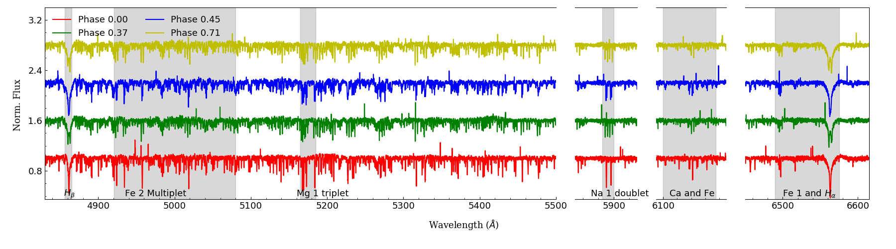
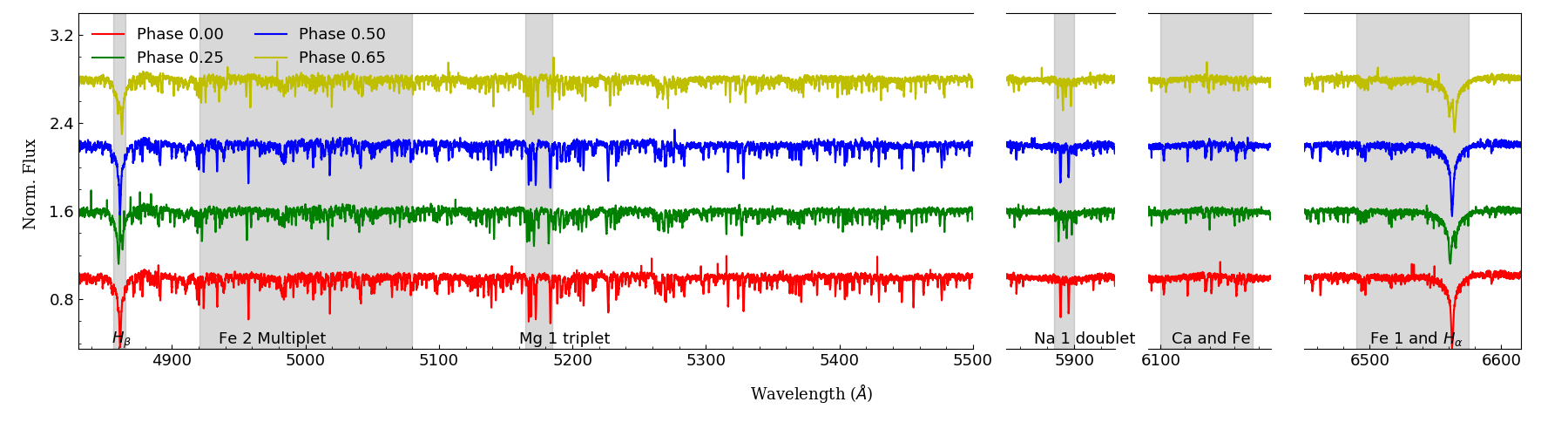
Figure 1: Sample spectra for EPIC2753 (upper) and EPIC5147 (lower) at different phases as observed using the HERMES spectrograph. Some spectral line groups are shown by shaded regions. The normalized spectra are vertically shifted for more clarity and the phases are given in upper left corner of each plot.

2.2 High Resolution Spectroscopy

The systems EPIC2753 and EPIC5147 were observed using the High-Efficiency and high-Resolution Mercator Echelle Spectrograph (HERMES) mounted at the 1.2-m Mercator Telescope at the Roque de los Muchachos observatory on the Canary island La Palma in Spain (Raskin et al., 2011). This high-resolution fibre-fed spectrograph provides a spectral coverage of 380-900 nm and a spectral resolution of $\sim$85 000 in the high-resolution mode. A standard-silicon, thinned, back-illuminated 2048 $\times$ 4608 pixels CCD is used for recording the spectra. Both sources were observed in the simultaneous wavelength reference mode (HRF-WRF). Ten spectra were collected for EPIC2753 between 4 January to 7 February in 2019. For EPIC5147, 18 spectra were collected from 4 January to 26 February in 2019. The HERMES data reduction pipeline (DRS) V 5.0 was used for the reduction of the data. The normalisation was done with spline interpolation from the Python library SciPy. The overlapping region from adjacent orders was removed before combining all the orders in single spectra. Fig. 1 shows a selection of representative wavelength regions of the resulting normalised HERMES spectra of EPIC2753 and EPIC5147 at four different orbital phases.

3 Updating Ephemeris

The K2 time series is used to obtain initial estimates of the $P_{\rm orb}$ of each source. The photometric precision of the K2 data is better than that of the DFOT and ASAS-3 ground-based observations. Furthermore, continuous observations of the targets are available for many days (50-70 days) in the K2 survey. All the available data sets from different K2 campaigns are combined to determine the $P_{\rm orb}$. The $P_{\rm orb}$ of each system is determined using the Period04 program. This program uses the discrete Fourier transform algorithm for the analysis of large time series with gaps (Lenz & Breger, 2005). The $P_{\rm orb}$ determination and its evolution in time are discussed in the following sections.

3.1 EPIC2753

The $P_{\rm orb}$ of the system is determined as 5.390094 $\pm$ 0.000241 days using Period04. This value is in agreement with the 5.389631 days period reported by Barros et al. (2016). During the O-C analysis, we used HJD 2457141.732244 as the time of minimum brightness (TOM) at epoch 0. The orbital cycle numbers are calculated using the 5.390094 days period. The stability of $P_{\rm orb}$ can be studied through an $(O-C)$-diagram. For this purpose, we calculated the TOMs from the K2 data using a quadratic (parabola) fitting in the minima regions of the light curve (LC).

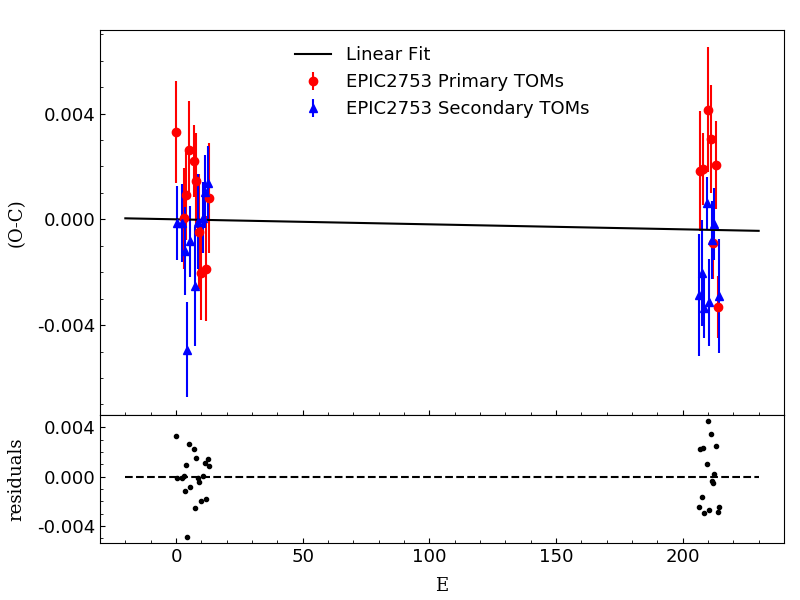
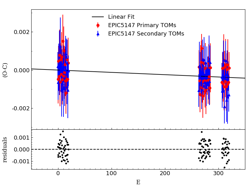
Figure 2: O-C diagram for EPIC2753 (upper) and EPIC5147 (lower) with linear fit.

We thus determined 35 TOMs (17 primary TOMs + 18 secondary TOMs) for EPIC2753 from the K2 data. The updated linear ephemeris of the system can be described by the following equation:

$$HJD_{o}(E)= 2457141.7289(\pm 0.0005)$$ (1)

$$+5.389918(\pm 0.000004)\times E$$

where, HJD_o(E) represents Heliocentric Julian date at the primary minimum of the orbital cycle number E. The upper panel of Fig. 2 shows the best fit to E versus the O-C data with the residuals. The red and blue markers represent the primary and secondary minima, respectively. The O-C diagram does not show any variation and can be represented by the linear equation:

$$(O-C)= -0.237836(\pm 508.62)\times 10^{-6}$$ (2)

$$-1.89206(\pm 3.68891)\times 10^{-6}\times E$$

Here, O-C is the difference between the observed and calculated $E^{th}$ TOM for the system in days. This fit is statistically equivalent with (O-C)=0 (as the errors on both variables are much larger than the values themselves), leading to the conclusion that the $P_{\rm orb}$ is constant. The time basis available to us is only 200 cycles or  3.2 yrs which is insufficient to reveal any period change caused by long term effects such as magnetic activity cycles or extra components. The information concerning TOMs, errors, orbital cycles, minima, O-C and their residuals is given in Table 4.

Table 4: Eclipse minima timings for EPIC2753 derived using Kepler/K2  data from campaign 05 and 18 observation.

HJD∘	Error	Cycle	Min	O-C	residuals
(2450000+)				(days)	(days)
7141.732244	0.001928	000.0	p	0.003308	0.0033082
7144.423768	0.001394	000.5	s	-0.000128	-0.0001268
7155.203596	0.001485	002.5	s	-0.000140	-0.0001350
7157.898731	0.001898	003.0	p	0.000035	0.0000409
7160.592458	0.001668	003.5	s	-0.001198	-0.0011911
7163.289521	0.001684	004.0	p	0.000905	0.0009128
7165.978647	0.001798	004.5	s	-0.004929	-0.0049202
7168.681164	0.001862	005.0	p	0.002628	0.0026377
7171.372661	0.001336	005.5	s	-0.000835	-0.0008243
7179.460596	0.001361	007.0	p	0.002220	0.0022335
7182.150805	0.002250	007.5	s	-0.002531	-0.0025166
7184.849762	0.001789	008.0	p	0.001466	0.0014814
7187.543161	0.001797	008.5	s	-0.000095	-0.0000787
7190.237754	0.002160	009.0	p	-0.000462	-0.0004447
7195.626125	0.001812	010.0	p	-0.002011	-0.0019918
7198.323152	0.001343	010.5	s	0.000056	0.0000761
7203.714058	0.001381	011.5	s	0.001042	0.0010640
7206.406114	0.001982	012.0	p	-0.001862	-0.0018391
7209.104306	0.001406	012.5	s	0.001370	0.0013939
7211.798695	0.002085	013.0	p	0.000799	0.0008238
8254.744561	0.002299	206.5	s	-0.002855	-0.0024640
8257.444191	0.002275	207.0	p	0.001815	0.0022069
8260.135310	0.002012	207.5	s	-0.002026	-0.0016332
8262.834198	0.001370	208.0	p	0.001902	0.0022958
8265.523910	0.001143	208.5	s	-0.003346	-0.0029513
8270.917781	0.000999	209.5	s	0.000605	0.0010016
8273.616284	0.002348	210.0	p	0.004148	0.0045456
8276.303955	0.001642	210.5	s	-0.003141	-0.0027425
8279.005077	0.002043	211.0	p	0.003021	0.0034205
8281.696244	0.001474	211.5	s	-0.000772	-0.0003716
8284.391084	0.001375	212.0	p	-0.000892	-0.0004906
8287.086759	0.001343	212.5	s	-0.000177	0.0002253
8289.783954	0.001663	213.0	p	0.002058	0.0024613
8295.168500	0.001172	214.0	p	-0.003316	-0.0029109
8297.863873	0.002144	214.5	s	-0.002903	-0.0024969

3.2 EPIC5147

The $P_{\rm orb}$ for the system is calculated as 3.62149 $\pm$ 0.00007 days using Period04, which is almost twice the $P_{\rm orb}$ reported by Barros et al. (2016). The latter was derived using C05 data only as the other data sets (C16 and C18) were not available at that time. The orbital cycle numbers for the O-C analysis are calculated using the 3.62149 days period. We used HJD 2457142.197474 as the time of minimum brightness (TOM) at epoch 0.

Using the K2 data, we determined 111 TOMs (54 primary TOMs + 57 secondary TOMs) for the system. The updated linear ephemeris of the system can be described by the following straight line equation:

$$HJD_{o}(E)= 2457142.1975(\pm 0.0001)$$ (3)

$$+3.6215398(\pm 0.0000004)\times E$$

where, HJD_o is Heliocentric Julian date at the primary minimum of the orbital cycle number E. The lower panel of Fig. 2 shows the E versus O-C data for EPIC5147 with the best-fit line and the residuals. The red and blue markers represent the primary and secondary minima, respectively. The O-C diagram does not show any variation and can be represented by the linear equation:

$$(O-C) =4.777081(\pm 1018.9)\times 10^{-7}$$ (4)

$$-1.21(\pm 0.44)\times 10^{-7}\times E$$

The analysis shows the stable nature of $P_{\rm orb}$ over 3.2 years of observations. The information about TOMs, errors, orbital cycles, minima, O-C, and their residuals is given in Tables 5,  6, and  7.

Table 5: Eclipse minima timings for EPIC5147 derived using Kepler/K2  data during campaign 5.

HJD∘	Error	Cycle	Min	O-C	residuals
(2450000+)				(days)	(days)
7140.3869020	0.0007434	-000.5	s	+0.0001985	+0.0001974
7142.1969896	0.0012666	-000.0	p	-0.0004844	-0.0004849
7144.0076015	0.0009135	+000.5	s	-0.0006430	-0.0006429
7145.8194884	0.0007902	+001.0	p	+0.0004734	+0.0004741
7147.6299309	0.0012335	+001.5	s	+0.0001454	+0.0001467
7149.4402279	0.0007784	+002.0	p	-0.0003281	-0.0003262
7151.2517057	0.0016897	+002.5	s	+0.0003792	+0.0003817
7153.0628811	0.0013343	+003.0	p	+0.0007841	+0.0007873
7154.8729775	0.0007374	+003.5	s	+0.0001100	+0.0001138
7156.6830177	0.0012744	+004.0	p	-0.0006203	-0.0006159
7158.4956594	0.0015121	+004.5	s	+0.0012509	+0.0012559
7160.3057294	0.0008565	+005.0	p	+0.0005504	+0.0005560
7162.1160139	0.0012270	+005.5	s	+0.0000644	+0.0000706
7163.9265102	0.0007920	+006.0	p	-0.0002098	-0.0002030
7165.7364772	0.0014260	+006.5	s	-0.0010133	-0.0010059
7167.5489511	0.0013074	+007.0	p	+0.0006901	+0.0006981
7169.3593553	0.0007659	+007.5	s	+0.0003238	+0.0003324
7171.1693048	0.0012976	+008.0	p	-0.0004972	-0.0004880
7172.9798649	0.0009096	+008.5	s	-0.0007076	-0.0006978
7174.7928658	0.0013748	+009.0	p	+0.0015228	+0.0015332
7176.6021609	0.0012434	+009.5	s	+0.0000474	+0.0000584
7178.4125730	0.0008047	+010.0	p	-0.0003110	-0.0002994
7180.2227451	0.0015406	+010.5	s	-0.0009094	-0.0008972
7182.0354321	0.0012814	+011.0	p	+0.0010071	+0.0010199
7183.8453559	0.0007990	+011.5	s	+0.0001604	+0.0001738
7185.6558483	0.0013923	+012.0	p	-0.0001177	-0.0001037
7187.4657641	0.0009107	+012.5	s	-0.0009724	-0.0009578
7189.2777945	0.0008149	+013.0	p	+0.0002875	+0.0003028
7191.0882841	0.0012178	+013.5	s	+0.0000066	+0.0000225
7192.8984857	0.0007961	+014.0	p	-0.0005623	-0.0005458
7194.7106738	0.0009439	+014.5	s	+0.0008553	+0.0008724
7196.5193851	0.0010885	+015.0	p	-0.0012039	-0.0011862
7198.3320358	0.0009687	+015.5	s	+0.0006763	+0.0006946
7200.1415943	0.0004790	+016.0	p	-0.0005357	-0.0005168
7201.9520256	0.0009038	+016.5	s	-0.0008749	-0.0008554
7203.7642171	0.0007583	+017.0	p	+0.0005461	+0.0005662
7205.5748171	0.0012270	+017.5	s	+0.0003756	+0.0003963
7207.3847410	0.0007734	+018.0	p	-0.0004710	-0.0004497
7209.1949384	0.0014773	+018.5	s	-0.0010441	-0.0010222
7211.0071249	0.0013266	+019.0	p	+0.0003719	+0.0003944
7212.8174863	0.0008083	+019.5	s	-0.0000372	-0.0000141

Table 6: Same as Table 5 but for Kepler/K2  campaign 16.

HJD∘	Error	Cycle	Min	O-C	residuals
(2450000+)				(days)	(days)
8096.4724552	0.0008575	263.5	s	-0.0010723	-0.0007539
8098.2844549	0.0008779	264.0	p	0.0001569	0.0004759
8100.0952716	0.0012841	264.5	s	0.0002031	0.0005227
8101.9052753	0.0007485	265.0	p	-0.0005637	-0.0002435
8103.7162634	0.0004687	265.5	s	-0.0003461	-0.0000253
8105.5260978	0.0009254	266.0	p	-0.0012822	-0.0009608
8107.3383067	0.0007935	266.5	s	0.0001562	0.0004782
8109.1490598	0.0011682	267.0	p	0.0001388	0.0004614
8110.9590700	0.0007744	267.5	s	-0.0006215	-0.0002983
8112.7708851	0.0011023	268.0	p	0.0004231	0.0007469
8114.5801972	0.0010034	268.5	s	-0.0010353	-0.0007109
8116.3931503	0.0007437	269.0	p	0.0011473	0.0014723
8118.2026941	0.0012290	269.5	s	-0.0000794	0.0002463
8120.0126223	0.0007762	270.0	p	-0.0009217	-0.0005954
8121.8248595	0.0010546	270.5	s	0.0005450	0.0008719
8123.6337269	0.0011418	271.0	p	-0.0013581	-0.0010306
8125.4457053	0.0007552	271.5	s	-0.0001502	0.0001779
8127.2560426	0.0004790	272.0	p	-0.0005834	-0.0002547
8129.0665602	0.0007407	272.5	s	-0.0008363	-0.0005070
8130.8785243	0.0009372	273.0	p	0.0003573	0.0006872
8132.6894741	0.0011993	273.5	s	0.0005366	0.0008671
8134.4991507	0.0007693	274.0	p	-0.0005573	-0.0002262
8136.3098378	0.0004492	274.5	s	-0.0006407	-0.0003090
8138.1201402	0.0008623	275.0	p	-0.0011088	-0.0007765
8139.9324090	0.0008671	275.5	s	0.0003895	0.0007224
8141.7428823	0.0013310	276.0	p	0.0000923	0.0004258
8143.5531614	0.0007319	276.5	s	-0.0003991	-0.0000650
8145.3633357	0.0013113	277.0	p	-0.0009953	-0.0006606
8147.1741932	0.0009694	277.5	s	-0.0009083	-0.0005730
8150.7966879	0.0011938	278.5	s	0.0000454	0.0003819
8152.6068397	0.0007157	279.0	p	-0.0005733	-0.0002362
8154.4175378	0.0005160	279.5	s	-0.0006457	-0.0003079
8158.0396592	0.0007707	280.5	s	-0.0000653	0.0002737
8159.8499688	0.0012415	281.0	p	-0.0005262	-0.0001866
8161.6605270	0.0008025	281.5	s	-0.0007385	-0.0003983
8163.4724011	0.0009842	282.0	p	0.0003651	0.0007059
8165.2832857	0.0013384	282.5	s	0.0004792	0.0008206
8167.0932269	0.0007454	283.0	p	-0.0003501	-0.0000081
8168.9037509	0.0012344	283.5	s	-0.0005966	-0.0002540
8170.7141862	0.0008637	284.0	p	-0.0009318	-0.0005886
8172.5262908	0.0008865	284.5	s	0.0004023	0.0007461
8174.3367861	0.0012827	285.0	p	0.0001271	0.0004715

Table 7: Same as Table 5 but for Kepler/K2  campaign 18.

HJD∘	Error	Cycle	Min	O-C	residuals
(2450000+)				(days)	(days)
8252.1994340	0.0007325	306.5	s	-0.0003565	0.0000139
8254.0099236	0.0004450	307.0	p	-0.0006374	-0.0002664
8255.8202392	0.0008853	307.5	s	-0.0010923	-0.0007207
8257.6321903	0.0008403	308.0	p	0.0000883	0.0004605
8259.4426058	0.0012266	308.5	s	-0.0002667	0.0001061
8261.2529179	0.0009290	309.0	p	-0.0007251	-0.0003516
8263.0649482	0.0010170	309.5	s	0.0005347	0.0009088
8264.8757093	0.0013544	310.0	p	0.0005253	0.0009000
8266.6855385	0.0007604	310.5	s	-0.0004160	-0.0000407
8268.4958498	0.0012295	311.0	p	-0.0008752	-0.0004993
8270.3055813	0.0008835	311.5	s	-0.0019142	-0.0015377
8272.1184344	0.0008414	312.0	p	0.0001684	0.0005455
8273.9287459	0.0004194	312.5	s	-0.0002906	0.0000871
8275.7391983	0.0008092	313.0	p	-0.0006087	-0.0002304
8277.5510730	0.0010248	313.5	s	0.0004955	0.0008744
8279.3616266	0.0013462	314.0	p	0.0002786	0.0006581
8281.1718899	0.0007403	314.5	s	-0.0002286	0.0001515
8282.9820119	0.0012574	315.0	p	-0.0008771	-0.0004964
8284.7920807	0.0011334	315.5	s	-0.0015788	-0.0011975
8286.6044608	0.0008429	316.0	p	0.0000308	0.0004127
8288.4150070	0.0012264	316.5	s	-0.0001935	0.0001890
8290.2252401	0.0007799	317.0	p	-0.0007309	-0.0003478
8292.0353372	0.0014136	317.5	s	-0.0014043	-0.0010206
8293.8477841	0.0013494	318.0	p	0.0002721	0.0006564
8295.6579864	0.0007491	318.5	s	-0.0002961	0.0000888
8297.4684105	0.0004531	319.0	p	-0.0006425	-0.0002569
8299.2785356	0.0008913	319.5	s	-0.0012879	-0.0009017
8301.0907010	0.0008438	320.0	p	0.0001070	0.0004938

4 Radial Velocity Determination

An accurate determination of the radial velocity requires appropriate templates for the EB components. Multiple synthetic spectra have been generated with the help of the stellar spectral synthesis program SPECTRUM (Gray, 1999). Synthetic stellar spectra are generated for effective temperature ($T_{\rm eff}$) ranging between 3500 and 10000 K in steps of 250 K, surface gravity ($\log g$) ranging between 3.0 and 5.0 dex in steps of 0.5 dex, and metallicity ([Fe/H]) ranging between -0.5 and 0.5 dex in steps of 0.5 dex. The ATLAS9 stellar atmospheric models (Castelli & Kurucz, 2003) are used during synthetic spectra generation. The synthetic spectra are broadened using projected rotational velocity ($v\sin i$) values up to 100 km s^-1  in steps of 5 km s^-1. Target spectra observed closest to the primary and secondary eclipse are used to search the best RV template. The best templates are sorted out of 5985 synthetic templates on the basis of the shape of the cross-correlation function (CCF) computed with the IRAF FXCOR task (Alpaslan, 2009). The templates with high correlation height and Tonry $\&$ Davis R-value (Tonry & Davis, 1979) are used as the final templates for RV determination. The templates whose temperatures were close to the Gaia DR3 temperatures showed a high correlation for primary components.

For EPIC2753, the primary component template (corresponding to the observed spectra close to the phase of secondary eclipse) is generated with $T_{\rm eff}$ of 7500 K, [Fe/H] of 0.0, $\log g$ of 4.0, and $v\sin i$ around 25 km s^-1. The secondary component template (corresponding to the observed spectra close to the phase of primary eclipse) for EPIC2753 is generated using the $T_{\rm eff}$ of 7250 K, [Fe/H] of 0.0, $\log g$ of 4.0, and $v\sin i$ around 25 km s^-1. For EPIC5147, the primary component template is generated with $T_{\rm eff}$ of 6750 K, the [Fe/H] of -0.5, $\log g$ of 4.0 and $v\sin i$ around 35 km s^-1. The secondary component template for EPIC5147 is generated using the $T_{\rm eff}$ of 6500 K, [Fe/H] of -0.5, $\log g$ of 4.0, and $v\sin i$ around 30 km s^-1. For the final determination of RVs, the template corresponding to a temperature of 7250 K is used for EPIC2753. For EPIC5147, the template corresponding to 6750 K is used to derive the RVs. The RVs are determined in five different wavelength regions excluding the hydrogen lines ($H_{\alpha},H_{\beta},H_{\gamma}$) and telluric lines. The wavelength range for these regions are 4225-4300, 4390-4500, 4505-4580, 4895-5200, and 5825-5950 Å. The atmospheric parameters of the synthetic spectra may not be similar to the actual target atmospheric parameters as these are derived on the basis of CCF and use specific regions of spectra instead of complete spectra. The RV shifts are determined via Gaussian fitting to the FXCOR generated CCFs. In the CCFs for spectra close to primary/secondary eclipse, only one component could be detected due to blending of the spectral lines. Fig. 3 shows some examples of CCFs for EPIC2753 and EPIC5147. Only one peak is visible for CCFs close to the phases of eclipses. The RV estimates from spectra close to eclipses are not used for computing the orbital solution. The calculated RVs along with their root mean square errors are given in Table 8. The best synthetic spectra template selected via high CCF for both systems are shown in Fig. 4 along with the observed spectra.

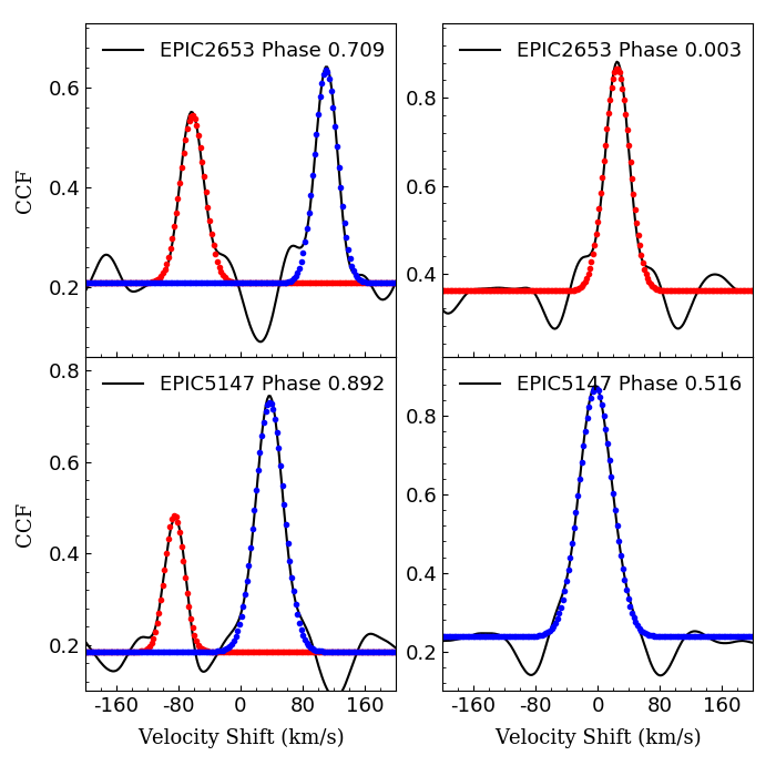
Figure 3: Some cross-correlation functions for EPIC2753 and EPIC5147 at phases close to quadratures and primary/secondary eclipses. The blue and red line are the fitted Gaussians for primary and secondary components, respectively.

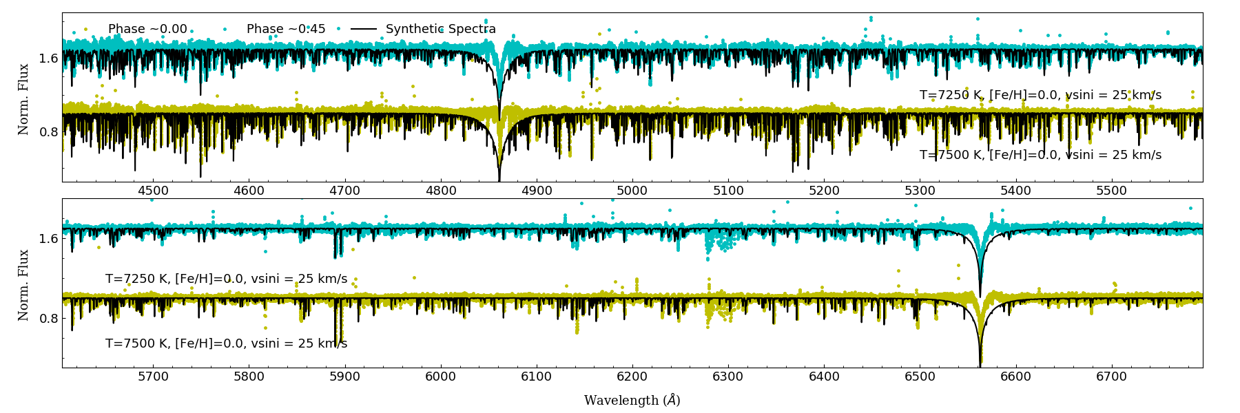
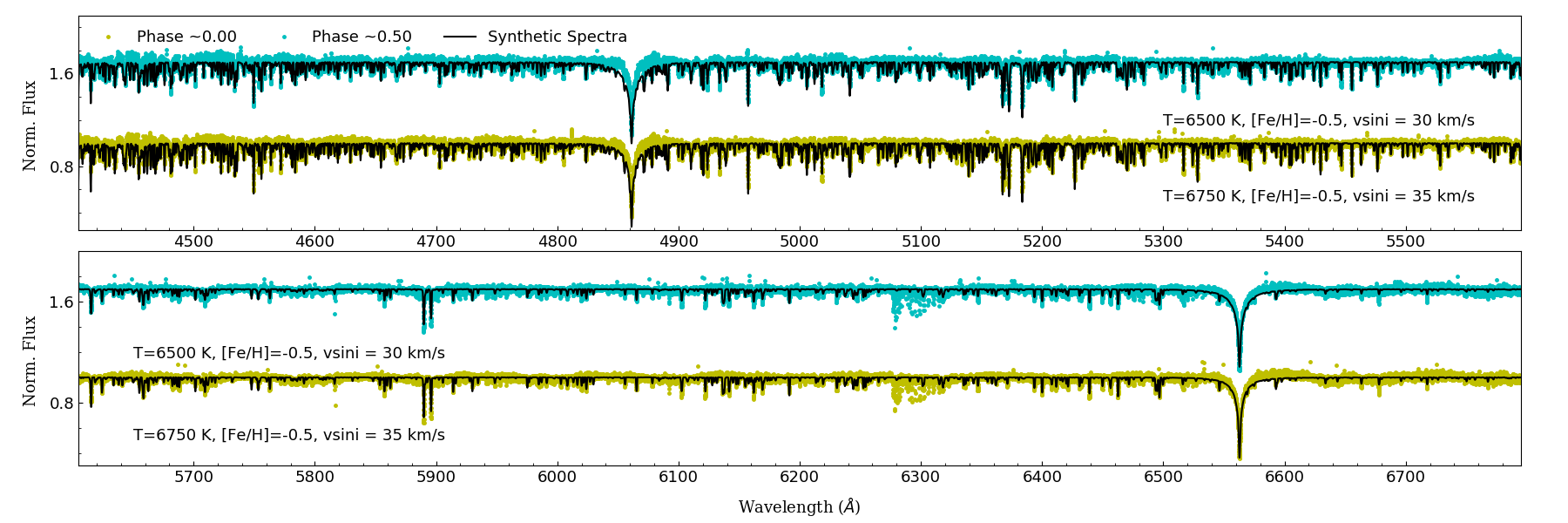
Figure 4: The observed HERMES spectra (in color) along with best fit synthetic spectra (in black) for EPIC2753 (upper panel) and EPIC5147 (lower panel) at an orbital phase around primary eclipse and secondary eclipse.

Table 8: The RV data for both the components of EPIC2753 and EPIC5147.

BJD	Phase	$RV_{1}$	Error	$RV_{2}$	Error
(+2450000)		km/sec	km/sec	km/sec
EPIC2753
8487.6401	0.709	+109.13	0.79	-064.69	1.68
8488.6142	0.890	+081.49	0.56	-035.52	1.41
8489.6271	0.078	-016.53	0.94	+069.25	1.55
8491.6412	0.451	-000.23	0.77	+051.64	1.26
8492.6147	0.632	+088.73	0.88	-042.45	1.01
8493.6189	0.818	+104.86	0.59	-059.57	1.08
8494.6118	0.003	—	—	+024.60	0.68
8495.6105	0.188	-056.23	0.84	+111.26	1.17
8496.6003	0.372	-037.78	0.68	+091.24	1.07
8521.5643	0.003	—	—	+024.84	0.67
EPIC5147
8487.6557	0.516	+003.30	0.60	—	—
8488.6281	0.784	+087.61	0.92	-100.11	3.03
8489.6410	0.064	-032.81	0.13	+039.50	3.49
8491.6550	0.620	+061.59	0.46	-069.14	0.75
8492.6396	0.892	+056.83	0.37	-064.12	0.87
8493.6318	0.166	-075.39	0.38	+090.25	0.31
8494.6292	0.441	-029.91	0.27	+036.19	5.53
8495.6281	0.717	+087.69	0.85	-099.88	4.72
8496.6132	0.989	—	—	+002.41	0.40
8520.5867	0.609	+057.10	0.51	-064.47	0.63
8520.5988	0.612	+058.38	0.50	-065.63	0.54
8522.5757	0.158	-072.99	0.67	+087.17	0.76
8524.5703	0.709	+086.42	0.58	-098.79	3.84
8525.5787	0.987	—	—	+003.10	0.53
8526.5397	0.252	-087.51	1.17	+103.53	4.86
8527.5523	0.532	+019.31	0.27	-018.70	3.70
8528.5736	0.814	+082.92	0.62	-093.67	4.19
8541.5097	0.386	-057.30	0.39	+068.36	1.54

5 Modeling

For photometric and radial velocity data modeling, the python-based modeling package PHOEBE 1.0 (PHysics Of Eclipsing BinariEs) is used (Prša & Zwitter, 2005). The software is based on the popular FORTRAN-based WD program (Wilson & Devinney, 1971). The graphical user interface (GUI) in PHOEBE is used for obtaining initial estimates of the parameters by viewing the synthetic fit at regular intervals after multiple iterations. The PHOEBE scripter is used to refine the parameters and determine the uncertainties in the parameters. The radial velocity (RV) and the photometric data can be analyzed together. The TOM at $0^{th}$ epoch and $P_{\rm orb}$ are used from section 3. The temperature estimates available in Gaia Collab. (2022) are used as the $T_{\rm eff}$ of the primary component for both the sources. For EPIC2753 and EPIC5147, the Gaia DR-3 $T_{\rm eff}$ are reported as 7416($\pm$12) and 6654($\pm$ 19), respectively. The $T_{\rm eff}$ are determined by General Stellar Parametrizer from Photometry (GSP-Phot) pipeline using low-resolution BP/RP spectra. GSP-Phot uses an Aeneas algorithm which employs MCMC to optimize the parameters. The components with $T_{\rm eff}$ below 7200 K are assumed to have a convective envelope. The surface albedo (A; fraction of light reflected by a star) and gravity brightening (g; variation in the pole to equator surface brightness of a star due to its rotation) for convective envelope stars are taken as 0.5 and 0.32, respectively. The surface albedo (A) and gravity brightening (g) for radiative envelope stars ($T_{\rm eff}>$ 7200 K) are taken as 1.0 and 1.0, respectively. The limb darkening coefficients are updated by the software after each iteration using the tables by van Hamme (1993). Known parameters such as HJD_o, the $P_{\rm orb}$  and the primary component’s effective temperature are fixed during analysis. During the first run, both the photometric and RV data are modeled using the PHOEBE GUI, to estimate the remaining free parameters. Based on the shape of LCs, the "Detached model" is used for both the systems. The semi-major axis (a; separation between EB components), center of mass velocity ($V_{\gamma}$; velocity of the center of mass of the EB system), mass ratio (q=$m_{2}/m_{1}$), inclination (i; angle between EB orbital plane and the sky plane), secondary component’s $T_{\rm eff}$, primary component passband luminosity ($l_{1}$; used to calculate the luminosity ratio for the components from input uncalibrated/calibrated LCs, not necessarily in standard units), primary and secondary component surface potential ($\Omega_{1/2}$; dimensionless potential or the modified Kopal potential) are set free. The eccentricity of both systems are taken as 0. The fitted LC and RV curves for each system are shown in Fig. 5, Fig. 6, Fig. 7, and Fig. 8.

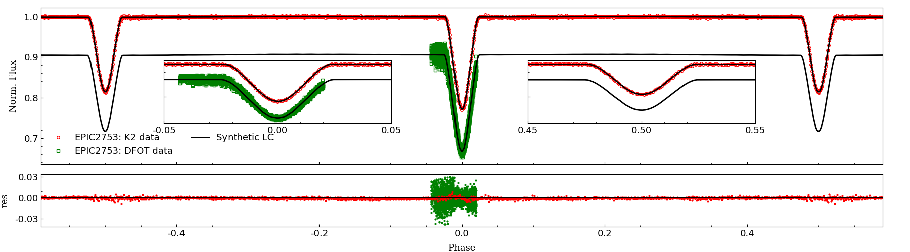
Figure 5: Combined K2 data from different campaigns and DFOT $R_{c}$-band data along with synthetic LCs (continuous line) for EPIC2753.

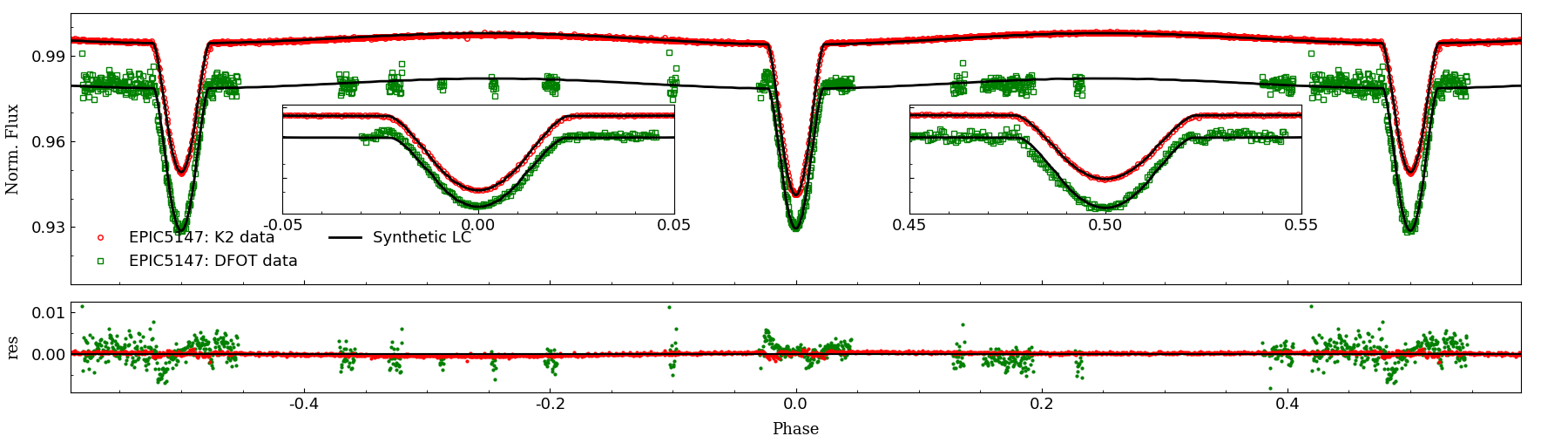
Figure 6: Same as Fig. 5 but for EPIC5147.

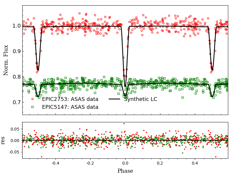
Figure 7: ASAS-3 observations for EPIC2753 and EPIC5147 with synthetic LCs.

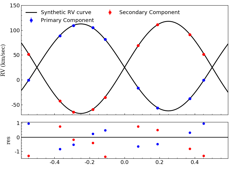
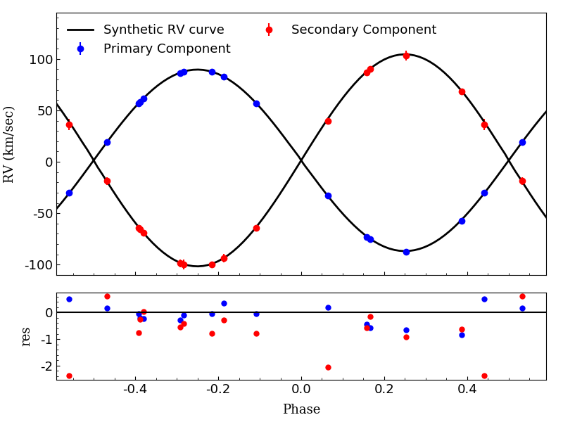
Figure 8: The RV variation for primary and secondary components of EPIC2753 (upper panel) and EPIC5147 (lower panel) with the model fit.

In the K2 data set, the brightness of system EPIC5147 is found to be slightly different at phases 0.25 and -0.25. The system has slightly high brightness at phase 0.25 as compared to phase -0.25. For this asymmetry of LC, one dark spot at primary and one at secondary are placed. Different positions and parameters of spot are compared on the basis of sum of square of residuals (SSR) to select the final solution. The position of a spot on stellar surface is defined by spot colatitude and spot longitude. Spot colatitude is the angular distance of the spot as measured from the North pole of the star (0 to 180^∘) while spot longitude is the angular distance of the spot as measured from the direction of the companion in counter clockwise direction (0 to 360^∘). The radius of the spot (in degrees) specifies spot size and temperature ratio is defined as the ratio of the spot temperature with respect to local temperature of photosphere. Fig. 9 shows the residuals of fit with and without the use of spots in the model. The spot parameters are determined as colatitude: 90^∘ (fixed), longitude: 270^∘ ($\pm$5), spot radius: 25^∘ ($\pm$5), and temperature ratio ($T_{spot}/T_{star}$): 0.998 for spot on primary component. For spot on secondary component, colatitude: 90^∘ (fixed), longitude: 275^∘ ($\pm$5), spot radius: 30^∘($\pm$5), and temperature ratio ($T_{spot}/T_{star}$): 0.997. Although the level of asymmetry is very small and actual cause of the uneven brightness is unclear, the inclusion of the spots during the modeling resulted in a slightly better fit. The position of spot is shown in Fig. 10. Both the components are scaled according to a normalized semi-major axis (a).

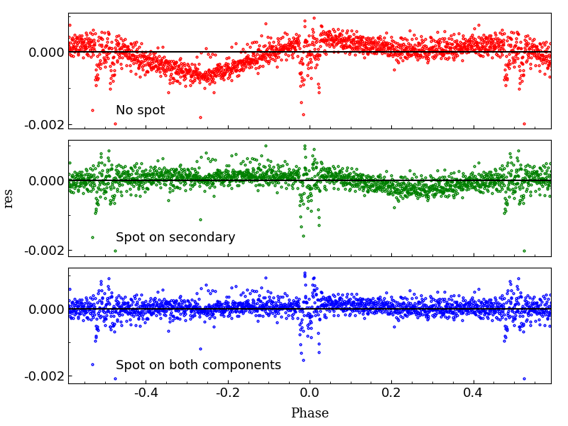
Figure 9: Change in the fit residuals for EPIC5147 after including spots.

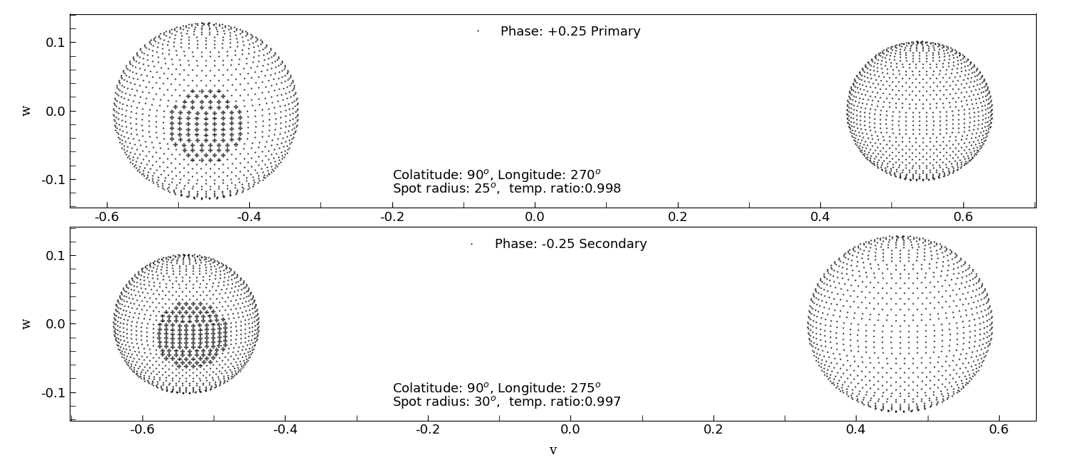
Figure 10: Position of spots on primary (upper panel) and secondary (lower panel) components of the system EPIC5147 as seen during phases 0.25 and -0.25.

The errors given by PHOEBE GUI are fitting errors, which are probably an underestimation of the true errors. To estimate the errors more robustly, we use the Markov Chain Monte Carlo (MCMC) method. A Python script is developed by Prša & Zwitter (2005) which allows the user to apply the EMCEE code (Foreman-Mackey et al., 2013) with the PHOEBE scripts. The EMCEE code is a Python implementation of Goodman $\&$ Weare’s Affine Invariant Markov chain Monte Carlo (MCMC) Ensemble sampler (Goodman & Weare, 2010). During the MCMC run, the semi-major axis (a), center of mass velocity ($V_{\gamma}$), mass ratio (q), inclination (i), secondary component’s $T_{\rm eff}$ and primary/secondary component surface potential ($\Omega_{1,2}$) are set as free parameters. Appropriate lower and upper limits are used for these free parameters. A combination of 125 walkers and 8,000 iterations is used for MCMC runs. First 1,00,000 iterations are discarded from all 10,00,000 (125$\times$8,000) iterations as MCMC burn-in period. The corner plots for the MCMC runs are given in Figure 11 for both sources. The quantities at the top of subplots are 1, 50, and 99 percentiles for each distribution. The standard deviation for the MCMC distribution of each parameter is reported as the uncertainty. Table 9 lists the values for determined parameters from the best fitted model and their MCMC derived uncertainties. The quantities $r_{1,2}$ in the Table 9 are the component radii normalized to the semi-major axis or simply the dimensionless/normalized radii. PHOEBE calculates $r_{1,2}$ using the $\Omega_{1/2}$. Note that the peaks of the MCMC distributions shown in Figure 11 are slightly different from the best model parameters mentioned in Table 9 as distributions are represented by histograms with some bin width for different parameters.

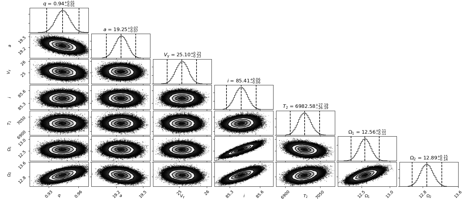
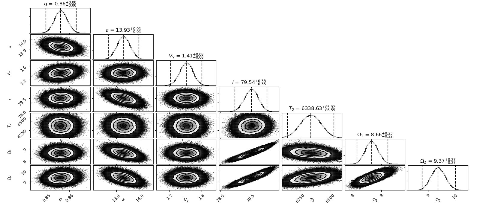
Figure 11: Corner plots MCMC distributions for EPIC2753 (lower panel) and EPIC5147 (upper panel). The vertical dashed lines represent the 1, 50 and 99 % quantiles of distribution.

Table 9: The combined LC and RV solutions for both the systems. The ’*’ indicates the errors are determined using MCMC distribution.

Parameters	Kepler/K2	Kepler/K2
	EPIC2753	EPIC5147
a ($R_{\odot}$)	19.26(0.07)*	13.92(0.03)*
$V_{\gamma}$ (km/s)	25.1(0.2)*	1.41(0.08)*
q	0.942(0.007)*	0.856(0.003)*
i (∘)	85.53(0.05)*	79.71(0.34)*
$T_{\rm eff,2}$	6981(28)*	6318(85)*
$l_{1}$	7.414(0.008)	8.377(0.007)
$l_{2}$	5.145	4.154
$\Omega_{1}$	13.56(0.11)	8.61(0.23)
$\Omega_{2}$	12.88(0.15)	9.49(0.27)
$r_{1}$ (a)	0.0861(0.0009)	0.1292(0.0037)
$r_{2}$ (a)	0.0797(0.0010)	0.1021(0.0033)

5.1 Absolute Parameters

The orbital solutions derived via model fitting are used to estimate the fundamental parameters such as radius (to make things clear for coming sections, the parameter "radius or $R_{1,2}$" is used to represent the component radius in solar radius units and "normalized radius or $r_{1,2}$" to represent the radius in semi-major axis units), mass and luminosity of individual components. The RV modeling give semi-major axis (a) and with the help of known value of $P_{\rm orb}$, total mass of the system ($M_{T}=M_{1}+M_{2}$) is calculated. The semi-major axis normalized radii for components are converted to actual radii in solar radius units using the semi-major axis. The mass-ratio q is used to determine the masses of individual components. The radius of each component is derived from model fitting and the temperatures of the individual components are used to estimate the luminosity of the individual components. The total luminosity of the system can be converted to the bolometric luminosity and absolute magnitudes with the help of appropriate bolometric corrections. The distance modulus is related to the absolute and apparent magnitude which give the distance of the system. The parameters and uncertainties are determined using the FORTRAN code JKTABSDIM (Southworth et al., 2005). JKTABSDIM uses bolometric correction tables by Girardi et al. (2002) for estimating absolute magnitudes. The absolute parameters are listed in the Table 10. The distance estimates from code JKTABSDIM given in Table 10 make use of the surface brightness relations by Kervella et al. (2004).

5.2 Evolutionary Status

To probe the stellar evolution, isochrones and stellar evolutionary tracks are generated using MESA Isochrones $\&$ Stellar Tracks (MIST, Paxton et al. 2011; Choi et al. 2016; Dotter 2016). While generating the stellar evolutionary tracks, the initial masses close to the calculated masses are chosen. For isochrones, the log(Age[Yr]) is varied from 8.00 to 10.00 in steps of 0.05. The metallicity [Fe/H]=0.2 is used for stellar evolution tracks/isochrones. Fig. 12 shows the MIST evolutionary tracks/isochrones with the EPIC2753 and EPIC5147 components. Only the main sequence part of the evolutionary tracks and isochrones is shown in Fig. 12. Different colors in stellar evolutionary tracks (continuous lines) and isochrones (dashed lines) represents different initial masses and ages, respectively. The components of EPIC2753 lie close to the isochrones with log(Age) = 8.20 to 8.35 (100 Myr-224 Myr). The secondary component of EPIC2753 is found to have slightly low luminosity and radius as expected from the used isochrones. The components of EPIC5147 lies close to the isochrones with log(Age) = 9.20 to 9.40 (1.6-2.5 Gyr).

Table 10: The absolute parameters derived for the system in the present study.

Parameters	Kepler/K2	Kepler/K2
	EPIC2753	EPIC5147
d (pc)	238(4)	199(5)
$M_{1}$ ($M_{\odot}$)	1.69(0.02)	1.48(0.01)
$M_{2}$ ($M_{\odot}$)	1.59(0.02)	1.27(0.01)
$R_{1}$ ($R_{\odot}$)	1.66(0.02)	1.80(0.05)
$R_{2}$ ($R_{\odot}$)	1.53(0.02)	1.42(0.05)
$L_{1}$ ($L_{\odot}$)	7.50(0.17)	5.72(0.33)
$L_{2}$ ($L_{\odot}$)	5.05(0.15)	2.91(0.24)

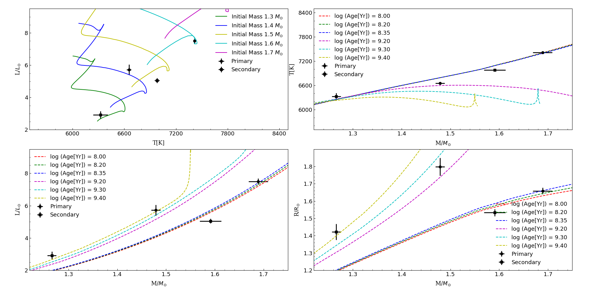
Figure 12: The upper left plot shows the position of components along evolutionary tracks with different initial masses. The other plots show position of targets in M-T, M-L and M-R plane along with different isochrones from MIST.

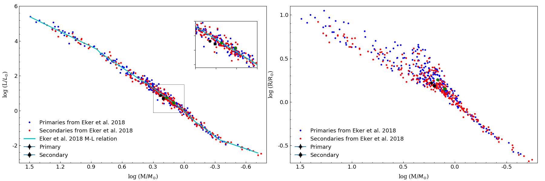
Figure 13: The component parameters along with other well characterized EBs. EPIC2753 and EPIC5147 components are shown in green and black color, respectively.

6 Results and Discussion

Double-lined detached EBs are crucial to test the models of stellar structure and evolution. The multiple campaign photometric data from K2 is analyzed with the RV data for two eclipsing binary candidates to derive accurate physical parameters. Sources are also observed using the 1.3-m DFOT, Nainital and ASAS-3 survey. The systems are mentioned in some surveys but this work is the first one where a complete characterization of the systems is done. The TOMs are determined using data sets from multiple K2 campaigns with a time basis of almost 3.2 years. The $P_{\rm orb}$ is found to be constant over a period of 3.2 years for both systems. Updated linear ephemeris are derived using these data. The $P_{\rm orb}$ is mentioned as 1.8112662 days in Barros et al. (2016) for EPIC5147 while we derived $P_{\rm orb}$ as 3.6215398 days. The results of Barros et al. (2016) are solely based on K2 C05 observations while the present work gives a more reliable ephemeris for EPIC5147 by including C16, C18 observations. Although present analysis does not highlight any variation in period of these systems, it is impossible to completely discard the possibility of period variation on the basis of a time span as short as 3.2 years.

The masses and radii of the components of EPIC2753 are derived as $M_{1,2}$ = 1.69(0.02), 1.59(0.02) $M_{\odot}$ and $R_{1,2}$ = 1.66(0.02), 1.53(0.02) $R_{\odot}$. Similarly, the masses and radii of the components of EPIC5147 are derived as $M_{1,2}$ = 1.48(0.01), 1.27(0.01) $M_{\odot}$ and $R_{1,2}$ = 1.80(0.05), 1.42(0.05) $R_{\odot}$.

Eker et al. (2018) derived mass-luminosity and mass-radius relations using 509 well-studied main-sequence stars in detached eclipsing binary systems. The mass-luminosity data are represented in the form of six-piece classical mass-luminosity relation for six different mass ranges. The mass-radius relation is derived for stellar masses ranging from 0.179 to 1.5 $M_{\odot}$. For EPIC2753 the component luminosities are derived as $L_{1,2}$ = 9.88(0.79) and 7.64(0.65) $L_{\odot}$ using the mass-luminosity relation for intermediate mass stars. For EPIC5147 and $L_{1,2}$ are calculated as 5.56(0.34) $L_{\odot}$ and 2.84(0.16) $L_{\odot}$ from mass-luminosity relation. Similarly, use of mass-radius relation estimated the primary and secondary component radius $R_{1,2}$ as 1.74(0.59) $R_{\odot}$ and 1.39(0.55) $R_{\odot}$ for EPIC5147. For EPIC5147, the results by these relations are same as our estimates within error limits but for EPIC2753, the estimated luminosities are higher than expected values. One reason for this deviation in the results can be the non-homogeneous nature of the sample used by Eker et al. (2018). A large fraction of the stars in the studied sample consists of main sequence stars from the solar neighborhood disc which are mostly metal rich. The empirical relations by Eker et al. (2018) do not involve the effect of metallicity. Only a limited number of stars in the sample have trustworthy metallicity estimates. The mass-radius and mass-luminosity relations can be different for samples with different ages and metallicity. Fernandes et al. (2021) derived mass-radius and mass-luminosity relations including the effects of age and metallicity but the results are based on a small sample of 56 stars. The study of their effect on mass-luminosity and mass-radius relations need more large sample of stars with reliable age and metallicity measurements. Figure 13 shows the component parameters of studied EBs with other EB components used by Eker et al. (2018) to derive the relations. The continuous line in the left panel of Figure 13 represents the six-piece M-L relation by Eker et al. (2018).

The distances are derived as 238 (4) and 199 (5) pc for EPIC2753 and EPIC5147, respectively. The distances for these sources are mentioned as $\sim$ 248 (1) pc (for EPIC2753) and $\sim$ 200 (2) pc (for EPIC5147) in Gaia Collab. (2021) catalog which are close to our estimates. The evolution status of the systems are investigated using the MESA evolutionary tracks and isochrones. The comparison of EPIC2753 components with different isochrones shows that the age of the system is around 100-224 Myr. The age of system EPIC5147 is determined as 1.6-2.5 Gyr on the basis of isochrones. Other constraints such as accurate $\log g$ and [Fe/H], can further refine the age estimates.

Data Availability

The data supporting the results of this study are available from the corresponding author on reasonable request.

References

- Alpaslan (2009) Alpaslan M., 2009, arXiv e-prints, p. arXiv:0912.4755
- Barros et al. (2016) Barros S. C. C., Demangeon O., Deleuil M., 2016, A&A, 594, A100
- Bate et al. (2002) Bate M. R., Bonnell I. A., Bromm V., 2002, MNRAS, 336, 705
- Bodenheimer (2011) Bodenheimer P. H., 2011, Principles of Star Formation, doi:10.1007/978-3-642-15063-0.
- Borucki et al. (2010) Borucki W. J., et al., 2010, Science, 327, 977
- Bourges et al. (2017) Bourges L., Mella G., Lafrasse S., Duvert G., Chelli A., Le Bouquin J. B., Delfosse X., Chesneau O., 2017, VizieR Online Data Catalog, p. II/346
- Castelli & Kurucz (2003) Castelli F., Kurucz R. L., 2003, in Piskunov N., Weiss W. W., Gray D. F., eds, Symposium of the International Astronomical Union Vol. 210, Modelling of Stellar Atmospheres. p. A20 (arXiv:astro-ph/0405087)
- Choi et al. (2016) Choi J., Dotter A., Conroy C., Cantiello M., Paxton B., Johnson B. D., 2016, ApJ, 823, 102
- Collins et al. (2017) Collins K. A., Kielkopf J. F., Stassun K. G., Hessman F. V., 2017, AJ, 153, 77
- Cutri et al. (2003) Cutri R. M., et al., 2003, VizieR Online Data Catalog, p. II/246
- Cutri et al. (2012) Cutri R. M., et al., 2012, Explanatory Supplement to the WISE All-Sky Data Release Products, Explanatory Supplement to the WISE All-Sky Data Release Products
- Dotter (2016) Dotter A., 2016, ApJS, 222, 8
- Eker et al. (2018) Eker Z., et al., 2018, MNRAS, 479, 5491
- Fabian et al. (1975) Fabian A. C., Pringle J. E., Rees M. J., 1975, MNRAS, 172, 15
- Fernandes et al. (2021) Fernandes J., Gafeira R., Andersen J., 2021, A&A, 647, A90
- Foreman-Mackey et al. (2013) Foreman-Mackey D., Hogg D. W., Lang D., Goodman J., 2013, PASP, 125, 306
- Gaia Collab. (2021) Gaia Collab. 2021, A&A, 649, A1
- Gaia Collab. (2022) Gaia Collab. 2022, VizieR Online Data Catalog, p. I/355
- Girardi et al. (2002) Girardi L., Bertelli G., Bressan A., Chiosi C., Groenewegen M. A. T., Marigo P., Salasnich B., Weiss A., 2002, A&A, 391, 195
- Goodman & Weare (2010) Goodman J., Weare J., 2010, Communications in Applied Mathematics and Computational Science, 5, 65
- Goodwin et al. (2004) Goodwin S. P., Whitworth A. P., Ward-Thompson D., 2004, A&A, 414, 633
- Gray (1999) Gray R. O., 1999, SPECTRUM: A stellar spectral synthesis program, Astrophysics Source Code Library, record ascl:9910.002 (ascl:9910.002)
- Higl & Weiss (2017) Higl J., Weiss A., 2017, A&A, 608, A62
- Høg et al. (2000) Høg E., et al., 2000, A&A, 355, L27
- Hurley et al. (2002) Hurley J. R., Tout C. A., Pols O. R., 2002, MNRAS, 329, 897
- Joshi et al. (2019) Joshi Y. C., De Cat P., Panchal A., Goswami A., Lampens P., Vermeylen L., Maurya J., 2019, Bulletin de la Societe Royale des Sciences de Liege, 88, 82
- Kervella et al. (2004) Kervella P., Thévenin F., Di Folco E., Ségransan D., 2004, A&A, 426, 297
- Lenz & Breger (2005) Lenz P., Breger M., 2005, Communications in Asteroseismology, 146, 53
- Luger et al. (2016) Luger R., Agol E., Kruse E., Barnes R., Becker A., Foreman-Mackey D., Deming D., 2016, AJ, 152, 100
- Moe & Di Stefano (2017) Moe M., Di Stefano R., 2017, ApJS, 230, 15
- Okamoto & Sato (1970) Okamoto I., Sato K., 1970, PASJ, 22, 317
- Paxton et al. (2011) Paxton B., Bildsten L., Dotter A., Herwig F., Lesaffre P., Timmes F., 2011, ApJS, 192, 3
- Pojmański (2001) Pojmański G., 2001, in Paczynski B., Chen W.-P., Lemme C., eds, Astronomical Society of the Pacific Conference Series Vol. 246, IAU Colloq. 183: Small Telescope Astronomy on Global Scales. p. 53
- Prša & Zwitter (2005) Prša A., Zwitter T., 2005, ApJ, 628, 426
- Raskin et al. (2011) Raskin G., et al., 2011, A&A, 526, A69
- Ricker et al. (2015) Ricker G. R., et al., 2015, Journal of Astronomical Telescopes, Instruments, and Systems, 1, 014003
- Schlafly & Finkbeiner (2011) Schlafly E. F., Finkbeiner D. P., 2011, ApJ, 737, 103
- Southworth et al. (2005) Southworth J., Maxted P. F. L., Smalley B., 2005, A&A, 429, 645
- Street et al. (2003) Street R. A., et al., 2003, in Deming D., Seager S., eds, Astronomical Society of the Pacific Conference Series Vol. 294, Scientific Frontiers in Research on Extrasolar Planets. pp 405–408 (arXiv:astro-ph/0208233)
- Tokovinin & Moe (2020) Tokovinin A., Moe M., 2020, MNRAS, 491, 5158
- Tonry & Davis (1979) Tonry J., Davis M., 1979, AJ, 84, 1511
- Torres et al. (2010) Torres G., Andersen J., Giménez A., 2010, A&ARv, 18, 67
- Wilson & Devinney (1971) Wilson R. E., Devinney E. J., 1971, ApJ, 166, 605
- Wraight et al. (2011) Wraight K. T., White G. J., Bewsher D., Norton A. J., 2011, MNRAS, 416, 2477
- Wraight et al. (2012) Wraight K. T., Fossati L., White G. J., Norton A. J., Bewsher D., 2012, MNRAS, 427, 2298
- van Hamme (1993) van Hamme W., 1993, AJ, 106, 2096