cortheo \newaliascntproptheo \newaliascntlemmatheo \aliascntresetthecor \aliascntresettheprop \aliascntresetthelemma \newaliascntdefitheo \newaliascntassumtheo \newaliascntassumstheo \newaliascntprobtheo \aliascntresetthedefi \aliascntresettheassum \aliascntresettheassums \aliascntresettheprob \newaliascntremstheo \newaliascntremtheo \newaliascntexatheo \newaliascntexstheo \aliascntresettherems \aliascntresettherem \aliascntresettheexa \aliascntresettheexs
Pointwise eigenvector estimates by landscape functions:
some variations on the Filoche–Mayboroda–van den Berg bound
Abstract.
Landscape functions are a popular tool used to provide upper bounds for eigenvectors of Schrödinger operators on domains. We review some known results obtained in the last ten years, unify several approaches used to achieve such bounds, and extend their scope to a large class of linear and nonlinear operators. We also use landscape functions to derive lower estimates on the principal eigenvalue – much in the spirit of earlier results by Donsker–Varadhan and Bañuelos–Carrol – as well as upper bounds on heat kernels. Our methods solely rely on order properties of operators: we devote special attention to the case where the relevant operators enjoy various forms of elliptic or parabolic maximum principles. Additionally, we illustrate our findings with several examples, including -Laplacians on domains and graphs as well as Schrödinger operators with magnetic and electric potential, also by means of elementary numerical experiments.
Key words and phrases:
Landscape functions; positive -semigroups; -Laplacians; Magnetic Schrödinger operators2010 Mathematics Subject Classification:
Primary 34B45, 35P15, 34L15, 35P30; Secondary 46B42, 47B65The author was partially supported by the Deutsche Forschungsgemeinschaft (Grant 397230547).
1. Introduction
Several authors have pursued in the last ten years the task of deriving pointwise bounds of the form
| (1.1) |
on all eigenpairs of suitable differential operators in terms of one auxiliary function : such satisfying (1.1) or, more generally,
for some , have been often called landscape functions since [28]. In the case of Schrödinger operators, with and with Dirichlet conditions on the boundary of a bounded , Filoche and Mayboroda have proved in [28] that a possible landscape function is given by the unique solution of
| (1.2) |
the same estimate has been independently observed in [8] for . Observe that the Schrödinger operator satisfies a weak maximum principle, that is, is a positive operator: hence, the solution of (1.2) is indeed a positive function. Such is sometimes called the torsion function of (with respect to ) and has since [62] been the subject of many investigations.
In the case of such Schrödinger operators, a common interpretation of (1.1) is that any eigenfunction for the eigenvalue can only have peaks (“localize”) in the set . Because similar localization properties hold for the potential wells (see, e.g., [40, Theorems 3.4 and 3.10]), it is tempting to interpret as a proxy for the potential . The fact that is typically smoother than and even more effective at predicting localization of eigenfunctions justifies the attention devoted to (1.1) in the last years.
To fix the ideas at the core of the theory of landscape functions, let us present its fundamental theorem in a general form that holds for operators on a Lebesgue space that have dominated inverse, i.e., such that
for some bounded linear (and necessarily positive) operator on .
Theorem 1.1.
Let be a finite measure space, and let be an invertible closed linear operator on with dominated inverse. If is an eigenpair of such that , then
| (1.3) |
By (1.3), any eigenfunction of for the eigenvalue can only localize in the set . Theorem 1.1 was proved by van den Berg in [8, Theorem 5] (for the free Laplacian) and by Filoche and Mayboroda in [29, Proposition 0.1] (for Schrödinger operators with positive potential) using – beside the maximum principle – self-adjointness, resolvent compactness, and the existence of a positive Green function ([28]) or a positive heat kernel ([8]); but their proofs do not actually depend on whether or not. Indeed, it was observed by Steinerberger in [64, page 2903] (and, in a slightly different context, already in the proof of [53, Lemma 3]) that these assumptions can be removed and the proof boils down to a one-liner that can be performed under the sole assumption that the relevant operator has dominated inverse.
Proof of Theorem 1.1.
Let to see
| (1.4) |
This works upon choosing whenever has positive inverse (the case treated in [8, 28, 64]) and in fact even for general dominating operators : the latter case has been discussed in the settings of operators whose inverse has a (not necessarily positive!) absolutely integrable kernel in [29], and of matrices in [48]; in the latter case, lower bounds for eigenfunctions in their localization regions are discussed in [52].
Being interested in pointwise bounds, it appears natural to lift the problem and regard (1.1) as an inequality between “absolute value” of vectors, just like in (1.4). In this note we will extend the ideas in [8, 28] to the much more general setting of operators on Banach lattices: a canonical setting where absolute values of vectors are well-defined. This includes elliptic operators on Lebesgue spaces or spaces of continuous functions vanishing at infinity over a locally compact metric space, but also more exotic objects, like pseudo-differential operators (including fractional Laplacians or Dirichlet-to-Neumann operators), infinite dimensional Ornstein–Uhlenbeck processes, or Lindbladian generators on spaces of Schatten–von Neumann operators over a Hilbert space.
Theorem 1.1 especially applies to large classes of (not necessarily self-adjoint) uniformly elliptic and even degenerate second order operators satisfying a weak maximum principle, and in particular to Schrödinger operators with a positive (possibly singular) potential and/or with boundary conditions on bounded open domains of or on suitable subset of compact manifolds – this is the setting discussed in [28, 3] – but also on finite metric [38, 57] or combinatorial graphs [30]: in these settings, again, is the usual choice.
The scope of this note is twofold. On the one hand, we borrow different Ansätze proposed by several authors to sharpen the original bound by Filoche–Mayboroda–van den Berg and unify them: we can thus present, in an abstract functional analytical framework, a minimal set of assumptions that allow to re-derive numerous landscape-functions-based estimates for differential and difference operators that have been presented by different authors over the last ten years. On the other hand, we are going to elaborate on Theorem 1.1 in three different directions.
Firstly, we extend in Section 2 the scope of the theory of landscape functions to nonlinear homogeneous operators, whose spectral theory relies on well-known variational tools, cf. [32, Chapter III].
Secondly, we discuss in Section 3 two different linear setups to which the ideas of van den Berg and Filoche–Mayboroda can be extended: we consider the cases of landscape functions for the eigenvectors of operators satisfying some very weak form of a maximum principle (namely, existence of a positive operator that dominates the inverse), and of integral operators (in the sense of [2, Definition 1.1]), in Section 3.1 and 3.2, respectively. We present sharper versions of Theorem 1.1 and argue that the key argument in their proof is the assumption that generates a positive semigroup, or even a semigroup that is merely dominated by a positive one. In passing, we also complement (1.1) with a similar upper estimate in terms of a parabolic landscape function: this corresponds to replacing the Green function by the heat kernel in the estimates in [8, 28]; in the case of Schrödinger operators, this idea has already been explored in [41, Theorem 2 and Corollary].
Thirdly, we show in Section 4 that landscape function methods can be adapted to derive lower bounds on the principal eigenvalue of the relevant (linear or nonlinear) operators: we here elaborate on an old idea by Donsker–Varadhan [24, 25] (as paraphrased e.g. in [13, Lemma 2.1]), later rediscovered e.g. in [5] and, for nonlinear homogeneous operators, in [33]: observe that these results predate the development of the theory of landscape functions. We describe a whole class of landscape functions – including the torsion function – and minimize their gauge norm within to derive an improved lower bound.
We conclude our note reviewing in Section 5 several classes of operators to which our results can be applied: In Section 5.1 we will show how our techniques can be used to derive rather sharp estimates on the ground state of a self-adjoint operator; we will treat a nonlinear counterpart in Section 5.2 and show that our methods can be seen as a relaxation of the search for the Cheeger constant. Finally, in Section 5.3 we present an application to a family of operators that may fail to have positive inverse: we derive from the Kato–Simon diamagnetic inequality a new proof of an estimate recently obtained in [41] under somewhat stronger assumptions.
In the following we will assume that the reader is familiar with the theory of Banach lattices and of linear operators thereon, as presented e.g. in [63, 58]: among other things, we will throughout use properties of positive linear (and order preserving nonlinear) operators, and sometimes assume that operators are dominated by other operators, or that they even have a modulus operator.
An especially important notion is the following: Given a Banach lattice with positive cone and some , the principal ideal generated by is the vector space
which by the results in [63, Section II.7] becomes a Banach lattice when endowed with the gauge norm
| (1.5) |
The easiest possible – and perhaps canonical – example is that of Lebesgue spaces over a finite measure space . Then is for each a Banach lattice (with respect to the pointwise defined order relation between functions); upon taking , one e.g. finds .
More generally, because is in fact an AM space – indeed, it is isometrically Banach lattice isomorphic to for some compact Hausdorff space (with ) – the infimum in (1.5) is attained, i.e., for all . We will also make use of ideas from the theory of eventually positive -semigroups, see [35] for a gentle introduction.
2. Eigenvector bounds by landscape functions: The nonlinear case
The proof of Theorem 1.1 relies solely on the homogeneity of , rather than on the full linearity of . We will elaborate on this idea in this section, often making good use of the properties of (nonlinear) maximal monotone operators: two standard references are [14] for the general theory of such operators, and [7, 17] for their interplay with the theory of Banach lattices.
Given some , a vector space and a (possibly nonlinear and multi-valued) operator on , we follow [15] and say that is -homogeneous if its domain is a cone and
| (2.1) |
A direct computation yields the following.
Lemma 2.1.
Let be a -homogeneous operator on a vector space , for some . Then its inverse – if it exists – is -homogeneous, i.e., it satisfies
| (2.2) |
Example \theexa.
(1) Linear operators are -homogeneous, and so is for all , the normalized -Laplacian , see [44] and references therein, defined by
as well as
(2) A subdifferential of a convex, proper, lower-semicontinuous functional on a Hilbert space (see [14, Exemples 2.1.4 and 2.3.4]) is a -homogeneous operator whenever is absolutely -homogeneous, i.e., provided
for any . Thus, examples of absolutely -homogeneous operators are given by the (standard) -Laplacians on open bounded domains of (in particular, with homogeneous Dirichlet or Neumann conditions, but also with suitable Robin-type conditions [47]), on combinatorial [55] or metric graphs [22]; by Finsler -Laplacians [27]; by non-local -Laplacians [1, Chapter 6]; by -Dirichlet-to-Neumann operators [16]; by fractional -Laplacians [23]; or by subdifferential of general -Cheeger energies on general metric measure spaces recently introduced in [37]. Operators associated with porous medium equations in are -homogeneous, too, for suitable .
Recall that a single-valued operator on a vector lattice is said to be order preserving if
and to dominate another single-valued operator on if
The following property is well-known in the case of linear operators, see the proof of [60, Proposition 2.20].
Lemma 2.2.
Let be a vector lattice and let be a (possibly multi-valued) invertible -homogeneous operator for some . If is single-valued and order preserving, then it dominates itself. In particular, for all .
Proof.
Because , we deduce from (2.2) that . ∎
If, for some , is a (possibly multi-valued) -homogeneous operator with domain and there exists and such that
| (2.3) |
then is said to be an eigenvector of for the eigenvalue or, shortly, we call an eigenpair of .
Proposition \theprop.
Let be a real Banach lattice, and let . Let , and let be (possibly multi-valued) maximal monotone, -homogeneous and invertible operators on , and such that is order preserving and dominates . Then for any eigenpair of such that there holds
| (2.4) |
If has order preserving inverse, then we can take in (2.4).
Proof.
Applying the single-valued operator to both sides of (2.3) yields
Now we apply Lemma 2.1 and proceed like in the proof of Theorem 1.1 to deduce the claim, using the fact that is an -space and, hence, . The second assertion follows from Lemma 2.2. ∎
Inspired by the general setting proposed in [59], we may also consider eigenpairs of -homogeneous operators with respect to another (single-valued!) -homogeneous operator : by this we mean that
The case discussed in the first part of this section corresponds to the choice
but if is a finite measure space and we may also let
or, more generally,
We can hence obtain a generalization of Section 2: the proof is identical and we omit it.
Corollary \thecor.
Let be a real Banach lattice, and let . Let , and let be (possibly multi-valued) maximal monotone, -homogeneous and invertible operators on , and such that is order preserving and dominates . Then for any eigenpair of with respect to a -homogeneous operator on we have
3. Eigenvector bounds by landscape functions: The linear case
3.1. Estimates by order properties
For the sake of later reference, let us first state a more general version of Theorem 1.1 that applies to operators that are not invertible: its proof is an obvious modification of (1.4).
Theorem 3.1.
Let be a Banach lattice, and let . Let be a closed linear operator on a Banach lattice such that is invertible and is dominated by some bounded linear operator . If is an eigenpair of such that , then
| (3.1) |
Clearly, we may take if has positive inverse.
Remark \therem.
There is a curious counterpart of the concept of landscape function in the classical Birman–Schwinger theory: Given a potential , a simple manipulation shows that is an eigenpair for the Schrödinger operator if and only if
| (3.2) |
i.e., if and only if is an eigenpair for the operator , where formally . Birman and Schwinger, and many authors after them elaborated on this observation to find spectral correspondences between and : see, e.g., [50, Chapter 4] for applications in modern mathematical physics.
However, inspired by (3.2) we can also find a new landscape function, hence deduce a new pointwise eigenvector bound: If , then by the maximum principle is a positive operator and (3.2) yields
| (3.3) |
to be compared with
| (3.4) |
from Theorem 3.1: the relative size of will decide which estimate is sharper.
(It should be appreciated that, in view of the Kato–Simon diamagnetic inequality, one also has the domination property for any magnetic Laplacian (under very mild integrability assumptions on , see [43, 54]) and, hence, (3.3) and (3.4) also hold for all eigenpairs of . We will elaborate on this in Section 5.3.)
Let us now present two further classes of landscape-type functions for possibly non-invertible operators. The first one is related to the anti-maximum principle, which has been studied for numerous linear and nonlinear operators since [18]: roughly speaking, validity of a maximum/anti-maximum principle results in a sudden “change of sign” (from order preservation to order reversal) of an operator’s resolvents across the bottom of its spectrum. The second one replaces the order properties of resolvents by those of -semigroups: we refer to [20] for the terminology. Here and in the following, we denote by the spectral bound of an operator .
Proposition \theprop.
Let be a closed linear operator on a complex Banach lattice , and let .
Then the following assertions hold for each eigenpair of such that .
-
(1)
Let be an eigenvalue and a pole of the resolvent , and let the corresponding eigenprojector be strongly positive with respect to . If is densely defined, then both
(3.5) and
(3.6) hold for all sufficiently small.
-
(2)
If generates a -semigroup that is individually eventually strongly positive with respect to , then there is such that
(3.7)
This suggests that is a landscape-like function: we will refer to it as a parabolic landscape function. If is a semigroup generator, and if is individually eventually strongly positive with respect to , then the condition that be strongly positive with respect to can be reformulated in terms of smoothing properties of , see [20, Theorem 5.2 and Corollary 5.3].
Proof.
(1) We apply [20, Theorem 4.4] and deduce that is a strongly positive (resp., strongly negative) operator for all in a sufficiently small (depending on ) left (resp., right) neighbourhood of . In particular, the estimates
| (3.8) |
and
| (3.9) |
hold for some and all small enough. In either estimate, the former inequality holds because dominates (resp., anti-dominates) itself, while the latter follows from the inequality .
(2) By the Spectral Mapping Theorem is an eigenpair of . Hence, due to individual eventual positivity of , there is (depending on the positive vector ) such that
| (3.10) |
This concludes the proof. ∎
It is often possible to have dominated by another – ideally, easy to compute – landscape function: for instance, , where is a different, simpler operator, or perhaps a different realization of the same operator with simpler boundary conditions. Likewise, further parabolic landscape functions can be found even whenever the semigroup is not even eventually positive. The following Section 3.1 allows for upper estimates of eigenvectors in terms of a whole ensemble of landscape functions and, in turn, for an interesting sharpening of (3.1) for eigenvectors associated with higher eigenvalues, where the right hand side in (3.1) blows up, see Section 5.1 below. This idea already appears, at least implicitly, in [53, Appendix] and [6, Theorem III.4].
Proposition \theprop.
Let be a Banach lattice, and let . Let be generators of -semigroups on such that is dominated by .
Then each eigenpair of such that satisfies
| (3.11) |
and
| (3.12) |
We can take if is positive: in particular,
| (3.13) |
Observe that even if both lie in for all and , their infima over generally need not. All estimates in (3.11), (3.12), and (3.13) are thus meant in a pointwise sense, using the identification for some compact Hausdorff space by [63, Section II.7].
Proof.
By the Spectral Mapping Theorem is for all an eigenpair of . By domination and due to positivity of the dominating operator, this yields (3.12) by observing that
| (3.14) |
Now, using the representation of the resolvents as Laplace transforms of the -semigroups one sees that dominates , too, for all with : we thus immediately deduce that
Finally, (3.13) follows taking the infimum over all : in particular, the term is minimized if we pick along the complex number with same imaginary part as .
The last assertion is obvious, since a positive semigroup dominates itself. ∎
In the spirit of Section 3.1.2, a counterpart of (3.12) may even be formulated in the case of mere individual eventual domination, a phenomenon which has been recently described in [36, 4]. We omit the obvious details.
Remark \therem.
If generates a positive, self-adjoint -semigroup in , then we can express (3.12) by saying that can only localize in the sets , for any . If, additionally, has positive inverse, then plugging (for ) (3.11) into the penultimate term in (3.14) shows that
i.e., can only localize in . It would be interesting to understand the relation with the alternative landscape function proposed in [65, Section 4.2].
Let us note an immediate consequences of (3.11).
Corollary \thecor.
Let be a -finite measure space, and let generate a positive, trace-class -semigroups on . Let additionally be a self-adjoint operator, and let be a sequence of eigenpairs of such that form an orthonormal basis of . Then for all the heat kernel of satisfies
| (3.15) |
provided the series on the right hand side converges in , and where
If, in particular, has positive inverse, then (3.15) reads
| (3.16) |
with the right hand side converging in if, in particular, grows at most polynomially in . (Non-trivial cases where is even bounded are known, see e.g. [9, Lemma 3].) In this case, the ground state qualifies as a landscape function, see [21, Lemma 4.2.2 and Theorem 4.2.4].
Proof.
By Mercer’s Theorem the heat kernel of is given by
| (3.17) |
The assertion now follows immediately from (3.13) upon taking . ∎
Remark \therem.
(1) Observe an immediate consequence of Section 3.1, based on the notion of an operator’s modulus, i.e., its smallest positive dominating operator, see [63, Section IV.1]: For each eigenpair of such that we have the following.
-
(1′)
If the resolvent operators of have a modulus for all , then
(3.18) -
(2′)
If is a -semigroup generator, and if has a modulus -semigroup , then
(3.19)
By definition of modulus operator, these bounds are the best possible in the class of those that can be derived in the framework of Section 3.1.
However, a non-positive operator need generally not have a modulus operator; indeed, the existence of a modulus operator is known in only a few cases, including some classes of integral operators , in which case the modulus of is the integral operator : this is the setting implicitly assumed in the second part of [28] and in [29, Proposition 0.1]. Even in this case, there need not exist an operator whose resolvent kernel is (resp., whose heat kernel is ), which makes it difficult to compute the landscape functions (resp., ).
(2) If, however, is a finite square matrix, or an infinite matrix that acts as a bounded operator on some -space, then it is known (cf. [58, Example C.II-4.19]) that does have a modulus semigroup , and that its generator is given by and if . If , then clearly and
this sharpens the main result in [48], where a similar but weaker bound was proved under additional assumptions.
(3) Let us stress a special case, for which we could not find a reference in the literature: we will follow the notation from [56, Section 2.1] and [55, Section 2]. Let be an undirected, uniformly locally finite combinatorial graph, with edge weight and vertex weight , and let such that and whenever : such are called magnetic signatures of . Let denote the magnetic Laplacian on , a bounded operator defined as the self-adjoint operator associated with the quadratic form
this class of operators has been introduced in [19] and includes the special cases of (non-magnetic) standard Laplacian and signless Laplacian for and , respectively. By the result mentioned in (2), has a modulus semigroup, viz , i.e., for all magnetic signatures ; see [49] for a domination result for the Friedrichs realisation of the magnetic Laplacian on more general, not uniformly locally finite graphs. On the other hand, is generally not positive: its modulus semigroup is , i.e., for all magnetic signatures . In view of Section 3.1, this is remarkable because, on regular graphs, the low-energy eigenfunctions for are clearly the high-energy eigenfunctions for – the crucial observation at the core of the theory of so-called dual landscapes as in [53, 66]! These discrete diamagnetic inequalities will help prove Section 5.3.
Remark \therem.
(1) Theorem 3.1 can be applied to operators whose resolvents are positive only for specific values ; and, in particular, such that is not positive. It has been observed in the last few years that this is not an uncommon phenomenon, see [4] and references therein.
For open bounded domains , an example is given by the bi-Laplacian with clamped boundary conditions
which – if is close enough to being a ball – has positive inverse by a famous result due to Boggio [11], even though fails to be positive for any by [60, Theorem 2.7] and general properties of Sobolev spaces.
(2) The elementary rescaling used in the proof of (3.11) and (3.13) carries over to the case of nonlinear operators that are 1-homogeneous (but not to general -homogeneous operators for !).
(3) Let generate a compact, positive, irreducible -semigroup and denote by its Perron eigenpair. The inverse power method yields that converges uniformly, as , to the projector onto the eigenspace spanned by the Perron eigenvector. If, additionally, is a sub-Markovian operator, and hence , then not only does the sequence of landscape functions converge to an eigenvector for the principal eigenvalue; but it also does so in a monotonically decreasing way.
We conclude this section by extending the scope of the lower estimate in [3, Proposition 3.2] and [66, Lemma 2.12]. Recall that, by standard Kreĭn–Rutman theory, an operator has a unique strictly positive normalized eigenvector – the Perron eigenvector – provided generates a positive, irreducible, compact -semigroup.
Corollary \thecor.
Let be a Banach lattice, and let . Let be an invertible linear operator on . Then the following assertions hold.
-
(1)
Let the inverse of be positive. If and , then
-
(2)
Let generate a positive, irreducible, compact -semigroup . If , then the Perron eigenpair satisfies
(3.20) If, additionally, is analytic, then
(3.21) and also
(3.22)
Proof.
(1) Observe that whence the claim follows, again by positivity of .
(2) By [58, Proposition C-III.3.5] the spectral radius of is a simple eigenvalue and the associated eigenspace is spanned by a positive eigenvector . Furthermore, the upper inequality in (3.20) is strict by [58, Definition C-III.3.1]; while (3.21) follows from [58, Theorem C-III.3.2.(a)] if is analytic. Finally, (3.22) follows from balanced exponential growth, i.e., , see [26, Exercises V.3.9.(3)]. ∎
3.2. Estimates by integral kernels
Linear operators acting on function spaces are integral operators whenever is a discrete space. More interestingly, each operator from to , for any , is an integral operator; this and further conditions for an operator’s resolvent to be integral, or for it to generate a -semigroup consisting of integral operators, are presented in [2, Section 4].
Proposition \theprop.
Let be a closed linear operator on , where is a locally compact metric space; or else on , for some and some measure space . Furthermore, let be a function on . Then the following assertions hold for all eigenpairs of .
-
(1)
Let, for some , be invertible and let its inverse be an integral operator with integral kernel . Then for all such that we have
(3.23) provided both terms on the right hand side are finite.
-
(2)
Let generate a -semigroup and let, for some , be an integral operator with integral kernel . Then for all such that we have
(3.24) provided both terms on the right hand side are finite.
Proof.
Using Hölder’s inequality, the claims follow directly from the relations and , respectively. ∎
Example \theexa.
(1) The fundamental estimate [28, (7)], which already in the original paper by Filoche–Mayboroda extends the theory of landscape functions to operators whose Green function is not positive, is a special case of (3.23) with , , for and ; whereas on a bounded, open, connected domain , for the same choice of parameters, (4.6) boils down to the known estimate , on the principal eigenvalue of the elliptic operator with drift with Dirichlet boundary conditions [25]; here .
(2) Let us now consider the fourth derivative with hinged boundary conditions, i.e., , on . Then , whereas , whence . In the case of the forth derivative with clamped boundary conditions, see Section 3.1.(1), we obtain , whence .
4. Eigenvalue estimates, the torsion function, and alternative landscape functions
In [12, Lemma 8.16], a classical result by Donsker and Varadhan [24, 25] was paraphrased as follows: If is an elliptic operator on a bounded open domain – say, with Dirichlet conditions imposed on smooth enough, with uniformly elliptic leading term and an appropriate drift term –, then its principal eigenvalue satisfies
| (4.1) |
An alternative proof that makes use of the maximum principle only is presented in [51]: this paves the road to extending the Donsker–Varadhan estimate to any general elliptic operator that is defined weakly as the operator associated with the form
with real-valued -coefficients and Dirichlet or (dissipative) Robin boundary conditions, as the latter generate a positive semigroup in view of the results in [60, Section 4.2], and, hence, their (invertible) generators enjoy a weak maximum principle.
In the spirit of the previous sections, let us extend (4.1) to more general settings. Recall that given a Banach lattice , some is called quasi-interior if is dense in . We denote by the set of all quasi-interior points of such that .
Proposition \theprop.
Let be a closed linear operator on a complex Banach lattice . Let , and let . Then the following assertions hold.
-
(1)
Assume that is invertible for some , and that there exists an operator that dominates its inverse. Then each approximate eigenvalue of satisfies
(4.2) -
(2)
If, in particular, is resolvent-positive, i.e., is positive for all , then each approximate eigenvalue of satisfies
(4.3) -
(3)
If generates a positive -semigroup that is dominated by a further semigroup, say , then each eigenvalue of satisfies
(4.4) and in particular
(4.5) if is positive.
Proof.
(1) To begin with, observe that if and if , then is a bounded operator from to , by the closed graph theorem. Let be an approximate eigenvalue: we can, hence, consider a sequence with and such that is a sequence that converges to 0; accordingly, converges to 0 in . Furthermore, and
i.e., is bounded; also, because is continuously embedded into , hence is bounded, too. Now,
and therefore
whence
Now, (4.2) can be deduced passing to the limit.
(2) (4.3) follows likewise, because dominates for all with .
(2) If is positive, then (3.7) holds for all : taking the gauge norm and then logarithms of both sides we find
whence the claim follows. ∎
Remark \therem.
In the prototypical case of Schrödinger operators with Dirichlet conditions on a bounded open domain , possible examples of general landscape functions are given by , where is the ground state of the free Laplacian with Robin conditions with parameter : a special case is, in particular, , which a posteriori justifies the usual choice of the canonical torsion function as landscape function.
Remark \therem.
Eigenvalue estimates can, of course, also be derived from the landscape functions for integral operators from Section 3.2. Indeed, under the assumption of Section 3.2, let be an admissible choice. We then obtain the following special cases upon taking -norms of both sides of (3.23) and (3.24):
-
•
with and , and provided ,
(4.6) -
•
with and , and provided ,
(the latter is, however, rougher than the classical estimate , since is the Hilbert–Schmidt norm of );
-
•
with and , and provided ,
Likewise, taking the -norm of both sides of (2.4) we immediately obtain a nonlinear version of Section 4 for the setup introduced in Section 2.
Proposition \theprop.
Let be a maximal monotone operator on a real Banach lattice that is -homogeneous, for some , and invertible with order preserving inverse. Then each eigenvalue of satisfies
| (4.7) |
What kind of should be taken if we try to optimize the above (approximate) eigenvalue estimates? A natural choice is , whenever or for some compact metric space or some finite measure space , respectively, and is an operator whose ground states are not constant; in the relevant case where is the Laplacian with Dirichlet conditions, is the ground state for the Neumann realization of the same operator.
The following shows that, more generally, is often an admissible landscape function, whenever is the Perron eigenvector of an operator such that dominates : this is, e.g., the case if is a Schrödinger operator with positive potential with Dirichlet conditions, and is the free Laplacian with Robin conditions with positive parameter – and, in particular, the Laplacian with Neumann conditions, i.e., .
Lemma 4.1.
Let generate a -semigroup on a Banach lattice , and let generate a compact, positive, irreducible -semigroups on that eventually dominates .
Let denote the Perron eigenvector of . If is eventually differentiable and for some , then each eigenvector of lies in .
Proof.
Let be an eigenpair of , and let be large enough that is dominated by and maps to , cf. the discussion after [26, Definition II.4.3]. We then have
using the fact that, by assumption, . ∎
5. Applications
If we take for some finite measure space and some , then is a quasi-interior point of and we end up with . This simple but illustrative example will be the basic setting discussed in the following examples. All plots presented in this section are obtained with Maple 2022.
5.1. The second derivative with Dirichlet boundary conditions
To begin with, we consider a toy model. Let be the second derivative with Dirichlet boundary conditions on a bounded interval
which generates a positive, irreducible, compact (and analytic) -semigroup. Therefore, Section 3.1 can be applied: we will compare our estimates obtained with those obtained in [28, 64].
Because is self-adjoint, for all and, therefore,
One can expect that optimizing (3.1) over by allowing for large value of should be rewarding. In practice, we often observe a remarkable phenomenon for : the amplitude induced for large tends to be more accurate, while the profile of the ground state is better described for small : the latter property was interpreted as a key to the study of localization features in [28].
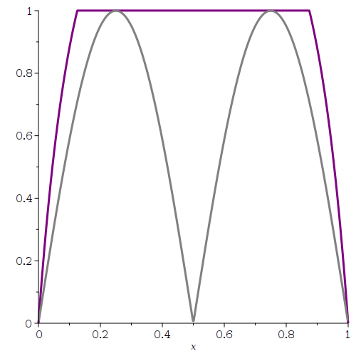
Heuristically, (3.13) seems to offer a good trade-off. For the above choice of we have , and applications of Section 3.1 are presented in Figure 1. Let us stress the similarity of the optimal landscape function in Figure 1 with that found, by different methods, in [41, Section 3.1].
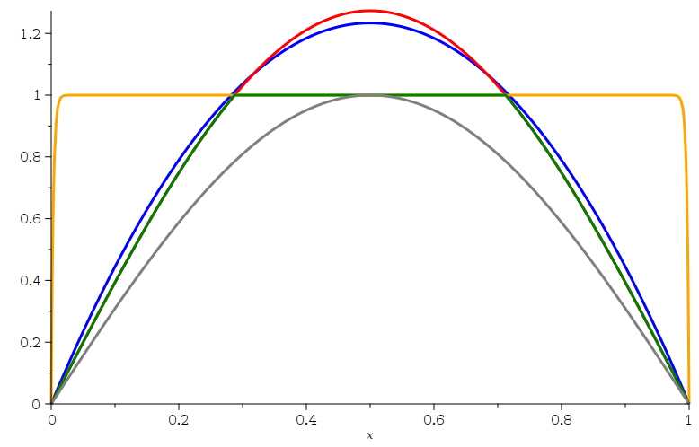
Right: An improved landscape function obtained by Section 3.1: we have plotted and in red and orange, respectively, and and their pointwise minimum – which by Section 3.1 dominates the ground state – in green. The canonical landscape function from [28] is plotted as well (in blue).
For comparison, we have also plotted the actual ground state, i.e., (in gray).
While it seems that, for the purpose of applying Section 3.1, there is no use in sampling at other positive values than for and , further improvement can be achieved by using the anti-maximum principle mentioned in Section 3.1.(1). Also, replacing by a smoother may allow for yet more precise estimates: taking , which is inspired by Section 3.1.(3), seems to be a smart choice, see Figure 2 (left).
Remark \therem.
Observe that is a polynomial of degree two. When applying Section 3.1, different polynomials can, of course, be considered as candidates for , as long as : this condition, however, is not always satisfied, as the choice of shows, as in this case fails to hold for any .
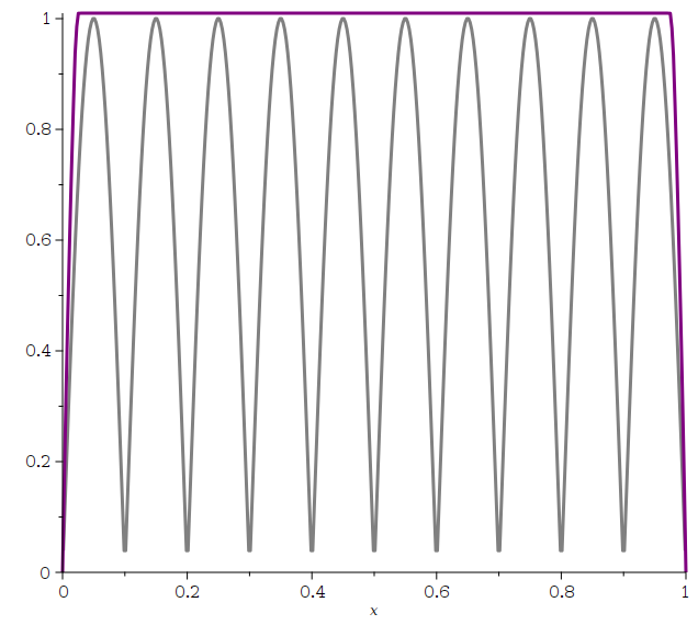
In the case of the present , it is even feasible to derive estimates based on the parabolic landscape function, as in Section 3.1. Indeed, expanding the -semigroup in Fourier series shows that (3.13) reads in this case
| (5.1) |
see Figure 2 (right): this bound has been found already in [41, Section 3.1].
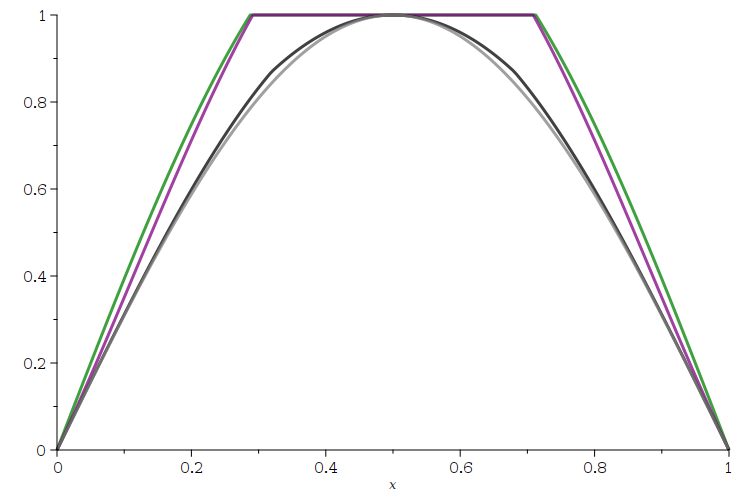
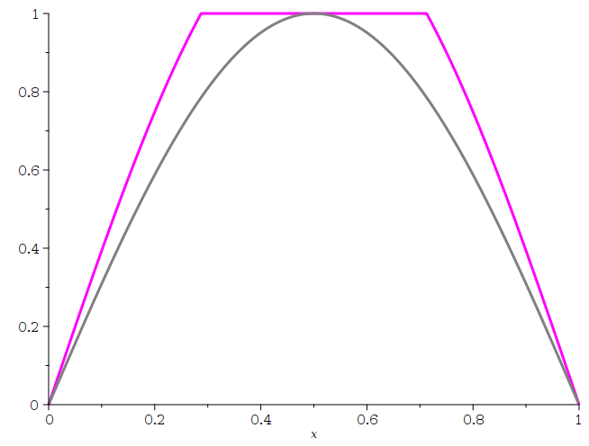
Right: A landscape function obtained applying the right estimate in (3.13): we have plotted in magenta the pointwise minimum of and . The function has been approximated truncating the series in (5.1) after the first 150 terms.
In gray: the actual ground state (both left and right).
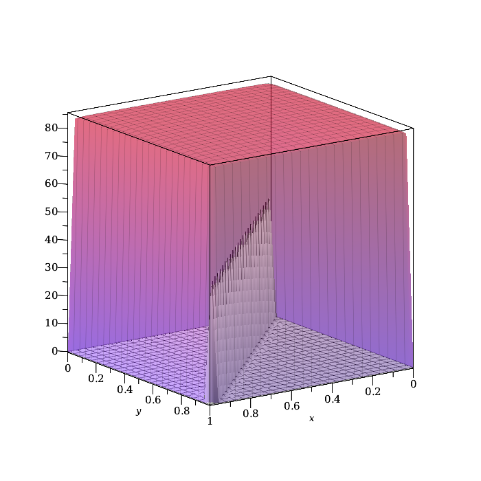
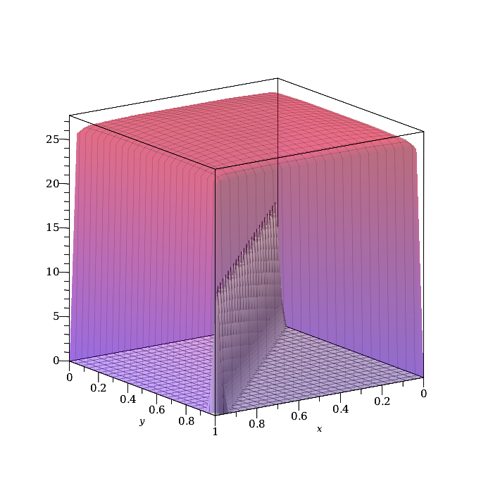
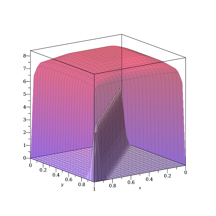
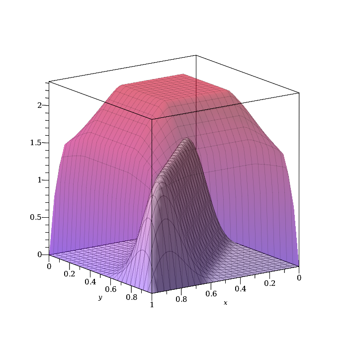
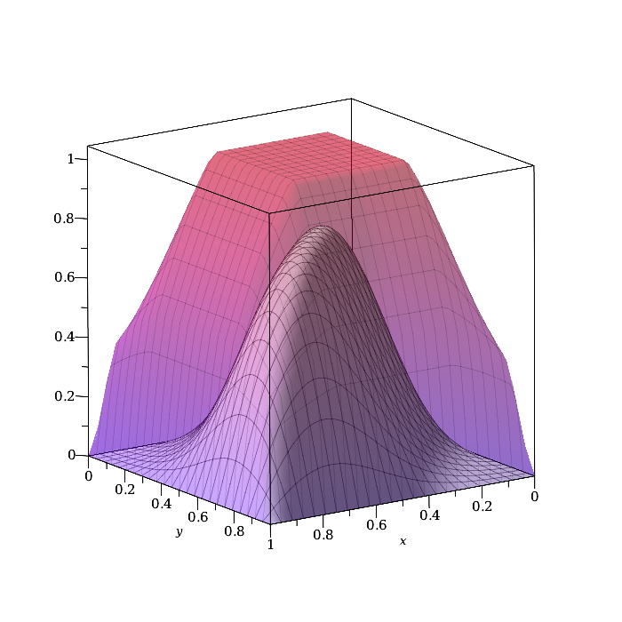
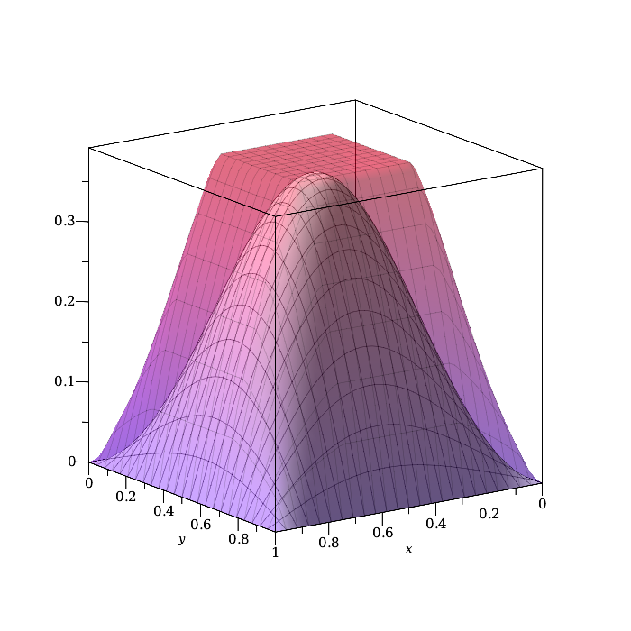
Figure 3 shows that our approach delivers reasonable pointwise eigenvector bounds even for higher eigenvalues. Indeed, by Section 3.1 we can use these estimates to deliver upper bounds on the heat kernel, see Figure 4. As the resolution of the eigenvector bound (3.11) becomes lower and lower for higher eigenvalues, the bound cannot capture the degeneracy of the heat kernel as , but is reasonably accurate for larger .
5.2. -Laplacians
Let us apply our theory to a common nonlinear operator: the -Laplacian on a bounded open set , for . We consider the energy functional defined by
or else by
for . Because is -homogeneous, its subdifferential is -homogeneous: indeed, is (minus) the -Laplacian with Dirichlet or Robin boundary conditions, i.e.,
| (5.3) |
respectively: let us take . Then is accretive; it is invertible whenever endowed with Dirichlet or (for ) Robin conditions.
Proposition \theprop.
Let be a bounded open domain. Then, for each , each eigenpair of the -Laplacian with either Dirichlet or Robin boundary conditions as in (5.3), for , satisfies
| (5.4) |
Furthermore, the lowest eigenvalue satisfies
| (5.5) |
and, in the case of Dirichlet boundary conditions, we find for the Cheeger constant
| (5.6) |
Proof.
We only have to show that is order preserving: that is, we assume and have to show that . The proof is similar to that of [10, Theorem 2.1]: integrate against and, using the Gauss–Green formulae and the boundary conditions, obtain
where the last inequality holds because is monotone: hence and therefore . The claim follows observing that all eigenvectors of with Dirichlet or Robin boundary conditions are essentially bounded, see [47, Theorem 4.1 and Corollary 4.2], and applying Section 2.
In the special case of Dirichlet conditions, (5.5) has already been obtained in [5, Theorem 1] in the case of and ; and in [33, Lemma 4.1] for general , but for domains with smooth boundary only. Also the lower estimate on in [33, Theorem 4.2] remains true under our milder assumptions on , as its proof is only based on Schwarz symmetrisation and the estimate (5.5).
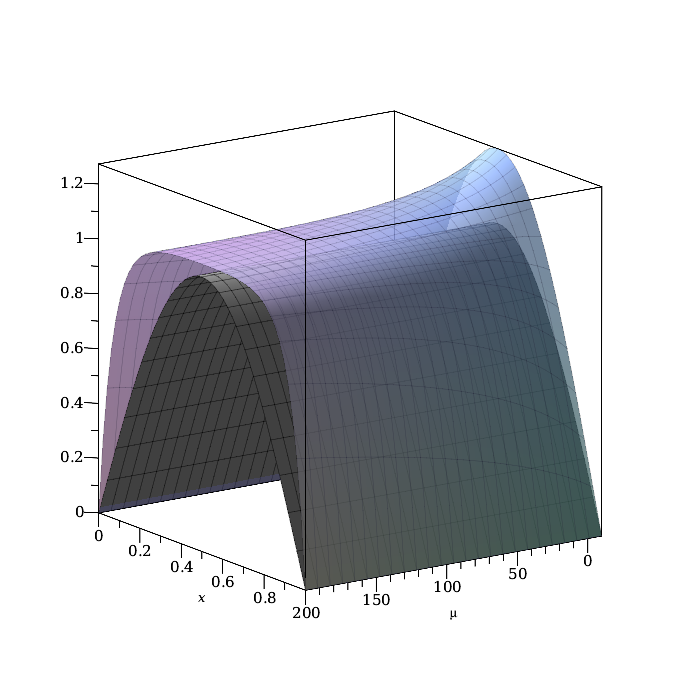
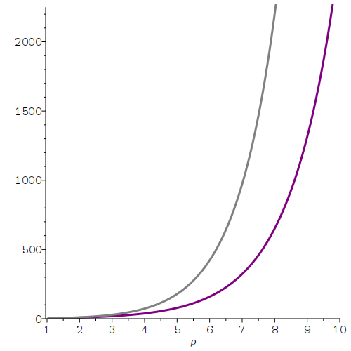
Let us now focus on the 1D case with Dirichlet boundary conditions: if , then
as shown by a direct computation. Its maximum is clearly attained at , and (5.5) reads
| (5.7) |
Indeed, it is well-known that , where : a comparison of the left and right hand sides of (5.7) is shown in Figure 5 (left). Also, it is easy to see that the Cheeger constant of is , while (5.6) yields
The estimate (5.4) is also remarkable because the -trigonometric function – which in turn yields the (-normalized) ground state
of the -Laplacian with Dirichlet conditions on – is only defined implicitly as the inverse of
see [46, Section 2.1]; even numerical plots of are not entirely trivial to obtain, cf. [31, 34]. The numerical values of obtained in Figure 5 (right) are in good agreement with the plots of the ground state of obtained in [31, Abbildung 2] by Matlab 5.3.
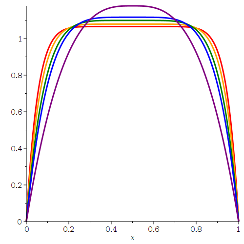
Right: A plot of for (in red), (in orange), (in green), (in blue), and (in purple).
Similar considerations hold, too, for the discrete -Laplacian with Dirichlet conditions on the boundary of any proper subgraph. Indeed, it is known that is invertible and its inverse is order preserving, see e.g. [61, Theorem A], so Section 2 can be applied. In the case of the -Laplacian (-Laplacian for ) on the unweighted path graph on 5 vertices with Dirichlet conditions at the extremal vertices , using symmetry arguments and running a numerical minimization on Mathematica Hua has found [42] that the (-normalized) ground state has the entries
with associated eigenvalue
By comparison, a numeric computation yields that the torsion function for the same graph is the vector
and we derive from Section 2 the estimate
5.3. Magnetic Schrödinger operators
Let us finally provide a local bound for the eigenvectors of Schrödinger operators with both electric and magnetic potential and , respectively: they are formally given by
Precisely introducing these operators is technical, but nowadays standard: based on quadratic form methods, on bounded open sets the realizations (resp., ) of with Dirichlet (resp., Neumann) conditions can be defined as self-adjoint operators on whenever , with and relatively form bounded with respect to the free Laplacian with Dirichlet (resp., Neumann) conditions, with relative bound . Details can be found in [43] and references therein.
In 1D, finding a landscape function for such operators is trivial, since the magnetic potential can be gauged away by the local unitary transformation . Accordingly, the eigenvectors of the magnetic Schrödinger operators have, at any point , same modulus as their non-magnetic counterparts and Section 3.1 yields no novel information in this case.
In higher dimension, though, the issue of bounding eigenvectors of magnetic Schrödinger operators is subtler: the torsion function of the non-magnetic Schrödinger operator has been proved in [41, Theorem 1] to be a landscape function for all Schrödinger operators with same electric potential but arbitrary magnetic potential, and a corresponding parabolic landscape function has been obtained in [41, Theorem 2]. The proof is based on stochastic arguments, and in particular on a Feynman–Kac-type formula: unsurprisingly, all results in [41] hold under smoothness assumptions on and the boundary of ; only Dirichlet conditions and are allowed. Let us remove these restrictions and state the following general result.
Proposition \theprop.
Let be a bounded open domain. Let the potentials be real-valued and such that , with , and let relatively form bounded, with relative bound , with respect to (resp., ). Then each eigenpair of (resp., of ) satisfies
| (5.8) |
| (5.9) |
Also,
| (5.10) |
| (5.11) |
The above estimates remain true if the landscape functions in the right hand sides are replaced by and , respectively (resp., and , respectively).
Furthermore, the bottom of the spectrum of satisfies
| (5.12) |
Proof.
To obtain the first four bounds, combine [43, Theorem 1.1 and Remark 1.2.(iii)] with Section 3.1.
The last estimate follows from Section 4. ∎
Likewise, we obtain a discrete version of Section 5.3: we follow the terminology and notation in Section 3.1.(3). In particular, given any graph and any magnetic signature we denote by the corresponding magnetic Laplacian; and, especially, by and the standard Laplacian and signless Laplacian, respectively. The realizations of (and ) with Dirichlet conditions at the boundary of some proper subgraphs will be denoted by (and, especially, ); it is well-known that they are invertible. All these operators are self-adjoint, and so are their versions with non-trivial, real-valued electric potential .
Proposition \theprop.
Let be a finite, weighted, undirected graph, and let some proper subgraph. Then for any real-valued potential each eigenpair of satisfies both
| (5.14) |
and
| (5.15) |
where denotes the largest eigenvalue of .
Proof.
The assertions are an immediate consequence of the Section 3.1, since
in view of the domination properties recalled in Section 3.1.(3) and of the fact that is an eigenpair of . ∎
Even restricting to , (5.14) sharpens the main estimate in [48], as is, by construction, dominated by the inverse of Ostrowski’s comparison matrix introduced in [48, Equation (3)]; while (5.15) should be compared with the high-energy eigenvectors bound by means of the dual landscape function obtained in [53, Corollary 4], which however only discusses non-magnetic Laplacians on path graphs.
References
- [1] F. Andreu-Vaillo, J.M. Mazón, J.D. Rossi, and J.J. Toledo-Melero. Nonlocal Diffusion Problems, volume 165 of Math. Surveys and Monographs. Amer. Math. Soc., Providence, RI, 2010.
- [2] W. Arendt and A.V. Bukhvalov. Integral representations of resolvents and semigroups. Forum Math., 6:111–135, 1994.
- [3] D.N. Arnold, G. David, M. Filoche, D. Jerison, and S. Mayboroda. Localization of eigenfunctions via an effective potential. Comm. Partial Differ. Equations, 44:1186–1216, 2019.
- [4] S. Arora and J. Glück. Criteria for eventual domination of operator semigroups and resolvents. arXiv:2204.00146, 2022.
- [5] R. Bañuelos and T. Carroll. Brownian motion and the fundamental frequency of a drum. Duke Math. J., 75:575–602, 1994.
- [6] S. Balasubramanian, Y. Liao, and V. Galitski. Many-body localization landscape. Phys. Rev. B, 101:014201, 2020.
- [7] Ph. Bénilan and M.G. Crandall. Completely accretive operators. In P. Clément, B. de Pagter, and E. Mitidieri, editors, Semigroup Theory and Evolution Equations, volume 135 of Lect. Notes Pure Appl. Math., pages 41–75. Dekker, Delft, 1991.
- [8] M. van den Berg. Estimates for the torsion function and Sobolev constants. Potential Analysis, 36:607–616, 2012.
- [9] P. Bifulco and J. Kerner. Comparing the spectrum of Schrödinger operators on quantum graphs. Proc. Amer. Math. Soc., 152:295–306, 2024.
- [10] V.E. Bobkov and P. Takáč. A strong maximum principle for parabolic equations with the -Laplacian. J. Math. Anal. Appl., 419:218–230, 2014.
- [11] T. Boggio. Sulle funzioni di Green d’ordine . Rend. Circ. Mat. Palermo, 20:97–135, 1905.
- [12] A. Bovier and F. Den Hollander. Metastability: a potential-theoretic approach, volume 351 of Grundlehren der mathematischen Wissenschaften. Springer, 2016.
- [13] A. Bovier, V. Gayrard, and M. Klein. Metastability in reversible diffusion processes II: Precise asymptotics for small eigenvalues. J. European Math. Soc., 7:69–99, 2005.
- [14] H. Brézis. Operateurs Maximaux Monotones et Semi-Groupes de Contractions dans les Espaces de Hilbert. North-Holland, Amsterdam, 1973.
- [15] L. Bungert and M. Burger. Asymptotic profiles of nonlinear homogeneous evolution equations of gradient flow type. J. Evol. Equ., 20:1061–1092, 2020.
- [16] R. Chill, D. Hauer, and J. Kennedy. Nonlinear semigroups generated by -elliptic functionals. J. Math. Pures Appl., 105:415–450, 2014.
- [17] F. Cipriani and G. Grillo. Nonlinear Markov semigroups, nonlinear Dirichlet forms and applications to minimal surfaces. J. Reine Ang. Math., 562:201–235, 2003.
- [18] Ph. Clément and L.A. Peletier. An anti-maximum principle for second-order elliptic operators. J. Differ. Equ., 34:218–229, 1979.
- [19] Y. Colin de Verdière, N. Torki-Hamza, and F. Truc. Essential self-adjointness for combinatorial Schrödinger operators. III: Magnetic fields. Ann. Fac. Sci. Toulouse, 20:599–611, 2011.
- [20] D. Daners, J. Glück, and J.B. Kennedy. Eventually and asymptotically positive semigroups on Banach lattices. J. Differ. Equ., 261:2607–2649, 2016.
- [21] E.B. Davies. Heat Kernels and Spectral Theory, volume 92 of Cambridge Tracts Math. Cambridge Univ. Press, Cambridge, 1989.
- [22] L.M. Del Pezzo and J.D. Rossi. The first eigenvalue of the -Laplacian on quantum graphs. Analysis and Math. Phys., 6:365–391, 2016.
- [23] F. del Teso, D. Gómez-Castro, and J.L. Vázquez. Three representations of the fractional -Laplacian: semigroup, extension and Balakrishnan formulas. Fract. Calc. Appl. Anal., 24:966–1002, 2021.
- [24] M.D. Donsker and S.R.S. Varadhan. On a variational formula for the principal eigenvalue for operators with maximum principle. Proc. Natl. Acad. Sci. USA, 72:780–783, 1975.
- [25] M.D. Donsker and S.R.S. Varadhan. On the principal eigenvalue of second-order elliptic differential operators. Comm. Pure Appl. Math., 29:595–621, 1976.
- [26] K.-J. Engel and R. Nagel. One-Parameter Semigroups for Linear Evolution Equations, volume 194 of Graduate Texts in Mathematics. Springer-Verlag, New York, 2000.
- [27] V. Ferone and B. Kawohl. Remarks on a finsler-laplacian. Proc. Amer. Math. Soc., 137:247–253, 2009.
- [28] M. Filoche and S. Mayboroda. Universal mechanism for Anderson and weak localization. Proc. Natl. Acad. Sci. USA, 109:14761–14766, 2012.
- [29] M. Filoche and S. Mayboroda. Universal mechanism for Anderson and weak localization – supporting information: Mathematical proofs. http://www.pnas.org/lookup/suppl/doi:10.1073/pnas.1120432109/-/DCSupplemental/Appendix.pdf, 2012.
- [30] M. Filoche, S. Mayboroda, and T. Tao. The effective potential of an -matrix. J. Math. Phys., 62:041902, 2021.
- [31] V. Fridman. Das Eigenwertproblem zum -Laplace Operator für gegen 1. PhD thesis, Universität zu Köln, 2003.
- [32] S. Fučík, J. Nečas, J. Souček, and V. Souček. Spectral Analysis of Nonlinear Operators, volume 346 of Lect. Notes Math. Springer-Verlag, Berlin, 1973.
- [33] T. Giorgi and R.G. Smits. Principal eigenvalue estimates via the supremum of torsion. Indiana Univ. Math. J., 59:987–1011, 2010.
- [34] P. Girg and L. Kotrla. Differentiability properties of -trigonometric functions. Electronic J. Differ. Equ., 21:101–127, 2014.
- [35] J. Glück. Evolution equations with eventually positive solutions. EMS Magazine, pages 4–11, 2022.
- [36] J. Glück and D. Mugnolo. Eventual domination for linear evolution equations. Math. Z., 299:1421–1433, 2021.
- [37] W. Górny and J.M. Mazón. On the -Laplacian evolution equation in metric measure spaces. arXiv:2103.13373.
- [38] E.M. Harrell and A.V. Maltsev. Localization and landscape functions on quantum graphs. Trans. Amer. Math. Soc., 373:1701–1729, 2020.
- [39] B. Helffer. Semi-classical analysis for the Schrödinger operator and applications, volume 1336 of Lect. Notes Math. Springer-Verlag, Berlin, 1988.
- [40] P.D. Hislop and I.M. Sigal. Introduction to spectral theory: with applications to Schrödinger operators, volume 113 of Appl. Math. Sci. Springer-Verlag, New York, 1996.
- [41] J.G. Hoskins, H. Quan, and S. Steinerberger. Magnetic Schrödinger operators and landscape functions. arXiv:2210.02646.
- [42] B. Hua. Private communication, 2022.
- [43] D. Hundertmark and B. Simon. A diamagnetic inequality for semigroup differences. J. Reine Angew. Math., 571:107–130, 2004.
- [44] B. Kawohl. How I met the normalized -Laplacian and what we know now about mean values and concavity properties. Journal of Elliptic and Parabolic Equations, 6:113–121, 2020.
- [45] B. Kawohl and V. Fridman. Isoperimetric estimates for the first eigenvalue of the -Laplace operator and the Cheeger constant. Comment. Math. Univ. Carolin., 44:659–667, 2003.
- [46] J. Lang and D. Edmunds. Eigenvalues, Embeddings, and Generalised Trigonometric Functions, volume 2016 of Lect. Notes Math. Springer-Verlag, Berlin, 2011.
- [47] A. Lê. Eigenvalue problems for the -Laplacian. Nonlinear Anal., Theory Methods Appl., 64:1057–1099, 2006.
- [48] G. Lemut, M.J. Pacholski, O. Ovdat, A. Grabsch, J. Tworzydło, and C.W.J. Beenakker. Localization landscape for Dirac fermions. Phys. Rev. B, 101:081405, 2020.
- [49] D. Lenz, M. Schmidt, and M. Wirth. Uniqueness of form extensions and domination of semigroups. J. Funct. Anal., 280:108848, 2021.
- [50] E.H. Lieb and R. Seiringer. The Stability of Matter in Quantum Mechanics. Cambridge Univ. Press, Cambridge, 2010.
- [51] J. Lu and S. Steinerberger. A variation on the Donsker–Varadhan inequality for the principal eigenvalue. Proc. Royal Soc. London A, 473(2204):20160877, 2017.
- [52] J. Lu and S. Steinerberger. Detecting localized eigenstates of linear operators. Research Math. Sci., 5:1–14, 2018.
- [53] M.L. Lyra, S. Mayboroda, and M. Filoche. Dual landscapes in Anderson localization on discrete lattices. Europhys. Letters, 109:47001, 2015.
- [54] M. Melgaard, E.M. Ouhabaz, and G. Rozenblum. Negative discrete spectrum of perturbed multivortex Aharonov–Bohm Hamiltonians. Ann. Henri Poincaré A, 5:979–1012, 2004.
- [55] D. Mugnolo. Parabolic theory of the discrete -Laplace operator. Nonlinear Anal., Theory Methods Appl., 87:33–60, 2013.
- [56] D. Mugnolo. Semigroup Methods for Evolution Equations on Networks. Underst. Compl. Syst. Springer-Verlag, Berlin, 2014.
- [57] D. Mugnolo and M. Plümer. On torsional rigidity and ground-state energy of compact quantum graphs. Calc. Var., 62:27, 2023.
- [58] R. Nagel, editor. One-Parameter Semigroups of Positive Operators, volume 1184 of Lect. Notes Math. Springer-Verlag, Berlin, 1986.
- [59] M. Ôtani. A remark on certain nonlinear elliptic equations. Proc. Fac. Sci. Tokai Univ., 19:23–28, 1984.
- [60] E.M. Ouhabaz. Analysis of Heat Equations on Domains, volume 30 of Lond. Math. Soc. Monograph Series. Princeton Univ. Press, Princeton, NJ, 2005.
- [61] J.-H. Park. On a resonance problem with the discrete -Laplacian on finite graphs. Nonlinear Anal., Theory Methods Appl., 74:6662–6675, 2011.
- [62] G. Pólya. Torsional rigidity, principal frequency, electrostatic capacity and symmetrization. Quart. Appl. Math, 6:267–277, 1948.
- [63] H.H. Schaefer. Banach Lattices and Positive Operators, volume 215 of Grundlehren der mathematischen Wissenschaften. Springer-Verlag, Berlin, 1974.
- [64] S. Steinerberger. Localization of quantum states and landscape functions. Proc. Amer. Math. Soc., 145:2895–2907, 2017.
- [65] S. Steinerberger. Regularized potentials of Schrödinger operators and a local landscape function. Comm. Partial Differ. Equations, 46:1262–1279, 2021.
- [66] W. Wang and S. Zhang. The exponential decay of eigenfunctions for tight-binding Hamiltonians via landscape and dual landscape functions. Ann. Henri Poincaré, 22:1429–1457, 2021.