Almost Surely $\sqrt{T}$ Regret Bound for Adaptive LQR

Abstract

The Linear-Quadratic Regulation (LQR) problem with unknown system parameters has been widely studied, but it has remained unclear whether $\tilde{\mathcal{O}}(\sqrt{T})$ regret, which is the best known dependence on time, can be achieved almost surely. In this paper, we propose an adaptive LQR controller with almost surely $\tilde{\mathcal{O}}(\sqrt{T})$ regret upper bound. The controller features a circuit-breaking mechanism, which circumvents potential safety breach and guarantees the convergence of the system parameter estimate, but is shown to be triggered only finitely often and hence has negligible effect on the asymptotic performance of the controller. The proposed controller is also validated via simulation on Tennessee Eastman Process (TEP), a commonly used industrial process example.

I Introduction

Adaptive control, the study of decision-making under the parametric uncertainty of dynamical systems, has been pursued for decades [1, 2, 3, 4]. Although early research mainly focused on the the aspect of convergence and stability, recent years have witnessed significant advances in the quantitative performance analysis of adaptive controllers, especially for multivariate systems. In particular, in the adaptive Linear-Quadratic Regulation (LQR) setting considered in this paper, the controller attempts to solve the stochastic LQR problem without access to the true system parameters, and its performance is evaluated via regret, the cumulative deviation from the optimal cost over time. This adaptive LQR setting has been widely studied in the past decade [5, 6, 7, 8, 9, 10, 11], but it has remained unclear whether adaptive controllers for LQR can achieve $\tilde{\mathcal{O}}(\sqrt{T})$ regret, whose asymptotic dependence on the time $T$ is the best known (up to poly-logarithmic factors) , almost surely.

Existing regret upper bounds on adaptive LQR, summarized in Table I, are either weaker than almost-sure in terms of the type of probabilistic guarantee, or suboptimal in terms of asymptotic dependence on time. By means of optimism-in-face-of-uncertainty [7], Thompson sampling [6], or $\epsilon$-greedy algorithm [9], an $\tilde{\mathcal{O}}(\sqrt{T})$ regret can be achieved with probability at least $1-\delta$. In other words, these algorithms may not converge to the optimal one or could even be destablizing with a non-zero probability $\delta$. In practice, such a failure probability may hinder the application of these algorithms in safety-critical scenarios. From a theoretical perspective, we argue that it is highly difficult to extend these algorithms to provide stronger performance guarantees. To be specific, despite different exploration strategies, the aforementioned methods all compute the control input using a linear feedback gain synthesized from a least-squares estimate of system parameters. Due to Gaussian process noise, the derived linear feedback gain may be destabilizing, regardless of the amount of data collected. For these algorithms, the probability of such catastrophic event is bounded by a positive $\delta>0$, which is a predetermined design parameter and cannot be changed during online operation.

Alternative methods that may preclude the above described failure probability include introducing additional stability assumptions, using parameter estimation algorithms with stronger convergence guarantees, and adding a layer of safeguard around the linear feedback gain. Faradonbeh et al. [10] achieves $\tilde{\mathcal{O}}(\sqrt{T})$ regret almost surely under the assumption that the closed-loop system remains stable all the time, based on a stabilization set obtained from adaptive stabilization [12]. Since the stabilization set is estimated from finite data and violates the desired property with a nonzero probability, this method essentially has a nonzero failure probability as well. Guo [13] achieves sub-linear regret almost surely by adopting a variant of ordinary least squares with annealing weight assigned to recent data, a parameter estimation algorithm convergent even with unstable trajectory data. However, the stronger convergence guarantee may come at the cost of less sharp asymptotic rate, and it is unclear whether the regret of this method can achieve $\tilde{\mathcal{O}}(\sqrt{T})$ dependence on time. Wang and Janson [11] achieves $\tilde{\mathcal{O}}(\sqrt{T})$ regret with a convergence-in-probability guarantee, via the use of a switched, rather than linear feedback controller, which falls back to a known stabilizing gain on the detection of large states. However, the controller design of this work does not rule out the frequent switching between the learned and fallback gains, a typical source of instability in switched linear systems [14], which restricts the correctness of their results to the case of commutative closed-loop system matrices. Moreover, the regret analysis in this work is not sufficiently refined to lead to almost sure guarantees.

TABLE I: Comparison with selected existing works on adaptive LQR

Work	Rate	Type of guarantee
[13]	Not provided	Almost sure
[7, 6, 9]	$\tilde{\mathcal{O}}(\sqrt{T})$	Probability $1-\delta$
[10]	$\tilde{\mathcal{O}}(\sqrt{T})$	Almost sure*
[11]	$\tilde{\mathcal{O}}(\sqrt{T})$	Convergence in probability*
This work	$\tilde{\mathcal{O}}(\sqrt{T})$	Almost sure

• Requires non-standard assumptions; please refer to the main text for details.

In this paper, we present an adaptive LQR controller with $\tilde{\mathcal{O}}(\sqrt{T})$ regret almost surely, only assuming the availability of a known stabilizing feedback gain, which is a common assumption in the literature. This is achieved by a “circuit-breaking” mechanism motivated similarly as [11], which circumvents safety breach by supervising the norm of the state and deploying the feedback gain when necessary. In contrast to [11], however, by enforcing a properly chosen dwell time on the fallback mode, the stability of the closed-loop system under our proposed controller is unaffected by switching. Another insight underlying our analysis is that the above mentioned circuit-breaking mechanism is triggered only finitely often. This fact implies that the conservativeness of the proposed controller, which prevents the system from being destabilized in the early stage and hence ensures the convergence of the system parameter estimates, may have negligible effect on the asymptotic performance of the system. Although similar phenomena have also been observed in [15, 11], we derive an upper bound on the time of the last trigger (Theorem 3, item 27)), a property missing from pervious works that paves the way to our almost sure regret guarantee.

Outline

The remainder of this manuscript is organized as follows: Section II introduces the problem setting. Section III describes the proposed controller. Section IV states and proves the theoretical properties of the closed-loop system under the proposed controller, and establishes the main regret upper bound. Section V validates the theoretical results using a numerical example. Finally, Section VI summarizes the manuscript and discusses directions for future work.

Notations

The set of nonnegative integers is denoted by $\mathbb{N}$, and the set of positive integers is denoted by $\mathbb{N}^{*}$. The $n$-dimensional Euclidean space is denoted by $\mathbb{R}^{n}$, and the $n$-dimensional unit sphere is denoted by $\mathbb{S}^{n}$. The $n\times n$ identity matrix is denoted by $I_{n}$. For a square matrix $M$, $\rho(M)$ denotes the spectral radius of $M$, and $\operatorname{tr}(M)$ denotes the trace of $M$. For a real symmetric matrix $M$, $M\succ 0$ denotes that $M$ is positive definite. For any matrix $M$, $M^{\dagger}$ denotes the Moore-Penrose inverse of $M$. For two vectors $u,v\in\mathbb{R}^{n}$, $\langle u,v\rangle$ denotes their inner product. For a vector $v$, $\|v\|$ denotes its 2-norm, and $\|v\|_{P}=\|P^{1/2}v\|$ for $P\succ 0$. For a matrix $M$, $\|M\|$ denotes its induced 2-norm, and $\|M\|_{F}$ denotes its Frobenius norm. For a random vector $x$, $x\sim\mathcal{N}(\mu,\Sigma)$ denotes $x$ is Gaussian distributed with mean $\mu$ and covariance $\Sigma$. For a random variable $X$, $X\sim\chi^{2}(n)$ denotes $X$ has a chi-squared distribution with $n$ degrees of freedom. $\mathbb{P}(\cdot)$ denotes the probability operator, and $\mathbb{E}[\cdot]$ denotes the expectation operator.

For non-negative quantities $f,g$, which can be deterministic or random, we say $f\lesssim g$ to denote that $f\leq C_{1}g+C_{2}$ for some universal constants $C_{1}>0$ and $C_{2}>0$, and $f\gtrsim g$ to denote that $g\lesssim f$. For a random function $f(T)$ and a deterministic function $g(T)$, we say $f(T)=\mathcal{O}(g(T))$ to denote that $\limsup_{T\to\infty}f(T)/g(T)<\infty$, and $f(T)=\tilde{\mathcal{O}}(g(T))$ to denote that $f(T)=\mathcal{O}(g(T)(\log(T))^{\alpha})$ for some $\alpha>0$.

II Problem formulation

This paper considers a fully observed discrete-time linear system with Gaussian process noise specified as follows:

$$x_{k+1}=Ax_{k}+Bu_{k}+w_{k},\quad k\in\mathbb{N}^{*},\quad x_{1}=0,$$ (1)

where $x_{k}\in\mathbb{R}^{n}$ is the state, $u_{k}\in\mathbb{R}^{m}$ is the control input, and $w_{k}\stackrel{{\scriptstyle\text{ i.i.d. }}}{{\sim}}\mathcal{N}(0,W)$ is the process noise, where $W\succ 0$. It is assumed without loss of generality that $W=I_{n}$, but all the conclusions apply to general positive definite $W$ up to the scaling of constants. It is also assumed that the system and input matrices $A,B$ are unknown to the controller, but $(A,B)$ is controllable, and that the system is open-loop stable, i.e., $\rho(A)<1$. Consequently, there exists $P_{0}\succ 0$ that satisfies the discrete Lyapunov equation

$$A^{\top}P_{0}A-P_{0}+Q=0,$$ (2)

and there exists a scalar $0<\rho_{0}<1$ such that

$$A^{\top}P_{0}A\prec\rho_{0}P_{0}.$$ (3)

Remark 1.

It has been commonly assumed in the literature [9, 11] that $(A,B)$ being stabilizable by a known feedback gain $K_{0}$, i.e., $\rho(A+BK_{0})<1$. In such case, the system can be rewritten as

$$x_{k+1}=A^{\prime}x_{k}+Bu_{k}^{\prime}+w_{k},$$ (4)

where $A^{\prime}=A+BK_{0},u_{k}^{\prime}=u_{k}-K_{0}x_{k}$, which reduces the problem to the case of open-loop stable systems. Therefore, we may assume without loss of generality that the system is open-loop stable, i.e., $K_{0}=0$, for the simplicity of notations.

The following average infinite-horizon quadratic cost is considered:

$$J=\limsup_{T\rightarrow\infty}\frac{1}{T}\mathbb{E}\left[\sum_{k=1}^{T}x_{k}^{\top}Qx_{k}+u_{k}^{\top}Ru_{k}\right],$$ (5)

where $Q\succ 0,R\succ 0$ are fixed weight matrices specified by the system operator. It is well known that the optimal control law is the linear feedback control law of the form $u(x)=K^{*}x$, where the optimal feedback gain $K^{*}$ can be specified as:

$$K^{*}=-\left(R+B^{\top}P^{*}B\right)^{-1}B^{\top}P^{*}A,$$ (6)

and $P^{*}$ is the unique positive definite solution to the discrete algebraic Riccati equation

$$P^{*}=A^{\top}P^{*}A-A^{\top}P^{*}B\left(R+B^{\top}P^{*}B\right)^{-1}B^{\top}P^{*}A+Q.$$ (7)

The corresponding optimal cost is

$$J^{*}=\operatorname{tr}\left(\mathbb{E}\left[w_{k}w_{k}^{\top}\right]P^{*}\right)=\operatorname{tr}(WP^{*})=\operatorname{tr}(P^{*}).$$ (8)

The matrix $P^{*}$ also satisfies the discrete Lyapunov equation

$$(A+BK^{*})^{\top}P^{*}(A+BK^{*})-P^{*}+Q+K^{\top}RK=0,$$ (9)

which implies that there exists a scalar $0<\rho^{*}<1$ such that

$$(A+BK^{*})^{\top}P^{*}(A+BK^{*})\prec\rho^{*}P^{*}.$$ (10)

Since $A,B$ are unknown to the controller in the considered setting, it is not possible to directly compute the optimal control law from (6) and (7). Instead, the controller learns the optimal control law online, whose performance is measured via the regret defined as follows:

$$\mathcal{R}(T)=\sum_{k=1}^{T}(x_{k}^{\top}Qx_{k}+u_{k}^{\top}Ru_{k})-TJ^{*}.$$ (11)

The goal of the controller is to minimize the asymptotic growth of $\mathcal{R}(T)$.

III Controller design

The logic of the proposed controller is presented in Algorithm 1. It can also be illustrated by the block diagram in Fig. 1. The remainder of this section would be devoted to explaining the components of the controller:

1:$\hat{K}_{0}\leftarrow 0$

2:$\xi\leftarrow 0$

3:for $k=1,2,\ldots$ do

4:     Update parameter estimates $\hat{A}_{k},\hat{B}_{k}$ using (12)

5:     if $(\hat{A}_{k},\hat{B}_{k})$ is controllable then

6:         Update $\hat{K}_{k}$ from (6)-(7), replacing $(A,B)$ with $(\hat{A}_{k},\hat{B}_{k})$.

7:     else

8:         $\hat{K}_{k}\leftarrow 0$      

9:     $u^{ce}_{k}\leftarrow\hat{K}_{k}x_{k}$

10:     if $\xi=0$ then

11:         if  $\max\{\|u^{ce}_{k}\|,\|\hat{K}_{k}\|\}>M_{k}:=\log(k)$  then

12:              $\xi\leftarrow t_{k}:=\lfloor\log(k)\rfloor$

13:              $u^{cb}_{k}\leftarrow 0$

14:         else

15:              $u^{cb}_{k}\leftarrow u^{ce}_{k}$          

16:     else

17:         $u^{cb}_{k}\leftarrow 0$

18:         $\xi\leftarrow\xi-1$      

19:     $u^{pr}_{k}\leftarrow k^{-1/4}v_{k}$, where $v_{k}\sim\mathcal{N}(0,I_{m})$

20:     Apply $u_{k}\leftarrow u^{cb}_{k}+u^{pr}_{k}$

Algorithm 1 Proposed controller

Figure 1: Block diagram of the closed-loop system under the proposed controller. The control input is the superposition of a deterministic input $u^{cb}$ and a random probing input $u^{pr}$. The deterministic part $u^{cb}$ is normally the same as the certainty equivalent input $u^{ce}$, but takes the value zero when circuit-breaking is triggered, where $\xi$ is a counter for circuit-breaking. The certainty equivalent gain is updated using the parameter estimator in the meantime.

The proposed controller is a variant of the certainty equivalent controller [16], where the latter applies the input $u^{ce}_{k}=\hat{K}_{k}x_{k}$, where the feedback gain $\hat{K}_{k}$ is calculated from (6)-(7) by treating the current estimates of the system parameters $\hat{A}_{k},\hat{B}_{k}$ as the true values. The differences of the proposed controller compared to the standard certainty equivalent controller is that i) it includes a “circuit-breaking” mechanism, which replace $u^{ce}_{k}$ with zero in certain circumstances; ii) it superposes the control input at each step with a probing noise $u^{pr}_{k}$.

The circuit-breaking mechanism replaces $u^{ce}_{k}$ with zero for the subsequent $t_{k}$ steps when either the norm of the certainty equivalent control input $\|u^{ce}_{k}\|$ of the norm of the certainty equivalent feedback gain $\|\hat{K}_{k}\|$ exceeds a threshold $M_{k}$. The intuition behind this design is that a large certainty equivalent control input is indicative of having applied a destabilizing feedback gain recently, and circuit-breaking may prevent the state from exploding by leveraging the innate stability of the system, and hence help with the convergence of the parameter estimator and the asymptotic performance of the controller. The threshold $M_{k}$ is increased with the time index $k$, so that the “false alarm rate” of circuit-breaking, caused by the occasional occurrence of large noise vectors, decays to zero. The dwell time $t_{k}$ is also increased with time, in order to circumvent the potential oscillation of the system caused by the frequent switching between $\hat{K}$ and $0$ (c.f. [17]). Both $M_{k}$ and $t_{k}$ are chosen to grow logarithmically with $k$, which would support our technical guarantees.

Similarly to [9, 11], a probing noise $u_{k}^{pr}$ is superposed to the control input at each step to provide sufficient excitation to the system, which is required for the estimation of system parameters. Specifically, the probing noise is chosen to be $u_{k}^{pr}=k^{-1/4}v_{k}$, where $v_{k}\stackrel{{\scriptstyle\text{ i.i.d. }}}{{\sim}}\mathcal{N}(0,I_{m})$, which would correspond to the optimal rate of regret.

The estimates of the system parameters $\hat{A}_{k},\hat{B}_{k}$ are updated using an ordinary least squares estimator. Denote $\Theta=[A\quad B]$, $\hat{\Theta}_{k}=[\hat{A}_{k}\quad\hat{B}_{k}]$, and $z_{k}=[x_{k}^{\top}\quad u_{k}^{\top}]^{\top}$, then according to $x_{k+1}=\Theta z_{k}$, the ordinary least squares estimator can be specified as

$$\hat{\Theta}_{k}=\left(\sum_{t=1}^{k-2}x_{t+1}z_{t}^{\top}\right)\left(\sum_{t=1}^{k-2}z_{t}z_{t}^{\top}\right)^{\dagger}.$$ (12)

Remark 2.

In the presented algorithm, the certainty equivalent gain is updated at every step $k$ (see line 6 of Algorithm 1), but it may also be updated “logarithmically often” [11] (e.g., at steps $k=2^{i},i\in\mathbb{N}^{*}$), which is more computationally efficient in practice. It can be verified that all our theoretical results also apply to the case of logarithmically often updates.

IV Main results

Underlying our analysis of the closed-loop system under the proposed controller are two random times, defined below:

$$T_{\text{stab}}:=\inf\left\{T\vphantom{\left(A^{\lfloor\log k\rfloor}\right)^{\top}}\right.\left|\left(A^{t_{k}}\right)^{\top}P^{*}A^{t_{k}}<\rho P^{*},\right.$$

$$\mkern 10.0mu\left.\vphantom{\left(A^{t_{k}}\right)^{\top}}\left(A+B\hat{K}_{k}\right)^{\top}P^{*}\left(A+B\hat{K}_{k}\right)<\rho P^{*},\forall k\geq T\right\},$$ (13)

where $\rho=(1+\rho^{*})/2$, and $t_{k}$ is the dwell time defined in line 12 of Algorithm 1. And

$$T_{\text{nocb}}:=\inf\left\{T\mid u_{k}^{cb}\equiv u_{k}^{ce},\forall k\geq T\right\}.$$ (14)

With the above two random times, the evolution of the system can be divided into three stages:

1. From the beginning to $T_{\text{stab}}$, the adaptive controller gradually refines its estimate of system parameters, and hence improves the performance of the certainty equivalent feedback gain, until the system becomes stabilized in the sense that there is a common Lyapunov function between the two modes under circuit-breaking as indicated in (13).

2. From $T_{\text{stab}}$ to $T_{\text{nocb}}$, the closed-loop system is stable as is ensured by the aforementioned common Lyapunov function, and under mild regularity conditions on the noise, an upper bound on the magnitude certainty equivalent control input $\|u^{ce}_{k}\|$ eventually drops below the circuit-breaking threshold $M_{k}$.

3. From $T_{\text{nocb}}$ on, circuit-breaking is not triggered any more, and the system behaves similarly as the closed-loop system under the optimal controller, with only small perturbations on the feedback gain which stem from the parameter estimation error and converge to zero.

In the following theorem, we state several properties of the closed-loop system, based on which the above two random times are quantified:

Theorem 3.

Let $n,m$ be the dimensions of the state and input vectors respectively, and $P_{0},\rho_{0},P^{*},\rho^{*}$ be defined in (2), (3), (7), (10) respectively. Then the following properties hold:

1. For $0<\delta\leq 1/2$, the event

   $$\mathcal{E}_{\text{noise}}(\delta):=\left\{\max\{\|w_{k}\|,\|v_{k}\|\}\leq\vphantom{\sqrt{()}}\right.$$

   $$\mkern 100.0mu\left.2\sqrt{n+1}\sqrt{\log(k/\delta)},\forall k\in\mathbb{N}^{*}\right\}$$ (15)

   occurs with probability at least $1-2\delta$.

2. For $0<\delta\leq 1/(8n^{2})$, the event

   $$\mathcal{E}_{\text{cov}}(\delta):=\left\{\left\|\sum_{i=1}^{k}(w_{i}w_{i}^{\top}-I_{n})\right\|\leq\right.$$

   $$\mkern 100.0mu\left.7n\sqrt{k}\log(8n^{2}k/\delta),\forall k\in\mathbb{N}^{*}\vphantom{\sum_{i}^{i}}\right\}$$ (16)

   occurs with probability at least $1-\delta$.

3. On the event $\mathcal{E}_{\text{noise}}(\delta)$, it holds

   $$\|x_{k}\|\leq C_{x}\log(k/\delta),\forall k\in\mathbb{N}^{*},$$ (17)

   where

   $$C_{x}=\frac{(\|B\|+1)(2\sqrt{n+1}+1)\|P_{0}\|\|P_{0}^{-1}\|}{1-\rho_{0}^{1/2}}.$$ (18)

4. For $0<\delta\leq 1/14$, the event

   $$\mathcal{E}_{\text{cross}}(\delta):=\left\{\vphantom{\sum_{i}^{i}}\right.$$

   $$\max\left\{\left\|\sum_{i=1}^{k}(w_{i}+Bu_{i}^{pr})^{\top}P^{*}(Ax_{i}+Bu^{cb}_{i})\right\|,\right.$$

   $$\mkern 50.0mu\left.\left\|\sum_{i=1}^{k}(u_{i}^{pr})^{\top}Ru_{i}^{cb}\right\|,\right.$$

   $$\mkern 50.0mu\left.\left\|\sum_{i=1}^{k}w_{i}^{\top}P^{*}Bu_{i}^{pr}\right\|\right\}\leq$$

   $$\mkern 100.0mu\left.C_{\text{cross}}\sqrt{k}(\log(k/\delta))^{2},\forall k\in\mathbb{N}^{*}\vphantom{\sum_{i}^{i}}\right\}$$ (19)

   occurs with probability at least $1-14\delta$, where

   $$C_{\text{cross}}=4\sqrt{n+1}(\|B\|+1)\cdot$$

   $$\quad(\|P^{*}\|\|A\|C_{x}+\|P^{*}\|\|B\|+\|R\|).$$ (20)

5. For $\delta$ satisfying

   $$0<\delta<\min\left\{(38400C_{V})^{-1},\exp\left(-22(m+n)^{1/3}\right)\right\},$$ (21)

   the event

   $$\mathcal{E}_{\text{est}}(\delta):=\left\{\left\|\hat{\Theta}_{k}-\Theta\right\|^{2}\leq C_{\Theta}k^{-1/2}(\log(k/\delta))^{3},\right.$$

   $$\mkern 100.0mu\left.\vphantom{\left\|\hat{\Theta}_{k}-\Theta\right\|^{2}}\forall k\geq k_{0}\right\},$$ (22)

   occurs with probability at least $1-6\delta$, where

   $$k_{0}=\lceil 4000(m+n)\log(1/\delta)\rceil,$$ (23)

   $$C_{V}=C_{x}+2\sqrt{n+1}+1,$$ (24)

   $$C_{\Theta}=(25600n/3)(5n/2+2).$$ (25)

6. On the event $\mathcal{E}_{\text{est}}(\delta)$, it holds

   $$T_{\text{stab}}\lesssim(\log(1/\delta))^{2}.$$ (26)

7. On the event $\mathcal{E}_{\text{noise}}(\delta)\cap\mathcal{E}_{\text{est}}(\delta)$, for any $\alpha>0$, it holds

   $$T_{\text{nocb}}\lesssim(1/\delta)^{\alpha}.$$ (27)

Remark 4.

The conclusions of Theorem 3 can be explained as follows:

Items 1) and 2) defines two high-probability events on the regularity of noise. Item 18) bounds the state norm under regular noise, based on which item 4) bounds the growth of a few cross terms that would be useful in regret analysis. Item 5) bounds the parameter estimation error, based on which item 26) bounds $T_{\text{stab}}$. Finally, item 27) states that the circuit-breaking mechanism is triggered only finitely, and bounds $T_{\text{nocb}}$, the time after which the circuit-breaking is not triggered any more.

The following corollary characterizes the tail probabilities of $T_{\text{stab}}$ and $T_{\text{nocb}}$, which follows directly from items 26) and 27) of Theorem 3:

Corollary 5.

For $T_{\text{stab}}$ defined in (13) and $T_{\text{nocb}}$ defined in (14), as $T\to\infty$, it holds

1. $$\mathbb{P}(T_{\text{stab}}\geq T)=\mathcal{O}(\exp(-c\sqrt{T})),$$ (28)

   where $c>0$ is a system-dependent constant.

2. For any $\alpha>0$,

   $$\mathbb{P}(T_{\text{nocb}}\geq T)=\mathcal{O}(T^{-\alpha}).$$ (29)

Building upon the properties stated in Theorem 3, a high-probability bound on the regret under the proposed controller can be ensured:

Theorem 6.

Given a failure probability $\delta$, there exists a constant $T_{0}\lesssim(1/\delta)^{1/4}$, such that for any fixed $T>T_{0}$, it holds with probability at least $1-\delta$ that the regret defined in (11) satisfies

$$\mathcal{R}(T)\lesssim(1/\delta)^{1/4}+\sqrt{T}(\log(T/\delta))^{5}.$$ (30)

As corollaries of Theorem 30, one can obtain a bound on the tail probability of $\mathcal{R}(T)$ (Theorem 7), and the main conclusion of this work, i.e., an almost sure bound on $\mathcal{R}(T)$ (Theorem 32):

Theorem 7.

For sufficiently large $T$, it holds

$$\mathbb{P}\left(\mathcal{R}(T)\geq C_{R}\sqrt{T}(\log(T))^{5}\right)\leq\frac{1}{T^{2}},$$ (31)

where $C_{R}$ is a system-dependent constant.

Proof.

The conclusion follows from invoking Theorem 30 with $\delta=1/T^{2}$. ∎

Theorem 8.

It holds almost surely that

$$\mathcal{R}(T)=\tilde{\mathcal{O}}\left(\sqrt{T}\right).$$ (32)

Proof.

By Theorem 7, we have

$$\sum_{T=1}^{\infty}\mathbb{P}\left(\mathcal{R}(T)\geq C_{R}\sqrt{T}(\log(T))^{5}\right)<+\infty.$$ (33)

By Borel-Cantelli lemma, it holds almost surely that the event

$$\left\{\mathcal{R}(T)\geq C_{R}\sqrt{T}(\log(T))^{5}\right\}$$ (34)

occurs finitely often, i.e.,

$$\mathcal{R}(T)=\tilde{\mathcal{O}}\left(\sqrt{T}\right),\quad\text{a.s.}$$ (35)

∎

The remainder of this section is dedicated to proving Theorems 3 and 30.

IV-A Proof of Theorem 3, item 1)

Proof.

Since $w_{k}\sim\mathcal{N}(0,I_{n})$, it holds $\left\|w_{k}\right\|\sim\chi^{2}(n)$. Applying the Chernoff bound, for any $a>0$, and any $0<t<1/2$, it holds

$$\mathbb{P}(X\geq a)\leq\mathbb{E}\left[\mathrm{e}^{tX}/\mathrm{e}^{ta}\right]=(1-2t)^{-n/2}\exp(-ta).$$ (36)

Choosing $t=1/4$, we have

$$\mathbb{P}(\|w_{k}\|\geq a)\leq 2^{n/2}\exp(-a^{2}/4)$$ (37)

for any $k\in\mathbb{N}^{*}$ and $a>0$. Invoking (37) with $a_{k}=2(\log(ck^{2}/\delta))^{1/2}$, where $c=2^{n/2}\pi^{2}/6$, we have

$$\sum_{k=1}^{\infty}\mathbb{P}(\|w_{k}\|\geq a_{k})\leq\sum_{k=1}^{\infty}2^{n/2}c^{-1}\delta/k^{2}=\delta,$$ (38)

i.e., it holds with probability at least $1-\delta$ that

$$\|w_{k}\|\leq 2(\log(ck^{2}/\delta))^{1/2}\leq 2\sqrt{n+1}\sqrt{\log(k/\delta)},\forall k\in\mathbb{N}^{*}.$$ (39)

Similarly, it also holds with probability at least $1-\delta$ that

$$\|v_{k}\|\leq 2\sqrt{n+1}\sqrt{\log(k/\delta)},\forall k\in\mathbb{N}^{*}.$$ (40)

Combining (39) and (40) leads to the conclusion. ∎

IV-B Proof of Theorem 3, item 2)

We start with a concentration bound on the sum of product of Gaussian random variables:

Lemma 9.

Let $X_{i}\stackrel{{\scriptstyle\text{ i.i.d. }}}{{\sim}}\mathcal{N}(0,1)$, $Y_{i}\stackrel{{\scriptstyle\text{ i.i.d. }}}{{\sim}}\mathcal{N}(0,1)$, and $\{X_{i}\},\{Y_{i}\}$ be mutually independent, then

1. With probability at least $1-4\delta$,

   $$\left|\sum_{i=1}^{k}X_{i}^{2}-k\right|\leq 7\sqrt{k}\log(k/\delta),\forall k\in\mathbb{N}^{*}.$$ (41)

2. With probability at least $1-8\delta$,

   $$\left|\sum_{i=1}^{k}X_{i}Y_{i}\right|\leq 5\sqrt{k}\log(k/\delta),\forall k\in\mathbb{N}^{*}.$$ (42)

Proof.

Since $\sum_{i=1}^{k}X_{i}^{2}\sim\chi^{2}(k)$, according to [18, Lemma 1], for any $a>0$ and any $k\in\mathbb{N}^{*}$, it holds

$$\mathbb{P}\left(\left|\sum_{i=1}^{k}X_{i}^{2}-k\right|\geq 2\sqrt{na}+2a\right)\leq 2\exp(-a).$$ (43)

Fix $k$ and choose $a=\log(k^{2}/\delta)$, and it follows that with probability at least $1-2\delta/k^{2}$,

$$\left|\sum_{i=1}^{k}X_{i}^{2}-k\right| \leq 2\sqrt{k\log(k^{2}/\delta)}+2\log(k^{2}/\delta)$$

$$\leq 7\sqrt{k}\log(k/\delta).$$ (44)

Taking the union bound over $k\in\mathbb{N}^{*}$, one can show that (41) holds with probability at least $1-2\delta\sum_{k=1}^{\infty}(1/k^{2})>1-4\delta$, and hence claim 41) is proved.

Since $X_{i}Y_{i}=(X_{i}+Y_{i})^{2}/4+(X_{i}-Y_{i})^{2}/4$, and $X_{i}+Y_{i}\stackrel{{\scriptstyle\text{ i.i.d. }}}{{\sim}}\mathcal{N}(0,2)$, $X_{i}-Y_{i}\stackrel{{\scriptstyle\text{ i.i.d. }}}{{\sim}}\mathcal{N}(0,2)$, claim 42) follows from applying claim 41) to $\{(X_{i}+Y_{i})/\sqrt{2}\}$ and $\{(X_{i}-Y_{i})/\sqrt{2}\}$ respectively and taking the union bound. ∎

Theorem 3, item 2) follows from the above lemma:

Proof.

Applying Lemma 9, item 41) to the diagonal elements, and Lemma 9, item 42) to the off-diagonal elements of $\sum_{i=1}^{k}(w_{i}w_{i}^{\top}-I)$, and taking the union bound, one can show that with probability at least $1-8n^{2}\delta$,

$$\sum_{i=1}^{k}(w_{i}w_{i}^{\top}-I_{n})\leq 7\sqrt{k}\log(k/\delta),$$ (45)

where the inequality holds component-wise. Hence, with probability at least $1-8n^{2}\delta$,

$$\left\|\sum_{i=1}^{k}(w_{i}w_{i}^{\top}-I_{n})\right\|^{2} \leq\left\|\sum_{i=1}^{k}(w_{i}w_{i}^{\top}-I_{n})\right\|_{F}^{2}$$

$$\leq n^{2}(7\sqrt{k}\log(k/\delta)),$$ (46)

and scaling the failure probability leads to the conclusion. ∎

IV-C Proof of Theorem 3, item 18)

Proof.

Notice

$$x_{k}=A^{k-2}d_{1}+A^{k-3}d_{2}+\cdots+d_{k-1},$$ (47)

where $d_{k}=B(u^{cb}_{k}+u^{pr}_{k})+w_{k}$. On $\mathcal{E}_{\text{noise}}(\delta)$, it holds

$$\|d_{k}\| \leq\|B\|\log(k)+2(\|B\|+1)\sqrt{n+1}\sqrt{\log(k/\delta)}$$

$$\leq(\|B\|+1)(2\sqrt{n+1}+1)\log(k/\delta).$$ (48)

Furthermore, from (2) and (47), it holds

$$\|x_{k}\|_{P} \leq\rho_{0}^{(k-2)/2}\|d_{1}\|_{P}+\rho_{0}^{(k-3)/2}\|d_{2}\|_{P}+\cdots+\|d_{k-1}\|_{P}$$

$$\leq\frac{1}{1-\rho_{0}^{1/2}}\|d_{k}\|_{P},$$ (49)

from which the conclusion follows. ∎

IV-D Proof of Theorem 3, item 4)

This result is a corollary of a time-uniform version of Azuma-Hoeffding inequality [19], stated below:

Lemma 10.

Let $\{\phi_{k}\}_{k\geq 1}$ be a martingale difference sequence adapted to the filtration $\{\mathcal{F}_{k}\}$ satisfying $|\phi_{k}|\leq d_{k}$ a.s., then with probability at least $1-4\delta$, it holds

$$\left|\sum_{i=1}^{k}\phi_{i}\right|\leq 2\sqrt{\sum_{i=1}^{k}d_{i}^{2}\log(k/\delta)},\forall k.$$ (50)

Proof.

By Azuma-Hoeffding inequality [19], for a fixed $k$, it holds with probability at least $1-2\delta/k^{2}$ that

$$\left|\sum_{i=1}^{k}\phi_{i}\right|\leq\sqrt{2\sum_{i=1}^{k}d_{i}^{2}\log(k^{2}/\delta)}\leq 2\sqrt{\sum_{i=1}^{k}d_{i}^{2}\log(k/\delta)}.$$ (51)

Taking the union bound over $k\in\mathbb{N}^{*}$, one can prove that (50) holds with probability at least $1-2\delta\sum_{k=1}^{\infty}(1/k^{2})>1-4\delta$. ∎

Theorem 3, item 4) follows from the above lemma:

Proof.

According to Theorem 3, item 1), we only need to prove

$$\mathbb{P}(\mathcal{E}_{\text{cross}}(\delta)\mid\mathcal{E}_{\text{noise}}(\delta))\geq 1-12\delta.$$ (52)

Therefore, we condition the remainder of the proof upon the event $\mathcal{E}_{\text{noise}}(\delta)$.

Let $\mathcal{F}_{k}$ be the $\sigma$-algebra generated by $v_{1},\allowbreak w_{1},\allowbreak v_{2},w_{2},\ldots,\allowbreak v_{k-1},\allowbreak w_{k-1},v_{k}$. Since $x_{k}\in\mathcal{F}_{k-1}$, $u_{k}^{cb}\in\mathcal{F}_{k-1}$, and $\mathbb{E}[w_{k}\mid\mathcal{F}_{k-1}]=0,\mathbb{E}[v_{k}\mid\mathcal{F}_{k-1}]=0$ due to symmetry, it holds

$$\mathbb{E}\left[(w_{k}+Bu_{k}^{pr})^{\top}P^{*}\left(Ax_{k}+Bu_{k}^{cb}\right)\big{|}\mathcal{F}_{k}\right]$$

$$= \mathbb{E}\left[w_{k}+k^{-1/4}Bv_{k}\big{|}\mathcal{F}_{k-1}\right]^{\top}P^{*}\left(Ax_{k}+Bu_{k}^{cb}\right)=0,$$ (53)

i.e., $\{(w_{k}+Bu_{k}^{pr})^{\top}P^{*}(Ax_{k}+Bu_{k}^{cb})\}$ is a martingale difference sequence adapted to the filtration $\{\mathcal{F}_{k}\}$. Furthermore, by Theorem 3, item 18, we have

$$\left\|(w_{k}+Bu_{k}^{pr})^{\top}P^{*}\left(Ax_{k}+Bu_{k}^{cb}\right)\right\|$$

$$\leq (\|w_{k}\|+\|B\|\|v_{k}\|)\|P^{*}\|\left(\|A\|\|x_{k}\|+\|B\|\left\|u_{k}^{cb}\right\|\right)$$

$$\leq \frac{1}{2}C_{\text{cross}}\left(\log(k/\delta)\right)^{3/2}.$$ (54)

Therefore, by applying Lemma 10, it holds

$$\mathbb{P}\left(\left\|\sum_{i=1}^{k}(w_{i}+Bu_{i}^{pr})^{\top}P^{*}(Ax_{i}+Bu^{cb}_{i})\right\|\geq\right.$$

$$\quad\left.\vphantom{\sum_{i}^{i}}C_{\text{cross}}\sqrt{k}(\log(k/\delta))^{2},\forall k\in\mathbb{N}^{*}\right|\left.\mathcal{E}_{\text{noise}}(\delta)\vphantom{\sum_{i}^{i}}\right)\leq 4\delta.$$ (55)

Following a similar argument, it also holds

$$\mathbb{P}\left(\left\|\sum_{i=1}^{k}(u_{i}^{pr})^{\top}Ru_{i}^{cb}\right\|\geq\right.$$

$$\quad\left.\vphantom{\sum_{i}^{i}}C_{\text{cross}}\sqrt{k}(\log(k/\delta))^{2},\forall k\in\mathbb{N}^{*}\right|\left.\mathcal{E}_{\text{noise}}(\delta)\vphantom{\sum_{i}^{i}}\right)\leq 4\delta,$$ (56)

and

$$\mathbb{P}\left(\left\|\sum_{i=1}^{k}w_{i}^{\top}P^{*}Bu_{i}^{pr}\right\|\geq\right.$$

$$\quad\left.\vphantom{\sum_{i}^{i}}C_{\text{cross}}\sqrt{k}(\log(k/\delta))^{2},\forall k\in\mathbb{N}^{*}\right|\left.\mathcal{E}_{\text{noise}}(\delta)\vphantom{\sum_{i}^{i}}\right)\leq 4\delta.$$ (57)

Hence, the conclusion follows from combining (55), (56) and (57). ∎

IV-E Proof of Theorem 3, item 5)

This subsection is devoted to deriving the time-uniform upper bound on estimation error stated in Theorem 3, item 5). Throughout this subsection, we denote $\Theta=[A\quad B]$, $\hat{\Theta}_{k}=[\hat{A}_{k}\quad\hat{B}_{k}]$, $z_{k}=[x_{k}^{\top}\quad u_{k}^{\top}]^{\top}$, and $V_{k}=\sum_{i=1}^{k-2}z_{i}z_{i}^{\top}$.

The proof can be split into three parts: firstly, we characterize the estimation error $\|\hat{\Theta}_{k}-\Theta\|$ in terms of the maximum and minimum eigenvalues of the regressor covariance matrix $V_{k}$, using a result in martingale least squares [5]. Secondly, an upper bound on the $\|V_{k}\|$, which is a consequence of the non-explosiveness of states, can be derived as an corollary of Theorem 3, item 18). Finally, an upper bound on $\|V_{k}^{-1}\|$, or equivalently a lower bound on the minimum eigenvalue of $V_{k}$, which is a consequence of sufficient excitation of the system, can be proved using an anti-concentration bound on block martingale small-ball (BMSB) processes [20]. The three parts would be discussed respectively below.

IV-E1 Upper bound on least squares error, in terms of $V_{k}$

Lemma 11 ([5, Corollary 1 of Theorem 3]).

Let

$$S_{k}=\sum_{i=1}^{k}\eta_{i}m_{i-1},U_{k}=\sum_{i=1}^{k}m_{i-1}m_{i-1}^{\top},$$ (58)

where $\{\mathcal{F}_{k}\}_{k\in\mathbb{N}^{*}}$ is a filtration, $\{\eta_{k}\}_{k\in\mathbb{N}^{*}}$ is a random scalar sequence with $\eta_{k}\mid\mathcal{F}_{k}$ being conditionally $\sigma^{2}$-sub-Gaussian, and $\{m_{k}\}_{k\in\mathbb{N}^{*}}$ is a random vector sequence with $m_{k}\in\mathcal{F}_{k}$. Then with probability at least $1-\delta$,

$$\|S_{k}\|_{(U_{0}+U_{k})^{-1}}\leq 2\sigma^{2}\cdot$$

$$\quad\log\left(\det(U_{0})^{-1/2}\det(U_{0}+U_{k})^{1/2}/\delta\right),\quad\forall k\in\mathbb{N}^{*},$$ (59)

where $U_{0}\succ 0$ is an arbitrarily chosen constant positive semi-definite matrix.

Proposition 12.

With probability at least $1-\delta$,

$$\left\|\hat{\Theta}_{k}-\Theta\right\|^{2}\leq 2n\left\|V_{k}^{-1}\right\|\left[\log\left(\frac{n}{\delta}\right)+\frac{n}{2}\log(1+\|V_{k}\|)\right],$$

$$\forall k\geq m+n+2.$$ (60)

Proof.

Let $\mathcal{F}_{k}$ be the $\sigma$-algebra generated by $v_{1},\allowbreak w_{1},\allowbreak v_{2},\allowbreak w_{2},\allowbreak\ldots,\allowbreak v_{k-1},\allowbreak w_{k-1},v_{k}$. From $x_{k+1}=\Theta z_{k}+w_{k}$, we have

$$\hat{\Theta}_{k}-\Theta=\left(\sum_{i=1}^{k-2}w_{i}z_{i}^{\top}\right)\left(\sum_{i=1}^{k-2}z_{i}z_{i}^{\top}\right)^{\dagger},$$ (61)

where $w_{k}|\mathcal{F}_{k}\sim\mathcal{N}(0,I_{n}),z_{k}\in\mathcal{F}_{k}$. With $V_{k}=\sum_{i=1}^{k-2}z_{i}z_{i}^{\top}$, we have $V_{i}\succ 0$ a.s. for $k\geq m+n+2$. Now we can apply Lemma 11 to each row of $\hat{\Theta}_{k}-\Theta$: for each of $j=1,\ldots,n$, let $S_{j,k}=\sum_{i=1}^{k-2}(e_{j}^{\top}w_{i})z_{i}$, where $e_{j}$ is the $j$-th standard unit vector. By invoking Lemma 11 with $U_{k}=V_{k}$ and $U_{0}=I_{m+n}$, we have: with probability at least $1-\delta$,

$$\left\|e_{j}^{\top}(\hat{\Theta}_{k}-\Theta)\right\|^{2}=\left\|V_{k}^{-1}S_{j,k}\right\|\leq\left\|V_{k}^{-1}\right\|\|S_{j,k}\|_{(I+V_{k})^{-1}}$$

$$\leq 2\left\|V_{k}^{-1}\right\|\log\left(\det(I+V_{k})^{1/2}/\delta\right)$$

$$\leq 2\left\|V_{k}^{-1}\right\|\left[\log\left(\frac{1}{\delta}\right)+\frac{n}{2}\log(1+\|V_{k}\|)\right].$$ (62)

Taking the union bound over $j=1,\ldots,n$, we have: with probability at least $1-n\delta$,

$$\left\|\hat{\Theta}_{k}-\Theta\right\|^{2}\leq\left\|\hat{\Theta}_{k}-\Theta\right\|_{F}^{2}$$

$$\leq \sum_{j=1}^{n}\left\|e_{j}^{\top}(\hat{\Theta}_{k}-\Theta)\right\|^{2}$$

$$\leq 2n\left\|V_{k}^{-1}\right\|\left[\log\left(\frac{1}{\delta}\right)+\frac{n}{2}\log(1+\|V_{k}\|)\right].$$ (63)

Scaling the failure probability results in the conclusion. ∎

IV-E2 Upper bound on $\|V_{k}\|$

Proposition 13.

On the event $\mathcal{E}_{\text{noise}}(\delta)$ defined in (15), it holds

$$\|V_{k}\|\leq C_{V}k(\log(k/\delta))^{2},$$ (64)

where $C_{V}$ is defined in (24).

Proof.

On $\mathcal{E}_{\text{noise}}(\delta)$, we have

$$\|u_{k}\|\leq\log(k)+2\sqrt{n+1}\sqrt{\log(k/\delta)},$$ (65)

and by Theorem 3, item 18), we have

$$\|x_{k}\|\leq C_{x}\log(k/\delta).$$ (66)

Hence,

$$\|z_{k}\|\leq\|x_{k}\|+\|u_{k}\|\leq\sqrt{C_{V}}\log(k/\delta),$$ (67)

which implies

$$\|V_{k}\|\leq\sum_{i=1}^{k-2}\|z_{k}\|^{2}\leq C_{V}k(\log(k/\delta))^{2}.$$ (68)

∎

IV-E3 Upper bound on $\|V_{k}^{-1}\|$

We shall borrow the techniques of analyzing BMSB processes from Simchowitz et al. [20] to bound $\|V_{k}^{-1}\|$. The BMSB process is defined as follows:

Definition 14 ([20, Definition 2.1]).

Suppose that $\left\{\phi_{k}\right\}_{k\in\mathbb{N}^{*}}$ is a real-valued stochastic process adapted to the filtration $\left\{\mathcal{F}_{k}\right\}$. We say the process $\left\{\phi_{k}\right\}$ satisfies the $(l,\nu,p)$ block martingale small-ball (BMSB) condition if:

$$\frac{1}{l}\sum_{i=1}^{l}\mathbb{P}\left(\left|\phi_{k+i}\right|\geq\nu\mid\mathcal{F}_{t}\right)\geq p,\forall k\in\mathbb{N}^{*}.$$ (69)

The following lemma verifies that $\{z_{k}\}$, projected along an arbitrary direction, is BMSB:

Lemma 15.

For any $\mu\in\mathbb{S}^{m+n}$ and any $k\geq 3$, the process $\{\langle z_{i},\mu\rangle\}_{i=1}^{k-2}$ satisfies the $\left(1,\frac{k^{-1/4}}{2(\log(k)+1)},3/10\right)$ BMSB condition.

Proof.

Let $\mathcal{F}_{i}$ be the $\sigma$-algebra generated by $\{v_{1},w_{1},v_{2},w_{2},\ldots,v_{i-1},w_{i-1},v_{i}\}\,(i=1,\ldots,k-2)$, then we only need to verify

$$\mathbb{P}\left(\left|\langle z_{i+1},\mu\rangle\right|\geq\frac{k^{-1/4}}{2(\log(k)+1)}\middle|\mathcal{F}_{i}\right)\geq\frac{3}{10}.$$ (70)

According to the above definition of $\mathcal{F}_{i}$, we have $x_{t}\in\mathcal{F}_{i}$ and $u_{t}\in\mathcal{F}_{i}$ for any $t=0,1,\ldots,i$. Furthermore, we have $\hat{K}_{i+1}\in\mathcal{F}_{i}$ since $\hat{K}_{i+1}$ is a deterministic function of $\hat{\Theta}_{i+1}$, and the latter only depends on $\{x_{t}\}_{t=1}^{i},\{u_{t}\}_{t=1}^{i}$, according to (12).

Let

$$K_{i}=\begin{cases}\hat{K}_{i}&u_{i}^{cb}=u_{i}^{ce}\\ 0&u_{i}^{cb}=0,\\ \end{cases}$$ (71)

such that $u_{i}^{cb}=K_{i}x_{i}$, then we can split $z_{i+1}$ into two parts as follows:

$$z_{i+1} =\begin{bmatrix}x_{i+1}\\ u_{i+1}\end{bmatrix}=\begin{bmatrix}x_{i+1}\\ K_{i+1}x_{i+1}+u_{i+1}^{pr}\end{bmatrix}$$

$$=\begin{bmatrix}I_{n}\\ K_{i+1}\end{bmatrix}(A_{i}x_{i}+B_{i}u_{i}^{pr})+$$

$$\qquad\begin{bmatrix}I_{n}&0\\ K_{i+1}&(i+1)^{-1/4}I_{m}\end{bmatrix}\begin{bmatrix}w_{i}\\ v_{i+1}\end{bmatrix},$$ (72)

where $K_{i+1}\in\{\hat{K}_{i+1},0\}$. Next discuss the two possibilities of $K_{i+1}$ respectively:

Case 1: $K_{i+1}=\hat{K}_{i+1}$, then by design it holds $\|K_{i+1}\|\leq\log(i+1)\leq\log(k)$. Also note that conditional on $\mathcal{F}_{i}$ and $K_{i+1}=\hat{K}_{i+1}$, the first term in the RHS of (72) is deterministic, while the second term is Gaussian with zero mean and whose variance is:

$$\mathbb{E}\left[\left(\langle z_{i+1},\mu\rangle-\mathbb{E}\left[\langle z_{i+1},\mu\rangle\middle|\mathcal{F}_{i},K_{i+1}=\hat{K}_{i+1}\right]\right)^{2}\right|$$

$$\mkern 50.0mu\left.\vphantom{\left(\langle z_{i+1},\mu\rangle-\mathbb{E}\left[\langle z_{i+1},\mu\rangle\middle|\mathcal{F}_{i},K_{i+1}=\hat{K}_{i+1}\right]\right)^{2}}\mathcal{F}_{i},K_{i+1}=\hat{K}_{i+1}\right]$$

$$=\mathbb{E}\left[\mu^{\top}\begin{bmatrix}I_{n}&0\\ K_{i+1}&(i+1)^{-1/4}I_{m}\end{bmatrix}\begin{bmatrix}w_{i}\\ v_{i+1}\end{bmatrix}\begin{bmatrix}w_{i}\\ v_{i+1}\end{bmatrix}^{\top}\right.$$

$$\mkern 50.0mu\left.\begin{bmatrix}I_{n}&0\\ K_{i+1}&(i+1)^{-1/4}I_{m}\end{bmatrix}^{\top}\mu\middle|\mathcal{F}_{i},K_{i+1}=\hat{K}_{i+1}\right]$$

$$\geq(i+1)^{-1/2}\mu^{\top}\begin{bmatrix}I_{n}&K_{i+1}^{\top}\\ K_{i+1}&I_{m}+K_{i+1}K_{i+1}^{\top}\end{bmatrix}\mu.$$ (73)

To derive a lower bound on the variance of $\langle z_{i+1},\mu\rangle$ conditional on $\mathcal{F}_{i}$, we bound the minimum singular value of the matrix in the RHS of (73) as follows:

$$\sigma_{\min}\left(\begin{bmatrix}I_{n}&K_{i+1}^{\top}\\ K_{i+1}&I_{m}+K_{i+1}K_{i+1}^{\top}\end{bmatrix}\right)$$

$$=\left\|\begin{bmatrix}I_{n}&K_{i+1}^{\top}\\ K_{i+1}&I_{m}+K_{i+1}K_{i+1}^{\top}\end{bmatrix}^{-1}\right\|^{-1}$$

$$=\left\|\begin{bmatrix}I_{n}&-K_{i+1}^{\top}\\ 0&I_{m}\end{bmatrix}\begin{bmatrix}I_{n}&0\\ -K_{i+1}&I_{m}\end{bmatrix}\right\|^{-1}$$

$$\geq\frac{1}{2+\|K_{i+1}\|^{2}}\geq\frac{1}{4(\log(k)+1)^{2}},$$ (74)

where the second last inequality follows from the fact that

$$\|M\|^{2}\leq\|A\|^{2}+\|B\|^{2}+\|D\|^{2}\text{ for }M=\begin{bmatrix}A&B\\ 0&D\end{bmatrix}.$$

Hence, the RHS of (73) is greater than or equal to

$$\frac{k^{-1/2}}{4(\log(k)+1)^{2}}.$$

The following inequality then follows from the fact that for any $X\sim\mathcal{N}(\mu,\sigma^{2})$, it holds $\mathbb{P}(|X|\geq\sigma)\geq\mathbb{P}(|X-\mu|\geq\sigma)\geq 3/10$:

$$\mathbb{P}\left(\left|\langle z_{i+1},\mu\rangle\right|\geq\frac{k^{-1/4}}{2(\log(k)+1)}\middle|\mathcal{F}_{i},K_{i+1}=\hat{K}_{i+1}\right)\geq\frac{3}{10}.$$ (75)

Case 2: $K_{i+1}=0$, then we still have $\|K_{i+1}\|=0\leq\log(k)$, and following the same argument from Case 1, we have

$$\mathbb{P}\left(\left|\langle z_{i+1},\mu\rangle\right|\geq\frac{k^{-1/4}}{2(\log(k)+1)}\middle|\mathcal{F}_{i},K_{i+1}=0\right)\geq\frac{3}{10}.$$ (76)

The conclusion (70) follows from combining (75) and (76). ∎

An upper bound on $\|V_{k}^{-1}\|$ can be obtained by applying an anti-concentration property of BMSB, along with a covering argument in [20]:

Lemma 16.

For any fixed $k\geq 3$ and $0<\delta_{k}\leq 1/2$, it holds

$$\mathbb{P}\left(\left\|V_{k}^{-1}\right\|\geq\frac{12800}{3}k^{-1/2}(\log(k))^{2}\right)\leq$$

$$\quad\delta_{k}+e^{-\frac{3}{800}k+(m+n)\log(38400C_{V}k^{1/2}(\log(k/\delta_{k}))^{4})},$$ (77)

where $C_{V}$ is defined in Theorem 3, item 5).

Proof.

Firstly, for any fixed $\mu\in\mathbb{S}^{m+n}$, applying [20, Prop. 2.5] to the process $\{\langle z_{i},\mu\rangle\}_{i=1}^{k-2}$, which is $\left(1,\frac{k^{-1/4}}{2(\log(k)+1)},3/10\right)$-BMSB by Lemma 15, we have

$$\mathbb{P}\left(\sum_{i=1}^{k-2}\langle z_{i},\mu\rangle^{2}\leq\frac{k^{-1/2}(3/10)^{2}}{32(\log(k)+1)^{2}}(k-2)\right)\leq e^{-\frac{(3/10)^{2}(k-2)}{8}},$$ (78)

which implies

$$\mathbb{P}\left(\mu^{\top}V_{k}\mu\leq\frac{3}{12800}\cdot\frac{k^{1/2}}{(\log(k))^{2}}\right)\leq e^{-\frac{3}{800}k}$$ (79)

by some simple scaling operations. Next, we shall choose multiple $\mu$’s and using a covering argument to lower bound the minimum eigenvalue of $V_{k}$, and hence to upper bound $\|V_{k}^{-1}\|$: let $\overline{\Gamma}=C_{V}k(\log(k/\delta_{k}))^{2}I_{m+n}$, and $\underline{\Gamma}=(3/12800)k^{1/2}(\log(k))^{-2}I_{m+n}$. Let $\mathcal{T}$ be a minimal $1/4$-net of $\mathcal{S}_{\underline{\Gamma}}$ in the norm $\|\cdot\|_{\overline{\Gamma}}$, then by [20, Lemma D.1], we have

$$\log\left|\mathcal{T}\right| \leq(m+n)\log(9)+\log\det(\overline{\Gamma}\underline{\Gamma}^{-1})$$

$$\leq(m+n)\log(38400C_{V}k^{1/2}(\log(k/\delta_{k}))^{4}).$$ (80)

According to (79) and (80), we have

$$\mathbb{P}\left(\mu^{\top}V_{k}\mu\leq\frac{3}{12800}\cdot\frac{k^{1/2}}{(\log(k))^{2}},\;\forall\mu\in\mathcal{T}\right)\leq|\mathcal{T}|e^{-\frac{3}{800}k}$$

$$\leq e^{-\frac{3}{800}k+(m+n)\log(38400C_{V}k^{1/2}(\log(k/\delta_{k}))^{4})}.$$ (81)

On the other hand, according to Proposition 13 and Theorem 3, item 1), we have

$$\mathbb{P}\left(\|V_{k}\|\leq C_{V}k(\log(k/\delta_{k}))^{2}\right)\leq\delta_{k},$$ (82)

From (81), (82) and [20, Lemma D.1], it follows that $\mathbb{P}\left(V_{k}\succ\underline{\Gamma}/2\right)$ is no greater than the RHS of (77), which is equivalent to the conclusion. ∎

The next proposition converts Lemma 16 into a time-uniform bound:

Proposition 17.

For $\delta$ satisfying (21) and $k_{0}$ defined in (23), it holds

$$\mathbb{P}\left(\left\|V_{k}^{-1}\right\|\leq\frac{12800}{3}k^{-1/2}(\log(k))^{2},\forall k\geq k_{0}\right)\leq 3\delta.$$ (83)

Proof.

For $k\geq k_{0}$, with $\delta_{k}=\delta/k^{2}$, it holds

$$k\geq\left(5000(m+n)\right)^{4/3},$$ (84)

and hence,

$$(m+n)\log(38400C_{V}k^{1/2}(\log(k/\delta_{k}))^{4})$$

$$\leq (m+n)\left(5\log(1/\delta)+\frac{25}{2}\log(k)\right)$$

$$\leq \frac{1}{800}k+\frac{25}{2}(m+n)k^{1/4}\leq\frac{1}{400}k.$$ (85)

Substituting (85) into (77), we have

$$\mathbb{P}\left(\left\|V_{k}^{-1}\right\|\geq\frac{12800}{3}k^{-1/2}(\log(k))^{2}\right)\leq\frac{\delta}{k^{2}}+e^{-\frac{1}{800}k}.$$ (86)

Taking the union bound over $k=k_{0},k_{0}+1,\ldots$, we have

$$\mathbb{P}\left(\left\|V_{k}^{-1}\right\|\geq\frac{12800}{3}k^{-1/2}(\log(k))^{2},\forall k\geq k_{0}\right)$$

$$\leq \frac{\pi^{2}}{6}\delta+801e^{-\frac{1}{800}k_{0}}\leq 3\delta.$$ (87)

∎

Theorem 3, item 5) follows from Propositions 12, 13 and 83.

IV-F Proof of Theorem 3, item 26)

Proof.

Let

$$T_{1}=\inf\left\{T\vphantom{\left(A^{t_{k}}\right)^{\top}}\right.\left|\left(A^{t_{k}}\right)^{\top}P^{*}A^{t_{k}}<\rho P^{*},\forall k\geq T\right\},$$ (88)

$$T_{2}=\inf\left\{T\vphantom{\left(A+B\hat{K}_{k}\right)^{\top}}\right.\left|\left(A+B\hat{K}_{k}\right)^{\top}P^{*}\left(A+B\hat{K}_{k}\right)<\rho P^{*},\right.$$

$$\left.\mkern 100.0mu\vphantom{\left(A+B\hat{K}_{k}\right)^{\top}}\forall k\geq T\right\}.$$ (89)

We shall bound $T_{1}$ and $T_{2}$ respectively:

1. From the assumption $\rho(A)<1$, it holds

   $$\lim_{k\to\infty}\left(A^{k}\right)^{\top}PA^{k}=0,$$ (90)

   which, together with $t_{k}=\lfloor\log(k)\rfloor$, implies $T_{1}$ is a finite constant independent of $\delta$, i.e., $T_{1}\lesssim 1$.

2. Since $(A+B{K})^{\top}P^{*}(A+B{K})$ is a continuous function of $K$, from (10), there exists a system-dependent constant $\epsilon_{K}$, such that $(A+B{K})^{\top}P^{*}(A+B{K})<\rho P^{*}$ whenever $\|K-K^{*}\|<\epsilon_{K}$. On the other hand, since $\hat{K}_{k}$ is a continuous function of $\hat{\Theta}_{k}$ [9, Proposition 6], there exists a system-dependent constant $\epsilon_{\Theta}$, such that $\|\hat{K}-K^{*}\|<\epsilon_{K}$ as long as $\|\hat{\Theta}_{k}-\Theta\|<\epsilon_{\Theta}$. It follows from Theorem 3, item 5) that $\|\hat{\Theta}_{k}-\Theta\|<\epsilon_{\Theta}$ whenever $k\geq(9C_{\Theta}^{2}/\epsilon_{\Theta}^{2})(\log(1/\delta))^{2}$, and hence $T_{2}\lesssim(\log(1/\delta))^{2}$.

In summary, it holds $T_{\text{stab}}=\max\{T_{1},T_{2}\}\lesssim(\log(1/\delta))^{2}$. ∎

IV-G Proof of Theorem 3, item 27)

This subsection is dedicated to bounding the time after which the circuit-breaking is not triggered any more. The outline of the proof is stated as follows: firstly, we define a subsequence notation to deal with the dwell time $t_{k}$ of circuit breaking. Secondly, an upper bound on the state and the certainty equivalent input after $T_{\text{stab}}$ is derived, which is shown to be asymptotically smaller than the circuit-breaking threshold $M_{k}=\log(k)$. Based on the above upper bound on the certainty equivalent input, we can finally bound $T_{\text{nocb}}$, i.e., the time it takes for the certainty equivalent input to stay below the threshold $M_{k}$, which leads to the desired conclusion.

IV-G1 A subsequence notation

Consider the subsequence of states and inputs, where steps within the circuit-breaking period are skipped, defined below:

$$i(1)=1,i(k+1)=\left\{\begin{array}[]{ll}i(k)+1&{u}^{cb}_{i(k)}\neq 0\\ i(k)+t_{i(k)}&{u}^{cb}_{i(k)}=0\end{array},\right.$$ (93)

$$\tilde{x}_{k}=x_{i(k)},\tilde{u}^{ce}_{k}=u^{ce}_{i(k)},\tilde{u}^{cb}_{k}=u^{cb}_{i(k)}.$$ (94)

Consider $T_{\text{stab}}$ defined in (13). We can define $\tilde{T}_{\text{stab}}$ as the first index in the above subsequence for which the stabilization condition is satisfied, i.e.,

$$\tilde{T}_{\text{stab}}=\inf\{T\mid i(T)\geq T_{\text{stab}}\}.$$ (95)

IV-G2 Upper bound on state and certainty equivalent input after $T_{\text{stab}}$

Proposition 18.

On the event $\mathcal{E}_{\text{noise}}(\delta)\cap\mathcal{E}_{\text{est}}(\delta)$, it holds

$$\left\|\tilde{x}_{\tilde{T}_{\text{stab}}+k}\right\|\lesssim\rho^{k/2}\log(1/\delta)+\sqrt{\log(k/\delta)},$$ (96)

$$\left\|\tilde{u}^{ce}_{\tilde{T}_{\text{stab}}+k}\right\|\lesssim\rho^{k/2}\log(1/\delta)+\sqrt{\log(k/\delta)},$$ (97)

where $\rho=(1+\rho^{*})/2$.

Proof.

We can expand $\tilde{x}_{\tilde{T}_{\mathrm{stab}}+k}$ as:

$$\tilde{x}_{\tilde{T}_{\text{stab}}+k}= \tilde{A}_{\tilde{T}_{\text{stab}}+k-1}\tilde{A}_{\tilde{T}_{\text{stab}}+k-2}\cdots\tilde{A}_{\tilde{T}_{\text{stab}}}\tilde{x}_{\tilde{T}_{\text{stab}}}+$$

$$\tilde{A}_{\tilde{T}_{\text{stab}}+k-1}\tilde{A}_{\tilde{T}_{\text{stab}}+k-2}\cdots\tilde{A}_{\tilde{T}_{\text{stab}}+1}\tilde{w}_{\tilde{T}_{\text{stab}}}+$$

$$\cdots+$$

$$\tilde{w}_{\tilde{T}_{\text{stab}}+k-1},$$ (98)

where:

• $\tilde{A}_{j}\in\{A+B\hat{K}_{i(j)},A^{t_{i(j)}}\}$, and must satisfy $\tilde{A}_{j}^{\top}P\tilde{A}_{j}<\rho P$ for $j\geq\tilde{T}_{\text{stab}}$, by definition of $\tilde{T}_{\text{stab}}$ in (13);

• $\tilde{w}_{j}\in\{w_{i(j)},\sum_{\tau=0}^{t_{i(j)}-1}A^{\tau}w_{i(j-1)+\tau}\}$, and on the event $\mathcal{E}_{\text{noise}}(\delta)$, it must satisfy $\|\tilde{w}_{j}\|\lesssim\mathcal{A}\sqrt{\log(j/\delta)}\lesssim\sqrt{\log(j/\delta)}$ for any $j$, where $\mathcal{A}=\sum_{\tau=0}^{\infty}\|A^{\tau}\|$.

Combining the above two items, we have

$$\left\|\tilde{x}_{\tilde{T}_{\text{stab}}+k}\right\|\lesssim\rho^{k/2}\left\|\tilde{x}_{\tilde{T}_{\text{stab}}}\right\|+\sqrt{\log\left(i\left(\tilde{T}_{\text{stab}}+k\right)/\delta\right)}.$$ (99)

We shall next bound $\left\|\tilde{x}_{\tilde{T}_{\mathrm{stab}}}\right\|$ and $i(\tilde{T}_{\text{stab}}+k)$ respectively:

1. According to the definition of $\tilde{T}_{\text{stab}}$ and $i(\cdot)$ in (93) and (95), we have

   $$i\left(\tilde{T}_{\text{stab}}\right)\leq T_{\text{stab}}+\log(T_{\text{stab}}).$$ (100)

   On $\mathcal{E}_{\text{est}}(\delta)$, according to Theorem 3, item 26, we have $T_{\text{stab}}\lesssim(\log(1/\delta))^{2}$, and hence

   $$i\left(\tilde{T}_{\text{stab}}\right)\lesssim(\log(1/\delta))^{2}+\log((\log(1/\delta))^{2})$$

   $$\lesssim(\log(1/\delta))^{2}.$$ (101)

   Furthermore, according to Theorem 3, item 18, on $\mathcal{E}_{\text{noise}}(\delta)$, we have $\|x_{k}\|\lesssim\log(k/\delta)$ for any $k$, and hence

   $$\left\|\tilde{x}_{\tilde{T}_{\text{stab}}}\right\|=\left\|{x}_{i\left(\tilde{T}_{\text{stab}}\right)}\right\|\lesssim\log\left(\frac{(\log(1/\delta))^{2}}{\delta}\right)$$

   $$=\log(1/\delta)+\log((\log(1/\delta))^{2})\lesssim\log(1/\delta).$$ (102)

2. By definition of $i(\cdot)$ in (93), we have

   $$i\left(\tilde{T}_{\text{stab}}+k+1\right)\leq\tilde{T}_{\text{stab}}+k+\log\left(\tilde{T}_{\text{stab}}+k\right),\forall k\in\mathbb{N}^{*}.$$ (103)

   Applying induction to (100) and (103), we can obtain

   $$i\left(\tilde{T}_{\text{stab}}+k\right)\lesssim k\log(T_{\text{stab}}k)+T_{\text{stab}}.$$ (104)

   Substituting $T_{\text{stab}}\lesssim(\log(k/\delta))^{2}$, which holds on $\mathcal{E}_{\text{est}}(\delta)$ according to Theorem 3, item 26), into (104), we have

   $$i\left(\tilde{T}_{\text{stab}}+k\right)\lesssim k(\log(k/\delta))^{2}.$$ (105)

Hence, inequality (96) follows from substituting (102) and (105) into (99). Moreover, since $\left\|\hat{K}_{i(\tilde{T}_{\text{stab}}+k)}\right\|$ is uniformly bounded by definition of $T_{\text{stab}}$ in (13), we have

$$\left\|\tilde{u}^{ce}_{\tilde{T}_{\text{stab}}+k}\right\|\leq\left\|\hat{K}_{i(\tilde{T}_{\text{stab}}+k)}\right\|\left\|\tilde{x}_{\tilde{T}_{\text{stab}}+k}\right\|\lesssim\left\|\tilde{x}_{\tilde{T}_{\text{stab}}+k}\right\|,$$ (106)

which implies (97). ∎

IV-G3 Upper bound on $T_{\text{nocb}}$

Now we are ready to prove Theorem 3, item 27):

Proof.

For any $\epsilon>0$, according to (105), we have $i(\tilde{T}_{\text{stab}}+k)\lesssim(1/\delta)^{\alpha+\epsilon}$ as long as $k\lesssim(1/\delta)^{\alpha-\epsilon}$. Hence, we only need to prove

$$u_{k}^{cb}\equiv u_{k}^{ce},\quad\forall k\geq i\left(\tilde{T}_{\text{stab}}+k_{0}\right),$$ (107)

for some $k_{0}\lesssim(1/\delta)^{\alpha-\epsilon}$.

Notice that (107) is equivalent to

$$\tilde{u}^{cb}_{{\tilde{T}_{\text{stab}}+k}}\equiv\tilde{u}^{ce}_{{\tilde{T}_{\text{stab}}+k}},\quad\forall k\geq k_{0},$$ (108)

which is then equivalent to

$$\max\left\{\left\|\tilde{u}^{ce}_{\tilde{T}_{\text{stab}}+k}\right\|,\left\|\hat{K}_{\tilde{T}_{i(\text{stab})}+k}\right\|\right\}\leq M_{k}=\log(k),\quad\forall k\geq k_{0}.$$ (109)

Since $\left\|\hat{K}_{i(\tilde{T}_{\text{stab}}+k)}\right\|$ is uniformly bounded by definition of $T_{\text{stab}}$ in (13), according to Proposition 18, we only need to verify

$$\rho^{k/2}\log(1/\delta)+\sqrt{\log(k/\delta)}\lesssim\log(k),$$ (110)

whenever $k\gtrsim(1/\delta)^{\alpha-\epsilon}$. In such case, we have

$$\rho^{k/2}\log(1/\delta)+\sqrt{\log(k/\delta)}$$

$$\lesssim\log(1/\delta)+\sqrt{\log(k)+\log(1/\delta)}$$

$$\lesssim\log(k)+\sqrt{\log(k)}\lesssim\log(k),$$ (111)

from which the conclusion follows. ∎

IV-H Proof of Theorem 30

In this subsection, we first decompose the regret of the proposed controller into multiple terms, then derive upper bounds on the terms respectively to obtain the high-probability regret bound stated in Theorem 30.

IV-H1 Regret decomposition

We first state a supporting lemma:

Lemma 19.

Let $K^{*},P^{*}$ be defined in (6), (7) respectively, and $K=K^{*}+\Delta K$, then

$$Q+{K}^{\top}R{K}+\left(A+B{K}\right)^{\top}P^{*}\left(A+B{K}\right)-P^{*}$$

$$= \Delta K^{\top}(R+B^{\top}P^{*}B)\Delta K.$$ (112)

Proof.

Substituting the Lyapunov equation (9) into the LHS of (112), we have

$$Q+{K}^{\top}R{K}+(A+B{K})^{\top}P^{*}(A+B{K})-P^{*}$$

$$= {K}^{\top}R{K}-\left({K^{*}}\right)^{\top}RK^{*}+(A+B{K})^{\top}P^{*}(A+B{K})-$$

$$\quad\left(A+BK^{*}\right)^{\top}P^{*}\left(A+BK^{*}\right)$$

$$= \Delta K^{\top}\left(R+B^{\top}P^{*}B\right)\Delta K+G+G^{\top},$$ (113)

where

$$G=\Delta K^{\top}\left[(R+B^{\top}P^{*}B)K^{*}+B^{\top}P^{*}A\right].$$ (114)

By definition of $K^{*}$ in (6), we have $G=0$, and hence the conclusion holds. ∎

Now we are ready to state the decomposition of regret:

Proposition 20.

The regret of the proposed controller defined in (11) can be decomposed as

$$\mathcal{R}(T)=\sum_{i=1}^{7}\mathcal{R}_{i}(T),$$ (115)

with the terms $\mathcal{R}_{i}(T)$ defined as:

$$\mathcal{R}_{1}(T)=\sum_{k=1}^{T}x_{k}^{\top}(K_{k}-K^{*})^{\top}(R+B^{\top}P^{*}B)(K_{k}-K^{*})x_{k},$$ (116)

$$\mathcal{R}_{2}(T)=2\sum_{k=1}^{T}s_{k}^{\top}P^{*}(A+BK_{k})x_{k}+(u_{k}^{pr})^{\top}Ru_{k}^{cb}+$$

$$\mkern 70.0muw_{k}^{\top}P^{*}Bu_{k}^{pr},$$ (117)

$$\mathcal{R}_{3}(T)=\sum_{k=1}^{T}(u_{k}^{pr})^{\top}(R+B^{\top}P^{*}B)u_{k}^{pr},$$ (118)

$$\mathcal{R}_{4}(T)=\sum_{k=1}^{T}w_{k}^{\top}P^{*}w_{k}-TJ^{*},$$ (119)

$$\mathcal{R}_{5}(T)=x_{1}^{\top}P^{*}x_{1}-x_{T+1}^{\top}P^{*}x_{T+1},$$ (120)

where $K_{k},s_{k}$ are defined as:

$$K_{k}=\begin{cases}\hat{K}_{k}&u^{cb}_{k}=u^{ce}_{k}\\ 0&\text{otherwise}\end{cases},s_{k}=Bu^{pr}_{k}+w_{k}.$$ (121)

Proof.

From $u_{k}=u_{k}^{cb}+u_{k}^{pr}=K_{k}x_{k}+u_{k}^{pr}$, it holds

$$\mathcal{R}(T) =\sum_{k=1}^{T}\left(x_{k}^{\top}Qx_{k}+u_{k}^{\top}Ru_{k}\right)-TJ^{*}$$

$$=\sum_{k=1}^{T}\left[x_{k}^{\top}\left(Q+K_{k}^{\top}RK_{k}\right)x_{k}+2\left(u^{pr}_{k}\right)^{\top}Ru^{cb}_{k}+\right.$$

$$\qquad\left.\left(u^{pr}_{k}\right)^{\top}Ru^{pr}_{k}\right]-TJ^{*}$$

$$=\sum_{k=1}^{T}\left[x_{k}^{\top}\left(Q+K_{k}^{\top}RK_{k}\right)x_{k}+x_{k+1}^{\top}P^{*}x_{k+1}-\right.$$

$$\qquad\left.x_{k}^{\top}P^{*}x_{k}\right]-TJ^{*}+$$

$$\qquad 2\sum_{k=1}^{T}(u_{k}^{pr})^{\top}Ru_{k}^{cb}+\sum_{k=1}^{T}(u_{k}^{pr})^{\top}Ru_{k}^{pr}+$$

$$\qquad\mathcal{R}_{5}(T).$$ (122)

We can further expand the first term in the RHS of the above equality: from $x_{k+1}=(A+BK_{k})x_{k}+s_{k}$, we have

$$x_{k}^{\top}\left(Q+K_{k}^{\top}RK_{k}\right)x_{k}+x_{k+1}^{\top}P^{*}x_{k+1}-x_{k}^{\top}P^{*}x_{k}$$

$$= x_{k}^{\top}\left[Q+K_{k}^{\top}RK_{k}+(A+BK_{k})^{\top}P^{*}(A+BK_{k})-P^{*}\right]x_{k}$$

$$\quad+2s_{k}^{\top}P^{*}(A+BK_{k})x_{k}+s_{k}^{\top}P^{*}s_{k}$$

$$= x_{k}^{\top}(K_{k}-K^{*})^{\top}(R+B^{\top}P^{*}B)(K_{k}-K^{*})x_{k}+$$

$$\quad 2s_{k}^{\top}P^{*}(A+BK_{k})x_{k}+s_{k}^{\top}P^{*}s_{k},$$ (123)

where the last equality follows from Lemma 19. It follows from simple algebra that

$$\sum_{k=1}^{T}\left[x_{k}^{\top}\left(Q+K_{k}^{\top}RK_{k}\right)x_{k}+x_{k+1}^{\top}P^{*}x_{k+1}-x_{k}^{\top}P^{*}x_{k}\right]$$

$$\qquad-TJ^{*}+2\sum_{k=1}^{T}(u_{k}^{pr})^{\top}Ru_{k}^{cb}+\sum_{k=1}^{T}(u_{k}^{pr})^{\top}Ru_{k}^{pr}$$

$$=\sum_{i=1}^{4}\mathcal{R}_{i}(T),$$ (124)

and hence the conclusion follows. ∎

IV-H2 Upper bound on regret terms

Next we shall bound the terms $\mathcal{R}_{i}(T)\,(i=1,\ldots,5)$ respectively:

Proposition 21.

The regret terms defined in (116)-(120) can be bounded as follows:

1. On the event $\mathcal{E}_{\text{noise}}(\delta)\cap\mathcal{E}_{\text{est}}(\delta)$, for $T>T_{\text{nocb}}$, it holds

   $$\mathcal{R}_{1}(T)\lesssim(1/\delta)^{1/4}(\log(1/\delta))^{4}+\sqrt{T}(\log(T/\delta))^{5}.$$ (125)

2. On the event $\mathcal{E}_{\text{cross}}(\delta)$, it holds

   $$\left|\mathcal{R}_{2}(T)\right|\lesssim\sqrt{T}(\log(T/\delta))^{2}.$$ (126)

3. On the event $\mathcal{E}_{\text{noise}}(\delta)$, it holds

   $$|\mathcal{R}_{3}(T)|\lesssim\sqrt{T}\log(T/\delta).$$ (127)

4. On the event $\mathcal{E}_{\text{cov}}(\delta)$, it holds

   $$|\mathcal{R}_{4}(T)|\lesssim\sqrt{T\log(1/\delta)}.$$ (128)

5. On the event $\mathcal{E}_{\text{noise}}(\delta)$, it holds

   $$|\mathcal{R}_{5}(T)|\lesssim(\log(T/\delta))^{2}.$$ (129)

Proof.

1. Let

   $$r_{1k}=x_{k}^{\top}(K_{k}-K^{*})^{\top}\left(R+B^{\top}P^{*}B\right)(K_{k}-K^{*})x_{k}.$$ (130)

   We shall next bound $\sum_{k=1}^{T_{\text{nocb}}}r_{1k}$ and $\sum_{k=T_{\text{nocb}+1}}^{T}r_{1k}$ respectively:

   1. For $k\leq T_{\text{nocb}}$, we have $\|x_{k}\|\lesssim\log(k/\delta)$ by Theorem 3, item 18), and $\|K_{k}x_{k}\|=\|u_{k}^{cb}\|\leq\log(k)$. Therefore, it holds

      $$r_{1k}\lesssim(\log(k/\delta))^{2},$$ (131)

      and hence,

      $$\sum_{k=1}^{T_{\text{nocb}}}r_{1k}\lesssim T_{\text{nocb}}(\log(T_{\text{nocb}}/\delta))^{2}.$$ (132)

      Invoking Theorem 3, item 27) with $\alpha=1/4$, we get

      $$\sum_{k=1}^{T_{\text{nocb}}}r_{1k}\lesssim(1/\delta)^{1/4}(\log(1/\delta))^{4}.$$ (133)

   2. For $k\leq T_{\text{nocb}}$, by definition of $T_{\text{nocb}}$, we have $K_{k}=\hat{K}_{k}$. Hence, by definition of $\mathcal{E}_{\text{est}}$ and the fact that $\hat{K}_{k}$ is a continuous function of $\hat{\Theta}_{k}$ [9, Proposition 6], we have

      $$\left\|K_{k}-K^{*}\right\|=\left\|\hat{K}_{k}-K^{*}\right\|$$

      $$\lesssim\left\|\hat{\Theta}_{k}-\Theta\right\|\lesssim k^{-1/4}(\log(k/\delta))^{3/2}.$$ (134)

      Furthermore, by Theorem 3, item 18), we have $\|x_{k}\|\lesssim\log(k/\delta)$, and hence,

      $$r_{1k}\lesssim\|K_{k}-K^{*}\|^{2}\|x_{k}\|^{2}\lesssim k^{-1/2}(\log(k/\delta))^{5}.$$ (135)

      Therefore,

      $$\sum_{k=T_{\text{nocb}}+1}^{T}r_{1k}\lesssim\sqrt{T}(\log(T/\delta))^{5}.$$ (136)

   Summing up (133) and (136) leads to (125).

2. The inequality (126) follows directly from the definition of $\mathcal{E}_{\text{cross}}(\delta)$ in (19).

3. From $u_{k}^{pr}=k^{-1/4}v_{k}$, we have

   $$(u_{k}^{pr})^{\top}(R+B^{\top}P^{*}B)u_{k}^{pr}\lesssim k^{-1/2}\|v_{k}\|^{2},$$ (137)

   and hence, by definition of $\mathcal{E}_{\text{noise}}$,

   $$(u_{k}^{pr})^{\top}(R+B^{\top}P^{*}B)u_{k}^{pr}\lesssim k^{-1/2}\log(k/\delta),$$ (138)

   from which (127) follows.

4. Since $J^{*}=\operatorname{tr}(P^{*})$ (see (8)), we have

   $$\left|\mathcal{R}_{4}(T)\right| =\left|\sum_{k=1}^{T}\operatorname{tr}(w_{k}w_{k}^{\top}P)-T\operatorname{tr}(P)\right|$$

   $$=\left|\operatorname{tr}\left(\left(\sum_{k=1}^{T}(w_{k}w_{k}^{\top}-I_{n})\right)P\right)\right|$$

   $$\lesssim\left\|\sum_{k=1}^{T}(w_{k}w_{k}^{\top}-I_{n})\right\|\lesssim\sqrt{T\log(1/\delta)},$$ (139)

   where the last inequality follows from the definition of $\mathcal{E}_{\text{cov}}(\delta)$, which proves (128).

5. The inequality (129) is a direct corollary of Theorem 3, item 18). ∎

Theorem 30 follows from combining Propositions 121 and 21.

V Simulation

In this section, the proposed controller is validated on the Tennessee Eastman Process (TEP) [21]. In particular, we consider a simplified version of TEP similar to the one in [22], with full state feedback. The system is open-loop stable, and has state dimension $n=8$ and input dimension $m=4$. The process noise distribution is chosen to be $w_{k}\stackrel{{\scriptstyle\text{ i.i.d. }}}{{\sim}}\mathcal{N}(0,I_{n})$. The weight matrices of LQR are chosen to be $Q=I_{n}$ and $R=I_{m}$. The plant under the proposed controller is simulated for 10000 independent trials, each with $T=3\times 10^{8}$ steps. As mentioned in Remark 2, the certainty equivalent gain $\hat{K}_{k}$ is updated only at steps $k=2^{i},i\in\mathbb{N}^{*}$ for the sake of fast computation.

The evolution of regret against time is plotted in Fig. 2. For the ease of observation, we plot the relative average regret $\mathcal{R}(T)/(TJ^{*})$ against the total time step $T$, where $J^{*}$ is the optimal cost. Fig. 2 shows 5 among the 10000 trials, from which one can observe a $1/\sqrt{T}$ convergence rate of the relative average regret (i.e., a 1 order-of-magnitude increase in $T$ corresponds to a 0.5 order-of-magnitude decrease in $\mathcal{R}(T)/(TJ^{*})$), which matches the $\sqrt{T}$ theoretical growth rate of regret. To inspect the statistical properties of all the trials, we sort them by the average regret at the last step, and plot the worst, median and mean cases in Fig. 2(b). One can observe that the average regret converge to zero even in the worst case, which validates the almost-sure guarantee in Theorem 32.

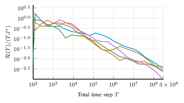
(a) Five random sample paths

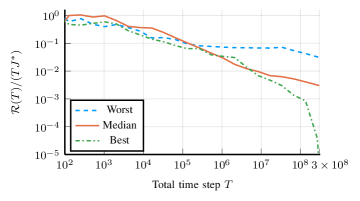
(b) Worst, median and best cases among all sample paths

Figure 2: Double-log plot of average regret against time step

An insight to behold on the performance of the proposed controller is that the circuit-breaking mechanism is triggered only finitely, and the time of the last trigger $T_{\text{nocb}}$, as stated in Corollary 5, has a super-polynomial tail. This insight is also empirically validated: among all the 10000 trials, circuit-breaking is never triggered after step $1.4\times 10^{6}$, and a histogram of $T_{\text{nocb}}$ is shown in Fig. 3, from which one can observe that the empirical distribution of $T_{\text{nocb}}$ has a fast decaying tail.

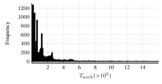
Figure 3: Histogram of $T_{\text{nocb}}$ among all sample paths

VI Conclusion

In this paper, we propose an adaptive LQR controller that can achieve $\tilde{\mathcal{O}}(\sqrt{T})$ regret almost surely. A key underlying the controller design is a circuit-breaking mechanism, which ensures the convergence of the parameter estimate, but is triggered only finitely often and hence has negligible effect on the asymptotic performance. A future direction would be extending such circuit-breaking mechanism to the partially observed LQG setting.

Yiwen Lu received his Bachelor of Engineering degree from Department of Automation, Tsinghua University in 2020. He is currently a Ph.D. candidate in Department of Automation, Tsinghua University. His research interests include adaptive and learning-based control, with applications in robotics.

Yilin Mo is an Associate Professor in the Department of Automation, Tsinghua University. He received his Ph.D. In Electrical and Computer Engineering from Carnegie Mellon University in 2012 and his Bachelor of Engineering degree from Department of Automation, Tsinghua University in 2007. Prior to his current position, he was a postdoctoral scholar at Carnegie Mellon University in 2013 and California Institute of Technology from 2013 to 2015. He held an assistant professor position in the School of Electrical and Electronic Engineering at Nanyang Technological University from 2015 to 2018. His research interests include secure control systems and networked control systems, with applications in sensor networks and power grids.

References

- [1] K. J. Astrom, “Adaptive control around 1960,” IEEE Control Systems Magazine, vol. 16, no. 3, pp. 44–49, 1996.
- [2] K. J. Åström and B. Wittenmark, “On self tuning regulators,” Automatica, vol. 9, no. 2, pp. 185–199, 1973.
- [3] A. Morse, “Global stability of parameter-adaptive control systems,” IEEE Transactions on Automatic Control, vol. 25, no. 3, pp. 433–439, 1980.
- [4] T. Lai and C.-Z. Wei, “Extended least squares and their applications to adaptive control and prediction in linear systems,” IEEE Transactions on Automatic Control, vol. 31, no. 10, pp. 898–906, 1986.
- [5] Y. Abbasi-Yadkori, D. Pál, and C. Szepesvári, “Online least squares estimation with self-normalized processes: An application to bandit problems,” arXiv preprint arXiv:1102.2670, 2011.
- [6] M. Abeille and A. Lazaric, “Improved regret bounds for thompson sampling in linear quadratic control problems,” in International Conference on Machine Learning. PMLR, 2018, pp. 1–9.
- [7] A. Cohen, T. Koren, and Y. Mansour, “Learning linear-quadratic regulators efficiently with only regret,” in International Conference on Machine Learning. PMLR, 2019, pp. 1300–1309.
- [8] S. Dean, H. Mania, N. Matni, B. Recht, and S. Tu, “Regret bounds for robust adaptive control of the linear quadratic regulator,” Advances in Neural Information Processing Systems, vol. 31, 2018.
- [9] M. Simchowitz and D. Foster, “Naive exploration is optimal for online lqr,” in International Conference on Machine Learning. PMLR, 2020, pp. 8937–8948.
- [10] M. K. S. Faradonbeh, A. Tewari, and G. Michailidis, “On adaptive linear–quadratic regulators,” Automatica, vol. 117, p. 108982, 2020.
- [11] F. Wang and L. Janson, “Exact asymptotics for linear quadratic adaptive control.” J. Mach. Learn. Res., vol. 22, pp. 265–1, 2021.
- [12] M. K. S. Faradonbeh, A. Tewari, and G. Michailidis, “Finite-time adaptive stabilization of linear systems,” IEEE Transactions on Automatic Control, vol. 64, no. 8, pp. 3498–3505, 2018.
- [13] L. Guo, “Self-convergence of weighted least-squares with applications to stochastic adaptive control,” IEEE transactions on automatic control, vol. 41, no. 1, pp. 79–89, 1996.
- [14] H. Lin and P. J. Antsaklis, “Stability and stabilizability of switched linear systems: a survey of recent results,” IEEE Transactions on Automatic control, vol. 54, no. 2, pp. 308–322, 2009.
- [15] L. Guo and H. Chen, “Convergence rate of an els-based adaptive tracker,” System Sciece and Mathematical Sciences, vol. 1, no. 2, p. 131, 1988.
- [16] H. Mania, S. Tu, and B. Recht, “Certainty equivalence is efficient for linear quadratic control,” Advances in Neural Information Processing Systems, vol. 32, 2019.
- [17] Y. Lu and Y. Mo, “Ensuring the safety of uncertified linear state-feedback controllers via switching,” arXiv preprint arXiv:2205.08817, 2022.
- [18] B. Laurent and P. Massart, “Adaptive estimation of a quadratic functional by model selection,” Annals of Statistics, pp. 1302–1338, 2000.
- [19] K. Azuma, “Weighted sums of certain dependent random variables,” Tohoku Mathematical Journal, Second Series, vol. 19, no. 3, pp. 357–367, 1967.
- [20] M. Simchowitz, H. Mania, S. Tu, M. I. Jordan, and B. Recht, “Learning without mixing: Towards a sharp analysis of linear system identification,” in Conference On Learning Theory. PMLR, 2018, pp. 439–473.
- [21] J. J. Downs and E. F. Vogel, “A plant-wide industrial process control problem,” Computers & chemical engineering, vol. 17, no. 3, pp. 245–255, 1993.
- [22] H. Liu, Y. Mo, J. Yan, L. Xie, and K. H. Johansson, “An online approach to physical watermark design,” IEEE Transactions on Automatic Control, vol. 65, no. 9, pp. 3895–3902, 2020.