Abstract

The Higgs mass is not protected by any symmetry in the Standard Model. Hence, the self-energy corrections to the Higgs mass become large due to the quadratic divergence terms. Veltman condition (V.C.) ensures that the coefficient of the quadratic divergent term either vanishes or becomes negligible. The non-observation of new physics has pushed the new physics scale to be larger than 1 TeV, making it impossible to satisfy the Veltman condition in the Standard Model without very large fine-tuning. Many attempts are made to satisfy the V.C. in Beyond Standard Model theories, but the V.C. is hard to achieve at a very large scale ($\Lambda$). Alternatively, it is possible that the new physics appears much above the Electroweak scale, and the effect of the new physics is observed in terms of the Wilson coefficients of the Standard Model Effective Field Theory (SMEFT) operators. The V.C. can be addressed in the SMEFT framework. In this paper, some specific new physics scenarios are considered at a very large scale. Below that scale, the effect of the new physics is observed as Beyond Standard Model Effective Field Theory (BSM-EFT). We particularly study the type-II seesaw model with the complex scalar triplet ($Y=1$) in the context of V.C. We found that this particular model is the minimal model to generate all SMEFT operators that appear in V.C. and satisfies V.C. We also examine the model parameter dependence of the Wilson coefficients in detail and show how the cancellation of the Wilson coefficients is highly dependent on some specific values of the model parameters.

1 Introduction

The smallness of the observed Higgs mass is confirmed by the experiments  [1, 2] at the Large Hadron Collider (LHC). However, in the Standard Model (SM) of particle physics, the scalar mass (mass of Higgs boson) is not protected by any symmetry. Hence, if SM is valid up to a large scale, Planck scale, the Higgs mass suffers from quadratic divergence ($\sim\Lambda^{2}$). To ensure that the mass of the Higgs boson is small, one has to consider a very large fine-tuning in the SM. A way to ensure that the Higgs mass does not get large correction at a higher scale is coined as Veltman condition (V.C.) [3]. V.C. checks if the sum of all quadratically divergent terms coming from the self-energy diagrams of the Higgs boson is either zero or very small. However, experiments such as the Large Hadron Collider (LHC) is pushing the New Physics (NP) scale towards $>1$ TeV, thus Veltman condition is not possible to satisfy in the SM, as it demands $\Lambda$ to be less than 760 GeV [4].

Simple extensions of SM have been studied in the literature [5, 6, 7, 8, 9, 4, 10, 11, 12], where the V.C. is valid but only in some regions of parameter space. Overall, there are two main concerns in these models: (1) These theories encounter different problems at a large scale, such as the potential becomes unstable leading to the invalidity of the theory beyond that scale, (2) The non-observation of the Beyond Standard Model (BSM) particles has pushed their masses above TeV scale [13].

One may assume that SM is valid up to a certain scale ($\Lambda$) and above that scale, some unknown symmetry appears to protect the Higgs mass, then the Higgs mass can be stabilized and the fine-tuning problem can be addressed. For example, in the Composite Higgs Scenario [14], where the Higgs is dissolved in higher degrees of freedom above the symmetry breaking scale or in Supersymmetric theories [15], where the bosonic and fermionic degrees of freedom cancel out exactly – the Higgs mass is maintained to be finite and small. These theories also can not avoid a certain amount of fine-tuning [16, 17] coming from several sources. However, experiments are yet to confirm the existence of these theories.

These observations raise the question that what if the new physics lies at a very large scale. In such a scenario, SM can emerge as an Effective Field Theory (SMEFT) [18] by integrating out the dynamics of the larger theory. The information of the heavy particles appearing in the loop is absorbed in the higher dimensional operators in the Effective Field Theory (EFT) and the theory is invariant under SM symmetries. Ref [19] has shown that the V.C. can be satisfied in the SMEFT framework by including the higher dimensional operators and their Wilson coefficients. Only a few of the operators are relevant to the V.C. and they play a major role in satisfying the V.C.

In this paper, we take one step forward and ask this question what if the theory at a very high scale ($\Lambda$) includes specific type of BSM scenarios? and how that affects the V.C.? We adopt the Beyond Standard Model Effective Field theory (BSM-EFT) [20] approach, which has been studied previously in Ref [20, 21, 22, 23, 24, 25, 26, 27]. In BSM-EFT the Lagrangian becomes invariant under the particular BSM model in consideration. The motivation to study the V.C. in the BSM-EFT framework is twofold. 1) We can specifically check how many SMEFT operators are allowed by the model. 2) As the Wilson coefficients can be expressed in terms of the model parameters, the sign of the W.C., which is crucial to obtain V.C., comes naturally. For calculation of the SMEFT operators we choose WARSAW basis [28, 29].

We begin with simple BSM scenarios (in BSM-SMEFT) such as scalar singlets, doublets and triplets (real or complex) and found that V.C. can be satisfied in all these models. We also found that the complex scalar triplet model with $Y=1$ is the minimal model (with only of one type of BSM particle) where it is possible to generate all the SMEFT operators that contributes to the V.C. In Section 4 we discuss more on this . Moreover, this particular model is well motivated in literature from other aspects as well: 1) Neutrino mass generation through the see-saw mechanism [30], 2) type-II Leptogenesis scenario [31] 3) Enhancement of the $h\rightarrow\gamma\gamma$ branching ratio [32] etc, among many other[33, 34, 35].

In Section 2, we show how the V.C. depends on the SMEFT operators in the WARSAW basis [28]. In Section 3, we discuss some specific models in the BSM-EFT scenarios, and express the Wilson coefficients of $Y=1$ complex scalar triplet model in terms of the model parameters. In Section 4, we show how V.C. is achieved by the exact cancellation of the Wilson coefficients at different scale. We also interpret the result in terms of the model parameter space. Then in Section 5, we conclude.

2 SMEFT operators and Veltman Condition

The physical mass of the Higgs in the Standard Model can be written in terms of the bare mass term $m_{h}(0)$ and the higher-order self-energy corrections:

$$m^{2}_{h}=m^{2}_{h}(0)+\delta m^{2}_{h}=m^{2}_{h}(0)+\text{Log Div. Term + Quadratic Div. Term + Finite terms},$$ (1)

where the assumption is that the SM is valid up to the scale $\Lambda$ and the correction terms are coming from the loop diagrams involving scalars, fermions and bosons in the loop. The $d=4$ potential in the Standard Model in terms of Higgs doublet ($H$) is

$$V(H)=-m_{H}^{2}H^{\dagger}H+\lambda(H^{\dagger}H)^{2}.$$ (2)

This leads to the correction to the higgs mass and the quadratic divergent contribution can be expressed as,

$$(\delta m_{h}^{2})_{\rm SM} = \frac{\Lambda^{2}}{16\pi^{2}}\left(6\lambda+\frac{9}{4}g_{W}^{2}+\frac{3}{4}g_{Y}^{2}-6y_{t}^{2}\right),$$ (3)

where, $g_{Y}$ and $g_{W}$ are the $U(1)_{Y}$ and $SU(2)_{L}$ gauge couplings respectively and $g_{t}=2m_{t}/v$ is the top quark Yukawa coupling. Here we neglect the couplings of the lighter quarks and $\Lambda$ is the cut-off scale. The Veltman condition (V.C.) demands that $\delta m_{h}^{2}\sim 0$ or at least controllably small. With the observed Higgs mass at 125 GeV, the condition to make $\delta m_{h}\sim 0$ demands $\Lambda<760$ GeV, which is already ruled out by LHC. One way to solve this problem is to introduce new particles, which can contribute in the loops and soften the fine-tuning by ensuring exact cancellation or partial as we have already discussed in the introduction.

A popular way to address this problem is to consider the effects of the higher dimensional operators in the EFT framework. Let us assume that the New Physics (NP) exists at a very high scale $\Lambda$. The effect of NP can be integrated out at $\Lambda$ and this will effectively give us SM, plus some effective operators involving only the SM fields. This is known as the Standard Model Effective Field Theory (SMEFT) [18]. The Lagrangian, which incorporates dimension six SMEFT operators in addition to the Standard Model dimension four operators, can be expressed as,

$$\mathcal{L}=\sum_{i}\mathcal{C}_{4i}\mathcal{Q}_{4i}+\frac{1}{\Lambda^{2}}\sum_{i}\mathcal{C}_{6i}\mathcal{Q}_{6i}.$$ (4)

In contrast to $\mathcal{C}_{4i}$, which is the only function of the parameters linked to the degrees of freedom in the Standard Model, $\mathcal{C}_{6i}$ are the Wilson coefficients, which are functions of the integrated out dynamics at $\Lambda$. These operators can be expanded at any choice of basis, for example, HISZ basis [36, 37], Warsaw basis [28, 29], SILH basis [38] etc. The set of dimension six operators that involves Higgs in Warsaw basis are:

$$\mathcal{Q}_{H}=(H^{\dagger}H)^{3},\,\,\ \mathcal{Q}_{HD}=(H^{\dagger}\mathcal{D}_{\mu}H)^{\ast}(H^{\dagger}\mathcal{D}^{\mu}H),\,\,\ \mathcal{Q}_{H\square}=(H^{\dagger}H)\square(H^{\dagger}H)\$$

$$\mathcal{Q}_{HB}=(H^{\dagger}H)B_{\mu\nu}B^{\mu\nu},\,\,\ \mathcal{Q}_{HW}=(H^{\dagger}H)W_{\mu\nu}^{a}W^{a,\mu\nu},\,\,\ \mathcal{Q}_{GG}=(H^{\dagger}H)G^{A}_{\mu\nu}G^{A,\mu\nu}\$$

$$\mathcal{Q}_{HWB}=(H^{\dagger}\tau_{a}H)B^{\mu\nu}W^{a}_{\mu\nu}$$ (5)

It can be shown that the last operator, $\mathcal{Q}_{HWB}$ does not contribute Higgs self-energy correction[19]. The first operator, $\mathcal{Q}_{H}$ will also not contribute at one-loop level as the Higgs does not develop a vev at $\Lambda$. There can be the appearance of the operators involving the gluons of the form $\mathcal{Q}_{GG}=(H^{\dagger}H)G^{A}_{\mu\nu}G^{A,\mu\nu}$. However, while considering BSM-EFT framework with heavy scalars, this operator does not contribute as scalars do not carry any color charge. Note that, these operators can be written in any basis, for example Ref [19] choose the HISZ basis. We choose the Warsaw basis because it is self consistent at one loop [29, 39] and easier to check the running of the Wilson coefficients in Warsaw basis.

The correction to the Higgs mass from the higher order terms in the Lagrangian is given by

$$(\delta m_{h}^{2})_{\rm total} = \frac{\Lambda^{2}}{16\pi^{2}}\sum_{i}f_{i}(\mathcal{C}_{4i},\mathcal{C}_{6i})+\frac{\Lambda^{2}}{(16\pi^{2})^{2}}\sum_{i}g_{i}(\mathcal{C}_{4i},\mathcal{C}_{6i})$$ (6)

Here $f_{i}$ and $g_{i}$ are one loop and two loop correction to the Higgs mass. The V.C., $\delta m_{h}^{2}\sim 0$ translates into

$$f(\mathcal{C}_{4i},\mathcal{C}_{6i}),g(\mathcal{C}_{4i},\mathcal{C}_{6i})\sim 0$$ (7)

if loop contributions are considered separately. The coefficients, $\mathcal{C}_{4i}$ and $\mathcal{C}_{6i}$ are function of $\Lambda$ and the BSM model parameters. Hence Eq:6 can be written in terms of the SM and higher dimension operators contribution as,

$$(\delta m_{h}^{2})_{\rm total}\equiv(\delta m_{h}^{2})_{\rm SM}\big{(}f_{i}(\mathcal{C}_{4i}),g_{i}(\mathcal{C}_{4i})\big{)}+(\delta m_{h}^{2})_{\rm HO}\big{(}f_{i}(\mathcal{C}_{6i}),g_{i}(\mathcal{C}_{6i})\big{)}$$ (8)

Also, it has been shown in Ref [19] that at $d\geq 8$, the SMEFT operators are not able to produce any $\Lambda^{6}$ divergence, which will produce any effective $\Lambda^{2}$ divergence while calculating the self-energy correction of Higgs mass. There are studies in the literature, where the V.C in terms of EFT has been studied in detail [19, 40, 41]. In particular it has been shown in Ref: [19] that it is possible to satisfy the V.C for appropriate values and sign of the Wilson coefficients at large $\Lambda$.

3 BSM-EFT with Complex Scalar Triplet

In the above section, we saw that only four operators in the WARSAW basis are involved in the V.C. Now, we assume that the new physics at a large scale follow certain symmetries of a BSM model which effectively produces SM as an EFT. It has been already shown in literature how some BSM extensions [5, 6, 7, 8, 9, 4, 10, 11, 12] address the V.C. In this paper we consider them to appear at a large scale and dictate the underlying symmetry of the EFT.

In this BSM-EFT framework, these 4 operators may or may not be possible to generate at one loop, depending on the underlying symmetry of the model at scale $\Lambda$. In Table: 1, we present if these 4 operators can be generated at one loop in some simple BSM-EFT cases with additional scalar(s) or not . For the calculation, we have implemented the Lagrangian of each model in CoDEx [42, 43] and generated the Wilson coefficients. .

Model	Quantum No	$\mathcal{Q}_{HD}$	$\mathcal{Q}_{HB}$	$\mathcal{Q}_{HW}$	$\mathcal{Q}_{H\square}$
Real Scalar Singlet	(1,1,0)	✓	✗	✗	✗
Real Scalar Triplet	(1,3,0)	✗	✗	✓	✓
Complex Scalar Triplet	(1,3,1)	✓	✓	✓	✓
Complex scalar doublets (2HDM)	(1,2,$\pm$1/2)	✓	✗	✓	✓
Real Scalar Singlet +	(1,1,0)	✓	✗	✓	✓
Real Scalar Triplet	(1,3,0)
Complex Scalar Triplet +	(1,3,1)	✓	✓	✓	✓
Complex Scalar Doublet	(1,2,1/2)

Table 1: SMEFT operators in WARSAW basis in different BSM-EFT scenarios.

Among all popular models, we have found that BSM-EFT with complex scalar triplet is the minimal model where all four Wilson coefficients are generated at one loop. In other models, the number of operators is less than four except for the model with complex scalar triplet with the additional doublet. In 2HDM scenario and real scalar singlet + triplet model, only three operators can be generated, whereas, in the complex scalar singlet model, only 2 operators are generated. The real scalar singlet model generates only one operator. All this models, with four or less number of operators satisfies the V.C. But, in is intuitive to see that the parameter space of the W.C.s is more constrained in a model which generates less than four of EFT Operators. Hence, we chose to study the complex scalar triplet model in detail as the minimal model (with only one type of BSM particle) along with other motivations as mentioned in the Introduction.

Let us consider that beyond the scale $\Lambda$, there exists a heavy complex triplet, $\Delta$, with weak hypercharge $Y=1$. The most general renormalizable tree-level scalar potential of such a model is given by

$$V(H,\Delta) = -m_{H}^{2}\left(H^{\dagger}H\right)+M^{2}\mathrm{Tr}\left[\Delta^{\dagger}\Delta\right]+\left(\mu_{\Delta}H^{T}i\sigma^{2}\Delta^{+}H+h.c\right)+\lambda\left(H^{\dagger}H\right)^{2}+\lambda_{1}\left(H^{\dagger}H\right)\mathrm{Tr}\left[\Delta^{\dagger}\Delta\right]$$

$$+ \lambda_{2}\left(\mathrm{Tr}[\Delta^{\dagger}\Delta]\right)^{2}+\lambda_{3}\mathrm{Tr}\left[(\Delta^{\dagger}\Delta)^{2}\right]+\lambda_{4}\left(H^{\dagger}\Delta\Delta^{\dagger}H\right).$$ (9)

The extra Yukawa term for neutrino mass generation is,

$$\mathcal{L}_{Y} = y_{\Delta}\ell^{T}iCi\sigma^{2}\Delta\ell+h.c.$$ (10)

Here the trilinear coupling $\mu_{\Delta}$ can be taken as positive by absorbing its phase into $H$ and $\Delta$. The total Lagrangian is,

$$\mathcal{L}=\mathcal{L}_{Y}-V(H,\Delta),$$ (11)

The details of this model is summarized in ‘Model Description’ section of the Appendix.

We explicitly show the expansion of the dimension six operators (as listed in Eq:2), in the ‘Calculation’ section of the Appendix. The Higgs mass correction in terms of W.C.s is WARSAW basis is given by,

$$(\delta m_{h}^{2})_{\rm BSM} = \frac{\Lambda^{2}}{16\pi^{2}}\Big{(}-3\mathcal{C}_{HD}+12\mathcal{C}_{H\square}+9\mathcal{C}_{HW}+3\mathcal{C}_{HB}\Big{)}\$$ (12)

$$+ \frac{\Lambda^{2}}{(16\pi^{2})^{2}}\left(54\mathcal{C}_{H}-\frac{9}{2}(g_{Y}^{2}+3g_{W}^{2})\mathcal{C}_{HD}+108g_{W}^{2}\mathcal{C}_{HW}\right).$$

The total correction to the Higgs mass is,

$$\delta m_{h}^{2}=(\delta m_{h}^{2})_{\rm SM}+(\delta m_{h}^{2})_{\rm BSM}.$$ (13)

The Wilson coefficients appearing in one loop contribution in $(\delta m_{h}^{2})_{\rm BSM}$ can be expressed in terms of the model parameters as:

$$\mathcal{C}_{HD} = -\frac{g_{Y}^{4}}{320\pi^{2}}+\frac{4\mu_{\Delta}^{2}}{M^{2}}-\frac{\lambda_{4}^{2}}{24\pi^{2}}+\frac{11g_{Y}^{2}\mu_{\Delta}^{2}}{24\pi^{2}M^{2}}-\frac{8\mu_{\Delta}^{4}}{3\pi^{2}M^{4}}+\frac{\lambda_{4}\mu_{\Delta}^{2}}{6\pi^{2}M^{2}}+\frac{3\lambda\mu_{\Delta}^{2}}{8\pi^{2}M^{2}}$$ (14)

$$\mathcal{C}_{H\square} = -\frac{g_{W}^{4}}{1920\pi^{2}}+\frac{2\mu_{\Delta}^{2}}{M^{2}}-\frac{\lambda_{1}^{2}}{16\pi^{2}}-\frac{\lambda_{1}\lambda_{4}}{16\pi^{2}}-\frac{\lambda_{4}^{2}}{192\pi^{2}}-\frac{g_{W}^{2}\mu_{\Delta}^{2}}{96\pi^{2}M^{2}}+\$$ (15)

$$+ \frac{11g_{Y}^{2}\mu_{\Delta}^{2}}{96\pi^{2}M^{2}}-\frac{49\mu_{\Delta}^{4}}{12\pi^{2}M^{4}}+\frac{\lambda_{1}\mu_{\Delta}^{2}}{8\pi^{2}M^{2}}+\frac{\lambda_{4}\mu_{\Delta}^{2}}{48\pi^{2}M^{2}}+\frac{3\lambda\mu_{\Delta}^{2}}{4\pi^{2}M^{2}}$$

$$\mathcal{C}_{HB} = \frac{g_{Y}^{2}\lambda_{1}}{32\pi^{2}}+\frac{g_{Y}^{2}\lambda_{4}}{64\pi^{2}}+\frac{11g_{Y}^{2}\mu_{\Delta}^{2}}{64\pi^{2}M^{2}}$$ (16)

$$\mathcal{C}_{HW} = \frac{g_{W}^{2}\lambda_{1}}{48\pi^{2}}+\frac{g_{W}^{2}\lambda_{4}}{96\pi^{2}}+\frac{25g_{W}^{2}\mu_{\Delta}^{2}}{192\pi^{2}M^{2}}.$$ (17)

Here, $M$ is the mass of the heavy triplet. For the theory to be valid, it is sufficient to assume that $M$ is greater than $\Lambda$. We assume the order of magnitude to be the same for $M$ and $\Lambda$ in our calculation as a limiting scenario. For $M>>\Lambda$, the W.C.s will obtain smaller values.

4 Result

In order to satisfy the Veltman condition, we consider the one loop correction to the Higgs mass ($\delta m_{h}^{2}$) and fix two benchmark scenarios at $\Lambda=100$ TeV and $\Lambda=10^{6}$ TeV. Then we figure out the model parameter space of $\lambda_{1}$ and $\lambda_{4}$, for which the quadratic divergence in $\delta m_{h}^{2}$ cancels out exactly. The SM input parameters: $g_{W}$, $y_{t}$, $g_{Y}$ and $\lambda$ are determined at $\Lambda$ by solving the two loop Renormalized Group Equation (RGE)’s. $\lambda_{1}$ and $\lambda_{4}$ are varied in such a way that the Wilson coefficients obey the perturbative limit and the running of the Wilson coefficients from $\Lambda$ to the Electroweak scale are smooth. The values of the tree level couplings ($\lambda$ and $\mu_{H}$) also shift due to the higher dimensional operators. The parameter $\lambda$ can not be more than $O(1)$ and this puts an upper limit on the quantity $\frac{\mu_{\Delta}^{2}}{2M^{2}}<O(1)$, where $\mu_{\Delta}=\frac{\sqrt{2}v_{\Delta}M^{2}}{v_{H}^{2}}$, in the limit of large scalar triplet mass. Also, precision measurements have set the value of the $\rho$ parameter to be in the range $1.00038\pm 0.00020$ (ref). This constrains the vev of the triplet ($\Delta$) to be less than $2.56$ GeV[47].

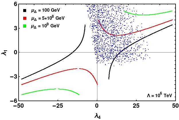
Figure 1: Variation of $\lambda_{1}$ and $\lambda_{4}$ with $\mu_{\Delta}$ at two benchmark values of $\Lambda$. V.C. is satisfied over the lines. The blue points show the allowed region when the full theory with Triplet is bounded from below and satisfies perturbative unitarity conditions.

In Fig: 1 we show the parameter space of $\lambda_{1}$ and $\lambda_{4}$ which satisfies the V.C. We found that both positive and negative values of $\lambda_{1}$ and $\lambda_{4}$ satisfy V.C. The green line represents the highest possible value of $\mu_{\Delta}$, which comes from the constraint $\frac{\mu_{\Delta}^{2}}{2M^{2}}\sim O(1)$. The nature of these plots is highly dependent on the values of $\mu_{\Delta}$, because the Wilson coefficients have $(\mu_{\Delta}/M)^{2}$ and $(\mu_{\Delta}/M)^{4}$ dependence with additional suppression of $1/16\pi^{2}$. The sign of the W.C’s come naturally from the fact that they are determined in terms of the model parameters $\lambda_{1}$, $\lambda_{4}$ and $\mu_{\Delta}$, which we allow to vary freely with the above mentioned constraints. We found that the V.C. is satisfied even if $\Lambda$ is very large ($10^{6}$ TeV). It is also essential to check whether the full theory with the Triplet scalar is well behaved above $\Lambda$. For that we have considered the vacuum stability, bounded from below and unitarity conditions [45, 46] and the blue points in Fig: 1 satisfy these conditions. We have found that the positive values of $\lambda_{1}$ and $\lambda_{4}$ are largely preferred for the full theory with the Triplet to be well behaved. Hence V.C can be satisfied in a constrained region where the full theory with the triplet obeys stability and unitarity condition. The $\lambda_{1}$ and $\lambda_{4}$ parameter space remains mostly unchanged at large $\Lambda$ because the Wilson coefficients do not change much with $\Lambda$ (shown later). Although, a slight variation in the parameter space is present due to the running of SM parameters. The cancellation in the V.C is dependent on the precision of the input parameters, which is also the source of negligible amount of fine tuning.

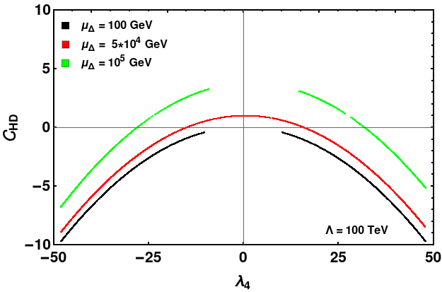
Figure 2: Variation of the Wilson coefficients with model parameter $\lambda_{4}$ when V.C. is satisfied.

In Fig: 2, we show the variation of the Wilson coefficients with the model parameter $\lambda_{4}$ at 100 TeV. The corresponding value(s) of $\lambda_{1}$ can be inferred form Fig: 1. The Wilson coefficients show similar behavior at the other benchmark scenario. For Wilson coefficients $\mathcal{C}_{HD}$ and $\mathcal{C}_{H\Box}$, negative values are more preferred, whereas, for $\mathcal{C}_{HW}$ and $\mathcal{C}_{HB}$, both positive and negative values are allowed . However, when $\lambda_{4}$ is negative, almost all coefficients are negative, except for some values of the $\mathcal{C}_{HD}$ and $\mathcal{C}_{H\Box}$. Again, when $\lambda_{4}$ is positive, $\mathcal{C}_{HW}$ and $\mathcal{C}_{HB}$ are always positive but $\mathcal{C}_{HD}$ and $\mathcal{C}_{H\Box}$ are mostly negative except for some values as shown in Fig: 2. Thus, it is visible that the cancellation among the Wilson coefficients is not ad-hoc, but is controlled by the model parameters. We have checked the V.C n=by considering the two loop contribution to Higgs mass correction as well but due to the extra suppression by ($1/16\pi^{2}$), the effect is not visible.

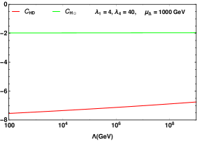
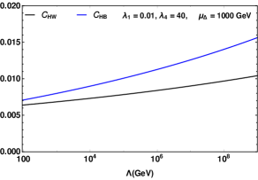
Figure 3: Running of the Wilson coefficients from $\Lambda=10^{6}$ TeV to the cut-off scale for one set of model parameters. We have kept the value of $\mu_{\Delta}$ to be fixed at $1$ TeV.

We have also checked the running of the Wilson coefficients from the effective scale $\Lambda$ to the Electroweak scale. We show the running of the Wilson coefficients in Fig: 3 for a particular choice of the model parameters, $\lambda_{1}=4.0$ and $\lambda_{4}=40$. This particular choice of parameter represents the maximum possible value of these parameters. We found that the values of these W.C.s do not change much and also the sign of the W.C.s do not change in the running. The conclusion remains the same for other allowed values of $\lambda_{1}$ and $\lambda_{4}$ that satisfy the V.C. The values of W.C.s ($C_{i}(1\rm TeV)^{2}/\Lambda^{2}$) are highly constrained at the EW scale [48] from various low energy experiments. The values of the W.C.s that satisfy the V.C., as shown in Fig: 2, Fig: 3, lie within the current experimental bounds.

5 Conclusion

The Veltman condition can not be satisfied within the framework of the Standard Model because of significant quadratic divergences to the Higgs self-energy correction if the cutoff scale $\Lambda$ is $\sim 1$ TeV or higher. In addition to the dimension four operators from the Standard Model, we have also included dimension six operators whose contributions to the Higgs mass correction results from integrating out the heavy triplet scalar with hypercharge. We show how the quadratic divergence of the Higgs self-energy vanishes in this particular model due to the cancellation among the SM parameters and the Wilson coefficients.

We have shown the relevant SMEFT operators which contribute to the V.C and found agreement with Ref. [19]. The W.C. of the operators are expressed in terms of the model parameters of the complex scalar triplet model. Hence, in this study the sign of the Wilson coefficients are not ad-hoc, it is driven by the larger theory, which is a heavy triplet scalar in our case. We found that this model generates all four operators that appear in the V.C., allowing more parameter space to the W.C.s compared to the other models, where the number of operators is less than four. However, the values of the Wilson coefficients will be different in every model, as it is controlled by the specific model parameters.

To achieve the Veltman condition, it should be noted that the contributions from two particular dimension six operators $\mathcal{Q}_{HD}$ and $\mathcal{Q}_{H\square}$ play a dominating role in canceling out the quadratic divergences. We show the parameter space where V.C is satisfied for both positive and negative values of the model parameters. We found that the V.C can be satisfied in a constrained region where the full theory with the triplet obeys stability and unitarity condition as well. We have observed that for energy scales $\Lambda$ = 100 TeV and $10^{6}$ TeV, the cancellation is almost similar. This is because the value of the W.C.s does not change much with $\Lambda$ and the insignificant amount of change appears due to the running of the SM parameters. If we introduce some relaxation in the V.C., by allowing some amount of fine-tuning, the model parameter space will surely enlarge, but it will get narrower with the increasing values of $\Lambda$. Thus, the Veltman condition can be easily satisfied in the framework of effective field theory, when a complex scalar triplet exists at a very large scale.

The study of this model as an Effective Field Theory can also be useful to revisit the Type II leptogenesis scenario, where it will be possible to generate specific dimension six terms which are dictated by the model.

Acknowledgements: JD acknowledges the Council of Scientific and Industrial Research (CSIR), Government of India, for the SRF fellowship grant with File No. 09/045(1511)/ 2017-EMR-I. JD also would like to acknowledge Research Grant No. SERB/CRG/004889/SGBKC/2022/04 of the SERB, India. The work of NK is supported by Department of Science and Technology, Government of India under the SRG grant, Grant Agreement Number SRG/2022/000363 and CRG grant with Grant Agreement Number CRG/2022/004120. We thank Prof. Anirban Kundu and Dr. Supratim Das Bakshi for the useful discussion during the preparation of the manuscript. We also thank the Referees for their valuable suggestions.

6 Appendix

Model Description:

In the type-II seesaw model, the scalar sector is extended by a complex scalar triplet($\Delta$) with hypercharge $1$, in addition to the Higgs doublet ($H$). Explicitly the fields can be written as,

$$H\left(1,2,+1/2\right)=\begin{pmatrix}\phi^{+}\\ \phi^{0}\end{pmatrix},\,\,\ \Delta\left(1,3,+1\right)=\begin{pmatrix}\Delta^{+}/\sqrt{2}&\Delta^{++}\\ \Delta^{0}&-\Delta^{+}/\sqrt{2}\end{pmatrix}$$ (18)

The numbers in the parentheses represent the charges of $SU(3)_{C}\times SU(2)_{L}\times U(1)_{Y}$ gauge group of the SM. The neutral components are:

$$\phi^{0}=\frac{v_{H}+h+i\phi_{3}}{\sqrt{2}},\,\,\ \Delta^{0}=\frac{v_{\Delta}+\delta+i\xi}{\sqrt{2}}$$ (19)

The kinetic terms corresponding to the scalar fields are given as

$$\mathcal{L}_{\rm kin}\supset(D^{\mu}H)^{\dagger}D_{\mu}H+\mathrm{Tr}\left[(D^{\mu}\Delta)^{\dagger}(D_{\mu}\Delta)\right],$$ (20)

with the covariant derivatives

$$D_{\mu}H = \partial_{\mu}H-i\frac{g_{Y}}{2}W_{\mu}^{a}\sigma^{a}H-i\frac{g_{W}}{2}B_{\mu}H,\$$

$$D_{\mu}\Delta = \partial_{\mu}\Delta-i\frac{g_{Y}}{2}\mathrm{Tr}\left[W_{\mu}^{a}\sigma^{a},\Delta\right]-i\frac{g_{W}}{2}B_{\mu}\Delta.$$ (21)

Here $\sigma^{a}$ ($a$ = 1, 2, 3) are the Pauli spin matrices and $g_{W}$ and $g_{Y}$ are the gauge couplings associated with $SU(2)_{L}$ and $U(1)_{Y}$ gauge group respectively.

Calculation:

The dimension six SMEFT operators which contribute Higgs mass correction either at one-loop or two-loop level can be written up to a total derivative as,

$$\mathcal{Q}_{HD} = (H^{+}\mathcal{D}_{\mu}H)^{\ast}(H^{+}\mathcal{D}^{\mu}H)\supset\left(\partial_{\mu}H^{\dagger}\right)HH^{\dagger}\left(\partial^{\mu}H^{\dagger}\right)+\Big{[}\frac{g_{W}^{2}}{4}\sigma^{a}\sigma^{b}H^{\dagger}W_{\mu}^{a}HH^{\dagger}W^{\mu b}H\$$

$$+ \frac{g_{Y}^{2}}{4}H^{\dagger}B_{\mu}HH^{\dagger}B^{\mu}H\Big{]}\$$

$$\mathcal{Q}_{H\square} = (H^{+}H)\square(H^{+}H)=-\partial_{\mu}\left(H^{\dagger}H\right)\partial^{\mu}\left(H^{\dagger}H\right)\$$

$$\mathcal{Q}_{HW} = (H^{+}H)W_{\mu\nu}^{a}W^{a,\mu\nu}\supset 2H^{\dagger}\Big{[}\sigma^{a}\left(\partial_{\mu}W_{\nu}^{a}\right)\sigma^{b}\left(\partial^{\mu}W^{\nu b}\right)-\sigma^{a}\left(\partial_{\mu}W_{\nu}^{a}\right)\sigma^{b}\left(\partial^{\nu}W^{\mu b}\right)\Big{]}H\ \$$

$$+ g_{W}^{2}\sigma^{a}f_{abc}\sigma^{p}f_{pqr}H^{\dagger}W_{\mu}^{b}W_{\nu}^{c}W^{\mu q}W^{\nu r}H\$$

$$\mathcal{Q}_{HB} = (H^{+}H)B_{\mu\nu}B^{\mu\nu}\supset 2H^{\dagger}\Big{[}\partial_{\mu}B_{\nu}\partial^{\mu}B^{\nu}-\partial_{\mu}B_{\nu}\partial^{\nu}B^{\mu}\Big{]}H\$$

$$\mathcal{Q}_{H} = (H^{\dagger}H)^{3}.$$ (22)

This result is given in WARSAW basis. Note that, only momentum dependent vertices can generate quartic divergence at one-loop level. Possible Feynman diagrams originating from these terms are similar to Ref.[19].

The authors in Reference [19] has performed the calculation in the HISZ basis. The transformations between the HISZ and WARSAW bases are given by,

$$\mathcal{Q}_{HD} = \mathcal{O}_{\phi,1},\,\,\ \mathcal{Q}_{H\square}=-2\mathcal{O}_{\phi,2},\,\,\,\ \mathcal{Q}_{H}=3\mathcal{O}_{\phi,3},\,\,\ \mathcal{Q}_{GG}=\mathcal{O}_{GG}\$$

$$\mathcal{Q}_{HW} = \frac{-4}{g_{W}^{2}}\mathcal{O}_{WW},\,\,\ \mathcal{Q}_{HB}=\frac{-4}{g_{Y}^{2}}\mathcal{O}_{BB},\,\,\ \mathcal{Q}_{HWB}=\frac{-4}{g_{W}g_{Y}}\mathcal{O}_{BW}.$$ (23)

A complete list of transformations can be obtained from Ref:[37]. The relevant operators in the HISZ basis, $\{\mathcal{O}_{\phi,1},\mathcal{O}_{\phi,2},\mathcal{O}_{\phi,3},\mathcal{O}_{GG},\mathcal{O}_{WW},\mathcal{O}_{BB},\mathcal{O}_{BW}\}$ are given in Ref. [19, 37]. It is worth noting that the sign of the coefficients of these SMEFT operators is not the same in both bases.

We would also like to mention that the result obtained in Eqs. 12 and 13 of Ref: [19] can be mapped exactly to our result of $\delta m_{h}^{2}$, subject to the fact that no operator in the WARSAW basis transforms to the operator $\mathcal{O}_{\phi,4}$  [49] in the HISZ basis and there is no contribution of the gluonic operator in our model. Due to the above mentioned reasons the parameter space of Wilson coefficients found in [19] (HISZ basis) and this paper (WARSAW basis) are different.

References

- [1] G. Aad et al. [ATLAS], “Observation of a new particle in the search for the Standard Model Higgs boson with the ATLAS detector at the LHC,” Phys. Lett. B 716, 1-29 (2012) doi:10.1016/j.physletb.2012.08.020 [arXiv:1207.7214 [hep-ex]].
- [2] S. Chatrchyan et al. [CMS], “Observation of a New Boson at a Mass of 125 GeV with the CMS Experiment at the LHC,” Phys. Lett. B 716, 30-61 (2012) doi:10.1016/j.physletb.2012.08.021 [arXiv:1207.7235 [hep-ex]].
- [3] M. J. G. Veltman, “The Infrared - Ultraviolet Connection,” Acta Phys. Polon. B 12, 437 (1981).
- [4] I. Chakraborty and A. Kundu, “Triplet-extended scalar sector and the naturalness problem,” Phys. Rev. D 89, no.9, 095032 (2014) doi:10.1103/PhysRevD.89.095032 [arXiv:1404.1723 [hep-ph]].
- [5] A. Kundu and S. Raychaudhuri, “Taming the scalar mass problem with a singlet higgs boson,” Phys. Rev. D 53, 4042 (1996) [arXiv:hep-ph/9410291 [hep-ph]].
- [6] A. Drozd, B. Grzadkowski and J. Wudka, “Multi-Scalar-Singlet Extension of the Standard Model - the Case for Dark Matter and an Invisible Higgs Boson,” JHEP 1204, 006 (2012) [arXiv:1112.2582 [hep-ph]].
- [7] A. Drozd, “RGE and the Fine-Tuning Problem,” arXiv:1202.0195 [hep-ph].
- [8] I. Chakraborty and A. Kundu, “Controlling the fine-tuning problem with singlet scalar dark matter,” Phys. Rev. D 87, 055015 (2013) [arXiv:1212.0394 [hep-ph]].
- [9] I. Chakraborty and A. Kundu, “Two-Higgs doublet models confront the naturalness problem,” Phys. Rev. D 90, 115017 (2014) [arXiv:1404.3038 [hep-ph]].
- [10] I. Chakraborty and A. Kundu, “Naturalness problem: Off the beaten track,” Pramana 87, no. 3, 38 (2016).
- [11] Z. Habibolahi, K. Ghorbani and P. Ghorbani, “Hierarchy problem and the vacuum stability in two-scalar dark matter model,” Phys. Rev. D 106, no.5, 055030 (2022) doi:10.1103/PhysRevD.106.055030 [arXiv:2207.12869 [hep-ph]].
- [12] R. Decker and J. Pestieau, “Lepton self-mass, Higgs scalar and heavy quark masses,” [arXiv:hep-ph/0512126 [hep-ph]].
- [13] R. L. Workman et al. [Particle Data Group], “Review of Particle Physics,” PTEP 2022, 083C01 (2022) doi:10.1093/ptep/ptac097
- [14] R. Contino, “The Higgs as a Composite Nambu-Goldstone Boson,” doi:10.1142/9789814327183_0005 [arXiv:1005.4269 [hep-ph]].
- [15] P. Fayet, “Supersymmetry and Weak, Electromagnetic and Strong Interactions,” Phys. Lett. B 64, 159 (1976) doi:10.1016/0370-2693(76)90319-1
- [16] J. Barnard, D. Murnane, M. White and A. G. Williams, “Constraining fine tuning in Composite Higgs Models with partially composite leptons,” JHEP 09, 049 (2017) doi:10.1007/JHEP09(2017)049
- [17] M. van Beekveld, S. Caron and R. Ruiz de Austri, “The current status of fine-tuning in supersymmetry,” JHEP 01, 147 (2020) doi:10.1007/JHEP01(2020)147
- [18] I. Brivio and M. Trott, “The Standard Model as an Effective Field Theory,” Phys. Rept. 793, 1-98 (2019) doi:10.1016/j.physrep.2018.11.002 [arXiv:1706.08945 [hep-ph]].
- [19] A. Biswas, A. Kundu and P. Mondal, “Hierarchy problem and dimension-six effective operators,” Phys. Rev. D 102, no.7, 075022 (2020) doi:10.1103/PhysRevD.102.075022 [arXiv:2006.13513 [hep-ph]].
- [20] S. Adhikari, I. M. Lewis and M. Sullivan, “Beyond the Standard Model effective field theory: The singlet extended Standard Model,” Phys. Rev. D 103, no.7, 075027 (2021) doi:10.1103/PhysRevD.103.075027 [arXiv:2003.10449 [hep-ph]].
- [21] S. Karmakar and S. Rakshit, “Relaxed constraints on the heavy scalar masses in 2HDM,” Phys. Rev. D 100, no.5, 055016 (2019) doi:10.1103/PhysRevD.100.055016 [arXiv:1901.11361 [hep-ph]].
- [22] T. Alanne and F. Goertz, “Extended Dark Matter EFT,” Eur. Phys. J. C 80, no.5, 446 (2020) doi:10.1140/epjc/s10052-020-7999-2 [arXiv:1712.07626 [hep-ph]].
- [23] S. Bar-Shalom, J. Cohen, A. Soni and J. Wudka, “Phenomenology of TeV-scale scalar Leptoquarks in the EFT,” Phys. Rev. D 100, no.5, 055020 (2019) doi:10.1103/PhysRevD.100.055020 [arXiv:1812.03178 [hep-ph]].
- [24] Y. Du, X. X. Li and J. H. Yu, “Neutrino seesaw models at one-loop matching: discrimination by effective operators,” JHEP 09, 207 (2022) doi:10.1007/JHEP09(2022)207 [arXiv:2201.04646 [hep-ph]].
- [25] X. Li, D. Zhang and S. Zhou, “One-loop matching of the type-II seesaw model onto the Standard Model effective field theory,” JHEP 04, 038 (2022) doi:10.1007/JHEP04(2022)038 [arXiv:2201.05082 [hep-ph]].
- [26] D. Zhang and S. Zhou, “Complete one-loop matching of the type-I seesaw model onto the Standard Model effective field theory,” JHEP 09, 163 (2021) doi:10.1007/JHEP09(2021)163 [arXiv:2107.12133 [hep-ph]].
- [27] A. Crivellin, M. Ghezzi and M. Procura, “Effective Field Theory with Two Higgs Doublets,” JHEP 09, 160 (2016) doi:10.1007/JHEP09(2016)160 [arXiv:1608.00975 [hep-ph]].
- [28] B. Grzadkowski, M. Iskrzynski, M. Misiak and J. Rosiek, “Dimension-Six Terms in the Standard Model Lagrangian,” JHEP 10, 085 (2010) doi:10.1007/JHEP10(2010)085 [arXiv:1008.4884 [hep-ph]].
- [29] E. E. Jenkins, A. V. Manohar and M. Trott, “Renormalization Group Evolution of the Standard Model Dimension Six Operators I: Formalism and lambda Dependence,” JHEP 10, 087 (2013) doi:10.1007/JHEP10(2013)087 [arXiv:1308.2627 [hep-ph]].
-
[30]
J. Schechter and J. W. F. Valle,
“Neutrino Masses in SU(2) x U(1) Theories,”
Phys. Rev. D 22, 2227 (1980);
R. N. Mohapatra and G. Senjanovic, “Neutrino Masses and Mixings in Gauge Models with Spontaneous Parity Violation,” Phys. Rev. D 23, 165 (1981);
C. -S. Chen and C. -M. Lin, “Type II Seesaw Higgs Triplet as the inflaton for Chaotic Inflation and Leptogenesis,” Phys. Lett. B 695, 9 (2011) [arXiv:1009.5727 [hep-ph]];
A. Chaudhuri, W. Grimus and B. Mukhopadhyaya, “Doubly charged scalar decays in a type II seesaw scenario with two Higgs triplets,” JHEP 1402, 060 (2014) [arXiv:1305.5761 [hep-ph]]. -
[31]
See, e.g.
E. Ma and U. Sarkar,
“Neutrino masses and leptogenesis with heavy Higgs triplets,”
Phys. Rev. Lett. 80, 5716 (1998)
[hep-ph/9802445];
T. Hambye, E. Ma and U. Sarkar, “Supersymmetric triplet Higgs model of neutrino masses and leptogenesis,” Nucl. Phys. B 602, 23 (2001) [hep-ph/0011192];
D. Aristizabal Sierra, M. Dhen and T. Hambye, “Scalar triplet flavored leptogenesis: a systematic approach,” arXiv:1401.4347 [hep-ph]. -
[32]
A. Arhrib, R. Benbrik, M. Chabab, G. Moultaka and L. Rahili,
“ Coupling in Higgs Triplet Model,”
arXiv:1202.6621 [hep-ph];
A. G. Akeroyd and S. Moretti, “Enhancement of H to gamma gamma from doubly charged scalars in the Higgs Triplet Model,” Phys. Rev. D 86, 035015 (2012) [arXiv:1206.0535 [hep-ph]]. -
[33]
I. Gogoladze, N. Okada and Q. Shafi,
“Higgs boson mass bounds in a type II seesaw model with triplet scalars,”
Phys. Rev. D 78, 085005 (2008)
[arXiv:0802.3257 [hep-ph]];
H. E. Logan and M. -A. Roy, “Higgs couplings in a model with triplets,” Phys. Rev. D 82, 115011 (2010) [arXiv:1008.4869 [hep-ph]];
F. Arbabifar, S. Bahrami and M. Frank, “Neutral Higgs Bosons in the Higgs Triplet Model with nontrivial mixing,” Phys. Rev. D 87, 015020 (2013) [arXiv:1211.6797 [hep-ph]]. P. S. Bhupal Dev, D. K. Ghosh, N. Okada and I. Saha, “125 GeV Higgs Boson and the Type-II Seesaw Model,” JHEP 1303, 150 (2013) [Erratum-ibid. 1305, 049 (2013)] [arXiv:1301.3453]. C. Englert, E. Re and M. Spannowsky, “Triplet Higgs boson collider phenomenology after the LHC,” Phys. Rev. D 87, no. 9, 095014 (2013) [arXiv:1302.6505 [hep-ph]]; “Pinning down Higgs triplets at the LHC,” Phys. Rev. D 88, 035024 (2013) [arXiv:1306.6228 [hep-ph]]. - [34] S. Ashanujjaman, K. Ghosh and R. Sahu, “Low-mass doubly charged Higgs bosons at the LHC,” Phys. Rev. D 107, no.1, 015018 (2023) doi:10.1103/PhysRevD.107.015018 [arXiv:2211.00632 [hep-ph]].
- [35] S. Ashanujjaman and K. Ghosh, “Revisiting type-II see-saw: present limits and future prospects at LHC,” JHEP 03, 195 (2022) doi:10.1007/JHEP03(2022)195 [arXiv:2108.10952 [hep-ph]].
- [36] K. Hagiwara, T. Hatsukano, S. Ishihara and R. Szalapski, “Probing nonstandard bosonic interactions via W boson pair production at lepton colliders,” Nucl. Phys. B 496, 66-102 (1997) doi:10.1016/S0550-3213(97)00208-3 [arXiv:hep-ph/9612268 [hep-ph]].
- [37] I. Brivio, S. Bruggisser, E. Geoffray, W. Killian, M. Krämer, M. Luchmann, T. Plehn and B. Summ, “From models to SMEFT and back?,” SciPost Phys. 12, no.1, 036 (2022) doi:10.21468/SciPostPhys.12.1.036 [arXiv:2108.01094 [hep-ph]].
- [38] G. F. Giudice, C. Grojean, A. Pomarol and R. Rattazzi, “The Strongly-Interacting Light Higgs,” JHEP 06, 045 (2007) doi:10.1088/1126-6708/2007/06/045 [arXiv:hep-ph/0703164 [hep-ph]].
- [39] R. Alonso, E. E. Jenkins, A. V. Manohar and M. Trott, “Renormalization Group Evolution of the Standard Model Dimension Six Operators III: Gauge Coupling Dependence and Phenomenology,” JHEP 04, 159 (2014) doi:10.1007/JHEP04(2014)159 [arXiv:1312.2014 [hep-ph]].
- [40] G. Passarino, “Veltman, Renormalizability, Calculability,” Acta Phys. Polon. B 52, no.6-7, 533 (2021) doi:10.5506/APhysPolB.52.533 [arXiv:2104.13569 [hep-ph]].
- [41] F. Abu-Ajamieh, “Model-independent Veltman condition, naturalness and the little hierarchy problem *,” Chin. Phys. C 46, no.1, 013101 (2022) doi:10.1088/1674-1137/ac2ffa [arXiv:2101.06932 [hep-ph]].
- [42] S. Das Bakshi, J. Chakrabortty and S. K. Patra, “CoDEx: Wilson coefficient calculator connecting SMEFT to UV theory,” Eur. Phys. J. C 79, no.1, 21 (2019) doi:10.1140/epjc/s10052-018-6444-2 [arXiv:1808.04403 [hep-ph]].
- [43] Anisha, S. Das Bakshi, S. Banerjee, A. Biekötter, J. Chakrabortty, S. Kumar Patra and M. Spannowsky, “Effective limits on single scalar extensions in the light of recent LHC data,” [arXiv:2111.05876 [hep-ph]].
- [44] A. Carmona, A. Lazopoulos, P. Olgoso and J. Santiago, “Matchmakereft: automated tree-level and one-loop matching,” SciPost Phys. 12, no.6, 198 (2022) doi:10.21468/SciPostPhys.12.6.198 [arXiv:2112.10787 [hep-ph]].
- [45] D. Das and A. Santamaria, “Updated scalar sector constraints in the Higgs triplet model,” Phys. Rev. D 94, no.1, 015015 (2016) doi:10.1103/PhysRevD.94.015015 [arXiv:1604.08099 [hep-ph]].
- [46] A. Arhrib, R. Benbrik, M. Chabab, G. Moultaka, M. C. Peyranere, L. Rahili and J. Ramadan, “The Higgs Potential in the Type II Seesaw Model,” Phys. Rev. D 84, 095005 (2011) doi:10.1103/PhysRevD.84.095005 [arXiv:1105.1925 [hep-ph]].
- [47] R. Ghosh, B. Mukhopadhyaya and U. Sarkar, “The parameter and the CDF W-mass anomaly: observations on the role of scalar triplets,” [arXiv:2205.05041 [hep-ph]].
- [48] J. Ellis, M. Madigan, K. Mimasu, V. Sanz and T. You, “Top, Higgs, Diboson and Electroweak Fit to the Standard Model Effective Field Theory,” JHEP 04, 279 (2021) doi:10.1007/JHEP04(2021)279 [arXiv:2012.02779 [hep-ph]].
- [49] S. Willenbrock and C. Zhang, “Effective Field Theory Beyond the Standard Model,” Ann. Rev. Nucl. Part. Sci. 64, 83-100 (2014) doi:10.1146/annurev-nucl-102313-025623 [arXiv:1401.0470 [hep-ph]].