Toward Accurate Measurement of Property-Dependent Galaxy Clustering:
II. Tests of the Smoothed Density-corrected ${V_{\rm max}}$ Method

Abstract

We present a smoothed density-corrected ${V_{\rm max}}$ technique for building a random catalog for property-dependent galaxy clustering estimation. This approach is essentially based on the density-corrected ${V_{\rm max}}$ method of Cole (2011), with three improvements to the original method. To validate the improved method, we generate two sets of flux-limited samples from two independent mock catalogs with different $k+e$ corrections. By comparing the two-point correlation functions, our results demonstrate that the random catalog created by the smoothed density-corrected ${V_{\rm max}}$ approach provides a more accurate and precise measurement for both sets of mock samples than the commonly used ${V_{\rm max}}$ method and redshift shuffled method. For flux-limited samples and color-dependent subsamples, the accuracy for the projected correlation function is well constrained within $1\%$ on the scale of $0.07{h^{-1}\rm Mpc}-30{h^{-1}\rm Mpc}$. The accuracy of the redshift-space correlation function is less than $2\%$ as well. Currently, it is the only approach that holds promise for achieving the goal of high-accuracy clustering measures for next-generation surveys.

1 Introduction

Over the last couple of decades, the successful observation of galaxy redshift surveys (e.g., Two Degree Field Galaxy Redshift Survey (2dFGRS) Colless et al. 2003; the Sloan Digital Sky Survey (SDSS) York et al. 2000; the Baryon Oscillation SpectroscopicSurvey (BOSS) Eisenstein et al. 2011; the VIMOS Public Extragalactic Redshift Survey (VIPERS) Garilli et al. 2012) have enabled significant progress toward our understanding of galaxy formation and evolution (Madgwick et al., 2003; Berlind et al., 2006; Guo et al., 2011, 2018; Zu et al., 2021), the galaxy-halo connection (Jing et al., 1998; Yang et al., 2003, 2008, 2012; Zheng et al., 2005, 2009; Vale & Ostriker, 2004; Alam et al., 2021a; Wechsler & Tinker, 2018; Behroozi et al., 2019), and the nature of gravity and dark energy ( Peacock et al. 2001; Weinberg et al. 2013; Samushia et al. 2013; Alam et al. 2021b and reference therein). In the upcoming years, next-generation surveys, such as the Dark Energy Spectroscopic Instrument (DESI; Levi et al. 2013; DESI Collaboration et al. 2016a, b), the Legacy Survey of Space and Time (LSST; LSST Dark Energy Science Collaboration 2012), the space mission Euclid (Amendola et al., 2013) and CSST (Cao et al., 2018; Gong et al., 2019), will map the 3D galaxy distribution in an unprecedentedly volume, leading to about an order of magnitude more extragalactic spectroscopic redshifts than those that SDSS, BOSS and eBOSS have achieved (Zarrouk et al., 2021; Yuan et al., 2022b; Myers et al., 2022; Schlegel et al., 2022). Massive amounts of data from deeper in the sky will provide new insights into the physics of galaxy formation, as well as the nature of dark matter and dark energy (Hahn et al., 2022). Galaxy two-point statistics, being one of the most fundamental tools, will continue to play a crucial role in future data analysis (Valluri et al., 2022; Amin et al., 2022), as they have in the past (Zehavi et al., 2011; Nuza et al., 2013; Skibba et al., 2014; Samushia et al., 2014; Guo et al., 2014; Planck Collaboration et al., 2016; Shi et al., 2018). Due to different systematics, it is still difficult to reliably measure small-scale property-dependent galaxy clustering at the present time. These systematics include redshift-dependent completeness, the missing galaxies in observations (Reid et al., 2016; Bianchi & Percival, 2017; Bianchi & Verde, 2020), the incorrect estimation of the radial selection model (Ross et al., 2012; Yang et al., 2020), among others (Breton & de la Torre, 2021; Farrow et al., 2021; Merz et al., 2021). Fortunately, the coming big data will considerably reduce random errors in clustering determination, but to reach the high accuracy of clustering analysis required by the next generation surveys, we must eliminate systematic errors in measurement (Beutler et al., 2014; Reid et al., 2016; Glanville et al., 2021; Dávila-Kurbán et al., 2021). In this study, the systematic bias produced by the radial selection model is investigated in greater detail.

To measure the galaxy two-point correlation function (hereafter 2PCF), we must build a random catalog with the same angular and radial selection functions as the observed sample, but with a random distribution in the observed space (Davis & Peebles, 1983; Hamilton, 1993). The angular selection function is easy to obtain from observation, but the radial selection function is difficult to estimate accurately. As the sample has a fixed number density and the redshift distribution of a random catalog is straightforward to construct (Tegmark et al., 2004), previous works often use a volume-limited sample for clustering analysis (Norberg et al., 2002; Zehavi et al., 2002, 2005, 2011; McBride et al., 2011; Shi et al., 2016; Mohammad et al., 2018). However, due to the need of excluding a substantial number of galaxies, the statistical precision of the clustering measurement is reduced (Zehavi et al., 2005; Xu et al., 2016). Alternatively, a flux-limited sample may optimize the utilization of observed galaxies, but since its radial selection function $\phi(z)$ changes with redshift, it is not easy to build the redshifts of random galaxies for a flux-limited sample unless we know the galaxy luminosity function (LF) $\Phi(M_{\rm r})$ (Loveday et al., 2015; Karademir et al., 2021).

The radial selection function for the flux-limited sample has been recovered using a number of ways. For instance, the smooth spline fit approach utilizes a spline model to fit the redshift distribution of a galaxy sample (Reid et al., 2010; Wang et al., 2017). The ${V_{\rm max}}$ method populates random galaxies within the maximum viewable volume of a real galaxy, which is dependent on the galaxy’s observational limitations. The redshift shuffled technique is a commonly employed alternative (Guo et al., 2013; Zu & Mandelbaum, 2015; Wang et al., 2021). This approach chooses redshifts at random from the real galaxy sample and assigns them to the random galaxy catalog. Through clustering analysis of the VIPERS data, de la Torre et al. (2013) showed that the spline fit approach underestimates the predicted 2PCF in comparison to the ${V_{\rm max}}$ method, particularly on scales larger than $3~{}{h^{-1}\rm Mpc}$. In the BOSS systematics investigation, Ross et al. (2012) revealed that the shuffled technique had a minor bias in BAO measurement compared to the spline fit method (Ross et al., 2015). However, de Mattia & Ruhlmann-Kleider (2019) demonstrated that the shuffled approach suffers from the integral constraint effect when measuring the power spectrum. Using mocks from a high-resolution simulation, Yang et al. (2020) (hereafter Paper I) found that both the redshift shuffled technique and ${V_{\rm max}}$ method underestimate galaxy clustering by 30% and 20%, respectively, on scales $\gtrsim~{}10{h^{-1}\rm Mpc}$ for flux-limited samples. Consequently, as long as we continue to use the aforementioned radial selection methods to construct the redshifts for random catalogs for a flux-limited sample, our clustering measurement will contain an unavoidable systematic deviation from the true galaxy clustering.

Cole (2011) proposes a density-corrected ${V_{\rm max}}$ technique for concurrently estimating LF and generating a random catalog for a flux-limited sample. Unlike the conventional ${V_{\rm max}}$ method, this technique can successfully eliminate density fluctuations. In Cole (2011), they examine the radial distribution of random galaxies, which is in excellent agreement with the input galaxy sample. This method has been employed to determine property-dependent galaxy clustering (Farrow et al., 2015) and clustering analysis (de la Torre et al., 2017; Pezzotta et al., 2017; Loveday et al., 2018; Johnston et al., 2021). However, its clustering measurement performance has not been assessed. The purpose of this study is to test the Cole (2011) technique for clustering measurements using mock data. In addition, some modifications are made to the original approach in order to improve its measurement accuracy.

This paper is structured as follows. In Section 2, we review the Cole (2011) method and introduce the smoothed density-corrected ${V_{\rm max}}$ method. The construction of mock galaxy catalogs is detailed in Section 3. We present the testing results of the correlation functions in Section 4. In Section 5, we assess the smoothed density-corrected ${V_{\rm max}}$ method and discuss the potential sources of uncertainty in estimates. We conclude the paper in Section 6.

2 Smoothed Density-corrected ${V_{\rm max}}$ Method

To address the difficulty of recovering the radial selection function of a property-dependent galaxy sample, Cole (2011) developed a density-corrected ${V_{\rm max}}$ approach for galaxy clustering estimates. This section starts with a briefly overview of the Cole (2011) technique. Following that, we detail the improvements to the original Cole (2011) methodology, which we call the smoothed density-corrected ${V_{\rm max}}$ method.

2.1 Cole (2011) Method

On the basis of the standard ${V_{\rm max}}$ approach, Cole (2011) presented a weighted ${V_{\rm max}}$ method based on a joint stepwise maximum likelihood method, which effectively eliminates the influence of density fluctuation. In this method, a density-weighted maximum volume ${V^{\rm DC}_{\rm max}}$  is defined, which is the normal ${V_{\rm max}}$ weighted by the estimated galaxy overdensities $\Delta(z)$ and the LF density evolution $P(z)$. They further define a weight as

$$w_{\alpha}\equiv\frac{V_{\alpha,\rm max}}{V^{\rm DC}_{\alpha,\rm max}+\mu V_{\alpha,\rm max}},$$ (1)

where $V_{\alpha,\rm max}$ and $V^{\rm DC}_{\alpha,\rm max}$ are the normal ${V_{\rm max}}$ and density-corrected ${V_{\rm max}}$ for the $\alpha$th galaxy in the observed sample. $\mu$ is a Lagrange multiplier providing constraints with $\langle\frac{V_{\alpha,\rm max}}{V^{\rm DC}_{\alpha,\rm max}+\mu V_{\alpha,\rm max}}\rangle=1$ when estimating LF for the galaxy sample. Lastly, a random catalog can be created by replicating individual galaxies $n_{\alpha}=nw_{\alpha}$ times and distributing them at random across the $V_{\alpha,\rm max}$ volume. Note that, unlike the standard ${V_{\rm max}}$ approach, $n_{\alpha}$ is no longer the same for all galaxies and the selection rate of random galaxies is adjusted by weight $w_{\alpha}$. The brightness of the galaxy may be over- or underrepresented in the observed sample as a result of the density variation in the ${V_{\rm max}}$ volume being appropriately compensated by the weight $w_{\alpha}$. By comparing the output redshift distribution to that of the input galaxy sample, Cole (2011) proved that the random catalog created by this density-weighted ${V_{\rm max}}$ technique could recover the genuine galaxy selection function. While this approach has not yet been tested on galaxy clustering using mock galaxy catalog, it remains to be validated using mocks.

2.2 Smoothed Density-corrected ${V_{\rm max}}$ Method

Before testing the Cole (2011) method, we perform three modifications to the original public code . The original algorithm is only applicable to galaxy sample with a single faint flux cut, but by adding a $z_{\rm min}$ estimate, our first update makes the code applicable to a generic double flux-cut sample . The maximum(minimum) redshifts $z_{\rm max(min)}$ in our updated code is same as Paper I and are determined as follows:

$$z_{\rm max} = \mathtt{min}[z_{\rm mag,max},~{}z_{\rm sample,max}],$$ (2)

$$z_{\rm min} = \mathtt{max}[z_{\rm mag,min},~{}z_{\rm sample,min}],$$ (3)

where $z_{\rm sample,max(min)}$ is the redshift limits of the galaxy sample, and $z_{\rm mag,max(min)}$ is derived by

$$m_{\rm faint} = M+{\rm DM}(z_{\rm mag,max})+k(z)-E(z),$$ (4)

$$m_{\rm bright} = M+{\rm DM}(z_{\rm mag,min})+k(z)-E(z),$$ (5)

where the flux limits are set by apparent magnitude $m_{\rm bright(faint)}$, $M$ is the absolute magnitude, the distance modulus is ${\rm DM}=5{\rm log}_{10}(d_{\rm L})+25-5{\rm log}_{10}h$, $k(z)$ is the $k$ correction, and $E(z)$ is the luminosity evolution correction ($e$ correction). Our second code improvement is the $k$ correction. In the original code, the $k$ correction is performed for all galaxies depending on the input function $k(z)$, which hinders the method’s ability to apply to a real galaxy sample whose $k$ correction is dependent not just on redshift but also on galaxy properties (e.g., color). We modify the code to take a $k$(z,color) model as input, allowing $k$ correction to be conducted on individual galaxies based on their redshifts and colors. This makes the technique more applicable to observable galaxies. Following the aforementioned modifications, the output cloned random catalog from the updated algorithm is basically consistent with the genuine radial distribution of the galaxy number density $n_{\rm true}(z)$. However, there are small fluctuations in the output radial distribution that have a considerable influence on the final clustering estimate. Our final modification to the algorithm is to smooth the radial distribution of the output cloned random galaxies. In the smooth procedure, we begin by generating a histogram of comoving distance $d$ for the random galaxies. We set a bin size of $\Delta d=5{h^{-1}\rm Mpc}$, and $N(d)_{\rm hist}$ represents the number of random galaxies in each bin. Second, we employ a convolution operator to smooth the histogram as $N^{\rm s}_{\rm hist}=[N_{\rm hist}\ast\Delta_{\rm smooth}]$, where $\Delta_{\rm smooth}=5$ is the smoothed box size in 1D and $N^{\rm s}_{\rm hist}$ is the smoothed radial distribution of random galaxies. Final redshifts for random galaxies are generated based on the profile of $N^{\rm s}_{\rm hist}$ that has been smoothed. In Section 4.2, we will observe that our modifications enhance the clustering measurement accuracy significantly.

Farrow et al. (2015) recently developed the Cole (2011) technique to quantify the property-dependent galaxy clustering of GAMA II data (Driver et al., 2011; Liske et al., 2015). They found that the Cole (2011) technique yields a redshift distribution that is too broad for cloned random galaxies, which may be the result of luminosity evolution. To mitigate this unanticipated impact, Farrow et al. (2015) developed a Gaussian window function to restrict the redshift distribution of the cloned galaxies. In the first place, the mock galaxy catalogs that we construct in this study resemble the low redshift SDSS data, as opposed to the GAMA data, which encompass a relatively broad redshift range of 0$\sim$0.5. In our mock galaxies, luminosity evolution is expected to have negligible effects. Second, our first adjustment to the $z_{\rm min}$ calculation narrows the distribution of cloned random galaxies. Our test findings in Section 4.2 will demonstrate that the smoothed density-corrected ${V_{\rm max}}$ approach is adequate for obtaining accurate galaxy clustering determination.

3 Mock Galaxy Catalogs

In this section, we describe the construction of mock galaxy catalogs for a robust test of the smoothed density-corrected ${V_{\rm max}}$ approach on clustering estimation. We build two sets of mock samples, one with simple $k+e$ corrections and the other with complex $k+e$ corrections for galaxies.

The first group of mock galaxy catalogs is created in a manner similar to that used in Paper I. For the halo catalog, we adopt the $\rm WMAP\_3072\_600$ cosmological $N$-body simulation from the CosmicGrowth simulation suite (Jing, 2019). This simulation starts at redshift 144 with $3072^{3}$ particles evolving in a $600~{}{h^{-1}\rm Mpc}$ cube box. The simulation assumes a standard flat $\Lambda\rm CDM$ cosmology with $\{\Omega_{m}=0.268,~{}\Omega_{b}=0.045,~{}\sigma_{8}=0.83,~{}n_{s}=0.968\}$ and $h=H_{0}/(100\,{\rm km}\,\mathrm{s}^{-1}\mathrm{Mpc}^{-1})=0.71$, which are compatible with the Nine-Year Wilkinson Microwave Anisotropy Probe (WMAP 9) observations (Hinshaw et al., 2013; Bennett et al., 2013). This simulation has a mass resolution of $5.54\times 10^{8}~{}h^{-1}\rm M_{\sun}$. To identify halos for each output snapshot, the friends-of-friends technique is used with a linking length of 0.2 in units of the mean particle separation (Davis et al., 1985). The Hierarchical Bound-Tracing technique is used to find subhalos and their merger histories. In this study, the snapshot at $z=0$ is utilized to build the halo catalog, and each halo contains at least 50 particles. The orphan halos are also maintained in the catalog (Yang et al., 2019).

We use the subhalo abundance matching method to establish the connection between galaxies and subhalos. Based on the galaxy’s absolute magnitude $M^{0.1}_{\rm r}$ and the peak mass $M_{\rm peak}$ of subhalos, a monotonic relationship between the cumulative number density $n(<M^{0.1}_{\rm r})=n(>M_{\rm peak})$ has been constructed (Conroy et al., 2006; Hearin et al., 2014; Wechsler & Tinker, 2018; Contreras et al., 2021). We employ the LF of the SDSS DR7 ${\tt full\_1}$ sample of the New York University Value-Added catalog (NYU-VAGC) (Blanton et al., 2001, 2003, 2005), for which the $r-$band absolute magnitude $M^{0.1}_{\rm r}$ of galaxies has been $k$ and $e$corrected to $z=0.1$. The $M_{\rm peak}$ is the maximum mass ever attained by a subhalo over its entire evolutionary history. Once a subhalo has been matched to a galaxy, its position and velocity are given to the galaxy. By periodically rotating and stacking the mock box, we generate 60 mock galaxy catalogs from the parent catalog. Random sites are assigned to the observer. The observed redshift $z_{\rm obs}$ is determined by the galaxy’s position and velocity relative to the observer. To obtain the apparent magnitude $m_{\rm r}$, the $k$ correction and $e$ correction, as described in Equations (4) and (5), must be provided. Real data processing determines these values by fitting the observed galaxy flux to a library of synthetic spectrum models, which is generally inapplicable to mock galaxies and also beyond the scope of this work. For the sake of simplicity, we consider two simple $k+e$correction cases here. In the first case, no $k+e$ corrections are applied to the mock galaxies. In the second case, we suppose that all galaxies follow a simple $k+e$ correction model. For the $k$correction, we take the model of Smith et al. (2017):

$$k^{0.1}(z)=\sum^{4}_{i=0}A_{i}(z-0.1)^{4-i}.$$ (6)

Smith et al. (2017) fit the above fourth-order polynomial to individual GAMA galaxies, where $A_{i}$ is the polynomial’s fitting coefficient (McNaught-Roberts et al., 2014). There are seven color-dependent $k(z)$ models (see the section below) and we adopt the $(g-r)^{0.1}_{\rm med}=0.603$ model with the following fitting coefficients: $A_{0}=-3.428$, $A_{1}=9.478$, $A_{2}=-2.703$, and $A_{3}=0.7646$. For the $e$ correction, we use the SDSS model (Blanton, 2006) :

$$E(z)=q_{0}[1+q_{1}(z-z_{0}))](z-z_{0}),$$ (7)

where $z_{0}=0.1$ is the zero-point redshift for evolution correction, $q_{0}=2$ denotes the evolution of magnitude per redshift, $q_{1}=-1$ is the nonlinear parameter in redshift evolution. After applying the $k+e$ corrections to the mock galaxies, our final samples are constructed as follows. For each mock catalog in each $k+e$ correction case, we first generate a flux-limited sample with flux cuts at $m_{\rm r}=[15,17]$ and a sky coverage of $\sim 5950~{}\rm deg^{2}$. The flux-limited catalog is then divided into two luminosity-dependent samples, designated LC1 with $M^{0.1}_{\rm r}=[-19,-22]$ and LC2 with $M^{0.1}_{\rm r}=[-20,-23]$. Using these selection criteria, the galaxy sample’s number density changes as a function of redshift. Figure 13 in Appendix A displays the average number density $\overline{n}(z)$ of the 60 samples for two luminosity cuts in each $k+e$ correction case. This redshift-dependent number density typically prevents us from obtaining an accurate measurement of galaxy clustering, particularly at scales $\leq 30{h^{-1}\rm Mpc}$ for flux-limited samples (Yuan et al., 2022a). In the following text, the above mock samples generated from the simulation of (Jing, 2019) are referred to as LC samples.

The second group of mock galaxy catalogs is built from the light cone catalog of Smith et al. (2017) . It is essential to assess the radial selection model using a catalog of galaxies that closely resembles the observed galaxies. The Smith et al. (2017) catalog is constructed using the MXXL simulation (Angulo et al., 2012), which assumes a $\Lambda$CDM cosmology with WMAP1 parameters $\{\Omega_{m}=0.25,~{}\sigma_{8}=0.9,~{}n_{s}=0.968,h=0.73\}$ and operates in a $3h^{-1}\rm Gpc$ box. The mass of the particle is $6.17\times 10^{9}h^{-1}\rm M_{\sun}$. Smith et al. (2017) created the light cone catalog by applying the halo occupation distribution method to link galaxies to subhalos. To assign colors to the galaxies, they utilize an enhanced redshift-dependent Skibba & Sheth (2009) model. The galaxy $k+e$ corrections in their light cone catalog are more complicated than the ones we use for the LC samples. They employ color-dependent $k$ corrections obtained from the GAMA survey for the $k$ corrections. In brief, they estimate the $k$ corrections for individual galaxies in GAMA data by fitting with equation (6), and they determine the median $k$ correction in seven evenly spaced color bins to construct seven $k-$correction models. These models are $(g-r)^{0.1}_{\rm med}=$ 0.131,0.298,0.443,0.603,0.785,0.933, and 1.067 with different polynomial coefficients. The $k(z,color)$ is then interpolated for the light cone catalog using seven median color $(g-r)^{0.1}_{\rm med}$ models based on the galaxy’s color and redshift . For the LF evolution, they employed the evolving Schechter function derived from GAMA data. In the low-redshift region $z\lesssim 0.13$, the LF of their catalog coincides with the LF of Blanton et al. (2003), which we employ for the LC samples, and in the median redshift region, the LF evolves to the GAMA LF. The luminosity(color)-dependent galaxy clusterings in Smith et al. (2017) catalog are generally consistent with the SDSS DR7 results measured by Zehavi et al. (2011) at low redshift, as well as the GAMA results measured by Farrow et al. (2015) at the median redshift. Therefore, this catalog is suitable for testing different radial selection models for property-dependent clustering measurement. We construct 10 flux-limited samples from the full-sky light cone catalog by rotating the sky, using the galaxy selection criteria ($m_{\rm r}=[15,17]$) and sky coverage ($\sim 5950~{}\rm deg^{2}$). Two luminosity-dependent galaxies, LS1 ($M^{0.1}_{\rm r}=[-19,-22]$) and LS2 ($M^{0.1}_{\rm r}=[-20,-23]$), are generated from each flux-limited sample, much as we did for the LC samples. As our sample selection resembles the SDSS DR7 data, we further divide the luminosity-dependent sample into a blue subsample and a red subsample using the color-cut equation $(g-r)^{0.1}_{\rm cut}=0.21-0.03M^{0.1}_{\rm r}$ of Zehavi et al. (2011). In the rest of this study, we refer to the mock galaxy samples built from the Smith et al. (2017) catalog as LS samples.

In summary, we generate two sets of mock samples from two simulations using the same selection criterion for galaxies. For the LC samples, flux-limited samples are constructed from 60 mocks with two absolute magnitude cuts. Two cases are considered for $k+e$ corrections: (1) there are no $k+e$ corrections; (2) all galaxies are assumed to follow a simple $k+e$ correction model. Ten LS samples are created in the same manner as the LC samples, but using a public light cone catalog. The LS samples, however, feature a color-dependent $k-$correction and a complex $e$ correction that are unknown to us. In order to examine the color-dependent clustering, the luminosity-dependent LS data are split into blue and red subsamples. We emphasize that neither the LC samples nor the LS samples are subjected to any deliberate impact (e.g., fiber collision) in order to decrease unknown systematic uncertainty in our later tests. In addition, when calculating the comoving distance from redshift, we employ the cosmological model of the simulation from which the samples are constructed, separately.

4 Testing the Smoothed Density-corrected ${V_{\rm max}}$ Method with the 2PCFs

In this section, we describe the construction of a random galaxy catalog, focusing on the radial distribution of random galaxies derived from various radial selection models. Following that, we compare the correlation functions generated by the random catalogs used in these models.

4.1 Construction of the Random Catalogs

The random catalogs are constructed as follows. For the angular distribution, we first generate a large number of random points that are uniformly dispersed across the surface of a unit sphere. For each mock sample and subsample, we extract a collection of points with the same sky coverage as the corresponding sample and subsample. We consider the positions of these points to be the angular distribution (R.A., decl.) of the random galaxies, with no angular selection effect or survey masks imposed. For the redshifts of random galaxies, the following radial selection models are used in our tests:

1. $\mathbf{n_{\rm\textbf{true}}}$ method, which generates the redshift distribution for random galaxies using the true galaxy number density $n(z)_{\rm true}$ taken from the LF of the parent mock catalog.

2. $\mathbf{V^{\rm\textbf{SDC}}_{\rm\textbf{max}}}$ method, in which redshifts for the random catalog are generated using the smoothed density-corrected ${V_{\rm max}}$ method.

3. $\mathbf{V^{\rm\textbf{DC}}_{\rm\textbf{max}}}$ method, in which the density-corrected ${V_{\rm max}}$ method of Cole (2011) is utilized, but without the smoothing procedure.

4. $\mathbf{V_{\rm\textbf{max}}}$ method, where the normal ${V_{\rm max}}$ method is adopted.

5. Shuffled method, which applies the redshift shuffled method. In this method, galaxy redshifts of the sample are randomly assigned to the random galaxies.

For LC samples, it is simple to incorporate the $k+e$ corrections into the redshift generation process. Enabling the validation of the capacity of different radial selection models to restore the true radial selection function $n(z)_{\rm true}$. Figure 1 shows a comparison between the radial distributions of a single LC sample and random catalogs generated by the aforementioned radial selection methods in the case of no $k+e$ corrections. In the left and right panels, the comparisons for LC1 and LC2 samples are presented, respectively. The second row of panels displays the deviation of random galaxy number relative to the galaxy number in each comoving distance bin, which is defined as $\Delta_{\rm g}=(n_{\rm r}-n_{\rm g})/n_{\rm g}$. The third row of panels displays the deviation of the random galaxy number of the other four techniques from the number of the $n_{\rm true}$ approach, defined as $\Delta_{\rm n_{\rm true}}=(n_{\rm r}-n_{\rm r,true})/n_{\rm r,true}$. The black histograms in the top row of panels denote the distribution of galaxies in the flux-limited samples. The radial distribution of random catalogs created by the $n_{\rm true}$ method is represented by green lines, which indicate the distribution arising from the genuine selection function. The purple-dashed line indicates the distribution produced from the ${V^{\rm DC}_{\rm max}}$ approach. We see small fluctuations in the radial distribution, which are notably clear in the bottom row of panels. These noisy fluctuations have been reduced by the smoothing process in the ${V^{\rm SDC}_{\rm max}}$ approach; as indicated by the blue solid lines, the smoothed radial distribution is in excellent agreement with the distribution predicted by the $n_{\rm true}$ method.

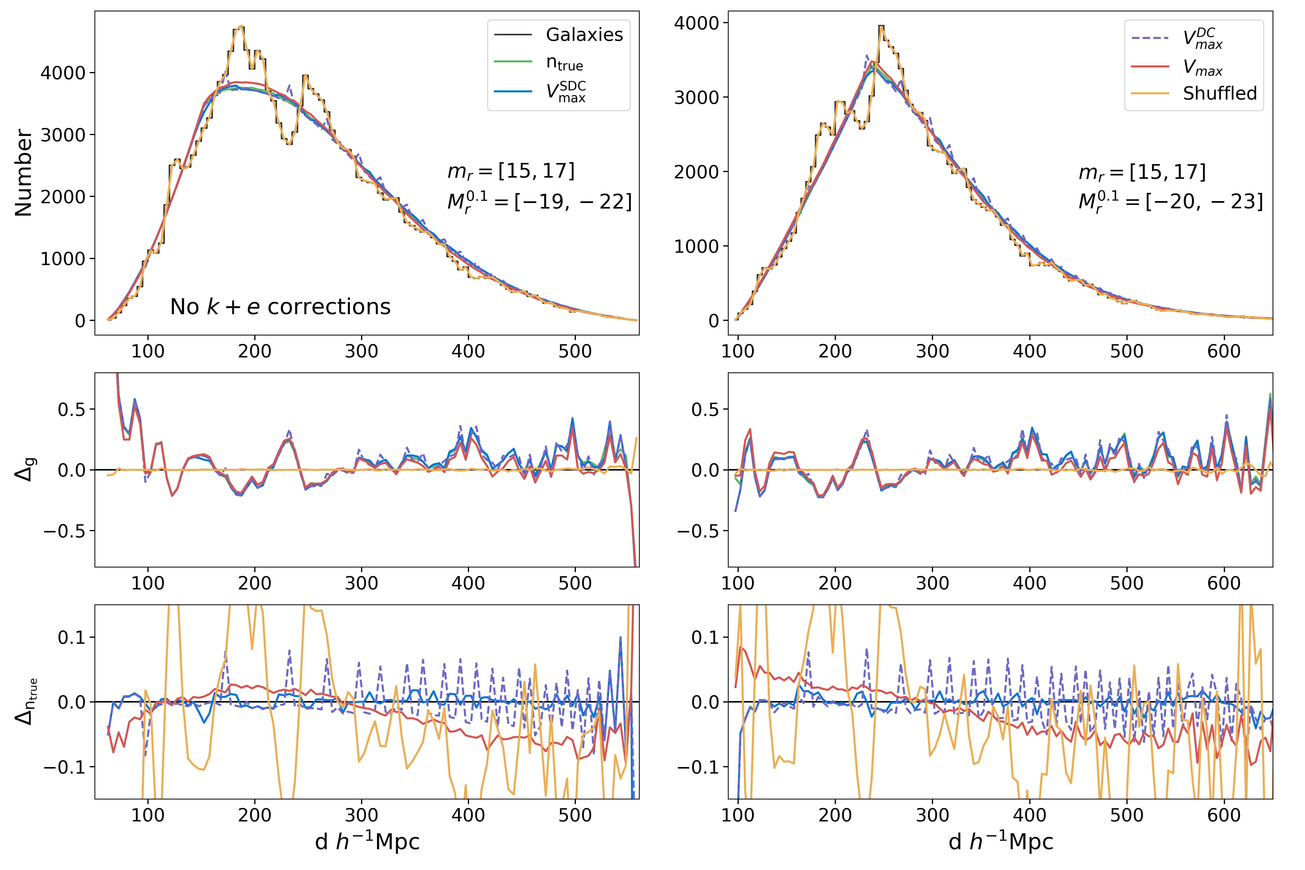
Figure 1: In the case of no $k+e$ correction, a comparison of the radial distributions of one LC sample and its corresponding random catalogs. The bin size is $\Delta d=5~{}{h^{-1}\rm Mpc}$. The LC samples have a flux cut at $m_{\rm r}=[15,17]$ and two luminosity cuts at $M^{0.1}_{\rm r}=[-19,-22]$ (left panels) and $M^{0.1}_{\rm r}=[-20,-23]$ (right panels). The black histogram denotes galaxy distribution. Random catalogs generated by the $n(z)_{\rm true}$, ${V^{\rm SDC}_{\rm max}}$, ${V^{\rm DC}_{\rm max}}$, ${V_{\rm max}}$, and shuffled methods are represented by the green, blue, purple-dashed, red, and yellow lines, respectively. The second row of panels displays the number bias $\Delta_{\rm g}$ in each bin of the random catalogs compared to the galaxies, calculated as $\Delta_{\rm g}=(n_{\rm r}-n_{\rm g})/n_{\rm g}$. The third row of panels displays the number bias of random catalogs compared to $n(z)_{\rm true}$, which is defined as $\Delta_{\rm n_{\rm true}}=(n_{\rm r}-n_{\rm r,true})/n_{\rm r,true}$.

The radial distributions from the ${V_{\rm max}}$ and the shuffled methods are represented by red and yellow lines, respectively. As shown in the bottom panels, $\Delta_{\rm n_{\rm true}}$ of the ${V_{\rm max}}$ approach exhibits a systematic bias in both luminosity-dependent LC samples as a result of the influence of large-scale structures in galaxy radial distribution. The ${V_{\rm max}}$ approach creates an excess of random galaxies near these structures; hence, the number of random galaxies in the high-redshift tail has been decreased. Figure 2 shows the same comparison as Figure 1 for LC samples with the simple $k+e$ corrections. The deviations of different approaches from the $n_{\rm true}$ method shown in the bottom panels are similar to those in Figure 1.

Figure 3 shows a comparison for the LS samples, employing the same color-coded lines as Figure 1. The left panels compare an LS1 sample, whereas the middle and right panels compare its blue and red subsamples, respectively. For the $n_{\rm true}$ method, the radial selection function derived from the LF of the light cone catalog is applied. The $k+e$ corrections are appropriately incorporated into the redshift generation process for the $n_{\rm true}$ and ${V_{\rm max}}$ methods. For the ${V^{\rm SDC}_{\rm max}}$ and ${V^{\rm DC}_{\rm max}}$ methods, the same $k-$correction models that Smith et al. (2017) performed for their light cone database are employed, which interpolate the $k$ correction from seven models based on the color and redshift of individual galaxies. The $e$ correction is also properly applied to the LS samples and their color-dependent subsamples by using the evolutionary property of the light cone catalog. The results of the comparison are generally consistent with those of the LC samples. The redshifts generated by the ${V_{\rm max}}$ technique are substantially influenced by the sample’s structures; the bias in $\Delta_{\rm n_{\rm true}}$ is greater than that of the LC samples, which reaches 20% on the high-redshift tail (red solid lines). The redshifts from the ${V^{\rm SDC}_{\rm max}}$ approach successfully mitigate this impact, resulting in a relatively small deviation in $\Delta_{\rm n_{\rm true}}$ (blue solid lines). For both the LC and LS samples, the redshifts of random catalogs obtained by the shuffled approach replicate the radial distribution of galaxies (yellow solid lines); hence, the structures are also cloned. In the following section, we will examine how galaxy clustering measurements are affected by the deviations in these radial distributions that differ from the expected distribution produced by the $n_{\rm true}$ model.

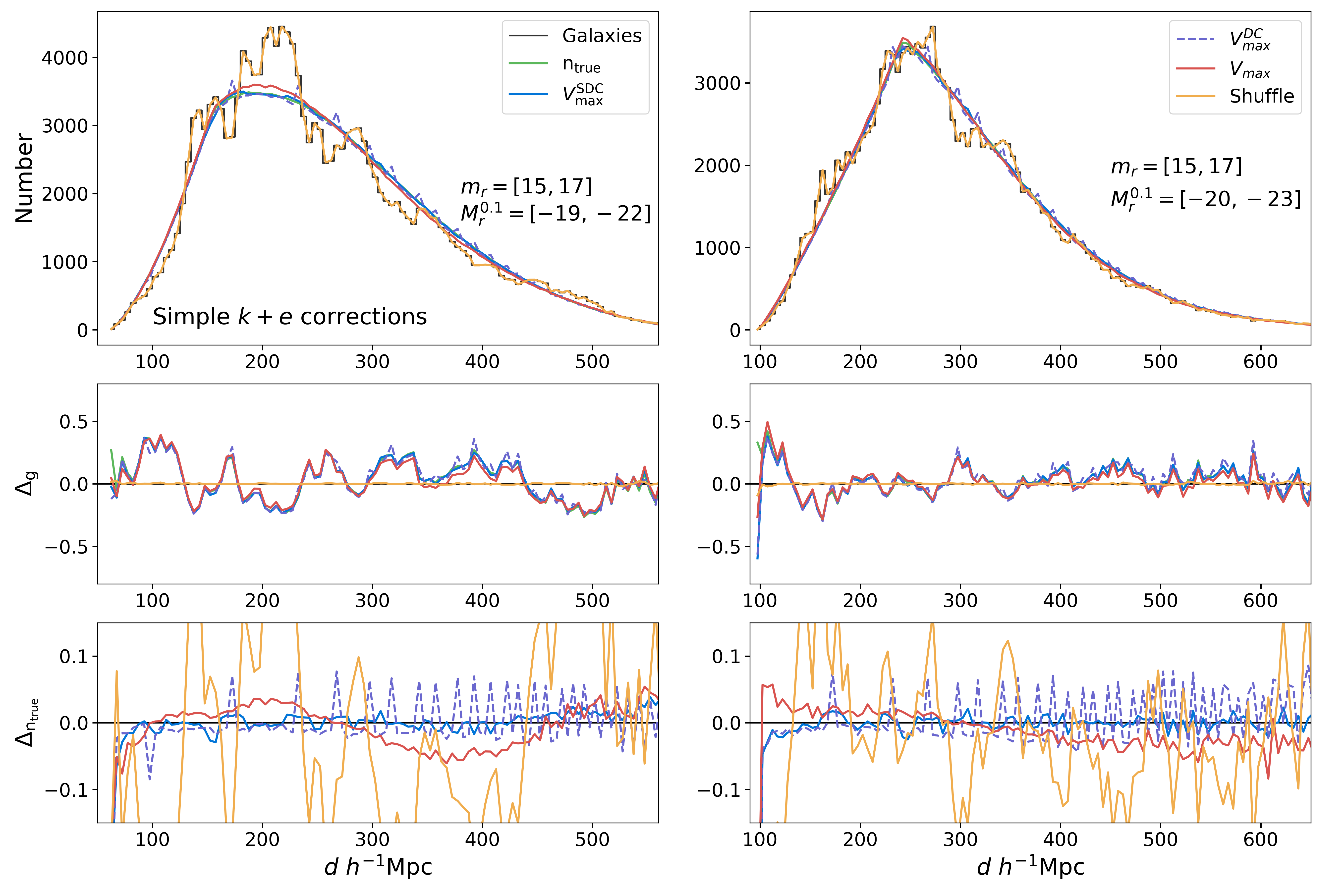
Figure 2: The same as Figure 1 but for the simple $k+e$ correction case of the LC samples.

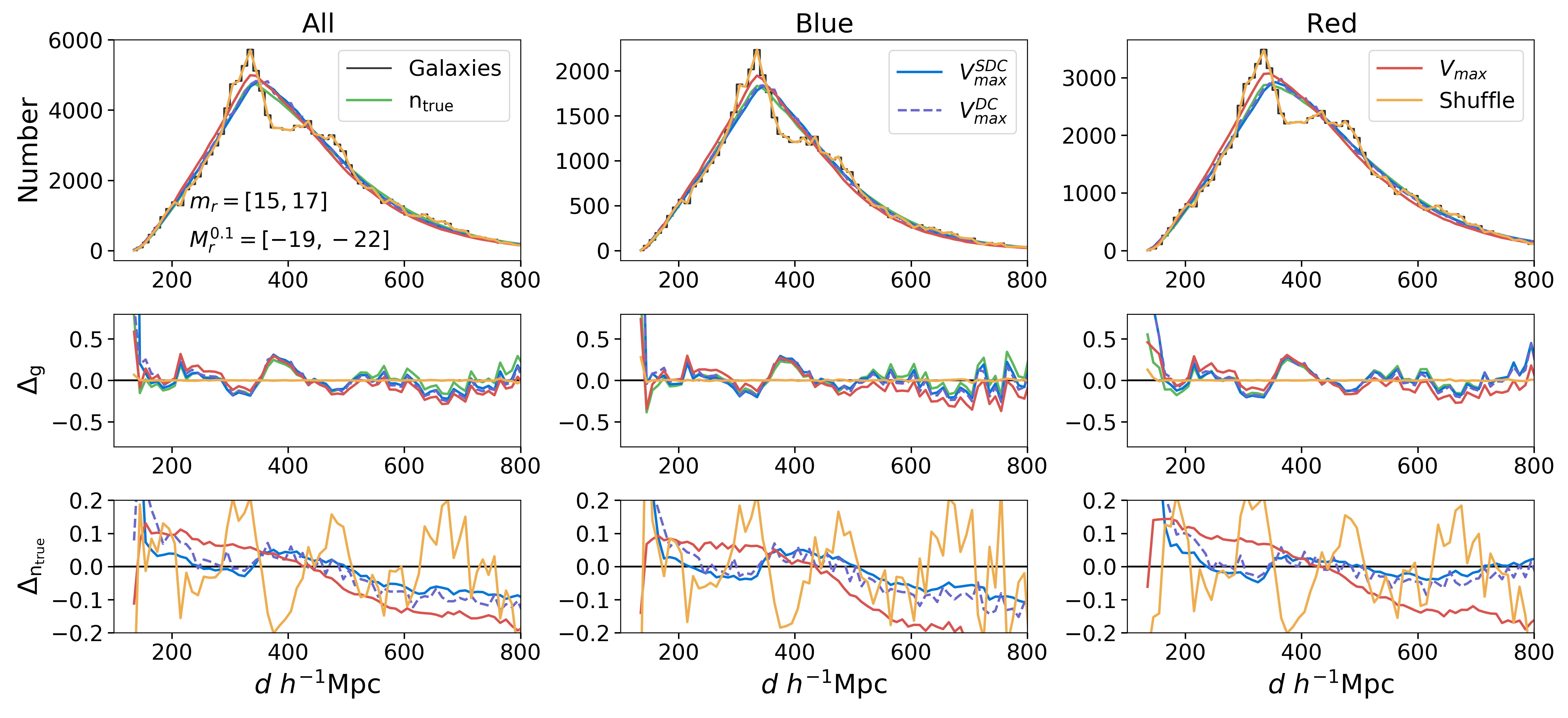
Figure 3: The same as Figure 1 but for the LS1 samples.

4.2 Comparison of the Correlation Functions

This section introduces the 2PCF estimator that we employ to measure galaxy clustering. Then, we provide a comparison of the projected 2PCFs and the redshift-space 2PCFs determined from random catalogs generated by the aforementioned radial selection methods.

4.2.1 Estimator

We measure the 2PCF in the same way as Paper I. First, we define the redshift separation vector $\bm{s}$ and the line-of-sight vector $\bm{l}$ as $\bm{s}\equiv\bm{\upsilon}_{1}-\bm{\upsilon}_{2}$ and $\bm{l}\equiv(\bm{\upsilon}_{1}+\bm{\upsilon}_{2})/2$, where $\bm{\upsilon}_{1}$ and $\bm{\upsilon}_{2}$ are redshift-space position vectors of a pair of galaxies (Hamilton, 1992; Fisher et al., 1994). Separations that are parallel ($\pi$) and perpendicular ($r_{p}$) to the line-of-sight direction are derived as

$$\pi\equiv\frac{\bm{s}\cdot\bm{l}}{|\bm{l}|},~{}~{}~{}~{}~{}~{}r^{2}_{p}\equiv\bm{s}\cdot\bm{s}-\pi^{2}.$$ (8)

We construct a grid of $\pi$ and $r_{p}$ by taking $1~{}{h^{-1}\rm Mpc}$ as the bin size for $\pi$ from 0 up to $\pi_{\rm max}=40~{}{h^{-1}\rm Mpc}$ linearly, and a bin size of $0.2$ for $r_{p}$ is adopted logarithmically in the range of [$0.01$, $40$] ${h^{-1}\rm Mpc}$. The estimator of Landy & Szalay (1993) is used to calculate the 2D correlation function as

$$\xi(r_{p},\pi)=\frac{DD-2DR+RR}{RR},$$ (9)

where $DD$, $DR$, and $RR$ are the numbers of data-data, data-random, and random-random pairs. Given $s^{2}=|\bm{s}|^{2}=r^{2}_{p}+\pi^{2}$, we derive the redshift-space correlation function $\xi(s)$. By integrating $\xi(r_{p},\pi)$ along the line-of-sight direction, we estimate the projected 2PCF (Davis & Peebles, 1983) by

$$w_{p}(r_{p})\equiv 2\int^{\infty}_{0}\xi(r_{p},\pi)~{}d\pi\approx 2\int^{\pi_{max}=40}_{0}\xi(r_{p},\pi)~{}d\pi.$$ (10)

We employ the public code $\tt{CORRFUNC}$ (Sinha & Garrison, 2019) for pair counting in this work. To reduce the shot noise on small-scale clustering, we use 50 times the number of galaxies in the random catalogs for random galaxies.

4.2.2 Comparison of Projected 2PCFs

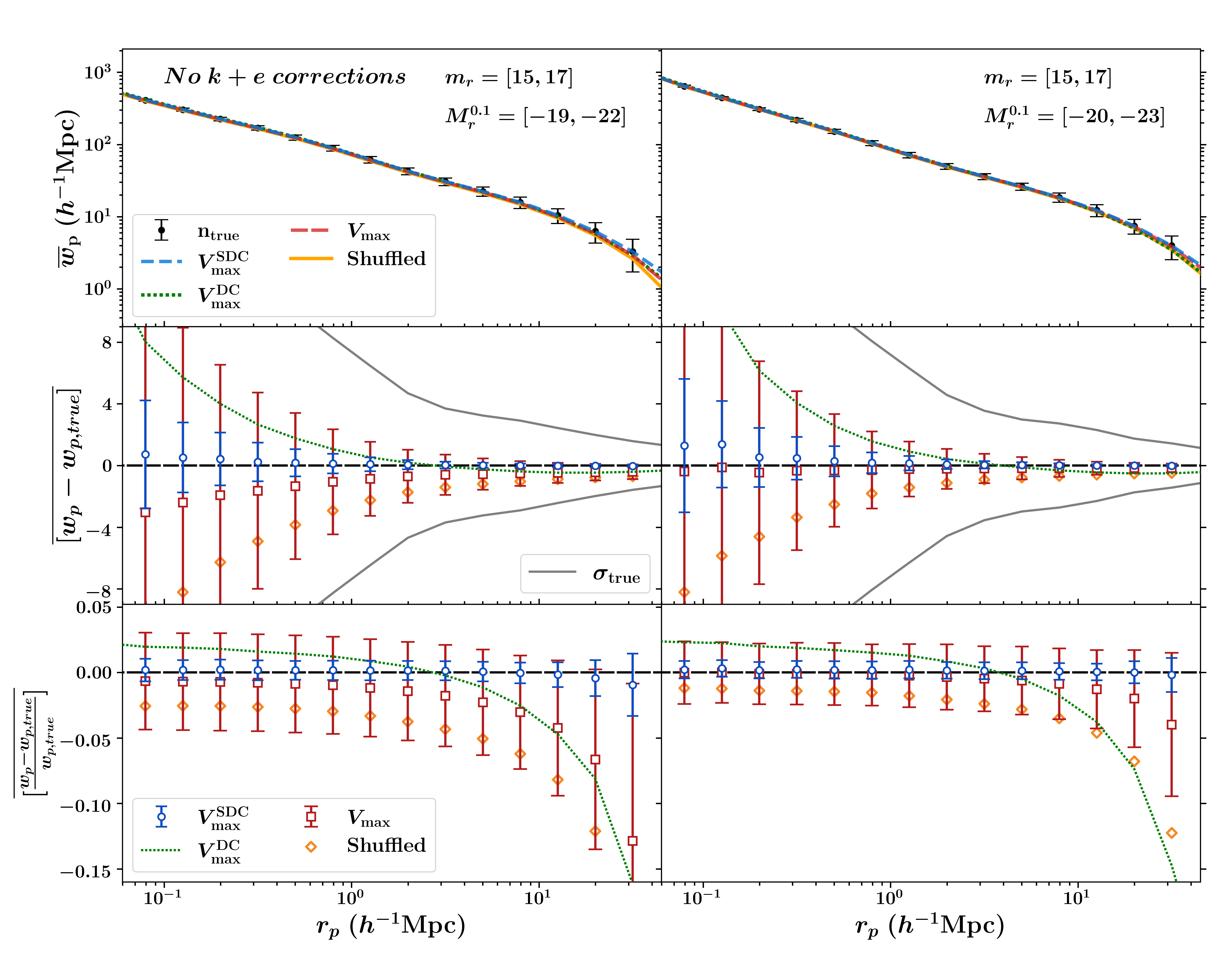
Figure 4: Top panels: The average projected correlation functions $\overline{w}_{p}$ for LC1 (left panel) and LC2 (right panel) samples in the case of no $k+e$ corrections. The LC1 samples have a flux-cut at $m_{r}=[15,17]$ and a luminosity cut at $M^{0.1}_{r}=[-19,-22]$. LC2 samples have the same flux-cut as LC1 samples but a brighter luminosity cut at $M^{0.1}_{r}=[-20,-23]$. The solid black points with error bars represent the $\overline{w}_{p,true}$ and $1\sigma$ dispersion across 60 of the LS samples utilizing random catalogs generated by the $n_{\rm true}$ approach. $\overline{w}_{p}$ of the ${V^{\rm SDC}_{\rm max}}$, ${V^{\rm DC}_{\rm max}}$, ${V_{\rm max}}$, and shuffled methods are shown by the blue-dashed lines, the green-dotted lines, the red long-dashed lines, and the orange lines, respectively. Middle panels: the average deviations from $w_{p,true}$ for various techniques of assigning redshifts to random catalogs, as determined by the $w_{p}$ of the 60 LC samples. The blue open rolls with error bars represent the mean offset and $1\sigma$ deviations of $w_{p}$ for the ${V^{\rm SDC}_{\rm max}}$ technique. The results of the ${V_{\rm max}}$ technique are displayed as open red squares with error bars. The mean offsets computed from $w_{p}$ for the ${V^{\rm DC}_{\rm max}}$ and shuffled methods are shown by green-dashed lines and yellow open diamonds, accordingly. The gray lines represent the $1\sigma$ dispersion of $w_{p,true}$ among the 60 LC samples. The horizontal-dashed black lines indicate the zero offset. Bottom panels: The average bias of $w_{p}$ relative to $w_{p,true}$ for four radial selection models, defined as $\overline{[(w_{p}-w_{p,true})/w_{p,true}]}$. The color-coded lines and symbols are identical to those in the middle panels.

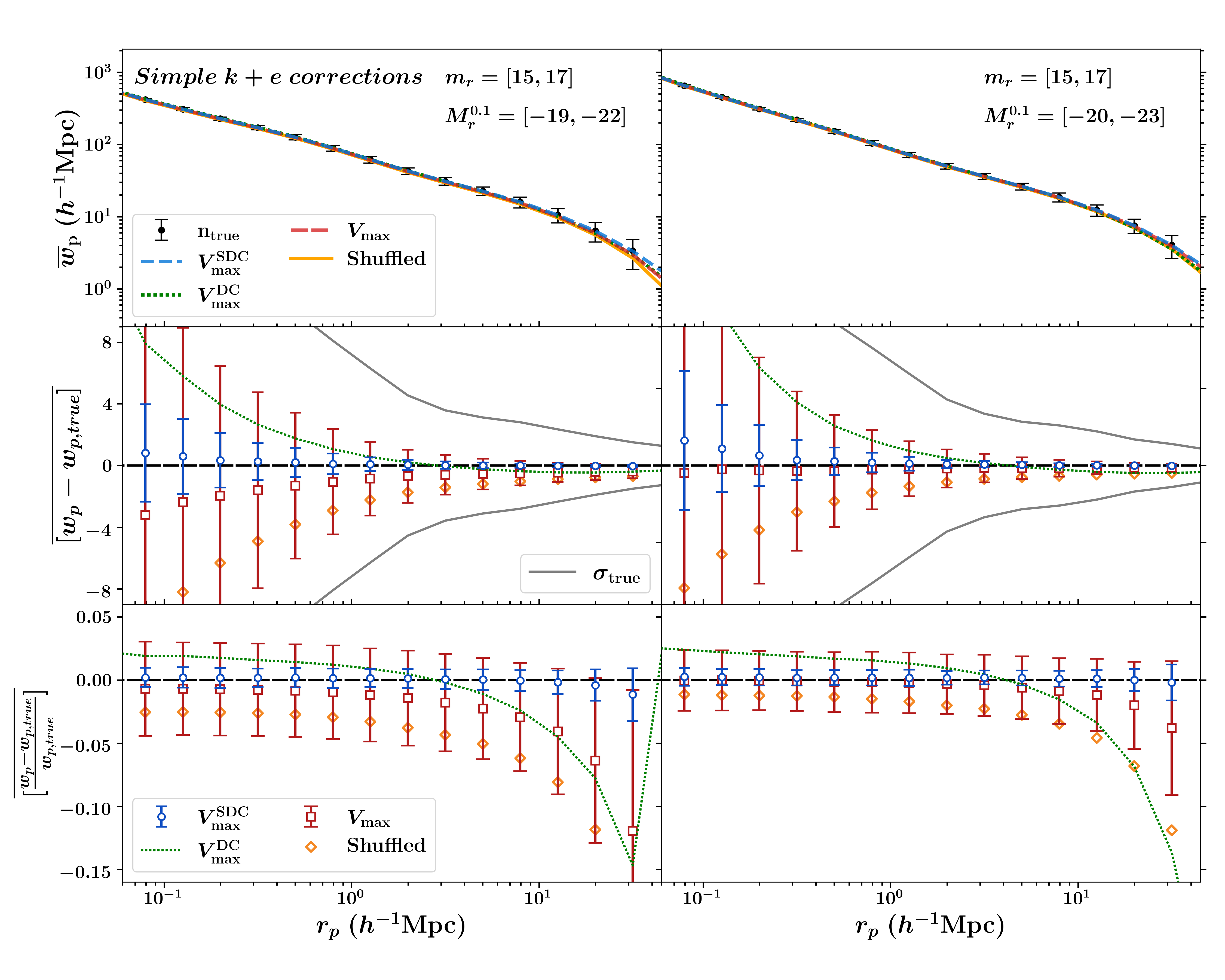
Figure 5: The same as Figure 4 but for the LC samples with simple $k+e$ corrections.

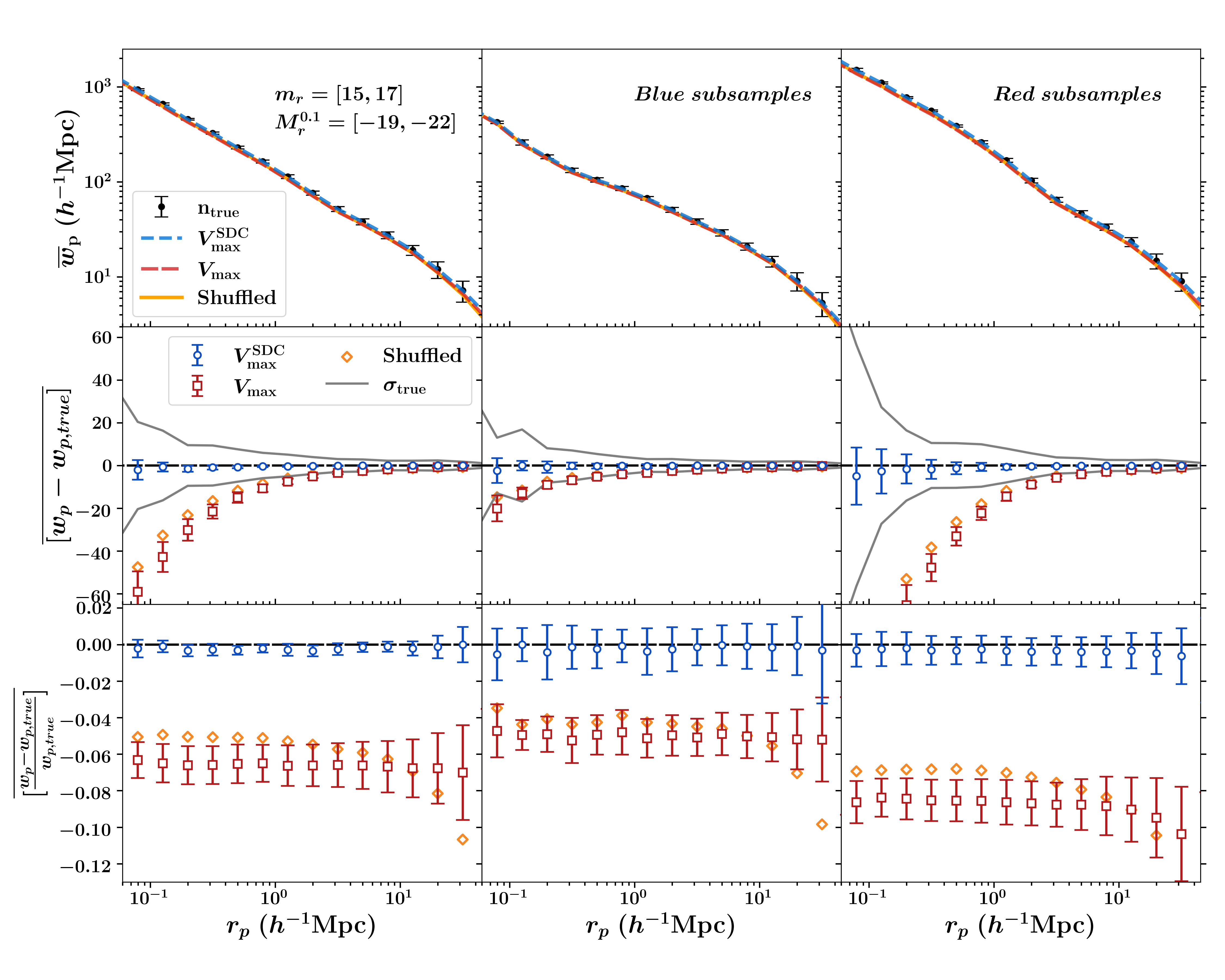
Figure 6: Similar to Figure 4: comparison of $w_{p}$ for the LS1 samples (left panels) and their blue (middle panels) and red (right panels) subsamples. The color-coded lines and symbols are identical to those in Figure 4, excluding the result of the ${V^{\rm DC}_{\rm max}}$ technique.

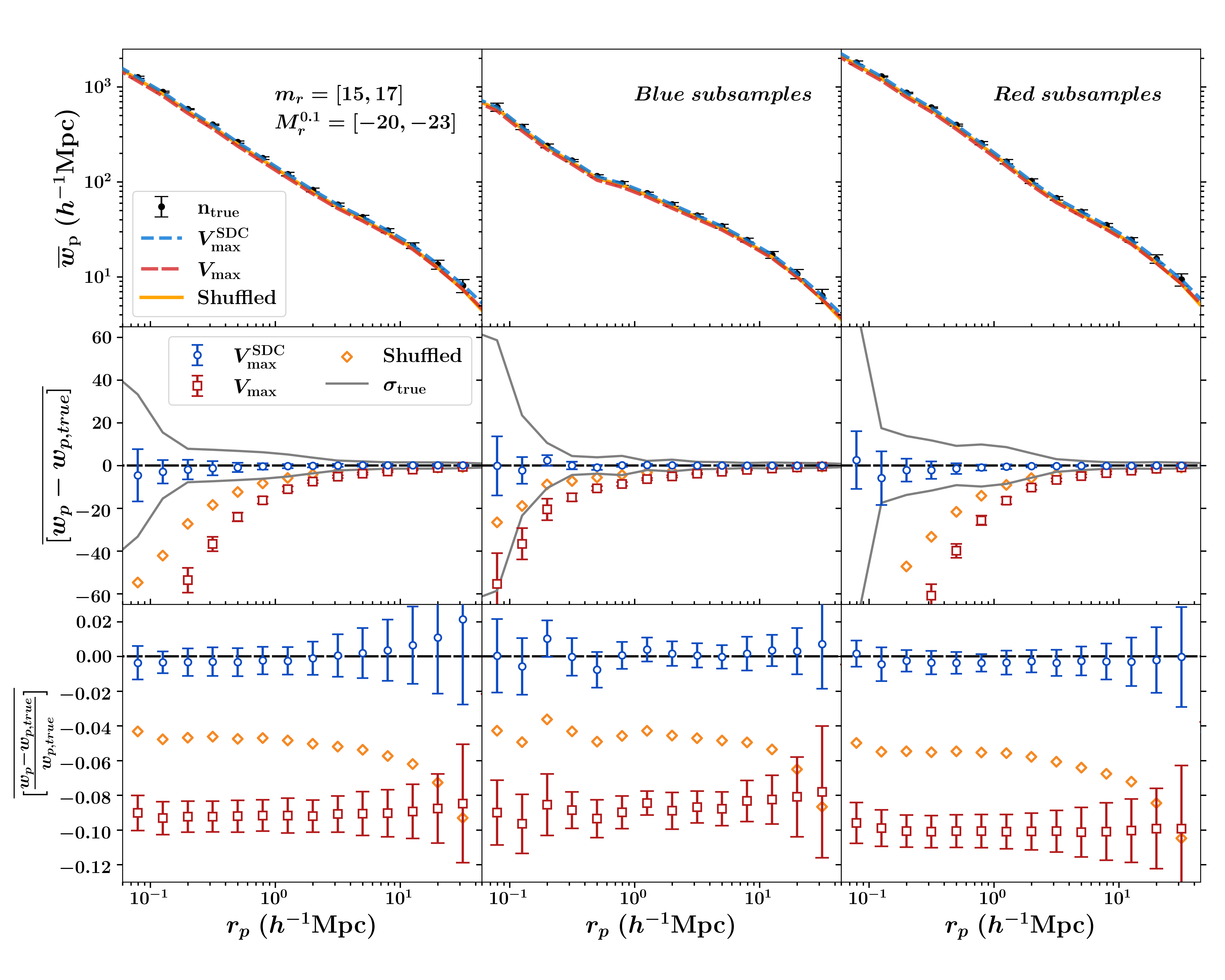
Figure 7: The same as Figure 6 but for the LS2 samples (left panels) and their blue (middle panels) and red (right panel) subsamples.

The projected 2PCFs for the LC samples without and with simple $k+e$ corrections are compared in Figure 4 and Figure 5, respectively. We compare the average projected 2PCF estimated using random catalogs produced by the radial selection models outlined in Section 4.1. In the left and right panels for the LC1 and LC2 samples, respectively, the estimated mean $\overline{w}_{p}$ of the 60 mock samples are displayed. In the top panels, $\overline{w}_{p,true}$ computed using the random catalog from the $n_{true}$ model is represented by solid black points with errors representing the $1\sigma$ dispersion across individual $w_{p,true}$s of samples. The blue-dashed, green-dotted, red long-dashed, and orange lines represent $\overline{w}_{p}$s estimated from random catalogs of the ${V^{\rm SDC}_{\rm max}}$, ${V^{\rm DC}_{\rm max}}$, ${V_{\rm max}}$, and shuffled methods, respectively. The average offsets $\overline{[w_{p}-w_{p,true}]}$ from $w_{p,true}$ for the models are shown in the middle row of panels, which are defined as $\overline{[w_{p}-w_{p,true}]}=\frac{1}{60}\sum^{60}_{i=1}{(w^{i}_{p}-w^{i}_{p,true})}$, where $w^{i}_{p}$ is the projected 2PCF measured for the $i$th LC sample. The offsets increase when the scale drops below $1{h^{-1}\rm Mpc}$ for both the ${V^{\rm DC}_{\rm max}}$ method (green-dotted lines) and the shuffled method (orange diamonds). When using the random catalogs of the ${V^{\rm SDC}_{\rm max}}$ technique to measure $w_{p}$, the little positive offsets in the blue open rolls with error bars indicate a slight overestimation on scale $r_{p}\lesssim 0.4{h^{-1}\rm Mpc}$. On a small scale, there are apparent offsets for the ${V_{\rm max}}$ approach for LC1 samples in both $k+e$ correction cases, as can be seen by the open red squares with error bars. For the LC2 samples, there are extremely modest systematic offsets for the ${V_{\rm max}}$ technique across all of the scales tested, and these offsets are smaller than those for the ${V^{\rm SDC}_{\rm max}}$ method. Compared to the $1\sigma_{true}$ (gray solid lines) among 60 $w_{p,true}$s, the ${V^{\rm SDC}_{\rm max}}$ and ${V_{\rm max}}$ methods’ offsets are essentially insignificant.

In the bottom panels of Figure 4 and Figure 5, we display the average deviation from $w_{p,true}$ for each model, using the same color-coded symbols and lines as the middle panels. The mean deviation $\overline{[(w_{p}-w_{p,true})/w_{p,true}]}$ is calculated from the 60 mock samples in the same manner as $\overline{[(w_{p}-w_{p,true})]}$. Clearly, the $w_{p}$ derived using random catalogs from the ${V^{\rm SDC}_{\rm max}}$ approach provide a mostly unbiased estimate of the genuine projected 2PCFs for both the LC1 and LC2 samples in both the no $k+e$ correction case (Figure 4) and the simple $k+e$ correction case (Figure 5). The $1\sigma$ deviations among the 60 samples for the ${V^{\rm SDC}_{\rm max}}$ approach (blue error bars) are significantly smaller than those for the ${V_{\rm max}}$ method (red error bars). For the LC1 samples in both $k+e$ correction cases, the ${V_{\rm max}}$ approach underestimates $w_{p}$ by less than 1%, and this bias worsens as the scale grows. At $r_{p}\sim 30{h^{-1}\rm Mpc}$, the bias reaches 13% with a substantial variance . For the LC2 samples, the measurement accuracies for both the ${V^{\rm SDC}_{\rm max}}$ and ${V_{\rm max}}$ methods are equivalent at scale $r_{p}\lesssim 4{h^{-1}\rm Mpc}$ for both methods. On a larger scale, the deviation of the ${V_{\rm max}}$ method grows to 4%, but remains within the margin of error. These discrepancies in $w_{p}$ from $w_{p,true}$ for the ${V_{\rm max}}$ model are mostly attributable to density fluctuations in galaxy samples. The $w_{p}$ measured using random catalogs from the ${V^{\rm DC}_{\rm max}}$ approach are overestimated at scale $r_{p}\lesssim 2{h^{-1}\rm Mpc}$ and underestimated at larger scales for both the LC1 and LC2 samples as shown in the bottom panels (green-dashed lines) of Figure 4 and Figure 5. As can be seen in Figure 1 and Figure 2, this tendency of deviation is the result of small fluctuations in the radial distribution of the random catalog generated by the ${V^{\rm DC}_{\rm max}}$ model. In essence, the fluctuations increase the number of RR pairs at the fluctuation scale, resulting in an underestimation of $w_{p}$. Due to the integral constraint effect, a small-scale overestimation of $w_{p}$ is unavoidable. After smoothing out the fluctuations, the ${V^{\rm SDC}_{\rm max}}$ approach yields estimates that are almost unbiased of $w_{p,true}$. The results of the shuffled technique are consistent with Paper I, which shows that an underestimation of $w_{p}$ grows as the scale increases.

Due to the severe deviations of $w_{p}$ for the ${V^{\rm DC}_{\rm max}}$ model in the tests using the LC samples, the following comparison for the LS samples will focus on testing for the ${V^{\rm SDC}_{\rm max}}$, ${V_{\rm max}}$, and shuffled methods. Figure 6 and Figure 7 display the results of the comparison for the LS samples with the two luminosity cuts, respectively. The left, middle, and right panels, respectively, present $w_{p}$ comparisons for luminosity-dependent samples and their blue and red subsamples. From 10 mock galaxy samples, the mean $\overline{w}_{p}$, $\overline{[w_{p}-w_{p,true}]}$, and $\overline{[(w_{p}-w_{p,true})/w_{p,true}]}$ are calculated (from the top to bottom panels). The $n_{true}$, ${V^{\rm SDC}_{\rm max}}$, ${V_{\rm max}}$, and shuffled methods all utilize the same color-coded lines and symbols as those used for figures showing the LC samples. For the LS1 samples in Figure 6, the ${V^{\rm SDC}_{\rm max}}$ model produces tiny $w_{p}$ offsets from $w_{p,true}$, which are consistent with the findings for the LC samples. Significant offsets are seen for the ${V_{\rm max}}$ and shuffled methods, notably for the LS1 samples and their blue subsamples, where the offsets are more than a $1\sigma$ dispersion of $w_{p,true}$ at $r_{p}\lesssim 3{h^{-1}\rm Mpc}$ scale. The average deviations displayed in the bottom panels clearly demonstrate the superiority of the ${V^{\rm SDC}_{\rm max}}$ approach over the ${V_{\rm max}}$ and shuffled method when measuring projected 2PCFs. $\sim 0.5\%$ deviations are detected for both LS1 samples and their color-dependent subsamples, which is essentially within the $1\sigma$ error margin. For the ${V_{\rm max}}$ approach, $\overline{[(w_{p}-w_{p,true})/w_{p,true}]}$s deviate by 6%, 5%, and 9% for the LS1 samples, blue subsamples, and red subsamples, respectively, which are considerably larger than $1\sigma$ errors. At $r_{p}\lesssim 10{h^{-1}\rm Mpc}$, the mean deviations for the shuffled approach are marginally better than those for the ${V_{\rm max}}$ method, but worsen as the scale increases, which is consistent with the test results for the LC samples.

Figure 7 presents a comparison of the $w_{p}$ for the LS2 samples. The offsets from $w_{p,true}$ for the ${V^{\rm SDC}_{\rm max}}$ technique are roughly comparable with the LS1 sample results. The $w_{p}$ measured using random catalogs from the ${V_{\rm max}}$ approach exhibit large offsets from $w_{p,true}$ that are worse than the offsets for the shuffled method on small scales, particularly for the LS2 samples (left middle panel) and red subsamples (right middle panel). In the bottom panels of Figure 7, the accuracy of measurement for three models is shown clearly. At scale $r_{p}<1{h^{-1}\rm Mpc}$, there is a $\sim 0.5\%$ underestimate for the LS2 samples (bottom left panel). At a larger scale, this deviation becomes an overestimation, reaching 2% at $r_{p}\sim 30{h^{-1}\rm Mpc}$ while being within the margin of error. The mean deviations for the blue and red subsamples are well constrained within 1%. The results of the ${V_{\rm max}}$ approach exhibit larger mean deviations than the LS1 samples, which are even worse than the results of the shuffled method. The deviations for the LS2 samples, blue subsamples, and red subsamples are roughly 9%, 8%, and 10%, respectively. The $w_{p}$ determined for the red subsamples exhibit more severe departures from $w_{p,true}$ for the ${V_{\rm max}}$ technique for both the LS1 and LS2 samples, demonstrating density fluctuations have a greater impact on clustering determination for red galaxies.

To better quantify the measurement accuracy of projected 2PCF for various radial selection models, we calculate the $\chi^{2}$ between $w_{p}$ and $w_{p,true}$ for the ${V^{\rm SDC}_{\rm max}}$, ${V_{\rm max}}$, and shuffled methods, respectively, as shown in Table 1. $\chi 2$ is computed as follows:

$$\chi^{2}=\sum^{N}_{i=0}\frac{(w^{i}_{p}-w_{p,true})^{2}}{\sigma^{2}_{true}}.$$ (11)

The number of mock samples $N$ is 60 for LC samples and 10 for the LS samples. For the LC samples, with the exception of the LC2 samples with simple $k+e$ corrections for which $\chi^{2}$ of the ${V^{\rm SDC}_{\rm max}}$ and ${V_{\rm max}}$ methods are essentially equal, the $w_{p}$ of the ${V^{\rm SDC}_{\rm max}}$ method exhibit the least $\chi^{2}$ from $w_{p,true}$ when compared to the other two models. For all LS samples and their blue and red subsamples, the ${V^{\rm SDC}_{\rm max}}$ approach also yields the least $\chi^{2}$ among the three methods. The $\chi^{2}$ values for the LS samples are greater than those for the LC samples for all three models. This may probably be due to the fact that the LS samples built from a light cone catalog contain more complicated $k+e$ corrections than LC samples. On the basis of the preceding figures and $\chi^{2}$ tests, we demonstrate that the $w_{p}$ measured using the random catalogs generated by the ${V^{\rm SDC}_{\rm max}}$ approach result in the least deviation from $w_{p,true}$ for both flux-limited samples and their color-dependent subsamples. In Section 5, we discuss the performance of the radial selection models for the LC and LS samples.

Table 1: $\chi^{2}$ of the Projected 2PCFs for the Mock Samples

Samples		$\chi^{2}$
	${V^{\rm SDC}_{\rm max}}$	${V_{\rm max}}$	Shuffled
LC1($no~{}k+e$)	1.364	6.264	107.225
LC2($no~{}k+e$)	1.460	4.254	62.329
LC1($simple~{}k+e$)	3.531	6.351	108.770
LC2($simple~{}k+e$)	2.757	2.667	106.466
LS1	1.893	1618.495	977.362
LS1 (blue)	33.013	161.187	124.543
LS1 (red)	19.525	2769.991	1988.678
LS2	45.168	3416.047	857.843
LS2 (blue)	63.572	925.400	240.416
LS2 (red)	71.431	5054.464	1562.508

4.2.3 Comparison of the Redshift-space 2PCFs

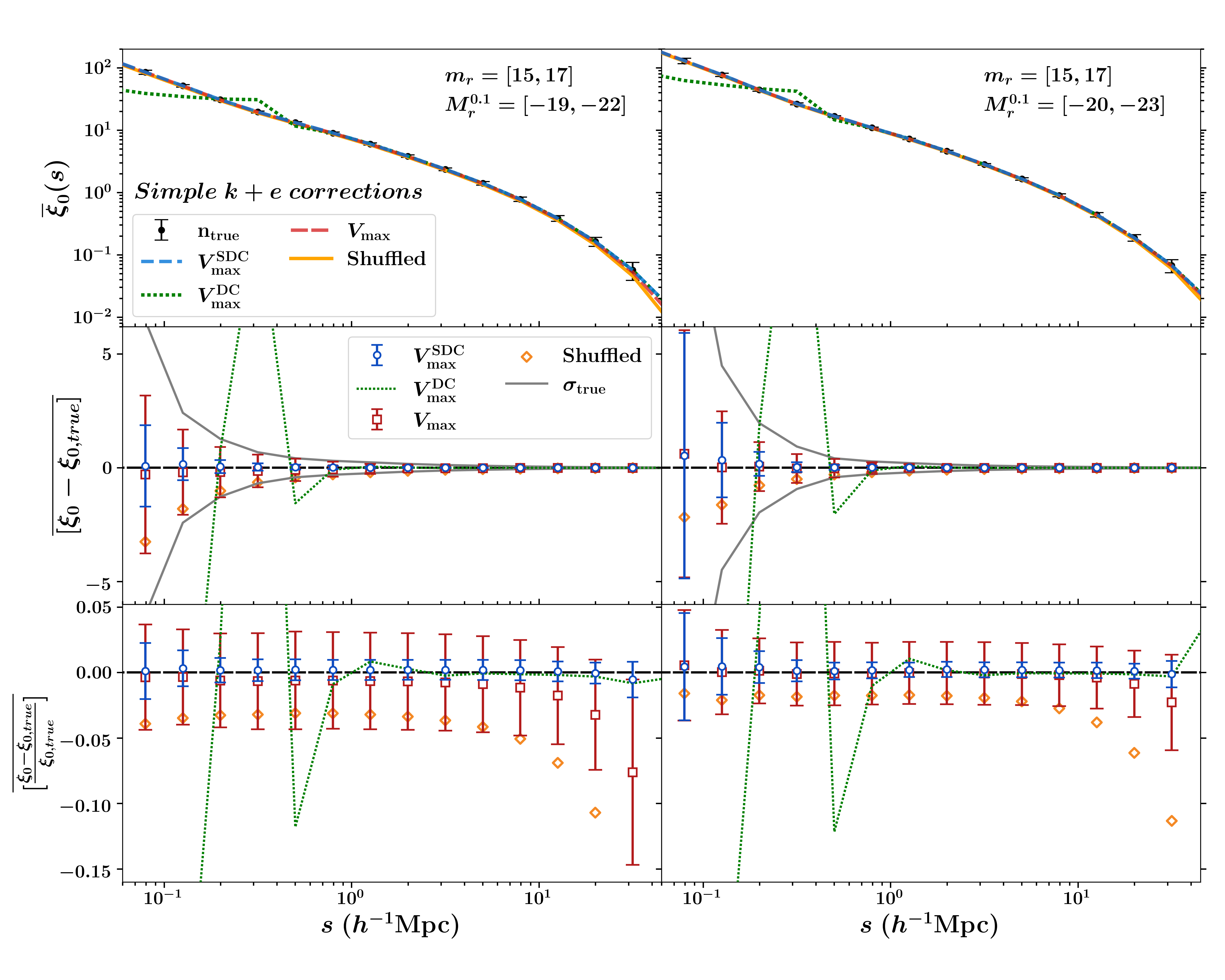
Figure 8: Similar to Figure 4, with a comparison of the $\xi_{0}$ for the redshift-space 2PCFs of the LC1 samples (left panels) and LC2 samples (right panels) with simple $k+e$ corrections.

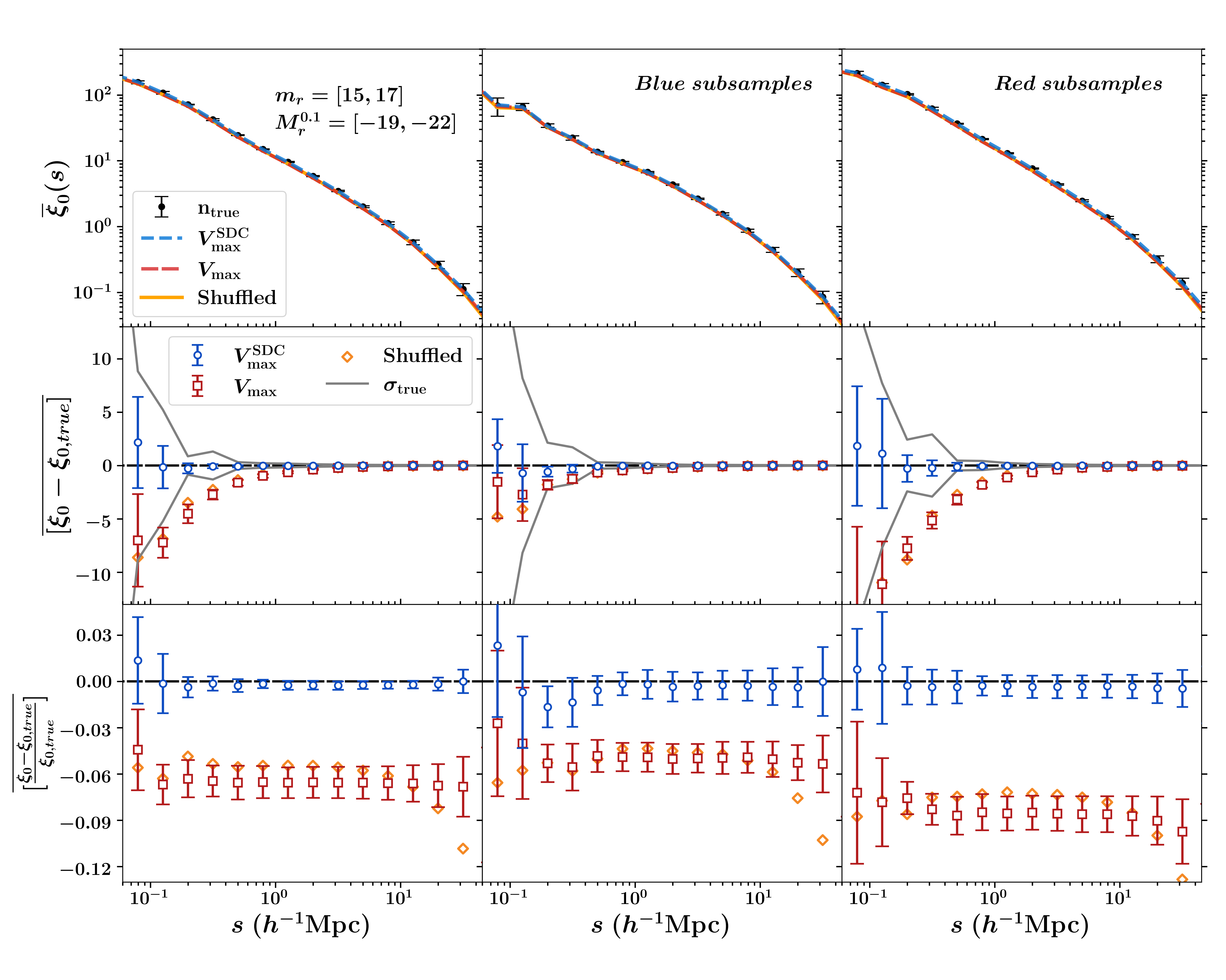
Figure 9: Similar to Figure 6, with a comparison of the $\xi_{0}$ for the redshift-space 2PCFs of the LS1 samples (left panels) and their blue (middle panels) and red (right panels) subsamples.

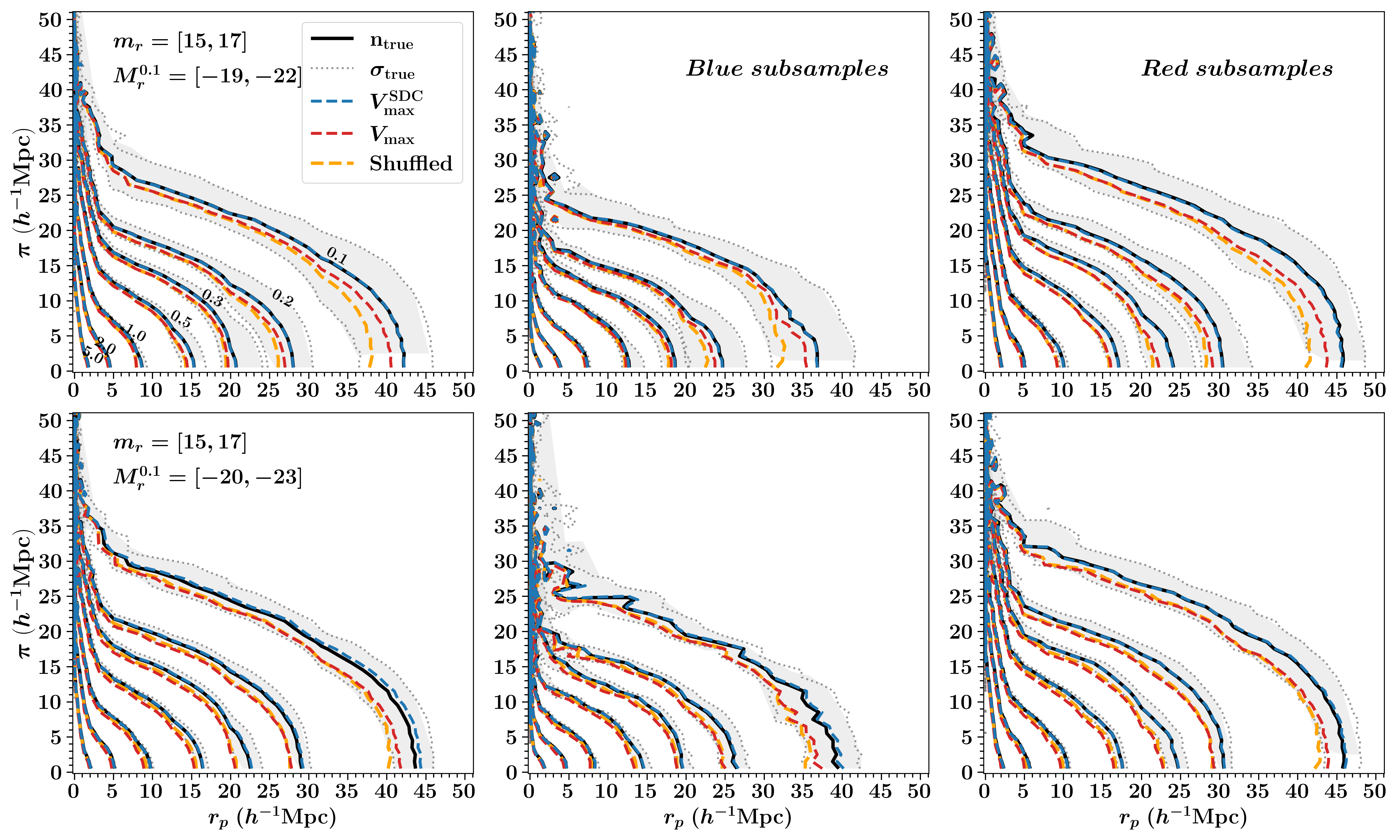
Figure 10: Comparison of the average 2D correlation function $\overline{\xi}(r_{p},\pi)$ for the luminosity-dependent flux-limited samples. The L1-C1, L2-C1, and L3-C1 samples are shown from top to bottom accordingly, their blue/red subsamples are shown in the middle and right panels in each row. Here, $\overline{\xi}(r_{p},\pi)$ is the averaged $\xi(r_{p},\pi)$ among the 60 mock samples. The true $\overline{\xi}(r_{p},\pi)$ measured using the random catalog from the $n(z)_{\rm true}$ method is shown as the black contour. The gray-shaded region with dotted lines marks the $1\sigma$ scatter of the true $\overline{\xi}(r_{p},\pi)$ among the 60 mock samples. The yellow, red, and blue-dashed contours denote the $\overline{\xi}(r_{p},\pi)$ of the shuffled, ${V_{\rm max}}$, and ${V^{\rm SDC}_{\rm max}}$ methods, respectively. The contour levels from outside-in correspond to $\overline{\xi}(r_{p},\pi)=[0.1,0.2,0.3,0.5,1.0,2.0,5.0]$. The middle and right column panels show s comparison of the blue/red subsamples

The redshift-space correlation functions are compared in the same manner as $w_{p}$ for both the LC and LS samples, and the results for different radial selection models are generally consistent with the comparisons for $w_{p}$ in the previous section. The mean $\overline{\xi}_{0}$, $\overline{[\xi_{0}-\xi_{0,true}]}$, and $\overline{[(\xi_{0}-\xi_{0,true})/\xi_{0,true}]}$ for the LC samples with simple $k+e$ corrections are shown in Figure 8, from top to bottom, respectively. Estimates of $\xi_{0}$ derived from the random catalogs created by the ${V^{\rm SDC}_{\rm max}}$ approach display the smallest offsets and deviations from $\xi_{0,true}$ for both the LC1 (left panels) and LC2 (right panels) samples. For the ${V^{\rm DC}_{\rm max}}$ technique, the $\xi_{0}$ at scale $r_{p}<1{h^{-1}\rm Mpc}$ exhibit large offsets and deviations compared to the findings of $w_{p}$. For the ${V_{\rm max}}$ method, $\xi_{0}$ deviations are marginally attenuated compared to the results of $w_{p}$, indicating that the impact of density fluctuations on clustering is less significant in redshift space. The $\xi_{0}$ for the shuffled approach exhibit the same offsets and deviations from $\xi_{0,true}$ as $w_{p}$. As the results of the LC samples without $k+e$ corrections are similar to those shown in Figure 8, they are omitted here.

Figure 9 illustrates the comparison of $\xi_{0}$ for the LS1 samples (left panels), and their blue (middle panels) and red (right panels) subsamples, respectively. Compared to the ${V_{\rm max}}$ and shuffled methods, the ${V^{\rm SDC}_{\rm max}}$ approach produces the least offsets and deviations from $\xi_{0,true}$ for the LS1 samples and red subsamples. For the blue subsamples, the ${V^{\rm SDC}_{\rm max}}$ method’s mean offset at $s\sim 0.07{h^{-1}\rm Mpc}$ is slightly larger than the ${V_{\rm max}}$ method’s mean offset, and both approaches have comparable deviations at that scale. This is not a concern because the amount of uncertainty at this scale is also high due to the shot noise. In general, on $\xi_{0}$ measurements, the ${V^{\rm SDC}_{\rm max}}$ technique continues to outperform the other two radial selection models. Since the findings of the LS2 samples are basically consistent with Figure 9, they are also excluded here.

In Figure 10, the average 2D correlation functions $\overline{\xi}(r_{p},\pi)$ for the LS samples are presented. The $\overline{\xi}(r_{p},\pi)$ for the LS1 samples (left panel), blue subsamples (middle panel), and red subsamples (right panel) are displayed in the upper panels. $\overline{\xi}(r_{p},\pi)$s for the $n_{true}$, ${V^{\rm SDC}_{\rm max}}$, ${V_{\rm max}}$, and shuffled methods are represented by black solid lines, blue-dashed lines, red-dashed lines, and yellow-dashed lines, respectively. The $1\sigma_{true}$ dispersion of $\xi_{true}(r_{p},\pi)$ among the 10 mock samples is denoted by gray-dotted lines in places with shading. The $\overline{\xi}(r_{p},\pi)$ of the ${V^{\rm SDC}_{\rm max}}$ model provide the best agreement with $\overline{\xi}_{true}(r_{p},\pi)$ for the LS1 samples and color-dependent subsamples. For $\overline{\xi}(r_{p},\pi)$ of the ${V_{\rm max}}$ and shuffled methods, there are offsets of varying degrees; yet, the offsets stay within the $1\sigma_{true}$ error margins; however, the contour shapes are altered. In the lower panels displaying $\overline{\xi}(r_{p},\pi)$s for the LS2 samples, the majority of contours for the ${V^{\rm SDC}_{\rm max}}$ model are consistent with $\overline{\xi}_{true}(r_{p},\pi)$. $1\%\sim 2\%$ deviations are seen in $\overline{w}_{p}$ (bottom left panel in Figure 7) for both LS2 samples and blue subsamples are also observed in contours at large scale. For the ${V_{\rm max}}$ and shuffled methods, the offsets in the $\overline{\xi}(r_{p},\pi)$ contours are close to the error margins of $1\sigma_{true}$; thus, the contour shapes are altered as well. Since the comparisons for the LC samples are substantially identical to those in Figure 10, they are excluded here.

5 Discussion

Our tests demonstrate that for flux-limited sample with a redshift-dependent number density $n(z)$, utilizing the random catalog generated by the ${V^{\rm SDC}_{\rm max}}$ technique to measure galaxy clustering produces the least deviation from the true clustering when compared to the other radial selection methods. Some aspects of the performance of the ${V^{\rm SDC}_{\rm max}}$ technique remain to be clarified and discussed, as detailed below.

5.1 Impact of Smoothness Parameters on Clustering Estimation

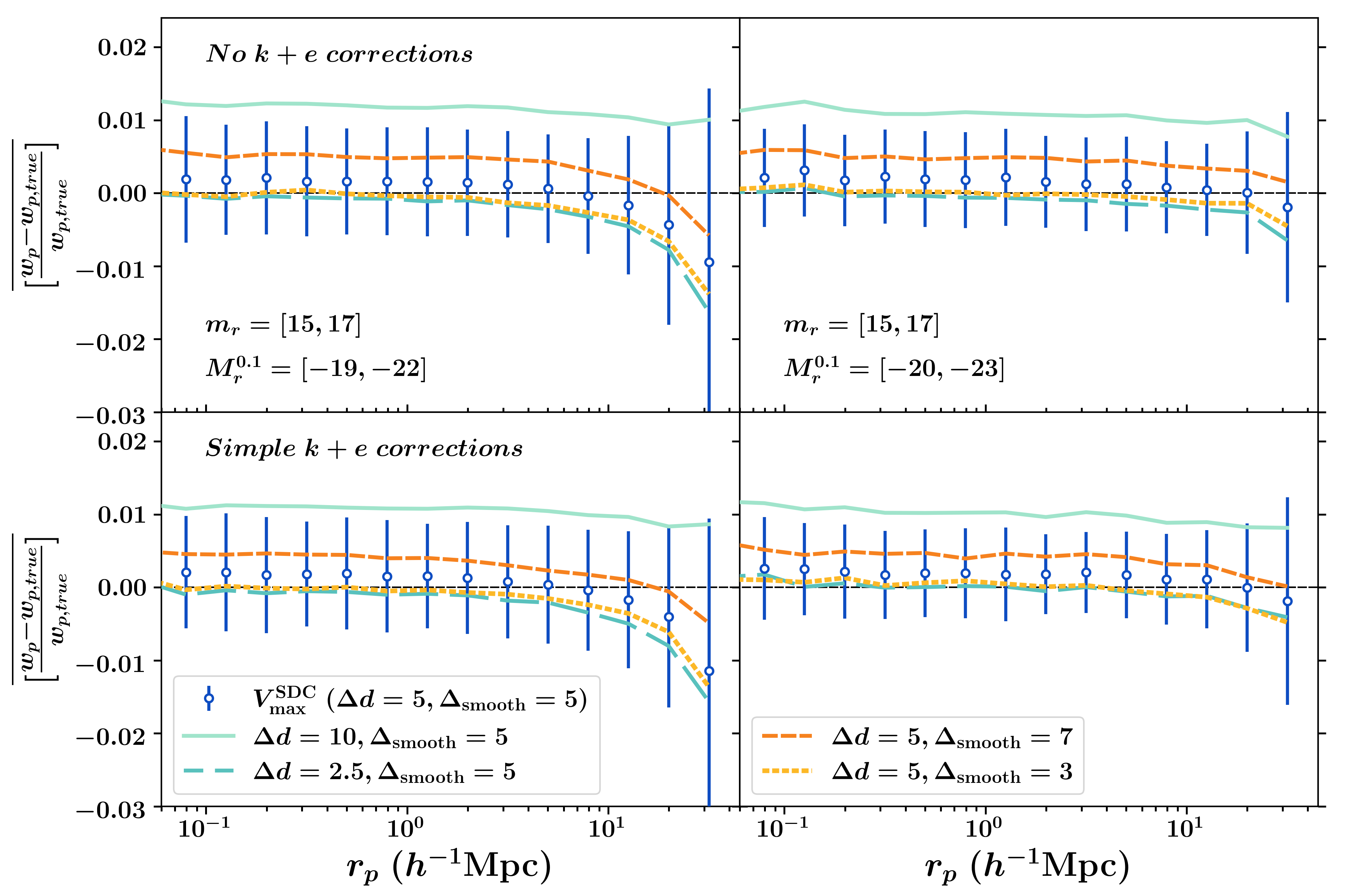
Figure 11: The average deviations of $w_{p}$ from $w_{p,true}$ for the ${V^{\rm SDC}_{\rm max}}$ method, in which alternative histogram bin sizes and smooth box sizes are adopted in the smooth process in order to assess the impact of multiple choices on clustering estimation. The fiducial bin size and smooth box size used in Section 4.2 are $\Delta d=5{h^{-1}\rm Mpc}$ and $\Delta_{\rm smooth}=5$, respectively, as indicated by the open blue circles with error bars. The alternate histogram bin sizes are $\Delta d=2.5{h^{-1}\rm Mpc}$ and $\Delta d=10{h^{-1}\rm Mpc}$, with the same smooth box size as the fiducial one, as indicated by the green-dashed lines and the light blue lines, respectively. The alternate smooth box sizes are $\Delta_{\rm smooth}=$ 3 and 7, with the same fixed histogram bin size as the fiducial one, as shown by the yellow short-dashed and orange long-dashed lines, respectively. The zero deviation is shown by the horizontal black-dashed lines. Upper panels: tests for the LC1 samples (left panel) and LC2 samples (right panel) for the no $k+e$ correction case. Lower panels: similar tests for LC1 and LC2 samples to those in the upper panels, but for the simple $k+e$ correction case.

For the ${V^{\rm SDC}_{\rm max}}$ approach, we add a smoothing step to eliminate the unanticipated small fluctuations in the redshift distribution of the cloned random galaxies generated by the ${V^{\rm DC}_{\rm max}}$ method. The previous comparison of 2PCFs for the ${V^{\rm SDC}_{\rm max}}$ and ${V^{\rm DC}_{\rm max}}$ methods demonstrate the necessity of a smoothing procedure for a random catalog in order to produce a nearly unbiased clustering measurement for the flux-limited sample. Smoothing requires a selection of histogram bin size $\Delta d$ and smooth box size $\Delta_{\rm smooth}$. To determine the effect of varying $\Delta d$ and $\Delta_{\rm smooth}$ values on the final galaxy clustering determination, we vary these two smoothness parameters and regenerate random catalogs to perform the estimate. First, we set $\Delta d=5{h^{-1}\rm Mpc}$ and $\Delta_{\rm smooth}=5$ as the fiducial case, which we have used for the ${V^{\rm SDC}_{\rm max}}$ technique in the previous tests in Section 4.2. Second, we chose $\Delta d=2.5{h^{-1}\rm Mpc}$ and $10{h^{-1}\rm Mpc}$ for the histogram bin size, with $\Delta_{\rm smooth}=5$ set to smooth. Thirdly, we select $\Delta_{\rm smooth}=3$ and $7$ for the smoothing with $\Delta d=5{h^{-1}\rm Mpc}$ set. Figure 11 displays the average deviations of $w_{p}$ from $w_{p,true}$ for the random catalogs created by the ${V^{\rm SDC}_{\rm max}}$ technique with various $\Delta d$ and $\Delta_{\rm smooth}$ values. To simplify the assessment, we just test the projected 2PCFs of the LC samples here. In the absence of $k+e$ corrections, the upper panels of Figure 11 depict the mean deviations of $w_{p}$ for the LC1 (left panel) and LC2 (right panel) samples, respectively. We can see that a finer value of $\Delta d=2.5{h^{-1}\rm Mpc}$ (green-dashed lines) and $\Delta_{\rm smooth}=3$ (light blue lines) lead to a constant drop in $\overline{[(w_{p}-w_{p,true})/w_{p,true}]}$ on all test scales, resulting in reduced deviations at $r_{p}\lesssim 2{h^{-1}\rm Mpc}$ and an underestimate on a larger scale, especially for the LC1 samples. In contrast, a coarser size of $\Delta_{\rm smooth}=7$ (orange long-dashed lines) results in an overall increase relative to the mean deviation in the fiducial case (open blue rolls with error bars), resulting in an overestimation at scale $r_{p}\lesssim 20{h^{-1}\rm Mpc}$. A coarser size of $\Delta d=10{h^{-1}\rm Mpc}$ (yellow short-dashed lines) leads to an $\sim 1\%$ increase in the mean deviation of $w_{p}$ relative to the deviation in the fiducial case; this is the only mean deviation that exceeds the $1\sigma$ errors but is still around $\sim 1\%$. In the lower panels, the test results for the LC samples with simple $k+e$ corrections are displayed, which are essentially identical to the findings in the above panels, suggesting that the smooth process is insensitive to galaxy samples when different $k+e$ corrections are applied. Our tests indicate that the variation in $\Delta d$ and $\Delta_{\rm smooth}$ in the smooth process of the ${V^{\rm SDC}_{\rm max}}$ technique affects the accuracy of clustering measurement; however, the effect of deviations is much less than 1%. The advantage of the ${V^{\rm SDC}_{\rm max}}$ technique over the other radial selection models still stands.

5.2 Difference in Clustering Uncertainty

In prior tests, the uncertainties in clustering deviations among the 60 LC samples are significantly larger than the uncertainties in the 10 LS samples, which is not expected intuitively. In addition, the deviation uncertainties for the ${V^{\rm SDC}_{\rm max}}$ approach are approximately a fourth of those for the ${V_{\rm max}}$ method in the LC samples. As can be seen in Figure 12, we further investigate the radial distribution of the LC and LS samples in order to determine the probable distinct drivers of these discrepancies. Here, we take into account the LC samples without $k+e$ corrections and the LS1 samples, which are sufficient to explain the difference in uncertainty. First, we compute the normalized radial distribution for the galaxy samples and random catalogs created using the $n(z)_{\rm true}$, ${V^{\rm SDC}_{\rm max}}$, and ${V_{\rm max}}$ methods, respectively. To quantify the density fluctuations relative to the true smooth distribution created by the $n(z)_{\rm true}$ method, we estimate the average deviations $\overline{\Delta}$ and $1\sigma$ variances of these distributions from the genuine normalized distribution for the 60 LC samples and 10 LS1 samples separately, as shown in Figure 12 from top to bottom.

The $\overline{\Delta}$ and $1\sigma$ variance for the galaxy samples are shown by the thick gray and thin light gray lines. For both the LC1 (upper panel) and LC2 (middle panel) samples, the variations across the 60 individual samples vary greatly, as indicated by $1\sigma$ variance, whereas $\overline{\Delta}$ exhibits a relatively small deviation from the true normalized distribution. The light yellow and light orange regions denote the locations in which 90% and 60% of the expected random galaxies are likely to be distributed, and we anticipate that the bulk of pairs used to estimate clustering are from 90% region. $\overline{\Delta}$ (red thick lines) and $\sigma$ (light red thin lines) of the ${V_{\rm max}}$ technique reveal that this approach corrects the fluctuations in the galaxy samples; nonetheless, the imprints of large-scale structures are still discernible. For instance, $\overline{\Delta}$ for the LC1 samples shows a small but observable deviation at $100\sim 450{h^{-1}\rm Mpc}$ where 90% of galaxies are located. This explains the consistent bias noticed in $w_{p}$ and $\xi$ in previous testing. For the LC2 samples, the systematic bias is almost imperceptible, with just a tiny overestimation at $d\gtrsim 500{h^{-1}\rm Mpc}$, indicating a clustering bias that has been detected in prior tests. For the ${V^{\rm SDC}_{\rm max}}$ approach, there are noisy fluctuations in $\overline{\Delta}$ (blue thick lines) for both the LC1 and LC2 samples, indicating that the smoothing does not eliminate all noisy fluctuations in the radial distribution and there is still room to improve the smoothing. Fortunately, these fluctuations are complimentary to a certain degree, yielding a substantially unbiased measurement for galaxy clustering. We observe that the $1\sigma$ errors (light blue thin lines) for the ${V^{\rm SDC}_{\rm max}}$ approach are less than those for the ${V_{\rm max}}$ method, especially for the LC1 samples at the 60% region. This is essentially the reason for the substantial difference in uncertainty found between the two techniques for $w_{p}$ and $\xi$, demonstrating once again that the ${V^{\rm SDC}_{\rm max}}$ method can more successfully rectify the effect of density fluctuations on individual samples, and thus the clustering estimations converge to the genuine galaxy clustering.

As demonstrated in the bottom panel, $\overline{\Delta}$ for the LS1 samples deviates significantly from the genuine distribution when compared to the LC samples. By rotating the sky, just 10 LS1 samples are created from a single light cone catalog. These samples have a significantly reduced $1\sigma$ variance than LC samples, particularly at the $60\%$ region. In the LS1 samples, the advantage of density correction in the ${V^{\rm SDC}_{\rm max}}$ approach is exhibited more clearly compared to the ${V_{\rm max}}$ method. Both approaches have equal errors, but the $\overline{\Delta}$ of the ${V^{\rm SDC}_{\rm max}}$ method deviates less from the true distribution, resulting in a more accurate clustering measurement. In contrast, the ${V_{\rm max}}$ technique predicts too many random galaxies at $d\lesssim 400$ and fewer galaxies at high $d$ due to strong fluctuations in galaxy samples, hence exhibiting a greater deviation in $\overline{\Delta}$ in comparison to $\overline{\Delta}$ of the LC samples. This also explains the extremely systematic bias in $w_{p}$ observed for the ${V_{\rm max}}$ approach on all testing scales in earlier tests.

Last but not least, the LC samples and LS samples are derived from distinct parent mock catalogs utilizing two simulations with different resolutions and galaxy-halo connection models. Both the LC and LS samples are complete at $M^{0.1}_{\rm r}\leq-18$; however, the simulation of (Jing, 2019) used to generate the LC samples has a mass resolution that is an order of magnitude higher than that of the MXXL simulation (Angulo et al., 2012), implying that more halo and galaxy structures are resolved in the LC samples. Moreover, despite the fact that the LC samples are constructed using a simple galaxy-halo connection model with simple $k+e$ corrections, the benefit is that all model parameters are clear and straightforward; hence, the potential deviation and error sources are comprehendible. For the LS samples, with a more sophisticated galaxy evolution and $k$ correction, the light cone catalog of Smith et al. (2017) is theoretically closer to actual observation data; the main drawback is a restricted number of samples. The test results of these two sample groups demonstrate that either the $k+e$ corrections are based on simple or more complex and realistic mock catalogs, the ${V_{\rm max}}$ technique may produce an inaccurate measurement of galaxy clustering, whereas the ${V^{\rm SDC}_{\rm max}}$ method can always produce an accurate and precise estimate of clustering.

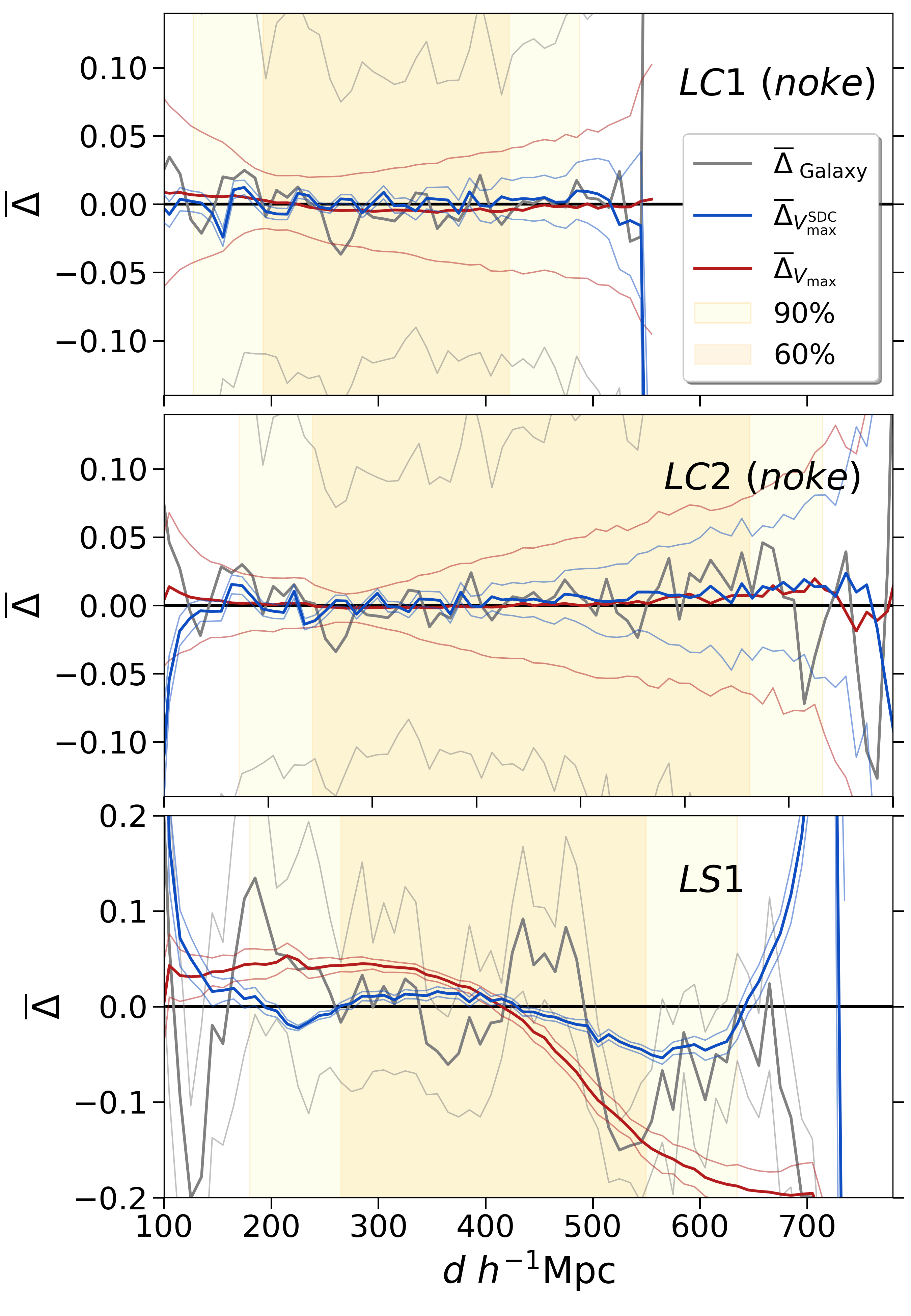
Figure 12: Top panel: the average deviations $\overline{\Delta}$ and $1\sigma$ errors from the radial distribution of the random catalog obtained by the $n(z)_{\rm true}$ method. The mean deviation is computed using the equation $\overline{\Delta}=\overline{(n^{i}-n^{i}_{true})/n^{i}_{true}}$, where $n^{i}$ is the normalized radial distribution of the $i$th LC1 sample and random catalog produced using the ${V^{\rm SDC}_{\rm max}}$ and ${V_{\rm max}}$ methods. The $\overline{\Delta}$ of the LC1 samples is shown by the thick gray lines, while the $1\sigma$ errors over the 60 samples are represented by the thin gray lines. The thick blue lines and thin light blue lines represent $\overline{\Delta}$ and errors for the random catalogs generated by the ${V^{\rm SDC}_{\rm max}}$ technique. The thick red lines and thin light red lines represent the ${V_{\rm max}}$ algorithm. The light yellow and light orange regions indicate the locations of 90% and 60% of galaxies, respectively. Middle panel: Similar to the top panel, it presents the average deviations and errors for the LC2 samples and their corresponding random catalogs. Bottom panel: Similar to top panel, it displays the average deviations and errors for the LS1 samples and their corresponding random catalogs.

6 Conclusions

In this paper, we provide a radial selection model, the ${V^{\rm SDC}_{\rm max}}$ approach, for generating the redshifts of random catalogs in galaxy two-point statistics that allows for a high level of accuracy and precision in the estimation. This method is an improvement on the density-corrected ${V_{\rm max}}$ method proposed by Cole (2011), and it consists mostly of three modifications: (1) adding an estimate of $z_{\rm min}$ and expanding the code’s application to a general flux-limited sample; (2) support for a redshift and color-dependent $k-$correction model applicable to individual galaxies; (3) adding a smooth step to the output cloned radial distribution of random galaxies. These modifications are crucial for obtaining a smooth radial distribution for a random catalog that is unaffected by galaxy density fluctuations, which is the key to a clustering measure with high precision and accuracy.

We measure 2PCFs using two groups of flux-limited samples, designated LC and LS, to validate the ${V^{\rm SDC}_{\rm max}}$ approach. The flux-limited LC samples are constructed from 10 mock catalogs with two luminosity cuts and two simple $k+e$ correction cases. Using the same sample selection criteria and luminosity thresholds as for the LC samples, t10 LS samples are generated using the light cone catalog of Smith et al. (2017). To test property-dependent clustering, the LS samples are subdivided into blue and red subsamples. We compare the projected and redshift-space 2PCFs using random catalogs created from the $n_{true}$, ${V^{\rm SDC}_{\rm max}}$, ${V^{\rm DC}_{\rm max}}$, ${V_{\rm max}}$, and redshift shuffled methods. Our test results demonstrate that the ${V^{\rm SDC}_{\rm max}}$ approach is the only reliable radial selection model capable of achieving sub-percent accuracy for $w_{p}$ measurement on scales ranging from $0.07{h^{-1}\rm Mpc}$ to $\sim 40{h^{-1}\rm Mpc}$. A $2\%$ deviation arises on a large scale for the LS2 sample; however, it is still less than the deviations of other radial selection models. In general, the ${V^{\rm SDC}_{\rm max}}$ technique can constrain the measurement accuracy of $w_{p}$ to within $1\%$ for color-dependent galaxy clustering, validating its superiority over the ${V_{\rm max}}$ and redshift shuffled methods.

The next generation of spectroscopic surveys, specifically the DESI experiment, will obtain the spectra of around 40 million galaxies and quasars over 14,000 $deg^{2}$, which is almost an order of magnitude more than the previously observed galaxies (Myers et al., 2022). These extragalactic objects include 13 million bright galaxy sample (a magnitude of 2 deeper than the SDSS main sample) (Lan et al., 2023), 8 million luminous red galaxies, 16 million emission line galaxies, and 3 million quasars (Levi et al., 2013; DESI Collaboration et al., 2016a, b; Raichoor et al., 2022). On the one hand, the two-point statistics of these up-coming galaxies will surely afford us an unprecedented opportunity to comprehend the physics of galaxy formation and evolution, improve the galaxy-halo connection, and shed light on the role of the halo environment in determining the galaxy’s physical properties (Ferreira et al., 2022). On the other hand, how to fully exploit these galaxies, particularly with the assistance of the galaxy 2PCFs, remains a challenge. Using volume-limited catalogs to conduct the 2PCF analysis will not only result in the rejection of a considerable number of galaxies, but it may also lead to the loss of crucial information imprinted in clustering. The density-corrected ${V_{\rm max}}$ approach proposed by (Cole, 2011) solves this problem, and our improvements and tests confirm that the ${V^{\rm SDC}_{\rm max}}$ method is a viable technique for accurately measuring clustering for flux-limited and color-dependent samples, hence maximizing the use of galaxies. Our present tests are preliminary, concentrating mostly on low-redshift galaxies. In the future, we will continue to improve this approach and conduct more tests on various properties of galaxies (e.g., stellar mass, star-formation rate, and so forth) as well as tests employing relative high-redshift galaxies (e.g., CMASS, BOSS and eBOSS) and mocks.

Appendix A Mock Samples

As an example, Figure 13 displays the estimated average galaxy number density $\overline{n}(z)$ for the 60 LC samples. The $\overline{n}(z)$ of these flux-limited samples changes as a function of comoving distance. The $\overline{n}(z)$s of the LC samples are in excellent agreement with the predicted input $n_{\rm DR7}$ derived from the input LF and the corresponding sample selection criteria. As predicted, $\overline{n}(z)$ for the LS2 samples contains more brighter and high-redshift galaxies than $\overline{n}(z)$ for the LS1 samples. In addition, the $\overline{n}(z)$ for the samples with simple $k+e$ corrections exhibits a slight evolution toward higher redshift when compared to samples without $k+e$ corrections.

Figure 14 displays the LS samples on the redshift-magnitude diagram (left panel) and color-magnitude diagram (right panel), respectively. The flux-limited LS samples are constructed from a light cone catalog with two luminosity cuts. At the low-redshift regions, the light cone catalog mimics the SDSS DR7 data and hence, has an LF of Blanton et al. (2003). We use the method described in Zehavi et al. (2011) to divide the galaxies into blue and red galaxies, as indicated by the red line in the right panel. Additionally, the LS samples have a redshift-dependent number density identical to that observed in Figure 13 and spanning a broader redshift range.

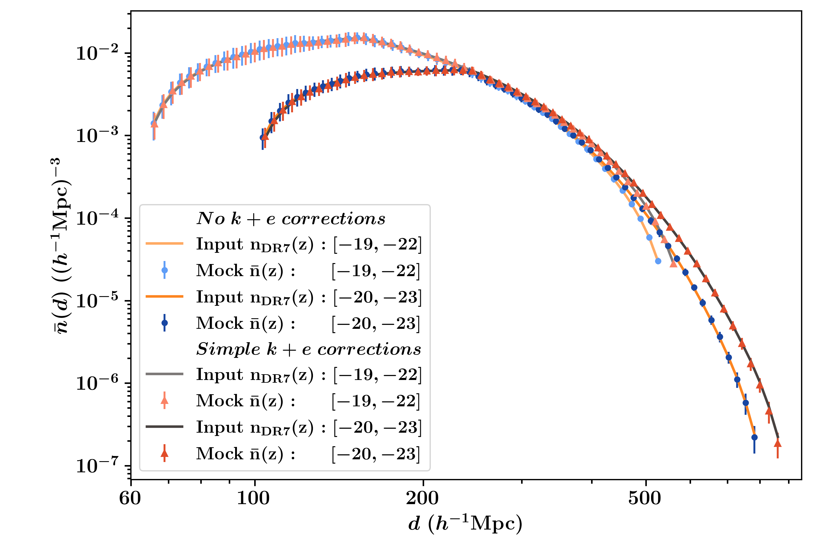
Figure 13: The mean number density $\overline{n}(z)$ among the 60 LC mock samples. These samples have a flux cut at $m_{r}=[15,17]$ and two luminosity cuts at $M^{0.1}_{r}=[-19,-22]$ for the LC1 samples and $M^{0.1}_{r}=[-20,-23]$ for the LC2 samples. In the case of no $k+e$ corrections, the light blue and dark blue points with error bars represent the $\overline{n}(z)$ and $1\sigma$ variance for the LC1 and LC2 samples, respectively. The orange and light orange lines show the input $n_{\rm DR7}$ derived by the input LF and sample selection criteria. In the case of simple $k+e$ corrections, the orange and red triangles with errors indicate $\overline{n}(z)$ and $1\sigma$ for the LC1 and LC2 samples, respectively. The inputs $n_{\rm DR7}$ are shown in gray and light gray lines.

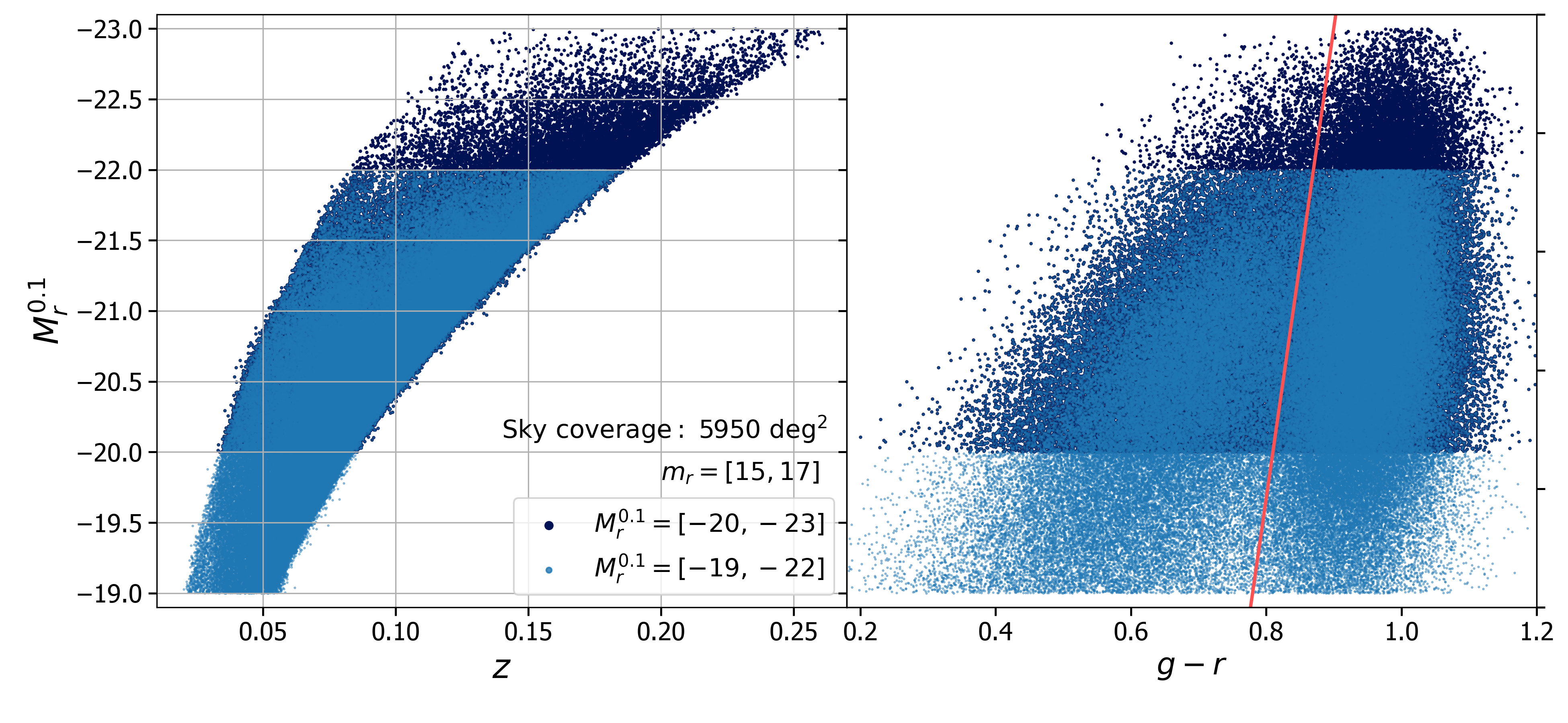
Figure 14: Left panel: the LS samples on the magnitude-redshift diagram. The light blue points denote galaxies in one of the LS1 samples with a flux cut at $m_{r}=[15,17]$ and luminosity cut at $M^{0.1}_{\rm r}=[-19,-22]$. The dark blue points stand for one of the LS2 samples with cuts of $m_{r}=[15,17]$ and $M^{0.1}_{\rm r}=[-20,-23]$. The samples have a sky coverage of $5950\deg^{2}$. Right panel: the LS samples on the color-magnitude diagram. The LS1 and LS2 samples are color coded similarly to those in the panel on the left. The red line as referred to by Zehavi et al. (2011) splits galaxies into blue and red subsamples.

References

- Alam et al. (2021a) Alam, S., de Mattia, A., Tamone, A., et al. 2021a, MNRAS, 504, 4667, doi: 10.1093/mnras/stab1150
- Alam et al. (2021b) Alam, S., Aubert, M., Avila, S., et al. 2021b, Phys. Rev. D, 103, 083533, doi: 10.1103/PhysRevD.103.083533
- Amendola et al. (2013) Amendola, L., Appleby, S., Bacon, D., et al. 2013, Living Reviews in Relativity, 16, 6, doi: 10.12942/lrr-2013-6
- Amin et al. (2022) Amin, M. A., Cyr-Racine, F.-Y., Eifler, T., et al. 2022, arXiv e-prints, arXiv:2203.07946. https://arxiv.org/abs/2203.07946
- Angulo et al. (2012) Angulo, R. E., Springel, V., White, S. D. M., et al. 2012, MNRAS, 426, 2046, doi: 10.1111/j.1365-2966.2012.21830.x
- Behroozi et al. (2019) Behroozi, P., Wechsler, R. H., Hearin, A. P., & Conroy, C. 2019, MNRAS, 488, 3143, doi: 10.1093/mnras/stz1182
- Bennett et al. (2013) Bennett, C. L., Larson, D., Weiland, J. L., et al. 2013, ApJS, 208, 20, doi: 10.1088/0067-0049/208/2/20
- Berlind et al. (2006) Berlind, A. A., et al. 2006, ApJS, 167, 1, doi: 10.1086/508170
- Beutler et al. (2014) Beutler, F., Saito, S., Seo, H.-J., et al. 2014, MNRAS, 443, 1065, doi: 10.1093/mnras/stu1051
- Bianchi & Percival (2017) Bianchi, D., & Percival, W. J. 2017, MNRAS, 472, 1106, doi: 10.1093/mnras/stx2053
- Bianchi & Verde (2020) Bianchi, D., & Verde, L. 2020, MNRAS, 495, 1511, doi: 10.1093/mnras/staa1267
- Blanton (2006) Blanton, M. R. 2006, ApJ, 648, 268, doi: 10.1086/505628
- Blanton et al. (2001) Blanton, M. R., et al. 2001, AJ, 121, 2358, doi: 10.1086/320405
- Blanton et al. (2003) Blanton, M. R., Hogg, D. W., Bahcall, N. A., et al. 2003, ApJ, 592, 819, doi: 10.1086/375776
- Blanton et al. (2005) Blanton, M. R., et al. 2005, AJ, 129, 2562, doi: 10.1086/429803
- Breton & de la Torre (2021) Breton, M.-A., & de la Torre, S. 2021, A&A, 646, A40, doi: 10.1051/0004-6361/202039603
- Cao et al. (2018) Cao, Y., Gong, Y., Meng, X.-M., et al. 2018, MNRAS, 480, 2178, doi: 10.1093/mnras/sty1980
- Cole (2011) Cole, S. 2011, MNRAS, 416, 739, doi: 10.1111/j.1365-2966.2011.19093.x
- Colless et al. (2003) Colless, M., et al. 2003, ArXiv Astrophysics e-prints
- Conroy et al. (2006) Conroy, C., Wechsler, R. H., & Kravtsov, A. V. 2006, ApJ, 647, 201, doi: 10.1086/503602
- Contreras et al. (2021) Contreras, S., Angulo, R. E., & Zennaro, M. 2021, MNRAS, 508, 175, doi: 10.1093/mnras/stab2560
- Dávila-Kurbán et al. (2021) Dávila-Kurbán, F., Sánchez, A. G., Lares, M., & Ruiz, A. N. 2021, MNRAS, 506, 4667, doi: 10.1093/mnras/stab1622
- Davis et al. (1985) Davis, M., Efstathiou, G., Frenk, C. S., & White, S. D. M. 1985, ApJ, 292, 371, doi: 10.1086/163168
- Davis & Peebles (1983) Davis, M., & Peebles, P. J. E. 1983, ApJ, 267, 465, doi: 10.1086/160884
- de la Torre et al. (2013) de la Torre, S., et al. 2013, A&A, 557, A54, doi: 10.1051/0004-6361/201321463
- de la Torre et al. (2017) de la Torre, S., Jullo, E., Giocoli, C., et al. 2017, A&A, 608, A44, doi: 10.1051/0004-6361/201630276
- de Mattia & Ruhlmann-Kleider (2019) de Mattia, A., & Ruhlmann-Kleider, V. 2019, J. Cosmology Astropart. Phys, 2019, 036, doi: 10.1088/1475-7516/2019/08/036
- DESI Collaboration et al. (2016a) DESI Collaboration, Aghamousa, A., Aguilar, J., et al. 2016a, ArXiv e-prints. https://arxiv.org/abs/1611.00036
- DESI Collaboration et al. (2016b) —. 2016b, ArXiv e-prints. https://arxiv.org/abs/1611.00037
- Driver et al. (2011) Driver, S. P., Hill, D. T., Kelvin, L. S., et al. 2011, MNRAS, 413, 971, doi: 10.1111/j.1365-2966.2010.18188.x
- Eisenstein et al. (2011) Eisenstein, D. J., Weinberg, D. H., Agol, E., et al. 2011, AJ, 142, 72, doi: 10.1088/0004-6256/142/3/72
- Farrow et al. (2015) Farrow, D. J., Cole, S., Norberg, P., et al. 2015, MNRAS, 454, 2120, doi: 10.1093/mnras/stv2075
- Farrow et al. (2021) Farrow, D. J., Sánchez, A. G., Ciardullo, R., et al. 2021, MNRAS, 507, 3187, doi: 10.1093/mnras/stab1986
- Ferreira et al. (2022) Ferreira, L., Adams, N., Conselice, C. J., et al. 2022, ApJ, 938, L2, doi: 10.3847/2041-8213/ac947c
- Fisher et al. (1994) Fisher, K. B., Davis, M., Strauss, M. A., Yahil, A., & Huchra, J. 1994, MNRAS, 266, 50
- Garilli et al. (2012) Garilli, B., Paioro, L., Scodeggio, M., et al. 2012, PASP, 124, 1232, doi: 10.1086/668681
- Glanville et al. (2021) Glanville, A., Howlett, C., & Davis, T. M. 2021, MNRAS, 503, 3510, doi: 10.1093/mnras/stab657
- Gong et al. (2019) Gong, Y., Liu, X., Cao, Y., et al. 2019, ApJ, 883, 203, doi: 10.3847/1538-4357/ab391e
- Guo et al. (2018) Guo, H., Yang, X., & Lu, Y. 2018, ApJ, 858, 30, doi: 10.3847/1538-4357/aabc56
- Guo et al. (2013) Guo, H., Zehavi, I., Zheng, Z., et al. 2013, ApJ, 767, 122, doi: 10.1088/0004-637X/767/2/122
- Guo et al. (2014) Guo, H., et al. 2014, MNRAS, 441, 2398, doi: 10.1093/mnras/stu763
- Guo et al. (2011) Guo, Q., White, S., Boylan-Kolchin, M., et al. 2011, MNRAS, 413, 101, doi: 10.1111/j.1365-2966.2010.18114.x
- Hahn et al. (2022) Hahn, C., Wilson, M. J., Ruiz-Macias, O., et al. 2022, arXiv e-prints, arXiv:2208.08512. https://arxiv.org/abs/2208.08512
- Hamilton (1992) Hamilton, A. J. S. 1992, ApJ, 385, L5, doi: 10.1086/186264
- Hamilton (1993) —. 1993, ApJ, 417, 19, doi: 10.1086/173288
- Hearin et al. (2014) Hearin, A. P., Watson, D. F., Becker, M. R., et al. 2014, MNRAS, 444, 729, doi: 10.1093/mnras/stu1443
- Hinshaw et al. (2013) Hinshaw, G., Larson, D., Komatsu, E., et al. 2013, ApJS, 208, 19, doi: 10.1088/0067-0049/208/2/19
- Jing (2019) Jing, Y. 2019, Science China Physics, Mechanics, and Astronomy, 62, 19511, doi: 10.1007/s11433-018-9286-x
- Jing et al. (1998) Jing, Y. P., Mo, H. J., & Börner, G. 1998, ApJ, 494, 1, doi: 10.1086/305209
- Johnston et al. (2021) Johnston, H., Joachimi, B., Norberg, P., et al. 2021, A&A, 646, A147, doi: 10.1051/0004-6361/202039682
- Karademir et al. (2021) Karademir, G. S., Taylor, E. N., Blake, C., et al. 2021, arXiv e-prints, arXiv:2109.06136. https://arxiv.org/abs/2109.06136
- Lan et al. (2023) Lan, T.-W., Tojeiro, R., Armengaud, E., et al. 2023, ApJ, 943, 68, doi: 10.3847/1538-4357/aca5fa
- Landy & Szalay (1993) Landy, S. D., & Szalay, A. S. 1993, ApJ, 412, 64, doi: 10.1086/172900
- Levi et al. (2013) Levi, M., Bebek, C., Beers, T., et al. 2013, ArXiv e-prints. https://arxiv.org/abs/1308.0847
- Liske et al. (2015) Liske, J., Baldry, I. K., Driver, S. P., et al. 2015, MNRAS, 452, 2087, doi: 10.1093/mnras/stv1436
- Loveday et al. (2015) Loveday, J., Norberg, P., Baldry, I. K., et al. 2015, MNRAS, 451, 1540, doi: 10.1093/mnras/stv1013
- Loveday et al. (2018) Loveday, J., Christodoulou, L., Norberg, P., et al. 2018, MNRAS, 474, 3435, doi: 10.1093/mnras/stx2971
- LSST Dark Energy Science Collaboration (2012) LSST Dark Energy Science Collaboration. 2012, arXiv e-prints, arXiv:1211.0310. https://arxiv.org/abs/1211.0310
- Madgwick et al. (2003) Madgwick, D. S., et al. 2003, MNRAS, 344, 847, doi: 10.1046/j.1365-8711.2003.06861.x
- McBride et al. (2011) McBride, C. K., Connolly, A. J., Gardner, J. P., et al. 2011, ApJ, 726, 13, doi: 10.1088/0004-637X/726/1/13
- McNaught-Roberts et al. (2014) McNaught-Roberts, T., Norberg, P., Baugh, C., et al. 2014, MNRAS, 445, 2125, doi: 10.1093/mnras/stu1886
- Merz et al. (2021) Merz, G., Rezaie, M., Seo, H.-J., et al. 2021, MNRAS, 506, 2503, doi: 10.1093/mnras/stab1887
- Mohammad et al. (2018) Mohammad, F. G., Granett, B. R., Guzzo, L., et al. 2018, A&A, 610, A59, doi: 10.1051/0004-6361/201731685
- Myers et al. (2022) Myers, A. D., Moustakas, J., Bailey, S., et al. 2022, arXiv e-prints, arXiv:2208.08518. https://arxiv.org/abs/2208.08518
- Norberg et al. (2002) Norberg, P., et al. 2002, MNRAS, 332, 827, doi: 10.1046/j.1365-8711.2002.05348.x
- Nuza et al. (2013) Nuza, S. E., et al. 2013, MNRAS, 432, 743, doi: 10.1093/mnras/stt513
- Peacock et al. (2001) Peacock, J. A., Cole, S., Norberg, P., et al. 2001, Nature, 410, 169
- Pezzotta et al. (2017) Pezzotta, A., de la Torre, S., Bel, J., et al. 2017, A&A, 604, A33, doi: 10.1051/0004-6361/201630295
- Planck Collaboration et al. (2016) Planck Collaboration, Ade, P. A. R., Aghanim, N., et al. 2016, A&A, 594, A13, doi: 10.1051/0004-6361/201525830
- Raichoor et al. (2022) Raichoor, A., Moustakas, J., Newman, J. A., et al. 2022, arXiv e-prints, arXiv:2208.08513. https://arxiv.org/abs/2208.08513
- Reid et al. (2016) Reid, B., Ho, S., Padmanabhan, N., et al. 2016, MNRAS, 455, 1553, doi: 10.1093/mnras/stv2382
- Reid et al. (2010) Reid, B. A., Percival, W. J., Eisenstein, D. J., et al. 2010, MNRAS, 404, 60, doi: 10.1111/j.1365-2966.2010.16276.x
- Ross et al. (2015) Ross, A. J., Samushia, L., Howlett, C., et al. 2015, MNRAS, 449, 835, doi: 10.1093/mnras/stv154
- Ross et al. (2012) Ross, A. J., Percival, W. J., Sánchez, A. G., et al. 2012, MNRAS, 424, 564, doi: 10.1111/j.1365-2966.2012.21235.x
- Samushia et al. (2013) Samushia, L., et al. 2013, MNRAS, 429, 1514, doi: 10.1093/mnras/sts443
- Samushia et al. (2014) —. 2014, MNRAS, 439, 3504, doi: 10.1093/mnras/stu197
- Schlegel et al. (2022) Schlegel, D. J., Ferraro, S., Aldering, G., et al. 2022, arXiv e-prints, arXiv:2209.03585. https://arxiv.org/abs/2209.03585
- Shi et al. (2016) Shi, F., Yang, X., Wang, H., et al. 2016, ApJ, 833, 241, doi: 10.3847/1538-4357/833/2/241
- Shi et al. (2018) —. 2018, ApJ, 861, 137, doi: 10.3847/1538-4357/aacb20
- Sinha & Garrison (2019) Sinha, M., & Garrison, L. 2019, in Software Challenges to Exascale Computing, ed. A. Majumdar & R. Arora (Singapore: Springer Singapore), 3–20. https://doi.org/10.1007/978-981-13-7729-7_1
- Skibba & Sheth (2009) Skibba, R. A., & Sheth, R. K. 2009, MNRAS, 392, 1080, doi: 10.1111/j.1365-2966.2008.14007.x
- Skibba et al. (2014) Skibba, R. A., et al. 2014, ApJ, 784, 128, doi: 10.1088/0004-637X/784/2/128
- Smith et al. (2017) Smith, A., Cole, S., Baugh, C., et al. 2017, MNRAS, 470, 4646, doi: 10.1093/mnras/stx1432
- Tegmark et al. (2004) Tegmark, M., Strauss, M. A., Blanton, M. R., et al. 2004, Phys. Rev. D, 69, 103501, doi: 10.1103/PhysRevD.69.103501
- Vale & Ostriker (2004) Vale, A., & Ostriker, J. P. 2004, MNRAS, 353, 189, doi: 10.1111/j.1365-2966.2004.08059.x
- Valluri et al. (2022) Valluri, M., Chabanier, S., Irsic, V., et al. 2022, arXiv e-prints, arXiv:2203.07491. https://arxiv.org/abs/2203.07491
- Wang et al. (2017) Wang, S.-J., Guo, Q., & Cai, R.-G. 2017, MNRAS, 472, 2869, doi: 10.1093/mnras/stx2183
- Wang et al. (2021) Wang, Z., Xu, H., Yang, X., et al. 2021, Science China Physics, Mechanics, and Astronomy, 64, 289811, doi: 10.1007/s11433-021-1707-6
- Wechsler & Tinker (2018) Wechsler, R. H., & Tinker, J. L. 2018, ARA&A, 56, 435, doi: 10.1146/annurev-astro-081817-051756
- Weinberg et al. (2013) Weinberg, D. H., Mortonson, M. J., Eisenstein, D. J., et al. 2013, Phys. Rep., 530, 87, doi: 10.1016/j.physrep.2013.05.001
- Xu et al. (2016) Xu, H., Zheng, Z., Guo, H., Zhu, J., & Zehavi, I. 2016, MNRAS, 460, 3647, doi: 10.1093/mnras/stw1259
- Yang et al. (2019) Yang, L., Jing, Y., Yang, X., & Han, J. 2019, ApJ, 872, 26, doi: 10.3847/1538-4357/aafc22
- Yang et al. (2020) Yang, L., Jing, Y.-P., Li, Z.-G., & Yang, X.-H. 2020, Research in Astronomy and Astrophysics, 20, 054, doi: 10.1088/1674-4527/20/4/54
- Yang et al. (2003) Yang, X., Mo, H. J., & van den Bosch, F. C. 2003, MNRAS, 339, 1057, doi: 10.1046/j.1365-8711.2003.06254.x
- Yang et al. (2008) —. 2008, ApJ, 676, 248, doi: 10.1086/528954
- Yang et al. (2012) Yang, X., Mo, H. J., van den Bosch, F. C., Zhang, Y., & Han, J. 2012, ApJ, 752, 41, doi: 10.1088/0004-637X/752/1/41
- York et al. (2000) York, D. G., et al. 2000, AJ, 120, 1579, doi: 10.1086/301513
- Yuan et al. (2022a) Yuan, S., Hadzhiyska, B., & Abel, T. 2022a, arXiv e-prints, arXiv:2211.02068. https://arxiv.org/abs/2211.02068
- Yuan et al. (2022b) Yuan, S., Hadzhiyska, B., Bose, S., & Eisenstein, D. J. 2022b, arXiv e-prints, arXiv:2202.12911. https://arxiv.org/abs/2202.12911
- Zarrouk et al. (2021) Zarrouk, P., Ruiz-Macias, O., Cole, S., et al. 2021, arXiv e-prints, arXiv:2106.13120. https://arxiv.org/abs/2106.13120
- Zehavi et al. (2002) Zehavi, I., et al. 2002, ApJ, 571, 172, doi: 10.1086/339893
- Zehavi et al. (2005) —. 2005, ApJ, 630, 1, doi: 10.1086/431891
- Zehavi et al. (2011) —. 2011, ApJ, 736, 59, doi: 10.1088/0004-637X/736/1/59
- Zheng et al. (2009) Zheng, Z., Zehavi, I., Eisenstein, D. J., Weinberg, D. H., & Jing, Y. P. 2009, ApJ, 707, 554, doi: 10.1088/0004-637X/707/1/554
- Zheng et al. (2005) Zheng, Z., et al. 2005, ApJ, 633, 791, doi: 10.1086/466510
- Zu & Mandelbaum (2015) Zu, Y., & Mandelbaum, R. 2015, MNRAS, 454, 1161, doi: 10.1093/mnras/stv2062
- Zu et al. (2021) Zu, Y., Shan, H., Zhang, J., et al. 2021, MNRAS, 505, 5117, doi: 10.1093/mnras/stab1712