Second sound resonators and tweezers as vorticity or velocity probes : fabrication, model and method

Abstract

An analytical model of open-cavity second sound resonators is presented and validated against simulations and experiments in superfluid helium using a new resonator design that achieves unprecedented resolution. The model incorporates diffraction, geometrical misalignments, and flow through the cavity, and is validated using cavities with aspect ratios close to unity, operated up to their 20th resonance in superfluid helium.

An important finding of this study is that resonators can be optimized to selectively sense either the quantum vortex density carried by the throughflow -as typically done in the literature- or the mean velocity of the throughflow. We propose two velocity probing methods: one that takes advantage of geometrical misalignments between the tweezers plates, and another that drives the resonator non-linearly, beyond a threshold that results in the self-sustainment of a vortex tangle within the cavity.

A new mathematical treatment of the resonant signal is proposed to adequately filter out parasitic signals, such as temperature and pressure drift, and accurately separate the quantum vorticity signal. This elliptic method consists in a geometrical projection of the resonance in the inverse complex plane. Its effectiveness is demonstrated over a wide range of operating conditions.

The resonator model and elliptic method are being utilized to characterize a new design of second-sound resonator with high resolution thanks to miniaturization and design optimization. These second-sound tweezers are capable of providing time-space resolved information similar to classical local probes in turbulence, down to sub-millimeter and sub-millisecond scales. The principle, design, and micro-fabrication of second sound tweezers are being presented in detail, along with their potential for exploring quantum turbulence.

I Introduction to second sound resonators

I.1 Quantum fluids and second sound

Below the so-called lambda transition, liquid ⁴He undergoes a quantum state change to He II. This transition occurs at around $T_{\lambda}\simeq 2.18\>K$ under saturated vapor conditions. According to the Tisza and Landau’s two-fluid model, the hydrodynamics of He II can be described as the hydrodynamics of two interpenetrating fluids, namely the superfluid component and the normal fluid component Bal (07); Gri (09).

The superfluid density $\rho_{s}$ vanishes immediately below the transition and increases as temperature decreases, while the normal fluid density $\rho_{n}$ exhibits the opposite behavior and vanishes in the zero-temperature limit. The properties of the two fluids differ markedly. The superfluid has zero viscosity and entropy and the circulation of its velocity field is quantized in units of $\kappa=h/m\simeq 0.997.10^{-7}m^{2}/s$, where $h$ is the Planck constant and $m$ is the atomic mass of ⁴He. This quantization constraint results in the formation of filamentary vortices with Ångström-scale diameters, later referred to as superfluid or quantum vortices Don (91). In contrast, the normal fluid follows classical viscous dynamics and carries all the entropy of He II Put (74); Kha (00).

The presence of two distinct velocity fields $\mathbf{v}_{s}$ and $\mathbf{v}_{n}$ in the superfluid and normal fluid respectively, leads to the existence of two independent sound modes in He II. This can be demonstrated by linearizing the equations of motion Put (74); Kha (00); Don (09). The “first sound” mode corresponds to a standard acoustic wave, where both fluids oscillate in phase ($\mathbf{v}_{s}=\mathbf{v}_{n}$), resulting in oscillations of the local pressure and density $\rho=\rho_{s}+\rho_{n}$. On the other hand, the “second sound” mode corresponds to both fluids oscillating in antiphase with no net mass flow, i.e., $(\rho_{s}\mathbf{v}_{s}=-\rho_{n}\mathbf{v}_{n})$. As a result, the relative densities of the superfluid and normal fluid locally oscillate along with the entropy and temperature.

I.2 Generation and detection of second sound waves

Experimentally, two techniques are commonly used for generating and detecting second sound in He II: mechanical and thermal. In principle, they could be combined for generating and detecting, although we are not aware of any composite configuration reported in the literature. Other techniques, such as optical scattering and acoustic detection above the liquid-vapor interface or within the flow itself, have been occasionally used but will not be discussed here (e.g., PGB, 70; LFF, 47; HR, 76).

The mechanical technique involves the excitation and sensing of one component of He II exclusively at the transducer surface, which can be either its superfluid component or the normal fluid component. This boundary condition involves first and second sound simultaneously, and their combination produces an exact compensation of the motion of the component that remains static at the transducer surface. Given that the velocity of first sound is typically an order of magnitude larger than that of second soundDB (98), their effects can be distinguished, and the entanglement of both sounds is generally not considered an issue in second sound probes. In practice, the selective displacement of the superfluid component at the transducer surface is achieved using Peshkov transducers, which consist of a standard acoustic transducer and a fixed porous membrane-filter. The tiny pores of the membrane act as viscous dampers for the normal fluid but are transparent to the superfluid (“superleaks”)Pes (48); HL (88). Alternatively, selective displacement of the normal fluid component is achieved using oscillating superleak transducers. These are based on a vibrating porous membrane that is coupled to the motion of the normal fluid through viscous forces but decoupled from the inviscid superfluid. They can be made by replacing the membrane of a loudspeaker or microphone with a millipore or nucleopore sheetWBF⁺ (69); SE (70); DLL (80).

The thermal technique for generating and detecting second sound involves inducing second sound by the Joule effect and detecting it with a thermometer. Depending on the temperature range and practical considerations, various types of thermometers may be suitable for detecting second sound waves. Given the vast literature, we only list a few thermistor materials and bibliographic entry points. Materials with negative temperature coefficients include carbon in various forms (aquadag paint, fiber, pencil graphite, etc.) HVS (01), doped Ge Sny (62), RuOx YI (18), ZrN${x}$/Cernox YYK (97); FS (04), and Ge-on-GaAs MMP⁺ (07); MSS (21). Transition edge superconductor thermometers are preferred when large sensitivity or low resistivity is important, for instance Au₂Bi Not (64), PbSn CR (83); RR (01), granular Al CA (68); MSS (76), and AuSn Not (64); Lag (76); BSS (83). The second sound tweezers presented in this study utilize this thermal technique, with a AuSn thermometer. More information will be provided on this material in section II.2.1

I.3 From macroscopic second sound sensors to microscopic tweezers

In the presence of superfluid vortices, there is mutual coupling between the superfluid and normal fluid, leading to the damping of second sound waves Don (91). This attenuation has been extensively utilized as a tool for exploring the properties of He II flows over the past 60 years Vin (57), especially in the field of quantum turbulence (see, for example, VJSS, 19). Mechanical second sound transducers have been successfully employed to sense the turbulence of He II in the wake of a grid by groups in Eugene, Prague, and Tallahassee SNVD (02); BVS⁺ (14); MG (18). Meanwhile, thermal second sound transducers successfully used to sense turbulence of He II flows have been described, for instance, by groups from Paris, Tallahassee, Grenoble, and GainesvilleWPHE (81); HVS (92); RDD⁺ (07); YI (18).

A specific type of probe allows for very sensitive probing of the density of quantum vortices in He II flow: standing-wave second sound resonators. Such resonators consist of two parallel plates facing each other, with one plate functioning as a second sound emitter and the other as a receiver. The emitter excites the cavity at resonance to benefit from the amplification of the cavity. The characteristics of the standing wave between the plates provide information on the properties of the fluid and the flow between the plates, particularly the density of vortex lines, which affects the amplitude of the standing wave. In addition to vortex density measurements, second sound can also provide information on the fluid temperature, as the second sound velocity depends on it, and on the velocity of the background He II flow when it induces a phase shift or Doppler effect on the second sound (see, for example, DL, 77; WPHE, 81; WVR, 21).

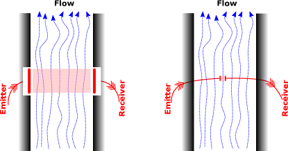
Figure 1: Left: A macroscopic second sound resonator, embedded in the sidewall, is used to sense the averaged flow properties in the shaded region. Right: Second sound tweezers. In contrast to the macroscopic design of the left schematic, this miniaturized resonator, positioned within the flow, allows for space and time resolution of the flow variations.

The characteristics of standard (macroscopic) second sound resonators listed above also apply to their miniaturized counterparts, named second sound tweezers. In addition to their smaller size, a key feature of tweezers is their minimal impact on the flow when positioned in its core. This is illustrated in Figure 1, which highlights the differences between standard resonators and tweezers. Standard resonators provide information on the averaged properties of the flow, while tweezers enable space and time-resolved measurements. As such, tweezers function as local probes, similar to hot-wire anemometers or cold-wire thermometers used in turbulence studies.

The present design for tweezers utilizes thermal actuation, which is preferred over mechanical actuation due to its compatibility with the constraints of miniaturization and reduced flow blockage.

I.4 Overview of the manuscript

The following sections cover distinct topics.

In Section III, we present a comprehensive model of second-sound resonators that accounts for plate misalignment, advection, finite size, and near-field diffraction. Diffraction, which was previously neglected in quantitative models, is shown to be a significant source of degradation of the quality factor in our case studies. We also consider applications of this model for the measurement of vortex concentration or velocity.

In Section IV, we discuss existing methods for processing the signal from second-sound resonators and their limitations. To overcome these limitations, we introduce a new general approach, called the elliptic method, based on mathematical properties of resonance. This method enables us to dynamically separate the amplitude variations of the standing wave due to variations of vortex density or velocity from the phase variations, such as those resulting from variations of the second sound velocity due to a temperature drift.

In Section II, we report on the design, clean-room fabrication, and operation of miniaturized second-sound resonators called. These tweezers allow us to probe the throughflow of helium with unprecedented spatial and time resolution.

To ensure clarity, we present the second-sound tweezers first to illustrate the topics on modeling and methods with a practical case. However, we emphasize that the modeling and methods introduced in this article are general and relevant to second-sound resonators, regardless of their size, including the macroscopic sensors embedded in parallel walls that are encountered in the literature.

II Design, fabrication and mode of operation of second sound tweezers

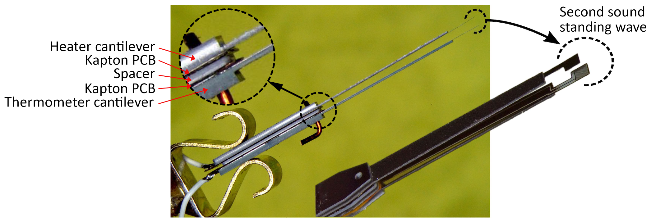
Figure 2: Second sound tweezers, pictured from two angular perspectives. Center: The probe is seen in the direction of the mean flow (or nearly so). The second sound cavity is localized at the end of the probe tip, in the rightmost encircled areas. The bent copper wire passing through the probe is a temporary joystick used for precise alignment of the cavity plates under the microscope. The two coaxial cables for heating and thermometry are visible in the lower left corner of the picture. Top left: Magnified detail of the stack. Right: The picture insert shows the same probe after rotation, and with the joystick removed, revealing the through-hole across the silicon stack. The two staggered notches used for thermal confinement of the standing wave in the cavity are clearly visible.

The basic component of second sound tweezers consists of a stack comprising a heating cantilever and a thermometer cantilever, separated by a spacer. Additionally, two Kapton films with golden copper tracks are inserted in contact with the tracks of the heater and thermometer (see Fig. 2). The heaters and thermometers cantilevers are composed of a baseplate, an elongated arm, and a tip (see Fig. 3). The baseplate is the thickest part, while the tip is the thinnest. The active areas, which are the emitter and receiver plates, are located on the tips. The distance between the plates is set by the spacer, composed of one or several micro-machined silicon elements. For a given device, the heater and thermometer have identical mechanical structures, with the only difference being the chemical elements used in the serpentine electrical path deposited on the tip. Three cantilever types were fabricated to allow the assembly of resonators with three different tip sizes (see Fig. 3). The tip widths are 1000 µm, 500 µm, and 250 µm. The resulting assembly is clamped with a standard picture clip, which was downsized in width by electro-wire erosion, and soldered to the head of a mounting screw. An improvement compared to the clamping technique introduced in RDD⁺, 07 is the possibility to insert a temporary "joystick" through the entire assembly to allow for precise alignment (or offsetting) of the cavity plates under a microscope.

Next subsection II.1 presents the considerations that have prevailed in the mechanical design of the second sound tweezers. The following section, II.2, discusses the detection (thermometry) and generation (heating) of second sound by the tweezers. The last two subsections present the microfabrication techniques (section II.3) and the electrical circuitry used to operate the probes (section II.4).

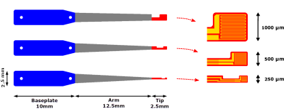
Figure 3: Top view of the 3 cantilever types. The tips widths are respectively 1000 µm, 500 µm and 250 µm. Left: Mechanical structures, all parts are silicon made, different thicknesses are represented by different colors. The baseplate width is 2.5 mm for all types. Right: Electrical path on each tip type. Yellow areas are a deposition of TiPt for heaters and AuSn for thermometers. Orange areas are a thick AuPt deposition for current leads.

II.1 Mechanical design

Resolution. The space resolution of the tweezers, denoted as $L_{\text{res}}$, is determined by the largest dimension of its cavity, which can be either the inter-plates distance $D$, also known as the "gap", or the side length $L$ of the plates which are assumed to be square-shaped. This study mostly focuses on cavities with an aspect ratio of order 1, which allows for optimal space averaging of the signal at a given space resolution. The time resolution of the tweezers, denoted as $\tau_{\text{res}}$, is set by the decay time of a wave bouncing between the plates. In Section III.2, we introduce and validate a simple model that accounts for dissipation in the cavity due to diffraction loss and residual inclination of the plates. An upper bound for $\tau_{\text{res}}$ is obtained from the diffraction loss term: $\tau_{\text{res}}\simeq L^{2}f/bc_{2}^{2}$, where $b\approx 0.38$, where $c_{2}$ is the second sound velocity, and $f$ is the wave frequency, which can be approximated as $nc_{2}/2D$ for the $n^{th}$ mode of resonance (see Eq. 6). Thus, the tweezers time resolution due to diffraction loss can be estimated as

$$\tau_{\text{res.}}\simeq\frac{L^{2}f}{bc_{2}^{2}}\simeq n\frac{L^{2}}{Dc_{2}}$$

The ratio $L_{\text{res}}/\tau_{\text{res}}$ of the space resolution and time resolution defines a characteristic velocity for which the probe optimally averages the space-time fluctuations. For instance, in cavities of aspect ratio one ($D=L$) operated on its $n^{th}$ resonance, the nominal velocity is estimated as $c_{2}/n$. These estimates show that cavities with an aspect ratio of order unity are appropriately sized for second-sound-subsonic flow, with a mean velocity of a few meters per second.

Blocking effect. The aforementioned considerations regarding space resolution are pertinent only if the flow being measured is not disturbed by the probe support. The current design adheres to the empirical $10\times$ rule, which mandates that components of the support that impede the flow on a length scale $\mathcal{X}$ must be situated at least $10\mathcal{X}$ away from the measurement region. Accordingly, the cavity is located at the end of elongated arms, and the cantilevers exhibit decreasing widths and thicknesses along their length of 25 mm, as depicted in Figure 2. The thickness successive values are around 520$\mu m$, 170$\mu m$ and 20$\mu m$ while the width decreases from 2.5mm to $145\>\mu m$ in the narrowest zone (resp. $275\>\mu m$ and $500\>\mu m$) for cavities with $L=250\,\mu m$ (resp. $L=500\,\mu m$ and $L=1000\,\mu m$).

Wave confinement: The spatial resolution of the tweezers would be degraded if the second sound standing wave spread out of the $L\times L\times D$ cavity due to reflections between the supporting arms. To confine the standing wave in the cavity region, a design trick was implemented by breaking the mirror symmetry between the two cantilevers. As shown in Fig. 2, anti-symmetric notches in the tips prevent the second sound from escaping by bouncing away from the cavity, at least in the geometric-optic approximation where diffraction is neglected.

Mechanical resonances. In addition to the $\times 10$ rule, these dimensions are chosen to push the mechanical vibrations of the arm to around $1$ kHz or higher. The fundamental resonance frequency of the trapezoidal-shaped arm in vacuum was estimated using the analytical formula in Lob, 07 (section 1.3.1.1).

$$f_{0}=\frac{8.367}{2\pi}\frac{e}{t^{2}}\sqrt{\frac{E_{Si}(3w_{2}+w_{1})}{\rho_{Si}(49w_{2}+215w_{1})}}$$

We obtain $f_{0}=2195\>$Hz (resp. 1889 Hz and 1569 Hz) using the material properties $E_{Si}=140$ GPa, $\rho_{Si}=2330\>$kg$/$m³, and the dimensions of the intermediate section of the arm having thickness $e=172\>\mu$m, length $t=12.5\>$mm, and width decreasing from $w_{2}=1.5\>$mm to $w_{1}=250\>\mu$m (resp. to $500\>\mu$m and $1000\>\mu$m). An experimental validation was conducted at room temperature in air with an arm having $w_{1}=1000\>\mu$m. Its mechanical vibration frequency spectrum was measured using a photoreceptor that detected a laser beam reflecting off the arm. The mechanical excitation was provided either by tapping the table supporting the set-up with a small hammer or by directing a jet of compressed air toward the arm. In both cases, the fundamental mechanical resonance frequency was found to be 1215 Hz, in reasonable agreement with the predicted value of 1569 Hz given the uncertainty in the Young’s modulus $E_{Si}$ and deviations from the trapezoidal shape. As discussed in Section IV.4.3, indirect measurements of the resonance frequency were conducted in a superfluid flow with a velocity of $1.2$ m$/$s, and gave $f\approx 825$ Hz, $f\approx 1050$ Hz, and an amplitude of vibration smaller than $1\>\mu$m. The decrease in frequency compared to the room-temperature measurement is interpreted as being mostly due to a fluidic added mass effect Sad (98).

Deflection of the tips’ ends.

The thicknesses of the tweezers parts are chosen such that the mechanical deflection at the tip endpoint remains significantly lower than the inter-plate distance under typical operating conditions.

The deflection at the tip endpoint can be estimated by considering separately the arm deflection (with thickness 172$\>\mu$m) and the tip deflection (with thickness 20$\>\mu$m). As a first approximation, both arm and tip are considered as cantilever beams of uniform width submitted to a uniformly distributed load, and having one embedded end and one free end. This geometrical approximation overestimates the deflection of the arm, as its endpoint is narrower than its base, and it underestimates the deflection of the tip, as the notch is ignored. Nevertheless, this provides order-of-magnitude estimates. The load is estimated as the dynamic pressure of a liquid helium flow impinging the tweezers in the transverse direction at a velocity $U=0.1\>$m/s, which is 10% of the typical longitudinal flow velocity of 1 m/s. The dynamic pressure $P$ is given by:

$$P=\frac{1}{2}\rho U^{2}$$

where the liquid helium density is $\rho\simeq 140\>$kg/m³. According to Euler-Bernouilli beam theory, the free end deflection $\delta_{\text{max}}$ of the cantilever is given by:

$$\delta_{\text{max}}=\frac{3}{2}\frac{Pt^{4}}{E_{Si}.e^{3}}$$

The total deflection of the tweezers (arm and tip) can be upper-bounded by considering the sum of the deflection of a 2.5 mm long tip and a 15 mm (not 12.5 mm) long arm. This takes into account the small angle generated on the tip by the arm deflection. Using the values $t=15\>\text{mm}$ (length), $e=172\>\mu\text{m}$ (thickness), and $E_{Si}=140\>\text{GPa}$ (Young’s modulus), the deflection of the arm endpoint is found to be 75 nm, while the deflection of the tip endpoint with $t=2.5\>\text{mm}$ and $e=20\>\mu\text{m}$ gives a deflection of 37 nm. Thus, the total mechanical deflection of the tweezers tip due to a steady lateral flow of 0.1 m/s is a fraction of a micron, which is decades smaller than the inter-plate distance.

The mechanical resonance of the tweezers arm and tip discussed above could lead to deflections larger than those due to steady forcing. The amplitude of these mechanical oscillations was measured in a turbulent He II flow, up to velocities exceeding 1 m/s, taking advantage of the dependence of the second sound resonance with respect to the cavity gap. The measured signal will be presented to illustrate the efficiency of the elliptic projection method in separating the fluctuations of the acoustical path of the cavity and the fluctuations of the bulk attenuation of second sound between plates. The mechanical oscillations of the cavity gap are found to be typically $0.5\>\mu\text{m}$ (around 1 kHz). As expected, such a deflection is decades lower than the interplate distance (1.3 mm in this case) and the second sound wavelength.

Boundary layer. In the presence of a mean flow through the cavity, a velocity boundary layer will develop along the tweezers’ plates. In principle, this boundary layer could contribute to the measured signal and alter the measurement of the incoming flow. For instance, it could increase the density of superfluid vortices in the cavity and therefore affect second sound attenuation. However, as illustrated later, the second sound standing wave that settles between the plates has nodes of velocity near the plates while the sensitivity of second sound to vortices arises in antinodal regions of velocity. As long as the boundary layer thickness is thin enough, say within a fraction of $\lambda/4$ ($\lambda=c_{2}/f$ is the second sound wavelength), it is not expected to significantly alter the measured signal.

A first requirement for this condition is that the mean flow direction is parallel to the plates, so that the flow penetrates through the cavity with minimal deflection. A consequence of this is that the plates should be widely separated when operated in flows with undefined or zero mean velocity, such as the core of a mixing layer.

A second requirement is that the plate thickness is much thinner than $\lambda/4$. The current plates are 20 microns thin, which is much smaller than $\lambda/4\simeq D/2n$ for the $n^{th}$ mode of resonance. For instance, with $D=500\>\mu m$ and $n=3$, the condition $20\ll\lambda/4\simeq 83\>\mu$m is indeed satisfied.

A third condition pertains to the downstream development of the boundary layer thickness, which should also remain within $\lambda/4$. The physics of boundary layers in He II is not yet well-understood SPB (17), but existing experiments (e.g. SHVS, 99) suggest that classical hydrodynamic phenomenology could remain valid in the high-temperature limit. In classical hydrodynamics, the so-called displacement thickness of a laminar Blasius boundary layer at a distance $L$ from its origin is given by

$$\delta_{\text{{bl}}}=1.73\sqrt{\frac{L\nu}{U}}$$

where $U$ is the mean velocity far from the boundary layer and $\nu$ is the kinematic viscosity of the fluid. In He II, several diffusive coefficients could arguably play the role of $\nu$, including the quantum of circulation around a quantum vortex and the kinematic viscosity associated with the dynamics viscosity of the normal fluid normalized either by the normal fluid density or by the total density. In the temperature range of interest, all these diffusive coefficients are within one order of magnitude, typically $10^{-8}-10^{-7}$m²/s. Taking $\nu=3.10^{-8}\>$m²/s, $L=1000\>\mu$m, and $U=0.5\>$m/s, one finds $\delta_{\text{bl}}=13\>\mu$m, and a boundary layer Reynolds number $\delta_{\text{bl}}U/\nu=217$ consistent with the laminar picture. This thickness estimate, similar in magnitude to the plate thickness, satisfies the third requirement $\delta_{\text{bl}}\ll\lambda/4$.

II.2 Second sound detection and generation

II.2.1 Thermometry

The temperature-sensitive material used in the present study is AuSn, which fulfills two requirements: (1) it is compatible with the microfabrication process and (2) it can be tuned to become temperature-sensitive over a range of interest to quantum turbulence studies WVR (21), from 1.5 K up to the superfluid transition temperature $T_{\lambda}\simeq 2.18$ K in saturated vapor conditions. Other materials may be more suitable for other conditions; for example, Al was previously used for tweezers operated around 1.5 K in RDD⁺, 07.

The gold-tin AuSn thermometer is a metal-superconductor composite material, with superconducting Sn islands electrically connected by a gold layer. This granular structure is shown by electron microscopy in Fig. 4 (right). The temperature dependence phenomenology can be interpreted simply. Indeed, by proximity effect, the gold in contact with tin behaves as a superconductor over a spatial extent that depends on temperature. By adjusting the characteristic length scales and thicknesses of the granular pattern, the temperature response of the material can be tuned.

As a preliminary study, the temperature dependence of the resistance of a 100-square-long AuSn track was measured for three different tin thicknesses, as shown in the top plot of Fig. 5. The track resistance is directly proportional to its number of squares (length-to-width ratio of the track) with the sheet resistance as a multiplying factor. A description of the conduction mechanism in AuSn is presented in BSS, 83.

In the present study, the total resistance at superfluid temperatures does not exceed a few hundred ohms. This value was chosen to be much larger than the resistance of the leads, but small enough to prevent parasitic effects from the leads’ capacitance (typically a few hundred picoFarads) up to the highest frequencies of operation.

To achieve resistance values in this range, the meander length was fixed at around 700 squares for all tip sizes. Depending on the tip size, the track width was adjusted so that the serpentine shape occupies the entire available area on the tip. At room temperature, the AuSn layer resistance was found to drift from low values to a final value over the course of a few days (less than one week) after deposition. After this period, the resistance was found to be stable for at least a few years.

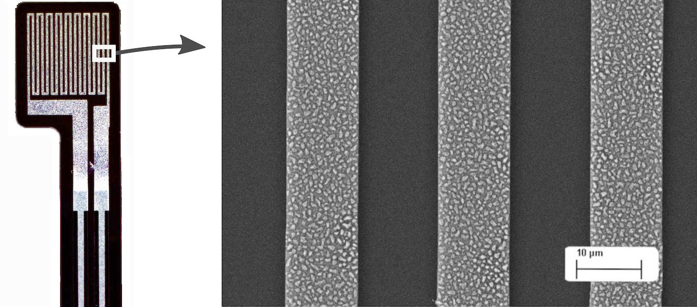
Figure 4: Scanning electron microscope view of a tip. Left: Tip frontside view. The overlaps between the serpentine path material and the current leads are visible on the lower part of the picture. Right: Detail of AuSn layer showing its granular aspect. Depending on tweezers models (see Fig. 3), the width of the AuSn track is 4, 11 or 24 $\mu$m.

Figure 5 (bottom plot) shows a typical resistance-temperature curve $R(T_{0})$ for an AuSn thermometer at different direct currents $I$. Regarding the temperature dependence of resistance, the current density is a more significant parameter than the total current. Thus, the comparison between the top and bottom plots of Figure 5 should be made at constant values of the ratio of current to track width. At low current densities ($I\leq 10\mu A$), the sensitivity exceeds $1\>\varOmega.$mK^-1. At larger current densities, the current-induced magnetic field significantly shifts the superconducting-metal transition to lower temperature and broadens it, allowing the measurement range to be extended down to 1.6 K and below. In the range of currents explored in Figure 5, the reduction in sensitivity in $\varOmega.$K^-1 at larger currents $I$ is more than compensated by the larger sensitivity in V.K^-1 units across the thermistor. Most measurements presented hereafter are performed with a measuring current $I\simeq 27\>\mu$A.

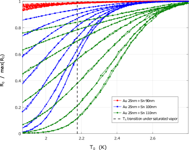
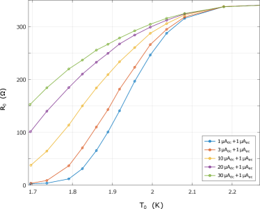
Figure 5: Top: Example of temperature and current dependence of AuSn layers with different Sn thicknesses deposited on a track of width $50\>\mu$m. The current setpoint spans from $1\>\mu$A up to $1$ mA. Bottom: Temperature response of the AuSn track of small tweezers for different electrical currents. The thickness of the tin layer is 100 nm of Tin, and the width of the track is $4\>\mu$m. The small difference between both plots -when compared at similar current densities- is compatible with the uncertainty on the layer thicknesses. This good agreement indicates that AuSn properties are robust to the full fabrication process of the tweezers.

II.2.2 Heating

The heater has the same meander length as the thermometer, which is close to 700 squares for all tip sizes.

As shown in Figures 3 and 4, a buffer zone was designed between the gold tracks and the meander. In this zone, the electrical path is wide, but the material is the same as in the meander (platinum for the heater). The buffer zone’s length is approximately 20 squares, aiming to provide some thermal insulation between the meander and the gold track.

Numerous resistive materials are suitable for this purpose. For instance, chrome was used for the tweezers in RDD⁺, 07, and platinum was used in WVR, 21. The present data were obtained with platinum to benefit from the temperature-independence of its resistivity at superfluid temperatures PK (82) and also allow reusing these miniature heaters as miniature thermometers or hot-film anemometers in experiments conducted at higher temperatures where Pt regains temperature dependence Kem (91). A 5 nm titanium layer was deposited before platinum as an adhesion layer.

The thickness of the Pt layer, around 80 nm, was chosen to ensure that the electrical resistance of the heater at superfluid temperatures is on the order of a few hundred ohms, similar to the maximum resistance of the thermometer and for the same reasons.

The heater is driven with a sinusoidal current at a frequency of $f/2$. The resulting Joule effect can be separated into a constant mean heating and a sinusoidal heat flux at frequency $f$, which drives the second sound resonance. One advantage of this $f/2$ excitation is that the signal detected by the thermometer, centered around $f$, is not affected by spurious electromagnetic coupling at $f/2$ from the excitation circuitry. Thus, no special care is needed to minimize the electromagnetic cross-talk between the electrical tracks of the heater and the electrical tracks of the thermometer, despite their proximity.

The non-zero mean heating results in a steady thermal flux in He II, with the corresponding entropy carried away from the heater in the form of steady normal fluid flow. This outgoing normal flow is balanced by an opposite steady mass flow of superfluid toward the heater. Such cross-flows are referred to as counterflows in the quantum fluid literature Tou (82); NF (95). This steady counterflow adds up to a pure second sound generated by the heater, but contrary to it, its effects are not amplified by resonance in the cavity.

Quasi-linear vs non-linear regimes: The second sound resonators are operated with standing waves of low amplitude, typically around $\sim 100\>\mu$K. In this regime, the amplitude $T$ of the temperature standing wave responds nearly linearly to the heating power $P$. However, for larger heating power, the ratio $T/P$ decreases with $P$, indicating a turbulent transition within the tweezers that leads to a dense tangle of quantum vortices dissipating the second sound wave. The crossover from the quasi-linear to non-linear response of $T(P)$ is shown in Figure 6 (left plot) for tweezers at 1.6 K in the absence of external flow. In these conditions and for these tweezers, the transition occurs around $P\simeq 1$ W/cm², where $P$ is the total Joule power normalized by the heating surface. In other conditions, the transition was observed at smaller power densities, but no systematic study has been carried out to determine the threshold value.

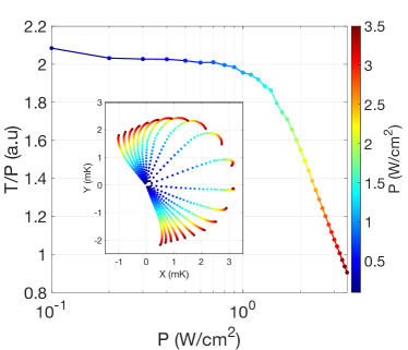
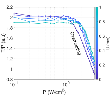
Figure 6: Left: The normalized amplitude $T/P$ of the temperature standing wave versus heating power $P$ is shown for second sound tweezers in quiescent He II around 1.6 K. The transition around $P=1$ W/cm² is interpreted as the development of a self-sustained vortex tangle within the probe. The inset shows the amplitude of the temperature standing waves in the complex plane for a subset of frequencies belonging to the same second sound resonance. In this representation, the extra-dissipation associated with the self-sustained vortex tangle results in a curvature of the iso-frequency radial "lines", revealing the broadening of the resonance. Right: The same quantity is shown for second sound tweezers swept by turbulent flows of different mean velocities but similar turbulence intensity. In the linear regime $P\lesssim 1$ W/cm², the velocity dependence is opposite to that in the non-linear regime, $P\gtrsim 2$ W/cm², demonstrating respectively vortex and velocity sensing by the probe.

II.2.3 Digression on the operation in the non-linear heating regime

The current study primarily focuses on the linear regime of heating, but a brief investigation of higher powers reveals an interesting property of non-linear operation and supports the above interpretations of the nature of the non-linear regime. Figure 6-right displays the amplitude of the normalized temperature standing wave $T/P$ versus $P$ in flows with different mean velocities $U$ and turbulence intensity of a few percent. In the linear regime ($P\apprle 1\>$W/cm² in the conditions of Fig. 6), the plateaus of $T/P$ decrease as $U$ increases, in accordance with the classical interpretation (discussed later) that the standing wave $T$ is damped by the vortices present in the external flow, whose concentration increases with $U$. Interestingly, in the non-linear regime (around $P\apprge 2\>$W/cm² in Fig. 6), the dependence of $T/P$ on $U$ is opposite. The interpretation is that the extra damping of the standing wave $T$ is mainly due to the vortices generated within the tweezers by the heating itself. This vortex density decreases at higher $U$ because vortices are more effectively swept out of the tweezers. Thus, in the non-linear regime, the second-sound tweezers behave as local anemometers. In the linear regime, we will demonstrate that second-sound tweezers can not only act as vortex probes (as shown in Fig. 6-right), but also as anemometers through a mechanism discussed later.

II.2.4 Thermal load of the tip on the fluid

The specific heat of the cantilever tip, mostly made of silicon Des (86), is much smaller than the specific heat of a similar volume of liquid helium at the temperature of interest. For instance, at the intermediate temperature of 1.8 K, they differ by more than 5 orders of magnitudeOP (94); DB (98) with $C_{p}^{Si}\simeq 3.5$ J.K^-1.m^-3 while $C_{p}^{LHe}\simeq 4.3\times 10^{5}$ J.K^-1.m^-3.

The thermal resistance of the interface between the tip and the fluid can be estimated from the literature on the Kapitza resistance (Pol, 69; RVA, 16 and references within). At a given temperature, this resistance depends on the tip surface material (Pt, AuSn, SiO₂ or Si), on the surface roughness and cleanliness, and on the normal/superconducting state of the material. Based on values reported in Pol (69); JL (63); OP (94), the tip-helium thermal resistance at 1.8 K is estimated to be within $1-6$ cm².K.W^-1 on each side.

The characteristic response frequency $\left(2\pi RC\right)^{-1}$, where $R=3$ cm².K.W^-1 is the typical Kapitza resistance and $C=e\cdot C_{p}^{Si}$ with $e=20$ $\mu$m is the thermal inertia of the cantilever tip per surface unit, exceeds 7 MHz at 1.8 K. This frequency is significantly larger than the largest frequencies of the second sound considered here. As the Kapitza resistance roughly scales as $T^{-3}$ and the tip inertia as $T^{3}$, this characteristic frequency does not strongly depend on temperature.

The estimates above illustrate the negligible thermal load of the probe compared to the surrounding fluid and its ability to respond to rapid environmental fluctuations. Previous studies have reported measurements extending over a bandwidth of 1 MHz or higher, not only in superfluids (e.g. see CSW, 78) where helium’s high thermal conductivity benefits the fluid-probe system’s dynamics, but also in gazeous heliumCCH (92); CCCH (00); PPB⁺ (03), where the system’s thermal inertia is determined by the fluidic boundary layerGSB⁺ (09).

Deriving the full transfer functions for the coupling between the second sound standing wave and the probe would require a detailed thermal analysis beyond the scope of this paper. Instead, our approach was to assume an ideal response of the probe and to show that the resulting analytical predictions closely match experimental measurements.

II.3 Microfabrication and assembling

The mechanical structures of the cantilevers and spacers are made of silicon. The cantilevers were fabricated by processing SOI (Silicon On Insulator) wafers by microelectronic techniques. SOI wafers consist of a thin silicon layer (known as the device layer) separated from a thick silicon substrate by an insulator layer, which in this case is a buried oxide with a thickness of 1 µm. The device layer has a thickness of 20 µm, while the silicon substrate layer is 500 µm thick. Standard photolithography was used to create the metal and silicon shapes. The diameter of the wafers was 100 mm. As shown in Fig. 7, the patterns for the 46 cantilevers on each wafer were arranged radially, with the cantilever tips positioned close to the wafer center to ensure higher reproducibility of the tip properties. The wafers were double-side polished and oxidized to create a 100 nm thick SiO₂ layer on both sides.

A simplified version of the cantilever fabrication process is presented in Table 1, with full details provided in the appendix. The serpentine electrical path (colored red) was deposited first on the frontside of the SOI wafer. For heaters, the evaporation sequence Ti 5 nm + Pt 80 nm was used, while for thermometers (assuming a hypothetical thickness for a planar - not granular - tin layer), Au 25 nm + Sn 100 nm was used. During a second sequence, current leads (colored orange) were deposited, with an evaporation sequence of Ti 5 nm + Au 200 nm + Ti 5 nm + Pt 50 nm. The use of a platinum layer was found to facilitate lift-off and may also be useful for brazing purposes.

The cantilevers’ 3D shape was achieved through the use of an STS HRM deep reactive ion etching (DRIE) tool, employing recipes based on the technology known as "Bosch process". This tool is capable of etching silicon to a depth of several hundred microns with perpendicular sidewalls. Non-etched regions were protected by resist or aluminum layers. By using various etching recipes and protecting layers (resist, aluminum, and silicon oxide), the silicon was initially etched from the backside with two different mask shapes, followed by the frontside to achieve silicon plate piercing. The resulting pieces had tip areas made up of the original 20 µm thick SOI device layer, with the 1 µm thick oxide removed from the tip backside to avoid bending due to oxide mechanical stress. While some spacers were fabricated together with the cantilevers, most of them were made separately from two silicon wafers with thicknesses of 300 µm and 525 µm, coated by thin dielectric layers on both sides.

Figure 7: Overview of mask design. The disk diameter is 100 mm.

Step	Cut view
1. SOI wafer (surface oxide 0.1 µm / silicon device 20 µm / buried oxide 1 µm / silicon substrate 500 µm / surface oxide 0.1 µm).
2. Electrical circuitry fabrication.
3. Backside etching 1.
4. Backside etching 2.
5. Frontside etching mask fabrication.
6. Frontside etching and mask removal.

Table 1: Cantilevers fabrication process.

II.4 Electric circuit

Figure 8 depicts the circuit utilized for time-resolved measurements using second-sound tweezers, including example values for resistances and gain. The time-resolved data presented in this paper were obtained using this circuit and the following equipment. The front-end preamplifier is either the Celian EPC1-B model or the NF SA-400F3 model when exploring frequencies above 100 kHz. The lock-in amplifier is the NF LI-5640 model or the SignalRecovery Model 7280 above 100 kHz. In most cases, the lock-in amplifier’s built-in internal generator provides both the drive for the tweezers’ heater (at frequency $f/2$) and the reference frequency to detect the temperature signal (at frequency $f$). The acquisition system is based on the National Instrument PXI-4462 analog input cards, and it records both the in-phase ($X$) and quadrature ($Y$) signals from the lock-in amplifier’s analog outputs.

In certain situations, the temperature signal at the lock-in input is overwhelmed by a much larger electromagnetic parasitic signal at $f/2$, and it cannot be accurately resolved by the limited voltage dynamic range of the lock-in amplifier. This can happen when the tweezers are operating far from resonance, where the second-sound signal is small, or when the tweezers are operating at very high frequencies (e.g., > 100 kHz), as electromagnetic parasitic coupling increases with frequency. The magnitude of this parasitic coupling is determined by the tweezers and cable’s geometrical and electrical characteristics. Within the range of parameters investigated in this study, the order of magnitude of the parasitic voltage induced across the thermometer resistor, normalized by the voltage applied across the heating resistor, is given by

$$0.5\%\times\frac{{f}/{2}}{100\>\text{kHz}}$$

Such situations are handled thanks to the differential input of the lock-in amplifier, which removes a signal mimicking the parasitic one. In such cases, a two-channel waveform generator is used: one channel drives the heater (at frequency $f/2$), another channel mimics the parasitic signal (at frequency $f/2$, with manually tuned amplitude and phase shift), and the "sync" output of the generator synchronizes the lock-in demodulation (at frequency $f$). The Agilent 33612A generator is used for this purpose. Alternatively, the compensation signal can be generated directly from the lock-in internal generator, completed with a simple RC phase shifter and, eventually, a ratio transformer.

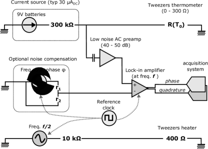
Figure 8: Example of circuitry for measurements with a high dynamical reserve.

In principle, any thermistor with a positive temperature coefficient, such as an transition-edge thermometer, that is not well thermalized with the fluid can become unstable when driven by a current source. An infinitesimal thermistor fluctuation from $T_{0}$ to $T_{0}+\delta T_{0}$ leads to a resistance variation of $\delta R=\frac{\partial R}{\partial T_{0}}.\delta T_{0}>0$, resulting in an excess of Joule dissipation $\delta R.I^{2}$ for a constant current drive $I$. Let $\mathcal{R}_{th}$ be the thermal resistance of the thermistor-fluid interface, then this extra Joule dissipation results in an overheating of $\mathcal{R}_{th}\times\delta R.I^{2}$, which could lead to a thermal instability. The stability condition is difficult to predict for a spatially distributed thermistor deposited on a Si crystal and immersed in superfluid. Thus, initial tests were done with a voltage drive before empirically validating the stability of our current drive.

The frequency bandwidth of the measurements is arbitrarily set by the integration time constant of the lock-in amplifier. In practice, the circuit’s performance is limited by the input voltage noise of the EPC1-B pre-amplifier, which is $0.65\>$nV/$\sqrt{\text{Hz}}$. For a current drive of $27\>\mu\text{A}$, a thermometer sensitivity of $0.5\>\Omega\cdot\text{mK}^{-1}$, and a demodulation bandwidth of 10 Hz or 1000 Hz, the temperature resolution $T_{rms}$ is given by:

$$T_{rms}=\frac{\sqrt{10}.0.65}{0.5\times 27}\mu\>\text{K}\simeq 150\>\text{nK}$$

for a 10 Hz measurement bandwidth, or

$$T_{rms}=\frac{\sqrt{1000}.0.65}{0.5\times 27}\mu\text{K}\simeq 1.5\>\mu\text{K}$$

for a 1 kHz measurement bandwidth

These resolutions are sufficient under standard conditions. They are three and two orders of magnitude smaller, respectively, than the typical amplitude of second sound at resonance. Reaching the same temperature resolution at a significantly larger bandwidth would be futile, given the spatiotemporal resolution of the probe itself. If necessary, better resolution could be achieved with a larger current across the thermometer or by using a cryogenic amplifier (e.g., see DLF⁺, 14 and http://cryohemt.com) before being limited by the thermal noise floor of the thermistor (typically $0.15\>$nV/$\sqrt{\text{Hz}}$ for $200\>\varOmega$ at 2 K).

III Models of second sound resonators

The second sound equations within the linear approximation can be written in terms of the temperature fluctuations $T$ and the velocity of the normal component $\mathbf{v}_{n}$ as

$$\partial_{t}\mathbf{v}_{n} +\frac{\sigma\rho_{s}}{\rho_{n}}\nabla T=0,$$ (1)

$$\partial_{t}T +\frac{\sigma T_{0}}{c_{p}}\nabla.\mathbf{v}_{n}=0.$$

with $\sigma$ the entropy per unit of mass, $c_{p}$ the heat capacity, and $\rho_{s}$ , $\rho_{n}$ are the densities of the superfluid and normal components respectively. All along the present section, $T_{0}$ is the notation for bath temperature far away from the tweezers. $T$ denotes the local temperature fluctuations, that depend both on space and time. From this definition, we obviously have $\left\langle T\right\rangle=0$ where $\left\langle\right\rangle$ is the time average.

We introduce the second sound velocity $c_{2}$ defined by the relation

$$c_{2}^{2}=\frac{\rho_{s}}{\rho_{n}}\frac{\sigma^{2}T_{0}}{c_{p}}.$$ (2)

It can be deduced from Eqs. (1) that both the temperature $T$ and the normal velocity $\mathbf{v}_{n}$ follow the wave equation

$$\partial_{t}^{2}T-c_{2}^{2}\Delta T=0.$$ (3)

We explain in the present section how Eqs. (1-2-3) can be used to build quantitative models of second sound resonators. We first focus on phenomenological aspects in sec. III.1. Then, we give analytical approximations in sec. III.2 and an accurate numerical model in sec. III.3. Finally, we discuss the model quantitative predictions in secs. III.4 and III.5.

III.1 Resonant spectrum of second sound resonator: phenomenological aspects

The basic idea of second sound resonators is to create a second sound resonance between two parallel plates facing each other. A second sound wave is excited with a first plate, while the magnitude and phase of the temperature oscillation is recorded with the second plate, used as a thermometer. For simplicity, we assume from now on that the second sound wave is excited by a heating, but the whole discussion can be straightforward extended to nucleopore mechanized resonators. The temperature oscillations within the cavity are coupled to normal fluid velocity oscillations according to the second sound equations (1).

We note $j_{Q}=j_{0}e^{2i\pi ft}$ the periodic component of the heat flux emitted from the heater. We assume throughout the present article perfectly insulating plates, which means that the boundary conditions for the second sound wave are

$$\mathbf{v}_{n}.\mathbf{n}=\begin{cases}0&\text{for }z=D\\ \frac{j_{Q}}{\rho\sigma T_{0}}&\text{for }z=0\end{cases},$$ (4)

where $\mathbf{n}$ is the unit vector directed inward the cavity and normal to the plates. The second equation in (4) reflects the fact that the normal component carries all the entropy in the fluid. According to the first relation in Eq. (1), the boundary conditions (4) for the normal velocity translate into the following boundary conditions for the temperature field

$$\nabla T.\mathbf{n}=\begin{cases}0&\text{for }z=D\\ -\frac{\rho_{n}\partial_{t}j_{Q}}{\rho\rho_{s}\sigma^{2}T_{0}}&\text{for }z=0\end{cases}.$$ (5)

We display in Fig. 9 a typical experimental spectrum of second sound tweezers, that is, the temperature magnitude averaged over the thermometer plate, as a function of the heating frequency $f$. The spectrum is reminiscent of that of a Fabry–Perot resonator: it displays very clear resonant peaks that are almost equally spaced, and a stable non-zero minimum at non-resonant frequencies. However, the spectrum of Fig. 9 displays three major characteristics that can be observed for every tweezers’ spectrum. First, the locations of the resonant frequencies are slightly shifted compared to the standard values $f_{n}$ given by $\frac{2\pi f_{n}D}{c_{2}}=n\pi,(n\in\mathbb{N})$ expected for an ideal Fabry–Perot resonator. Only for large mode numbers do the resonant peaks again coincide with the expected values. Second, the temperature magnitude vanishes in the zero frequency limit, and the first modes of the spectrum roughly grow linearly with $f$. In between, the resonant amplitudes saturate and then slowly decrease at high frequency.

These latter peculiarities of the frequency response were not described in previous references about second sound resonators. This prompted us to study different models for second sound resonators, including the finite size effects and near-field diffraction phenomena. We first describe analytical approximations in sec. III.2, then we develop in sec. III.3 a numerical algorithm based on the exact solution of the wave equation (3). The numerical scheme can be adapted for various types of planar second sound resonators. We then give quantitative predictions specifically for the response of second sound tweezers without and in the presence of a flow in sec. III.4 and a summary of the main results in sec. III.5.

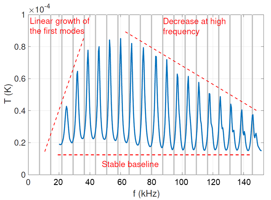
Figure 9: Experimental spectrum of second sound tweezers of lateral size $L=1$ mm and gap $D\approx 1.435$ mm. $f$ is the heating frequency, and $T$ is the thermal wave magnitude. The figure displays the main characteristics of tweezers typical spectrum: first, the resonant frequencies are not located at the values $f_{n}$ given by $\frac{2\pi f_{n}D}{c_{2}}=n\pi,(n\in\mathbb{N})$, displayed by the gray vertical lines. The amplitudes of the resonant modes first increases linearly with $f$ until they saturate and eventually decrease at high frequency. The baseline level only weakly depends on $f$.

III.2 Analytical approximations

The starting point to build our model of second sound tweezers is to assume that all zeroth order physical effects observed with the tweezers are geometrical effects of diffraction. This means in particular that we assume perfectly reflecting resonator plates, and we also neglect bulk attenuation of second sound waves when the fluid is at rest CR (83); RG (84). These assumptions turn to be self-consistent, because the predictions of the model developed in sec. III.3 reproduce the main features observed in experiments.

Second sound resonators embedded in infinite walls

We first consider a finite-size heater and a thermometer of size $L$ embedded in two parallel and infinite walls facing each other. This geometry is most commonly encountered in the literature. With such a configuration, the thermal wave is not a plane wave any more because it is emitted by a finite size heater. The model thus contains diffraction effects. An illustration of the model setup is displayed in Fig. 10. An exact solution of the wave equation Eq. (3) can be found using the technique of image source points. Let $\Sigma_{1}$ be the heating plate and $\Sigma_{2}$ be the thermometer plate, and we assume that the thermometer is sensitive to the average temperature over $\Sigma_{2}$. Then the response of the tweezers is given by $T(t)=\mathcal{R}e\left(\overline{T}e^{2i\pi ft}\right)$ with

$$\overline{T}=\frac{ikj_{0}}{2\pi\rho c_{p}c_{2}}\frac{1}{L^{2}}\iint_{\Sigma_{2}}{\rm d}^{2}\mathbf{r}_{2}\iint_{\Sigma_{1}}{\rm d}^{2}\mathbf{r}_{1}G\left(\mathbf{r}_{2}-\mathbf{r}_{1}\right),$$

with the Green function $G(\mathbf{r})$ defined for every vector $\mathbf{r}$ in the $(x,y)$ plane Goo (05)

$$G(\mathbf{r})=2\stackrel{{\scriptstyle[}}{{n}}=0]{+\infty}{\sum}\frac{1}{\left|(2n+1)D\mathbf{e}_{z}+\mathbf{r}\right|}e^{-ik\left|(2n+1)D\mathbf{e}_{z}+\mathbf{r}\right|}.$$

Such a model correctly predicts that the tweezers’ spectrum vanishes when the heating frequency $f$ goes to zero. Yet, it does not reproduce a linear increase of the resonant magnitude of the first modes, neither the decrease of the resonant peaks at large frequency observed in experiments with second sound tweezers. This means that other effects have to be taken into account to model a fully-immersed open resonant cavity, such as non-perfect plates alignment and energy loss by diffraction outside the cavity when the latter is not embedded in infinite walls.

Empirically modified Fabry–Perot model

The Fabry–Perot model corresponds to a one-dimensional resonator composed of two infinite parallel plates separated by a gap $D$. In that case, the wave Eq. (3) together with the boundary conditions Eqs. (5) can be solved exactly, for a periodic heating $j_{Q}=j_{0}e^{2i\pi ft}$ to find the (complex) temperature $\overline{T}$ at the thermometer plate Ben (22)

$$\overline{T}=\frac{A}{\sinh\left(i\frac{2\pi fD}{c_{2}}+\xi D\right)},$$ (6)

where $\xi$ (in m^-1) is an empirical dissipation coefficient and $A=-\frac{j_{0}}{\rho c_{p}c_{2}}$. An illustration of a Fabry–Perot spectrum is displayed in grey in Fig. 12, with $\xi D=0.15$ and $A=1$. We introduce the wave number $k=\frac{2\pi f}{c_{2}}$. For the simple Fabry–Perot model of Eq. (6), all the resonant peaks have equal height and are uniformly separated. Therefore, some main features of experimental spectra are missing, an indication that important other physical effects have to be included in the model.

Contrary to a Fabry–Perot resonator composed of infinite plates, second-sound resonators are built with plates of finite size $L$, approximately of the same order as the gap $D$ between them. Those finite size effects are important as they introduce a frequency-dependent energy diffracted outside the cavity. This mechanism is sketched in Fig. 10. According to standard diffraction theory, a finite wave initially of size $L$ with a wavelength $\lambda=\frac{c_{2}}{f}$ spreads with a typical opening angle given by $\frac{\lambda}{L}$. By this geometrical effect, a part of the wave energy is lost as the wave reaches the other side of the cavity. The energy loss is roughly proportional to the surface of the wave cross-section that “misses” the reflector (see the right panel of Fig. 10). Therefore, the fraction of energy lost at the wave reflection is controlled by the ratio

$$\frac{\left(L+\frac{2\lambda D}{L}\right)^{2}-L^{2}}{\left(L+\frac{2\lambda D}{L}\right)^{2}} \approx 4\frac{\lambda D}{L^{2}},$$ (7)

$$\approx\frac{4}{N_{F}},$$

where we have introduced the Fresnel number

$$N_{F}=\frac{L^{2}}{\lambda D}.$$ (8)

The tweezers plates are mounted at the top of arms of a few millimeters. The perfect parallelism of the plates is usually not reached for our tweezers, but a small inclination $\gamma$ of the order of a few degrees can be observed instead. A relative inclination $\gamma$ -even small- of both plates creates an additional energy loss mechanism (see Fig. 11). Intuitively, this second mechanism is controlled by the non-dimensional number

$$N_{i}=\frac{\lambda}{\gamma L}.$$ (9)

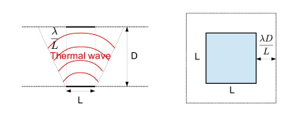
Figure 10: Representation of the wave dispersion. The left picture is a top view parallel to the plates, and the right figure represents a front view of a tweezer’s plate The energy loss is controlled by the non-dimensional number $\frac{\lambda}{L}$, according to standard diffraction theory. In this section, we discuss both the case of tweezers embedded in walls, and the case of free tweezers in open space.

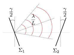
Figure 11: Effect of the plates’ inclination $\gamma$. Inclination creates an additional energy loss mechanism controlled by the second non-dimensional number $\frac{\lambda}{\gamma L}$.

We assume that the Fabry–Perot model (6) can be corrected using the two non-dimensional numbers $N_{F}=\frac{L^{2}f}{c_{2}D}$ in Eq. (7) and $N_{i}=\frac{c_{2}}{\gamma fL}$ in Eq. (9). More precisely, based on empirical observations, we find that second-sound tweezers spectra can be accurately represented by the formula

$$\overline{T}=\frac{A}{\sinh\left(i\left(\frac{2\pi fD}{c_{2}}-a\frac{c_{2}D}{L^{2}f}\right)+b\frac{c_{2}D}{L^{2}f}+c\left(\frac{\gamma fL}{c_{2}}\right)^{2}\right)},$$ (10)

where $a,b$ and $c$ are empirical coefficients. Based on comparison with the full numerical model, we find that the values $a\approx 0.95$, $b\approx 0.38$ and $c\approx 1.3$ give accurate spectra predictions. An illustration of a modified Fabry–Perot spectrum with Eq. (10) is given in Fig. 12. The linear amplitude growth of the first resonant peaks can be interpreted as a progressive focalization of the wave, and is thus controlled by the Fresnel diffraction number $N_{F}$ in Eq. (10). The shift proportional to $\frac{1}{f}$ in peaks frequency positions, observed in the experimental spectra, is also controlled by $N_{F}$. The decrease in resonant magnitude for large mode numbers can be interpreted as a wave deflection outside the cavity, after back and forth propagation between the plates. This latter effect is controlled by the second non-dimensional number $N_{i}$ in Eq. (9).

The major interest of the Fabry–Perot model is to offer an analytical expression to fit locally a resonant peak of a second sound resonator spectrum. The local fit of a peak is of particular interest to interpret the experimental data, as will be explained in sec. IV. Based on Eq. (10), given a measured resonant frequency $f_{0}$, we will look for a fitting expression

$$\overline{T}=\frac{A}{\sinh\left(i\frac{2\pi(f-f_{0})D}{c_{2}}+\xi_{0}D\right)},$$ (11)

valid for second sound frequencies $f$ close to $f_{0}$. In that expression, $\xi_{0}$ encapsulates the different geometrical mechanisms responsible for energy loss when the fluid is at rest. $A$ and $\xi_{0}$ are thus fitting parameters that can be found easily with the experimental data obtained by varying $f$ in the vicinity of $f_{0}$.

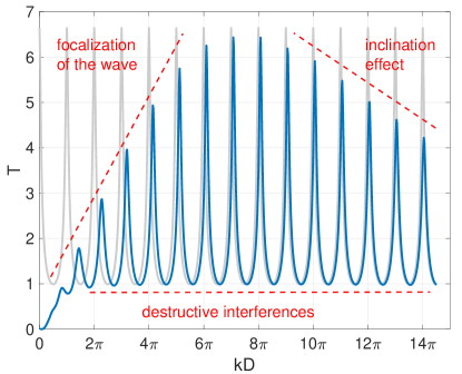
Figure 12: Analytical models of second-sound tweezers. The grey curve represents the standard Fabry-Perot spectrum. The blue curve represents the empirical correction of the Fabry-Perot formula using the two non-dimensional numbers $\frac{\lambda}{L}$ and $\frac{\lambda}{\gamma L}$. The modified spectrum displays the characteristic features of a tweezers experimental spectrum, as displayed in Fig. 9.

III.3 Numeric algorithm

We develop in the present section a numerical algorithm, based on the exact resolution of the wave equations with the particular tweezers’ geometry, with and without flow. The algorithm could be extended to any second sound resonator with a planar geometry. As will become clear in the following, this numerical model allows going far beyond the approximate models of sec. III.2.

III.3.1 For a backgroud medium at rest

The aim of the present section is to build a numerical algorithm to solve the wave equation (3) for a periodic heating $j_{Q}=j_{0}e^{2i\pi ft}$. We look for a solution with the ansatz $T(\mathbf{r},t)=\mathcal{R}e\left(\overline{T}(\mathbf{r})e^{2i\pi ft}\right)$. Then, the wave equation for $\overline{T}$ is

$$\Delta\overline{T}+k^{2}\overline{T}=0,$$

where we have introduced the wave number $k=\frac{2\pi f}{c_{2}}$. The boundary conditions are

$$\begin{cases}\nabla\overline{T}(\mathbf{r}).\mathbf{n}_{1}=-\frac{ikj_{0}}{\rho c_{p}c_{2}}&\text{for }\mathbf{r}\in\Sigma_{1}\\ \nabla\overline{T}(\mathbf{r}).\mathbf{n}_{2}=0&\text{for }\mathbf{r}\in\Sigma_{2}\end{cases},$$ (12)

where $\Sigma_{1}$ is the heater plate and $\Sigma_{2}$ the thermometer plate. The temperature fluctuations have to vanish far away from the tweezers, which implies $T\rightarrow 0$ when $\mathbf{r}\rightarrow\infty$. The notations are given in Fig. 13. We propose the method described below, based on the Huyggens–Fresnel principle. The principle states that every point of the wave emitter can be considered as a point source. The linearity of the wave equation can then be used to reconstruct the entire wave by summation of all point source contributions. The Huyggens–Fresnel principle has been widely used in the context of electromagnetism, for example to compute diffraction patterns produced by small apertures, or interference patterns… The major difficulty in the context of second sound tweezers is that none of the standard approximations of electromagnetism can be done, neither the far-field approximation nor the small wavelength approximation. This explains why numerical resolution is very useful in this context.

We neglect the tweezers arms, which means that both plates are considered as freestanding, infinitely thin and perfectly insulating plates. We allow a relative inclination $\gamma$ around the $x$-axis and a possible relative lateral shift $X_{sh}$ of one plate with respect to the other along the $x$-axis. We assume that the thermometer is sensitive to the temperature averaged over $\Sigma_{2}$.

Let us introduce the Green function

$$G(\mathbf{r})=\frac{1}{\left|\mathbf{r}\right|}e^{-ik\left|\mathbf{r}\right|},$$ (13)

which is the fundamental solution of the wave equation

$$\Delta G+k^{2}G=4\pi\delta(\mathbf{r}).$$ (14)

Let $\Sigma$ be one of our two square plates, and $U(\mathbf{r}^{\prime})$ be a smooth function defined over $\Sigma$. We introduce the wave defined by

$$\overline{T}(\mathbf{r})=\frac{-1}{2\pi}\iint_{\Sigma}G(\mathbf{r}-\mathbf{r^{\prime}})U(\mathbf{r^{\prime}})\;{\rm d^{2}\mathbf{r}^{\prime}}.$$ (15)

By linearity, $\overline{T}$ is a solution of Eq. (3), for all $\mathbf{r}\notin\Sigma$, because $G$ is a solution. An asymptotic calculation in the vicinity of $\Sigma$ then shows that $\overline{T}$ satisfies the boundary condition

$$\nabla\overline{T}(\mathbf{r}).\mathbf{n}\underset{\mathbf{r}\rightarrow\mathbf{r}_{0}\in\Sigma}{\longrightarrow}U(\mathbf{r}_{0}),$$ (16)

where $\mathbf{n}$ is the unit vector normal to $\Sigma$ and directed inward the cavity (see Fig. 13). We are going to use Eqs. (15) and (16) as the two fundamental relations to build our algorithm. We will compute the solution of the wave equation as an infinite summation of all the emitted and reflected waves in the cavity.

The first wave $\overline{T}_{1}$ is emitted by the heating plate $\Sigma_{1}$ and satisfies the first relation in Eq. (12)

$$\nabla\overline{T}_{1}(\mathbf{r}).\mathbf{n}_{1}=-\frac{ikj_{0}}{\rho c_{p}c_{2}}\quad\text{for }\mathbf{r}\in\Sigma_{1}.$$

Given Eq. (15) and (16), it is clear that the first wave is given by

$$\overline{T}_{1}(\mathbf{r})=\frac{ikj_{0}}{2\pi\rho c_{p}c_{2}}\iint_{\Sigma_{1}}G(\mathbf{r}-\mathbf{r^{\prime}})\;{\rm d^{2}\mathbf{r}_{1}}.$$ (17)

Then each time a wave denoted $\overline{T}_{n}$ hits a plate $\Sigma$ ($\Sigma_{1}$ or $\Sigma_{2}$), it produces a reflected wave $\overline{T}_{n+1}$ to satisfy the boundary condition

$$\nabla\left(\overline{T}_{n}(\mathbf{r})+\overline{T}_{n+1}(\mathbf{r})\right).\mathbf{n}=0.$$ (18)

The situation is sketched in the left panel of Fig. (13). If we choose for $\overline{T}_{n+1}$ the expression

$$\overline{T}_{n+1}(\mathbf{r})=\frac{1}{2\pi}\iint_{\Sigma}G(\mathbf{r}-\mathbf{r^{\prime}})\left[\nabla\overline{T}_{n}(\mathbf{r}^{\prime}).\mathbf{n}\right]\;{\rm d^{2}\mathbf{r}^{\prime}},$$ (19)

then Eq. (16) shows that $T_{n+1}$ satisfies the boundary condition

$$\nabla\overline{T}_{n+1}(\mathbf{r}).\mathbf{n}\underset{\mathbf{r}\rightarrow\mathbf{r}_{0}\in\Sigma}{\longrightarrow}-\nabla\overline{T}_{n}(\mathbf{r}_{0}).\mathbf{n},$$

which is exactly Eq. (18). Eqs. (17) and (19) define our recursive algorithm. Eq. (19) shows that the reflected wave is generated by the gradient of the incident wave. Practically, the recursive computation of all forth and back reflected waves thus requires at each step $n$ the computation of $\nabla\overline{T}_{n}$ only on the plates, rather than $\overline{T}_{n}$. For a reflection at (say) $\Sigma_{1}$, we have:

$$\nabla\overline{T}_{n+1}(\mathbf{r}).\mathbf{n}_{2}=\frac{-1}{2\pi}\iint_{\Sigma_{1}}G(\mathbf{r}-\mathbf{r}_{1})\left[\frac{1}{\left|\mathbf{r}-\mathbf{r}_{1}\right|}+ik\right]\mathbf{n}_{2}.\frac{\mathbf{r}-\mathbf{r}_{1}}{\left|\mathbf{r}-\mathbf{r}_{1}\right|}\left[\nabla\overline{T}_{n}(\mathbf{r}_{1}).\mathbf{n}_{1}\right]\;{\rm d}^{2}\mathbf{r}_{1},$$ (20)

The solution of the wave equation is finally given by the superposition of all waves $\overline{T}_{n}$, that is

$$\overline{T}(\mathbf{r})= \underset{n=1}{\stackrel{{\scriptstyle+\infty}}{{\sum}}}\overline{T}_{n}(\mathbf{r}),$$

$$= \frac{1}{2\pi}\iint_{\Sigma_{1}}G(\mathbf{r}-\mathbf{r}_{1})\underset{n=0}{\stackrel{{\scriptstyle+\infty}}{{\sum}}}\left[\nabla\overline{T}_{2n+1}(\mathbf{r}_{1}).\mathbf{n}_{1}\right]\;{\rm d^{2}\mathbf{r}_{1}}$$

$$+\frac{1}{2\pi}\iint_{\Sigma_{2}}G(\mathbf{r}-\mathbf{r}_{2})\underset{n=1}{\stackrel{{\scriptstyle+\infty}}{{\sum}}}\left[\nabla\overline{T}_{2n}(\mathbf{r}_{2}).\mathbf{n}_{2}\right]\;{\rm d^{2}\mathbf{r}_{2}}.$$

and the thermometer response is given by

$$\left\langle\overline{T}\right\rangle_{\Sigma_{2}}=\frac{1}{L^{2}}\iint_{\Sigma_{2}}\overline{T}(\mathbf{r})\;{\rm d^{2}\mathbf{r}}.$$

A simulation of the temperature field at $t=0$ of the $5^{th}$ resonant mode of second sound tweezers with aspect ratio $\frac{L}{D}=0.4$, without lateral shift nor inclination of the plates, is displayed in Fig. 14. It can be clearly seen in particular that the amplitude of the temperature field decreases along the $z$-axis, contrary to a Fabry–Perot resonator. This symmetry breaking is due to the diffraction effects associated with the finite size of the plates.

A bulk dissipation can be included in the algorithm, for example, to account for quantum vortex lines inside the cavity. In that case, let $\xi$ be the second-sound attenuation coefficient (in m^-1), the wave number $k=\frac{2\pi f}{c_{2}}$ of the Green function (13) should be replaced by

$$k=\frac{2\pi f}{c_{2}}-i\xi.$$ (21)

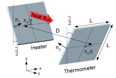
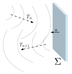
Figure 13: Left: Geometrical setup of the numerical algorithm and notations. Right: Representation of an incoming and outcoming wave at the n^th reflection.

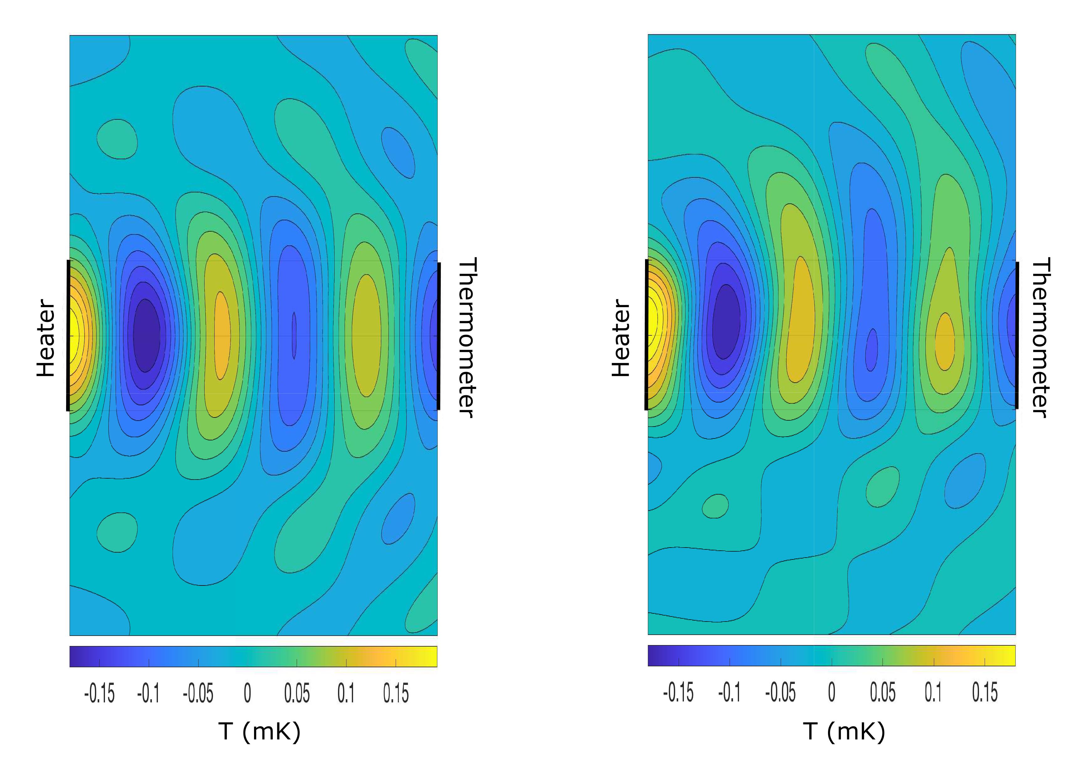
Figure 14: Left: Temperature field fluctuations of the $5^{th}$ resonant mode of second sound tweezers with aspect ratio $\frac{L}{D}=0.4$, and heating power $j_{Q}=0.185$ W/cm², at the bath temperature $T_{0}=2K$. Right: Temperature field fluctuations for the same conditions with an additional flow of velocity $\frac{U}{c_{2}}=0.18$ directed upward . The nodes of the temperature standing wave correspond to antinodes of second sound velocity, and vice-versa.

III.3.2 In the presence of a turbulent flow

One of the aims of second-sound resonator modelling is to understand their response in the present of a flow $\mathbf{U}$ sweeping the cavity. One effect of the flow is to advect the second sound wave. In the present section, we explain how the algorithm of sec. III.3.1 should be modified to account for this effect. We assume in the following that the inequality $\left|\mathbf{U}\right|<c_{2}$ is strictly satisfied, which means that the flow is not supersonic for second sound waves.

In the presence of a non-zero flow $\mathbf{U}$, the Green function (13) becomes

$$G(\mathbf{r},t)=\frac{e^{-2i\pi ft^{*}}}{\left|\mathbf{r}-\mathbf{U}t^{*}\right|\left(1+\frac{\mathbf{U}}{c_{2}}.\frac{\mathbf{r}-\mathbf{U}t^{*}}{\left|\mathbf{r}-\mathbf{U}t^{*}\right|}\right)},$$ (22)

where $t^{*}$ is the time shift corresponding to the signal propagation from the source

$$\left|\mathbf{r}-\mathbf{U}t^{*}\right|=c_{2}t^{*}.$$ (23)

In practice, the flow velocity range reached in quantum turbulence experiments is most often much lower than the second sound velocity, with $\left|\mathbf{U}\right|$ hardly reaching a few m/s. Most experiments are done in the temperature range where $10<c_{2}<20$ m/s. We thus introduce the small parameter $\mathbf{\beta}=\frac{\left|\mathbf{U}\right|}{c_{2}}\ll 1$. Similarly to the standard approximations of electromagnetism, we assume that the effect of $\beta$ is mostly concentrated in the phase shift $e^{-2i\pi ft^{*}}$ of Eq. (22). We use the approximation $\left|\mathbf{r}-\mathbf{U}t^{*}\right|\left(1+\frac{\mathbf{U}}{c_{2}}.\frac{\mathbf{r}-\mathbf{U}t^{*}}{\left|\mathbf{r}-\mathbf{U}t^{*}\right|}\right)\approx\left|\mathbf{r}\right|$, and we solve Eq. (23) to obtain $t^{*}$ to leading order in $\beta$. The Green function then becomes

$$G(\mathbf{r},t)=\frac{e^{-ik\left|\mathbf{r}\right|\Gamma\left(\mathbf{r},\mathbf{U}\right)}}{\left|\mathbf{r}\right|},$$ (24)

where as previously $k=\frac{2\pi f}{c_{2}}$ and

$$\Gamma\left(\mathbf{r},\mathbf{U}\right) =1-\frac{\mathbf{U}}{c_{2}}.\frac{\mathbf{r}}{\left|\mathbf{r}\right|}.$$

The algorithm detailed in sec. III.3.1 can be applied straightforward with the Green function Eq. (24). In particular, Eq. (20) becomes

$$\nabla\overline{T}_{n+1}(\mathbf{r}).\mathbf{n}_{2}=\frac{-1}{2\pi}\iint_{\Sigma_{1}}G\left(\mathbf{r}-\mathbf{r}_{1},\mathbf{U}\right)\left[\left(\frac{1}{\left|\mathbf{r}-\mathbf{r}_{1}\right|}+ik\right)\frac{\mathbf{r}-\mathbf{r}_{1}}{\left|\mathbf{r}-\mathbf{r}_{1}\right|}.\mathbf{n}_{2}-ik\frac{\mathbf{U}}{c_{2}}.\mathbf{n}_{2}\right]\left[\nabla\overline{T}_{n}.\mathbf{n}_{1}\right](\mathbf{r}_{1})\;{\rm d}^{2}\mathbf{r}_{1}.$$ (25)

A simulation of the temperature field at $t=0$ of the $5^{th}$ resonant mode of second sound tweezers with aspect ratio $\frac{L}{D}=0.4$, without lateral shift nor inclination, and with a flow of velocity $\frac{U}{c_{2}}=0.18$, is displayed in the right panel of Fig. 14. The effect of the flow can be clearly seen with the upward distortion of the antinodes of the wave, compared to the reference temperature profile without flow displayed in the left panel.

III.4 Quantitative predictions

We present in this section the quantitative results obtained with the algorithm of sec. III.3. The algorithm is specifically run in the configuration of second sound tweezers, but most predictions are relevant for other types of second sound resonators. We first show that the algorithm can quantitatively account for the experimental spectra. We then use it to predict the response in the presence of a flow and a bulk dissipation in the cavity. The predictions are systematically compared to experimental results for second sound tweezers. We eventually display some experimental observations that illustrate the limits of our model.

III.4.1 Spectral response of second sound resonators

Given a resonator lateral size $L$, the model of sec. III.3 has three geometrical parameters : the gap $D$, the inclination $\gamma$ and the lateral shift $X_{sh}$ (see notations in Fig. 13). We first sketch qualitatively the importance of those three parameters.

The gap $D$ is the main parameter: it sets the location of the resonant frequencies, and the quality factor of the resonances at low mode numbers. For second sound tweezers, the value of $D$ can be usually obtained within a precision of a few micrometers ($D$ is of the order of 1 millimeter). The relative inclination of the plates $\gamma$ is responsible for the saturation of the resonant magnitude and its decrease at large mode numbers. It is typically smaller than a few degrees. Contrary to the gap, only the order of magnitude of $\gamma$, not its precise value, can be determined from the tweezers’ spectrum. The lateral shift $X_{sh}$ has very little impact on the spectrum if the value $\frac{X_{sh}}{L}$ remains small enough (we can typically reach $\frac{X_{sh}}{L}<0.1$ in the tweezers’ fabrication). However, the effect of this parameter is of paramount importance to understand open cavity resonators response in a flow (such as second sound tweezers), and will be investigated in sec. III.4.2. We consider the case $X_{sh}=0$ in the present section. The tweezers size $L$ is known from the probe fabrication process.

The method goes as follows: we first find a gap rough estimation $\widetilde{D}$, for example from the average spacing between the experimental resonant peaks. Then we can run a simulation for parallel plates ($\gamma=0$), unit gap $D=1$, and aspect ratio $\frac{L}{\widetilde{D}}$, in the range $0<k^{*}<n\pi$ (where $n$ is the number of modes to be fitted, and $k^{*}=kD$ is the non-dimensional wave number). This gives a function $f_{L/\widetilde{D}}(k^{*})$. The experimental spectrum can then be fitted with the function $T(f)=Af_{L/\widetilde{D}}(\frac{2\pi fD}{c_{2}})$, where $A$ and $D$ are the two free parameters to be fitted, provided the experimental value of $c_{2}$ is known. The high sensitivity of the location of the resonant frequencies makes this method very accurate to obtain the gap $D$.

Once $D$ has been found, new simulations have to be run to find the order of magnitude of $\gamma$. As was previously said, $\gamma$ controls the saturation and the decrease of the resonant magnitudes for large mode numbers. Its value can thus be approximated from a fit of the resonant modes with the largest magnitude. A fit of an experimental tweezers spectrum is displayed in Fig. 15. The values of the fitting parameters for this spectrum are $D=1.435\pm 0.003$ mm and $\gamma=4.2\pm 0.5$ deg. Given the simplicity of the model assumptions, in particular the assumptions of perfectly insulating and infinitely thin plates without support arms, the agreement with experimental results is very good.

Interestingly, the resonators can also be used in some conditions as thermometers. Once the gap $D$ is known with high enough precision, the spectrum can be fitted using $c_{2}$ as a fitting parameter instead of $D$. Away from the second sound plateau of the curve $c_{2}(T_{0})$ located around $1.65$ K, the value of $c_{2}$ obtained from the spectrum gives access to the average temperature with a typical accuracy of one mK, simply by inverting the function $c_{2}(T_{0})$.

Figure 15: The second sound tweezers experimental spectrum of Fig. 9 (blue curve) and the result of the numerical algorithm (red curve). The remaining fitting parameters of the model are the gap $D$, the inclination $\gamma$ and the total heating power.

III.4.2 Response with a flow

Once the characteristics of the resonator have been determined in a background medium at rest, their response in a flow can be studied using the modified algorithm presented in sec. III.3.2. We experimentally observe that the tweezers response is attenuated in the presence of a superfluid helium flow. This attenuation is related to two physical mechanisms, illustrated in Fig. 16: first, the thermal wave crossing the cavity is damped by the quantum vortices carried by the flow. This type of damping is usually considered as being proportional to the density of quantum vortex lines between the plates. Secondly, the flow mean velocity is responsible for a ballistic advection of the thermal wave outside the cavity. The thermal wave emitted by the heater partly “misses” the thermometer plate, and, even if the wave is not attenuated, a decrease of the tweezers’ response will be observed. Both mechanisms described above exist in experimental superfluid flows, and cannot be observed independently: once there is a superfluid flow, quantum vortices are created. One key objective is to be able to separate the attenuation of the experimental signal due to bulk attenuation inside the cavity, from the attenuation due to ballistic advection of the wave outside the cavity. We will introduce a mathematical procedure to perform such a separation for a fluctuating signal.

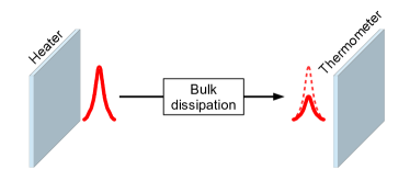
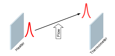
Figure 16: Schematic representation of the two attenuation mechanisms. The top panel illustrates a bulk dissipation of the wave, due for example to the presence of quantum vortices. The bottom panel illustrates the ballistic deflection of the wave by a flow directed parallel to the plates.

What cannot be experimentally achieved can be simulated with the tweezers model developed in sec. III.3. The bulk dissipation can be implemented in the algorithm with a wave number complex part $\xi$ (see Eq. (21)), and the flow ballistic deflection can be implemented with a non-zero velocity $\mathbf{U}$ (see Eqs. (24-25)). Both effects can be independently studied, by alternatively setting $\xi$ or $\mathbf{U}$ to zero. We first detail below the respective effects of $\xi$ and $\mathbf{U}$ for perfectly aligned plates ($X_{sh}=0$).

Fig. 17 display the result of a numerical simulation for second sound tweezers of aspect ratio $L/D=1$, $\gamma=0$ and increasing values of bulk dissipation in the range $0<\xi D<0.2$. The left panel display the magnitude of the second resonant mode as a function of the wave number, and the right panel display the same resonant mode in the phase-quadrature plane. More precisely, if we call $T(k)$ the thermal wave magnitude recorded by the thermometer, and $\varphi(k)$ its phase, the right panel displays the curve $Y(k)=T(k)\sin(\varphi(k)),X(k)=T(k)\cos(\varphi(k))$.

The resonant curve $(Y(k),X(k))$ is called in the following the resonant “Kennelly circle” (see also sec. IV.2), because the curve is very close to a circle crossing the origin. Furthermore, the resonant curve becomes closer to a perfect circle for increasing resonant quality factors. The major characteristic to be observed in Fig. 17 is that the collapse of the resonant Kennelly circle due to bulk attenuation is homothetic. It means that the different curves have no relative phase shift between each other, when the bulk attenuation increases. The red curves in the right panel display the displacement in the phase-quadrature plane for a fixed value of the wavevector. The model predicts that the displacement is directed toward the Kennelly circle center, which implies that the path at a fixed wavevector approximately follows a straight line. By comparison, the left panel of Fig. 19 display an experimental resonance in the phase-quadrature plane, for second sound tweezers of size $L=1$ mm in superfluid Helium at $1.65$ K. The global orientation of the resonant Kennelly circles is simply due to a uniform phase shift introduced by the measurement devices, and should be overlooked. It can be seen that the resonance collapse with increasing values of the flow velocity follows the predictions of Fig. 17: it is homothetic. The red paths correspond to the tweezers signal at fixed heating frequency. Those paths follow approximately a straight line directed to the Kennelly circle center. The slight deviation in the path orientation from the predictions of Fig. 17 can be explained by a second sound velocity reduction and will be discussed in sec. III.4.4.

Fig. 18 display the result of a numerical simulation for second sound tweezers of aspect ratio $L/D=1$, $\gamma=0$, with $\xi=0$ and a flow mean velocity $0<\frac{U}{c_{2}}<0.2$. As there is no tweezers lateral shift $X_{sh}=0$, negative velocities would lead to the same result from symmetry considerations. The figure illustrates the effect of pure ballistic advection on a resonance in the phase-quadrature plane. First, it can be seen that the collapse of the resonant Kennelly circle is accompanied by a relative anti-clockwise phase shift of the curves when the velocity increases. Also, the displacement of the tweezers signal at fixed wavenumber follow the red straight paths directed anti-clockwise. This type of signal strongly contrasts with the one of Fig. 17 obtained for a pure bulk attenuation. The prediction of the left panel in Fig. 18 cannot be directly compared to experiments because, as stated before, a superfluid flow always carries quantum vortices that overwhelm the tweezers signal for tweezers satisfying $X_{sh}\approx 0$.

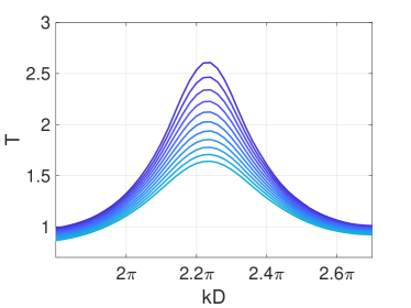
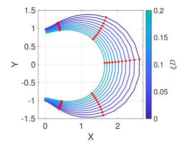
Figure 17: Numerical simulation: collapse of a resonance due to increasing values of the bulk attenuation $\xi$. The left panel display the magnitude of the thermal wave as a function of the wavevector $k$, and the right panel display the same resonance in the phase-quadrature plane. It can be seen that the bulk attenuation results in a homothetic collapse of the resonance, that means, without global phase shift. For a given value of $k$, the model predicts that attenuation is directed toward the center of the resonant Kennelly circle (red curves of right panel).

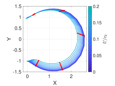
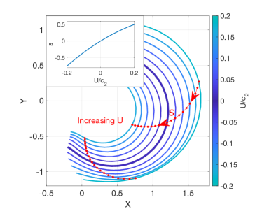
Figure 18: Numerical simulation: collapse of a resonance due to ballistic deflection of the thermal wave in the presence of a flow of velocity $U$, without bulk attenuation ($\xi$=0). The left panel display the result for tweezers without lateral shift ($X_{sh}=0$). Contrary to the results of Fig. 17, it can be seen in the present case that the collapse is associated with a global anti-clockwise phase shift of the resonant Kennelly circle. Each red curve represents the attenuation at a given value of the wavevector $k$. The right panel displays the result for tweezers with a strong lateral shift $X_{sh}=0.5\times L$ (where L is the tweezers size). Such tweezers are very sensitive to the velocity $U$, with both an attenuation of the resonance and a strong clockwise angular shift of the Kennelly circle. We note $s$ the curvilinear abscissa of the curve obtained at a given value of $k$ (red curve). The inset displays the function $s(U)$. This shows that, once calibrated, second-sound tweezers can be used as anemometers.

III.4.3 Effect of lateral shift of the emitter and receiver plates

We discuss in this section the consequences of a lateral shift, that is $X_{sh}\neq 0$ with the notations of Fig. 13. Contrary to the previous sections, the present discussion is restricted to second sound tweezers, for which a lateral shift has major quantitative effects. A lateral shift would not be as important, for example in the case of wall embedded resonators.

The lateral shift has a marginal effect on the tweezers’ spectrum when the background fluid is at rest. An effect only appears in the presence of a nonzero velocity specifically oriented in the shifting direction $\mathbf{U}=U\mathbf{e}_{x}$, because of the mechanism of ballistic advection of the thermal wave by the flow (see the representation of the mechanism in Fig. 16). The importance of this effect depends on the tweezers’ aspect ratio, on the reduced velocity $\beta=\frac{U}{c_{2}}$, and on the lateral shift $X_{sh}$. The lateral shift in the plates’ positioning magnifies the signal component related to ballistic advection. This property opens the opportunity to build second sound tweezers for which ballistic advection of the wave completely overwhelms bulk attenuation from the quantum vortices, which means that the tweezers signal is in fact a measure of the velocity component in the shifting direction. We illustrate this mechanism in Fig. 18.

The right panel displays a numerical simulation of a tweezers resonant mode in the phase-quadrature plane, for the parameters $\frac{L}{D}=1$, $\gamma=0$ and $X_{sh}=0.5$, for positive and negative values of the flow velocity in the range $-0.2<\frac{U}{c_{2}}<0.2$. As can be seen at the first sight, the deformation of the resonant curve - that we equivalently call the Kennelly circle - is very different from a deformation due to a bulk attenuation (see Fig. 17). First, we observe that the deformation can result in an increase of the magnitude of the thermometer signal, when the velocity is negative. This can be explained in this configuration, because the thermal wave emitted by the heating plate is redirected toward the thermometer plate: less energy is scattered outside the cavity when the wave is first emitted by the heater, and the signal magnitude increases. On contrary, the signal magnitude decreases when the velocity is positive because the flow advects the emitted thermal wave further away from the thermometer plate and more energy is scattered outside the cavity. Second, the deformation of the Kennelly circle is associated to a global clockwise rotation, a phenomenon that is not observed for bulk attenuation in Fig. 17. Coming back to Fig. 18, the red curve displays the displacement in the phase-quadrature plane for a fixed wave frequency value. The displacement follows a very characteristic curved path, always directed clockwise. Let $s(U)$ be the curvilinear abscissa of the red path. Once calibrated, the value of $s$ can be used as a measure of the flow velocity component in the $\mathbf{e}_{x}$ direction.

The right panel of Fig. 19 displays the experimental signal observed with second sound tweezers of size $L=250$ $\mu{\rm m}$, $D=431$ $\mu{\rm m}$ and $X_{sh}\approx 125$ $\mu{\rm m}$, for a positive velocity range $0<U<1$ m/s. The main characteristics of a ballistic advection signal can be observed: the Kennelly circle are attenuated with a clear clockwise rotation, and the signal at fixed frequency follows a curved path in the clockwise direction. This is a strong indication that those type of tweezers can be used as anemometers. The signal fluctuations of those type of tweezers were recently characterized in a turbulent flow of superfluid helium WVR (21). It has been shown in particular that both the signal spectra and its probability distributions indeed display all the characteristics of that of turbulent velocity fluctuations.

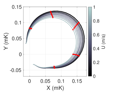
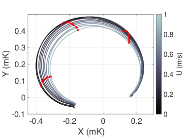
Figure 19: Experiment: Collapse of a second sound resonance for increasing values of the flow mean velocity $U$, in superfluid Helium at $T_{0}\approx 1.65$ K. The right panel display the result for tweezers of size $L=1$ mm and minor lateral shift $X_{sh}<0.1\times L$. The figure shows a homothetic collapse of the resonant Kennelly circle without global phase shift, as predicted by the model of Fig. 17. The red curves display the displacement in the phase-quadrature plane at a fixed value of the second sound frequency $f$. The right panel displays the experimental data obtained with shifted second sound tweezers with parameters $L=250$ $\mu{\rm m}$ and $X_{sh}=0.5\times L$. The figure qualitatively confirms the clockwise angular shift with increasing values of $U$, predicted by the numerical simulations of Fig. 18.

III.4.4 Limits of the model

Although the model of sec. III.3 gives excellent experimental predictions, we still observe some unexpected phenomena with real second sound tweezers. We discuss two of them in this section.

We have seen in secs. III.4.2 that the thermal wave complex amplitude $\overline{T}(f)$ can be represented in the phase-quadrature plane by a curve $(X(f),Y(f))$ very close to a circle crossing the origin. This osculating circle will be called hereafter the resonant “Kennelly circle” (a more precise definition is given in sec. IV.2). The wave is damped in the presence of a superfluid flow, which can be seen in the phase-quadrature plane as a homothetic shrink of the Kennelly circle toward the origin. Fig. 20 displays an experimental resonance in the phase-quadrature plane, for $U=0$ m/s and $U=0.7$ m/s, together with the fitted Kennelly circles. As can be seen in the figure, the resonant curve at $U=0$ has periodic oscillations in and out of the Kennelly circle. We call this phenomenon the “daisy effect”. The daisy effect progressively disappears for increasing values of $U$, and cannot be seen any more on the resonant curve at $U=0.7$ m/s. We interpret the daisy effect as a secondary resonance in the experimental setup with a typical acoustic path of a few centimeters. We assume that the flow kicks out the thermal wave from this secondary resonant path when $U$ is increased. The daisy effect alters the attenuation measurements close to $U=0$, and should be considered with care before assessing the vortex line densities for very low mean velocities.

It has been shown in sec. III.4.2 that the displacement of the tweezers signal in the phase quadrature plane, for a fixed wave frequency, follows a straight line. We call “attenuation axis” the direction of this straight path. The model predicts that the attenuation axis should always be directed toward the center of the resonant Kennelly circle. Fig. 21 displays a zoom on a part of the Kennelly circle at $U=0$, together with the signal displacement at fixed frequency and for increasing flow velocity. It can be seen that the displacement is indeed a straight line, but not exactly directed toward the Kennelly circle center. An angle between $20^{\circ}$ and $30^{\circ}$ is systematically observed between the attenuation axis and the circle center direction (see Fig. 21). Moreover, the angle is always positive (with the figure convention) and cannot be interpreted as a ballistic advection, that would give a negative angle instead. This effect is thus very likely been attributed to a decrease of the second sound velocity in the presence of the quantum vortices. Whereas a second sound velocity reduction has previously been observed in the presence of quantum vortices LV (74); Meh (74); MLM (78), the exact value of this reduction turns to be difficult to assess in particular experimental conditions. We therefore keep the second sound velocity reduction as a qualitative explanation, and we do not try to assess quantitative result from the attenuation axis angle.

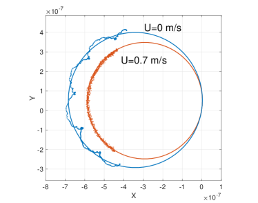
Figure 20: Experimental resonance obtained with a second sound tweezers at 1.98 K, for two values of the He flow mean velocity $U$. The blue curve displays a periodic perturbation of the resonance that we refer to as the “daisy effect”. The circle is a fit of the Kennelly osculating circle for this resonance. This effect is not predicted by our model, and we interpret it as a secondary resonance in the experimental setup. The daisy effect perturbs the measurements at low values of $U$, but it can be seen on the red curve that the effect disappears for higher values of $U$.

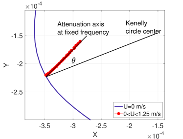
Figure 21: Attenuation of a resonance in the presence of a flow mean velocity $U$, obtained with second sound tweezers in superfluid Helium at 1.65 K. The blue curve is the resonance at $U=0$ in the phase-quadrature plane. Contrary to the prediction of the model of section III.4 (see also Fig. 17), the attenuation signal at fixed heating frequency is not directed exactly toward the centre of the Kennelly osculating circle. We observe a systematic clockwise angular shift $20{{}^{\circ}}<\theta<30{{}^{\circ}}$. We still have no definite explanation for this observation.

III.5 Quantum vortex or velocity measurements ?

We have shown that second sound resonators are sensitive to two physical mechanisms. The first one is the thermal wave bulk attenuation inside the tweezers’ cavity, due to the quantum vortices. The second one is thermal wave ballistic advection perpendicular to the plates. Both mechanisms exist for all the second sound resonators, but depending on their geometry, they can preferentially be sensitive to the one or the other mechanism. We call selectivity the fraction of the signal due to quantum vortices or to ballistic advection. Let $\overline{T}\left(\xi,U\right)$ be the probe signal as a function of the bulk attenuation coefficient $\xi$ (m^-1) and flow velocity $U$(m/s), we define the vortex selectivity as

$$\mathcal{R}_{\xi}=\frac{\left|\overline{T}\left(\xi,0\right)-\overline{T}\left(0,0\right)\right|}{\left|\overline{T}\left(\xi,U\right)-\overline{T}\left(0,0\right)\right|}.$$ (26)

and by symmetry we define the velocity selectivity as

$$\mathcal{R}_{U}=\frac{\left|\overline{T}\left(0,U\right)-\overline{T}\left(0,0\right)\right|}{\left|\overline{T}\left(\xi,U\right)-\overline{T}\left(0,0\right)\right|}.$$ (27)

Further investigations in second sound tweezers experiments have shown that the velocity/vortex selectivity process only weakly depends on the aspect ratio $\frac{L}{D}$. Indeed, for a given resonator lateral size $L$, ballistic advection of the wave outside the cavity increases when the gap $D$ increases, but the number of quantum vortex lines inside the cavity also increases linearly with $D$. Altogether, both the ballistic advection and the bulk attenuation due to the quantum vortices have similar dependence with $D$, that’s why changing the gap has no significant effect on selectivity. For second sound tweezers, we observe that the selectivity neither depends strongly on the mean temperature (that controls the superfluid fraction and the second sound velocity).

As explained in sec. III.4.2, the velocity selectivity is more important for open cavity resonators such as second sound tweezers. For a given tweezers size, we find that the selectivity depends mainly on the shift $X_{sh}$ and on the wave mode number. Perfectly aligned tweezers excited with low mode numbers are preferentially sensitive to quantum vortices. Increasing $X_{sh}$ or choosing larger mode numbers leads to a larger velocity sensitivity and changes the signal balance from vortex selectivity to velocity selectivity. The tweezers’ selectivity also strongly depends on the size $L$: smaller tweezers can encompass less quantum vortices in the cavity, which means that the total wave attenuation from one plate to the other is smaller for small tweezers. By contrast, the attenuation fraction due to velocity advection does not depend on the tweezers size. The velocity selectivity is thus larger when the tweezers are smaller. Fig. 22 displays the selectivity of two second sound tweezers of size $L=250$ $\mu{\rm m}$ and $L=1$ mm respectively, depending on the shift $X_{sh}$ and the mode number $n$ (where $k=n\pi$). The simulation was run with a quantum vortex line density $\mathcal{L}=2\times 10^{10}$ m^-2 and $U=1$ m/s, in accordance with the typical values observed in the experiments of WVR, 21. It can be seen that large tweezers ($L=1$ mm) can reach a vortex selectivity $\mathcal{R}_{\xi}>90\%$ for a small shift and low mode number, which means that they can be used for direct quantum vortex measurements. On contrary, small tweezers ($L=250$ $\mu{\rm m}$) can reach a velocity selectivity $\mathcal{R}_{U}>90\%$ for large shift or high mode number, and can thus be used as anemometers, as confirmed by the experiments reported in WVR, 21.

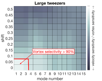
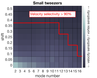
Figure 22: Selectivity to quantum vortices or velocity advection for two second sound tweezers, obtained with numerical simulations. The color code indicates the fraction of the signal due to bulk attenuation by quantum vortices (see Fig. 16). The selectivity of the tweezers mainly depends on the lateral shift of both plates one from another, and the resonant mode number excited in the cavity. The left panel shows that large tweezers ($L=1$mm) are mainly sensitive to quantum vortices. Almost pure quantum vortex signal can be achieved with carefully aligned tweezers excited at low mode numbers ($\mathcal{R}_{\xi}>90\%$). On the reverse, small tweezers ($L=250\mu{\rm m}$) are mainly sensitive to the velocity. Almost pure velocity signal can be achieved by shifting the heater and the thermometer plates and by exciting the cavity at large mode numbers ($\mathcal{R}_{U}>90\%$). The present simulation was run with a vortex line density $\mathcal{L}=2\times 10^{10}$ m^-2 and $U=1$ m/s, in accordance with the typical values observed in our experiments.

IV Measurements with second sound tweezers

Second sound tweezers are singular sensors in the sense that they can measure two degrees of freedom at the same time, whereas most of hydrodynamics sensors only measure one (e.g. Pitot tubes, cantilevers, hot wires). The tweezers record the magnitude and phase of the thermal wave averaged over the thermometer plate. Both quantities contain physical information about the system. To summarize it shortly, magnitude variations give information about quantum vortices in the cavity, whereas phase variations give information about the local mean temperature and pressure. The local mean velocity has an impact on both magnitude and phase, and will be specifically treated in sec. IV.5. The aim of the following sections is to explain how properly separate quantum vortices signal from other signal components.

In the following, we call $\mathcal{L}_{\perp}$ the density of projected quantum vortex lines density (projected VLD)

$$\mathcal{L}_{\perp}=\frac{1}{\mathcal{V}}\int_{\mathcal{V}}\sin^{2}\theta(l){\rm d}l,$$ (28)

where $\mathcal{V}$ is the tweezers’ cavity volume, $l$ is the curvilinear abscissa along the vortex lines inside the cavity , $\theta(l)$ is the angle between the quantum vortex line and the direction perpendicular to the plates (vector $\mathbf{e}_{z}$). Assuming isotropy of the vortex tangle, the total quantum vortex lines density (VLD) is

$$\mathcal{L}=\frac{3}{2}\mathcal{L}_{\perp}.$$ (29)

A second sound wave is damped in the presence of a tangle of quantum vortices. Let $\xi_{VLD}$ (in m^-1) be the bulk attenuation coefficient of second sound waves, it has been foundHV56a ; HV56b ; Tsa (62); SP (66); MPS (84) that $\xi_{VLD}$ is proportional to $\mathcal{L}_{\perp}$ according to the relation

$$\xi_{VLD}=\frac{B\kappa\mathcal{L}_{\perp}}{4c_{2}},$$ (30)

where $B$ is the first Vinen coefficient and $\kappa\approx 9.98\times 10^{-8}$ m²/s (for ⁴He) is the quantum of circulation around one vortex.

Therefore, Eq. (30) shows that a measure of the bulk attenuation coefficient gives access to the projected VLD defined by Eq. (28). We recall in sec. IV.1 the standard methods to measure the bulk attenuation coefficient from a second sound resonance, and we propose in sec. IV.3 two new analytical methods and we give in sec. IV.4 some examples to apply our elliptic method to the experimental data.

IV.1 The vortex line density from the attenuation coefficient

We assume that a single second sound resonance can be accurately represented by the following expression (see Eq. (11))

$$\overline{T}(f)=\overline{T}_{0}\frac{\sinh\left(\xi_{0}D\right)}{\sinh\left(i\frac{2\pi(f-f_{0})D}{c_{2}}+(\xi_{0}+\xi_{VLD})D\right)},$$ (31)

where $f_{0}$ is the second sound frequency of the local amplitude maximum, $D$ is the resonator gap, $c_{2}$ is the second sound velocity, $\xi_{0}$ is the attenuation coefficient without flow and $\xi_{VLD}$ is the additional bulk attenuation in the presence of quantum vortices given by Eq. (30). $\xi_{VLD}=0$ without flow.

A standard method to measure $\xi_{VLD}$ goes as follows: we fix the second sound frequency at the resonant value $f_{0}$, and we measure the thermal wave amplitude with, and without flow. Eq. (31) then shows that $\xi_{VLD}$ is given by

$$\xi_{VLD}=\frac{1}{D}\mathrm{asinh}\left(\frac{\overline{T}_{0}}{\overline{T}(f_{0})}\sinh\left(\xi_{0}D\right)\right)-\xi_{0}.$$ (32)

Eq. (32) shows that beside the value of $D$, that can be determined from a fit of the tweezers’ spectrum (sec. III.4), the value of $\xi_{0}$ has to be accurately measured. This is usually done by the measurement of the resonant half width. With some algebra manipulations, it can be found from Eq. (31) that the resonant magnitude satisfies

$$\left|\overline{T}\right|^{2}=\left|\overline{T}_{0}\right|^{2}\frac{\sinh^{2}\left(\xi_{0}D\right)}{\sinh^{2}\left(\xi_{0}D\right)+\sin^{2}\left(\frac{2\pi(f-f_{0})D}{c_{2}}\right)}.$$ (33)

Let $\Delta f$ be the frequency half-width defined by the relation $\left|\overline{T}(f_{0}\pm\frac{\Delta f}{2})\right|^{2}=\frac{1}{2}\left|\overline{T}_{0}\right|^{2}$, it can be shown from Eq. (33) that $\xi_{0}$ and $\Delta f$ are related by

$$\sin\left(\frac{\pi\Delta fD}{c_{2}}\right)=\sinh\left(\xi_{0}D\right).$$ (34)

We note in particular that the relation (34) can be used to find $\xi_{0}$ as long as the resonance quality factor is high enough, that means, for $\sinh\left(\xi_{0}D\right)<1$. The linear approximations of Eqs. (32) and (34) are usually used when $\xi_{0}D\ll 1$, and they give the well-known approximation:

$$\mathcal{L}_{\perp}\simeq\frac{4\pi\Delta f}{B\kappa}\left(\frac{\overline{T}_{0}}{\overline{T}(f_{0})}-1\right),$$ (35)

For low quality factor resonances, another method should be used instead of the resonant half width. The elliptic method presented in sec. IV.3 allows determining $\xi_{0}$ for resonances of any quality factors.

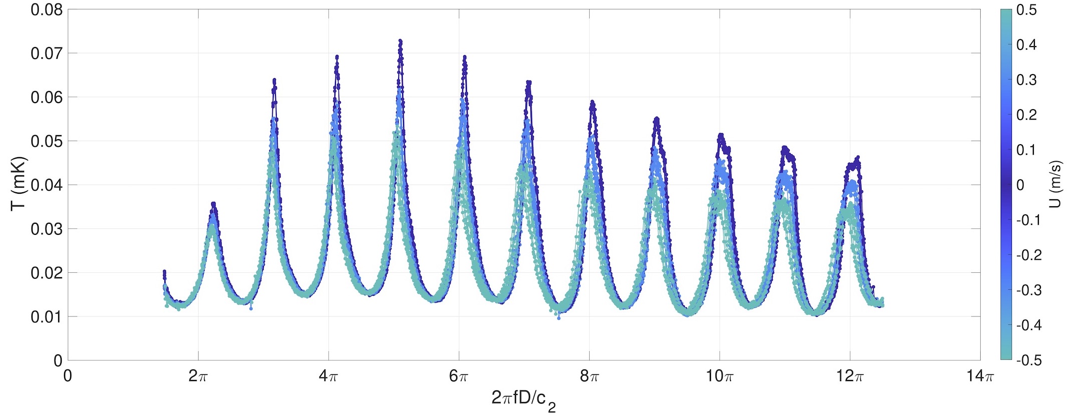
Figure 23: Spectral response of tweezers in a turbulent boundary layer of the SHREK facility, right below the superfluid transition temperature $T_{\lambda}$, where second sound velocity $c_{2}$ is very sensitive to temperature (here $D\simeq 500\>\mu$m and $c_{2}$ drifts around a mean value of $5.4\>m/s$). The frequency axis is adimensionalize using the second sound velocity $c_{2}$ calculated from the temperature recorded near the sidewall of the flow. While the temperature of the bath is regulated, frequency sweeps are repeated half a dozen of times for different turbulent flow conditions flagged by colors. A systematic drift of resonance frequencies versus flow conditions is observed ; it is interpreted as an under-estimation of temperature, and therefore over-estimate of $c_{2}$, due to turbulent dissipation in the core of the flow. At a given mean flow, some scatter of the resonance frequencies is apparent ; it is interpreted as noise from the temperature regulation. The elliptic method introduced in section IV.3 allows separating such temperature artifacts from the attenuation due to second sound attenuation by quantum vortices.

The main problem of the method presented above is that it implicitly assumes that there is no variation of the acoustic path value $\frac{2\pi f_{0}D}{c_{2}}$ during the measurement. In particular, as $c_{2}$ depends on temperature and pressure, it means that the experiment should have an excellent temperature and pressure regulation. This can become increasingly difficult when the second sound derivatives versus temperature become steep, close to the superfluid transition. Moreover, measurements in the presence of a flow are necessary done out of equilibrium as the flow dissipates energy. As an example, measurements in such conditions are illustrated by figure 23, which shows second sound resonances measured close to the superfluid transition in the turbulent Von Kármán experiment SHREK RBD⁺ (14). Furthermore, we observe that a measurement with a non-zero value of $\xi_{VLD}$ can be associated with an acoustic path shift (i.e. a variation of the factor $\frac{2\pi fD}{c_{2}}$). The situation is illustrated in the left panel of Fig. 24, where the acoustic path shift leads to an overestimation of the attenuation and an important error on $\xi_{VLD}$.

Passive and active approaches have been reported in the literature to handle the most common cause of acoustical path shift during second sound measurement: the temperature drift and its resulting shift of the resonance frequency.

A passive approach consists in performing a sweep of the second sound frequency, across the resonance curve. Afterward, with proper modelling of the resonance, the attenuation and the phase shift can be fitted separately, e.g. as done in MSS, 76. A limit of this approach is its time resolution, that is restricted by the duration of frequency scan. Another passive approach consists in performing systematic calibration of the full frequency responses of the resonator in various conditions, and subsequently interpolating measurements obtained at a fixed working frequency onto this mapping VBL⁺ (17).

A standard example of active approaches consist in controlling the helium bath temperature. An alternative or complementary approach consists in controlling the second-sound frequency so that it always matches the resonance peak, despite possible drift of the temperature. The resonator itself can provide the feedback signal of these control loops, for example by monitoring the thermometer or locking the phase of the second sound signal. An even more direct approach has been recently proposed: the resonator is driven by a self-oscillating circuit, which frequency adapts dynamically to the drift of the second sound velocity YIE (17).

Below, we introduce two analytical methods to separate phase shift from attenuation. The first method is relevant for simple cases (sec. IV.2), while the second one has a broader range of validity (sec. IV.3).

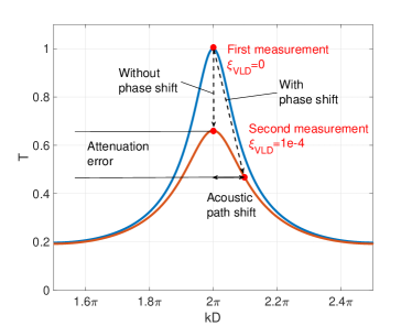
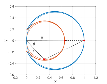
Figure 24: An illustration of an attenuation measurement. Left: the resonant mode without (blue curve), and with quantum vortex attenuation (red curve). The figure shows that an acoustic path shift can lead to an important error in the attenuation measurement. The wave vector is given by $k=\frac{2\pi f}{c_{2}}$. Right: the resonant mode represented in the phase-quadrature plane, together with the fitted Kennelly circle (defined later in sec. IV.2). The figure shows that the acoustic path shift creates a phase shift $\theta$. Using the phase measurement $\theta$, the maximal magnitude can be recovered using Eq. (IV.2).

IV.2 Analytical method in an idealized case

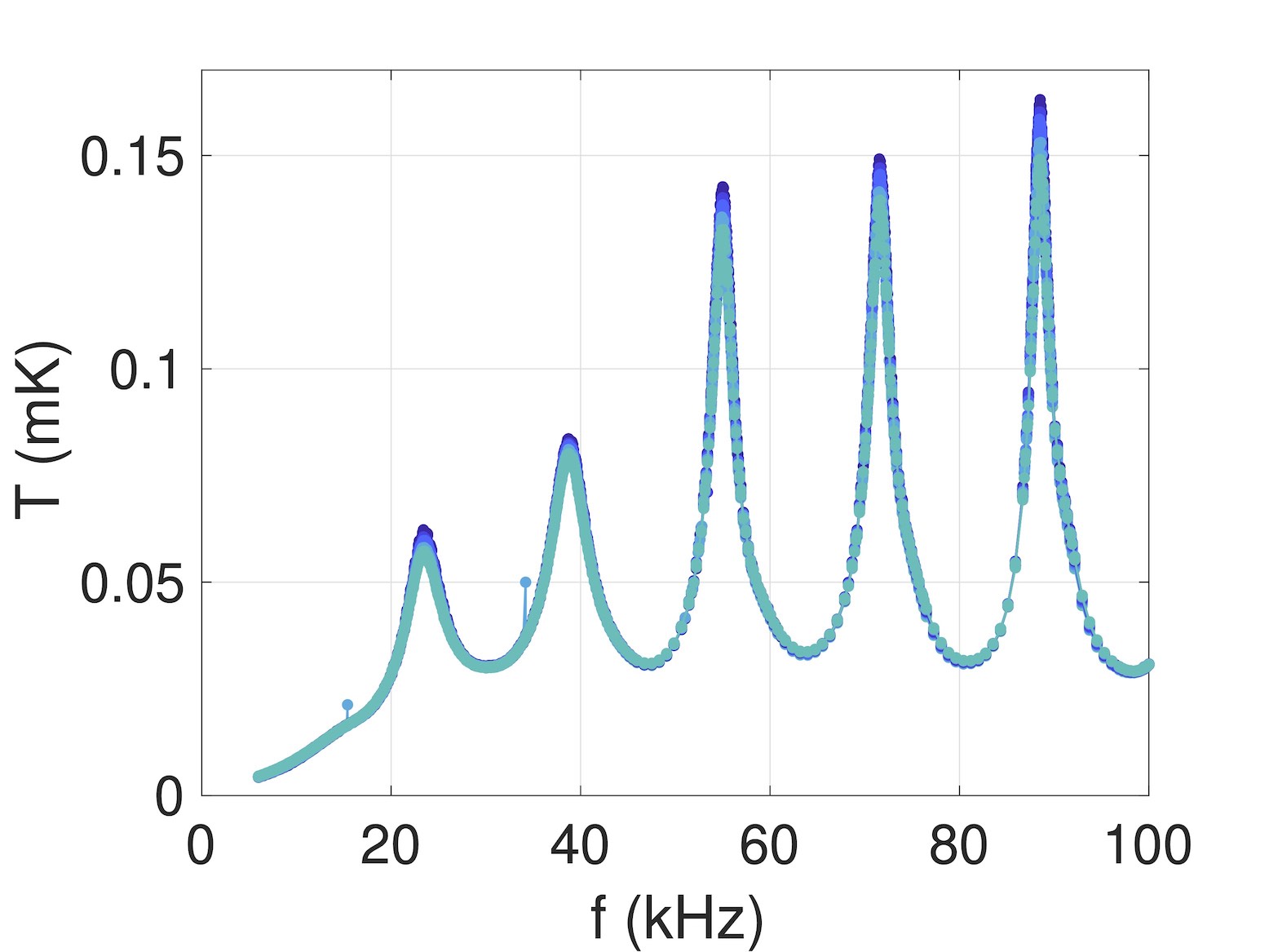
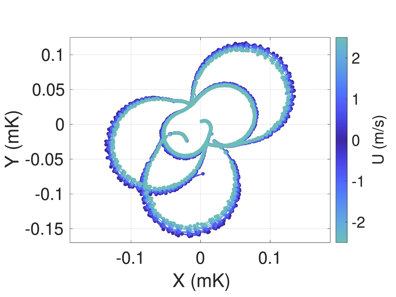
Figure 25: Sequence of five resonances of second sound tweezers at 1.6K. The flow is weakly turbulent: the velocity standard deviation is a few percents of the mean velocity displayed on the color bar. The right side plot illustrates that each resonance can be approximated by a circle in the complex plane. The global phase shift of the last resonance (lower circle) compared to the others is attributed to a cut-off of the measurement electronics at high frequency.

The acoustic path shift can be corrected using the resonant representation in the phase-quadrature plane. Let $X(f)$ and $Y(f)$ be respectively the real and imaginary parts of $\overline{T}(f)$, the curve $(X(f),Y(f))$ in the phase-quadrature plane is very close to a circle crossing the origin. It can even be proved (see sec. IV.3) that the resonant curve converges to a circle when the quality factor increases, or equivalently when $\xi_{0}$ decreases. An illustration of two resonant curves with their osculating circles is displayed in the right panel of Fig. 24. The acoustic path shift translates in a phase shift $\theta$ in the phase-quadrature plane, such that the amplitude of the second measurement (with $\xi_{VLD}>0$) does not correspond to the maximal amplitude $R$ of the attenuated resonant peak (see Fig. 24 for the notations). Using the geometric properties of the (Kennelly) circle, $R$ can be approximately recovered from the measured amplitude $r$ and phase slip $\theta$ with

$$R=\frac{r}{\cos\theta}.$$

Thus, a modified version of Eq. (32) can be written to find the VLD attenuation coefficient in the presence of a phase shift

$$\xi_{VLD}=\frac{1}{D}\mathrm{asinh}\left(\frac{\overline{T}_{0}\cos\theta}{\overline{T}(f_{0})e^{-i\theta}}\sinh\left(\xi_{0}D\right)\right)-\xi_{0}.$$ (37)

Using this equation, Eq. 30 and and Eq. 34, the VLD $\mathcal{L}$ can then be derived.

IV.3 The elliptic method

We present in this section an original method to obtain the values of the acoustic path shift and the attenuation coefficient, from experimental data. The method, that we call the “elliptic method”, is much simpler to implement, and much more reliable, than the fit of the Kennelly resonant circle and the use of Eq. (37). Besides, the method can be used for resonances with very low quality factors.

The method comes from the observation that a pair of two ideal consecutive resonances is transformed into an ellipse with the complex inversion $z\rightarrow\frac{1}{z}$ in the phase-quadrature plane. The inversion is represented in Fig. 26. To prove this assertion, consider the inversion of the classical Fabry–Perot expression Eq. (6)

$$\frac{1}{\overline{T}}=\frac{\sinh\left(i\frac{2\pi fD}{c_{2}}+\xi D\right)}{A}.$$ (38)

Expanding the $\sinh$ in the previous expression gives

$$\frac{1}{\overline{T}}=\cos\left(\frac{2\pi fD}{c_{2}}\right)\frac{\sinh\left(\xi D\right)}{A}+i\sin\left(\frac{2\pi fD}{c_{2}}\right)\frac{\cosh\left(\xi D\right)}{A}.$$ (39)

Finally, let $X_{l}=\mathcal{R}e\left(\frac{1}{\overline{T}}\right)$ and $Y_{l}=\mathcal{I}m\left(\frac{1}{\overline{T}}\right)$ be respectively the real and imaginary parts of Eq. (39), the coordinates $(X_{l},Y_{l})$ satisfy the equation

$$\left(\frac{X_{l}}{\sinh\left(\xi D\right)/A}\right)^{2}+\left(\frac{Y_{l}}{\cosh\left(\xi D\right)/A}\right)^{2}=1$$ (40)

which is exactly the Cartesian equation of an ellipse with semi-major axis $a=\frac{\cosh\left(\xi D\right)}{A},$ and semi-minor axis $b=\frac{\sinh\left(\xi D\right)}{A}.$ In particular, we note that the attenuation coefficient $\xi$ can be recovered from the ratio of the semi-major and semi-minor elliptic axes using the formula

$$\xi=\frac{1}{D}{\rm atanh}\left(\frac{b}{a}\right).$$

When the quality factor increases (equivalently when $\xi$ decreases) the ellipse is flattened. The limit of infinite quality factor ($\xi\rightarrow 0$) corresponds to two parallel straight lines in the complex plane.

Second sound tweezers resonances are not ideal Fabry–Perot resonances. Yet, we have argued in sec. III.2 that a single second sound resonance can be locally fitted by the following Fabry–Perot equation (see also Eq. (11))

$$\overline{T}=\frac{A}{\sinh\left(i\frac{2\pi(f-f_{0})D}{c_{2}}+(\xi_{0}+\xi_{VLD})D\right)}.$$ (41)

This in particular means that the resonant curve in the vicinity of its maximal amplitude is transformed into a part of an ellipse with the complex inversion $z\rightarrow\frac{1}{z}$. The curve $\left(X_{l}(f),Y_{l}(f)\right)$ is very close to a straight line, for frequencies $f$ close to the resonant frequency $f_{0}$. The situation is illustrated in Fig. 27. The figure shows a part of ideal Fabry–Perot resonances given by Eq. (41), in the range $1.95\pi<kD<2.05\pi$ (where $k=\frac{2\pi f}{c_{2}}$), and for increasing values of the VLD attenuation coefficient $\xi_{VLD}$. The left panel displays the different resonant curves close to their maximal amplitudes, in the phase-quadrature plane. Using the complex inversion, those curves become almost parallel straight lines, as can be seen in the right panel. The transformation of the resonant Kennelly circles into parallel straight lines has very nice applications that we explain in the following.

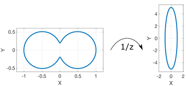
Figure 26: Transformation of a pair of consecutive resonances to an ellipse using the inversion of the complex plane $z\rightarrow 1/z$.

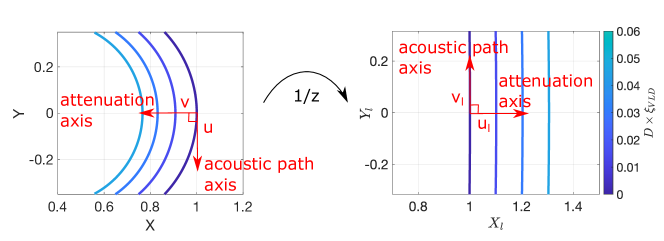
Figure 27: A resonant mode in the phase-quadrature plane and its elliptic transform, for an ideal Fabry–Perot resonance with $\xi_{0}=0.2$ and $1.95\pi<kD<2.05\pi$.

In the phase-quadrature plane, a variation of the acoustic path value $\frac{2\pi fD}{c_{2}}$ corresponds to a displacement along the Kennelly circle, whereas a variation of the bulk attenuation $\xi$ corresponds to a displacement orthogonal to the Kennelly circle. The acoustic path direction and the attenuation direction thus form a local orthogonal basis. Such a basis is displayed by the red arrows in the left panel of Fig. 27. When the reference point where the basis is defined moves along the Kennelly circle, the basis rotates and the acoustic path and attenuation axes have to be redefined. This can become a tiresome task while analyzing the experimental data. Fortunately, the complex inversion is a conformal mapping, which means that it preserves locally the angles: the local basis composed of the acoustic path and attenuation axes is transformed into an orthogonal basis (see the red arrows in the right panel of Fig. 27). More precisely, let $z_{0}$ be the complex position in the phase-quadrature plane, and $(\mathbf{u},\mathbf{v})$ be the two complex (unit) vectors defining the local basis at $z_{0}$, then the local basis $(\mathbf{u}_{l},\mathbf{v}_{l})$ at the point $\frac{1}{z_{0}}$ is given by

$$\begin{cases}\mathbf{u}_{l}&=-\mathbf{u}\frac{\left|z_{0}\right|^{2}}{z_{0}^{2}}\\ \mathbf{v}_{l}&=-\mathbf{v}\frac{\left|z_{0}\right|^{2}}{z_{0}^{2}}\end{cases}.$$ (42)

The major advantage of defining the local basis $(\mathbf{u}_{l},\mathbf{v}_{l})$ with the elliptic transform, is that it becomes a global basis: when the reference point $\frac{1}{z_{0}}$ moves because of a change in the acoustic path value or the attenuation value, the basis is simply translated in the plane, but the vectors $(\mathbf{u}_{l},\mathbf{v}_{l})$ do not change. One can find the global basis $(\mathbf{u}_{l},\mathbf{v}_{l})$ for a given resonance and use it to find the local basis $(\mathbf{u},\mathbf{v})$ at every point in the phase-quadrature plane. We will see in sec. IV.4.1 how the global basis $(\mathbf{u}_{l},\mathbf{v}_{l})$ can be easily used to suppress temperature and pressure drifts during second sound attenuation measurements.

We finally explain how the elliptic method can be used to measure the bulk attenuation coefficient $\xi_{0}$. We have seen in sec. IV.1 that the standard methods to find $\xi_{0}$ are based on the measure of the half-width $\Delta f$ and on Eq. (34). As was said previously, the classical method can only be applied to resonances satisfying $(\xi_{0}D)<1$. It is a global method, in the sense that one has to sweep the frequency to measure a large part of the resonant curve. The method is only accurate provided the resonance does not deviate too much from an ideal Fabry–Perot resonance, which is often not satisfied for the first modes of second sound tweezers (see for example the first mode of Fig. 15). The alternative method consists in expanding $(X_{l},Y_{l})$ given by Eq. (40) to leading order in $f-f_{0}$

$$\begin{cases}X_{l}&\sim\frac{\sinh\left(\xi_{0}D\right)}{A},\\ Y_{l}&\sim\frac{2\pi(f-f_{0})D}{c_{2}}\frac{\cosh\left(\xi_{0}D\right)}{A},\end{cases}$$ (43)

where $f_{0}$ is the resonant frequency. Using Eq. (43), we get

$$\frac{Y_{l}(f)}{X_{l}(f)}\sim\frac{2\pi D}{\tanh\left(\xi_{0}D\right)c_{2}}(f-f_{0}).$$ (44)

$\frac{Y_{l}(f)}{X_{l}(f)}$ is proportional to $f$ in the vicinity of $f_{0}$, with the proportionality factor $\frac{2\pi D}{\tanh\left(\xi_{0}D\right)c_{2}}$. The attenuation coefficient $\xi_{0}$ can be found by a linear fit of the function $\frac{Y_{l}}{X_{l}}$ provided $D$ and $c_{2}$ are known.

IV.4 Applications of the elliptic method

The motivation to develop and use the elliptic method has come from experimental constrains: in experiments done in the vicinity of the superfluid transition, where $c_{2}(T_{0})$ sharply varies, or in large superfluid experiments where it can be very difficult to control the values of mean temperature and pressure. This is even more the case if the superfluid experiment dissipates energy. One then expects a drift of the thermodynamics conditions during the measurement. Regarding second sound resonators, the critical parameter is the second sound velocity $c_{2}$, because variations lead to uncontrolled acoustic path shifts. The elliptic method has been designed to easily filter those variations from experimental data. This includes filtering temperature and pressure drifts (sec. IV.4.1) and the vibration of the tweezers arms (sec. IV.4.3), and properly extract the quantum vortex lines fluctuations (sec. IV.4.2).

IV.4.1 Suppression of temperature and pressure drifts

This section presents an example of the elliptic method implementation for second sound tweezers, to find the relation between $\left\langle\xi_{VLD}\right\rangle$ and the mean velocity $U$ in the presence of a superfluid flow.

As before, we note $(X,Y)$ the temperature signal obtained from the second sound tweezers in the phase-quadrature plane, and $\left(X_{l},Y_{l}\right)$ the Cartesian coordinates obtained by the complex inversion given by

$$\begin{cases}X_{l}&=\mathcal{R}e\left(\frac{1}{X+iY}\right),\\ Y_{l}&=\mathcal{I}m\left(\frac{1}{X+iY}\right).\end{cases}$$ (45)

The coordinates $(X_{l},Y_{l})$ will be called “elliptic coordinates” for convenience. Fig. 28 displays experimental data obtained from second sound tweezers of size $L=1$ mm, in a saturated bath at mean temperature $T_{0}\approx 2.14$ K, and for different mean flow velocities $0<U<1.2$ m/s. At such a temperature close to the superfluid transition, it was difficult to regulate the mean temperature well enough to prevent measurable variation of the second sound velocity $c_{2}$. Uncontrolled acoustic path variations can be observed, for example, in the red points of Fig. 28.

The first step consists in sweeping the second sound frequency $f$ in the vicinity of the resonant frequency $f_{0}$. The data $(X,Y)$ obtained, displayed by the black curve of the left panel of Fig. 28, form a part of the Kennelly circle. As explained in sec. IV.3, the elliptic coordinates $(X_{l},Y_{l})$ given by Eq. (45) form a straight line (see the right panel of Fig. 28). Using a linear fit, it is then straightforward to obtain the unit vector $\mathbf{v}_{l}$ parallel to the line defining the acoustic path axis, and the orthogonal vector $\mathbf{u}_{l}$ defining the attenuation axis. We then call $\mathbf{Z}_{l}=\left(X_{l},Y_{l}\right)$ the vector of the elliptic coordinates. The attenuation coefficient $\xi_{0}$ can be found by the relation (see Eq. (44))

$$\frac{\mathbf{Z}_{l}(f).\mathbf{v}_{l}}{\mathbf{Z}_{l}(f).\mathbf{u}_{l}}\sim\frac{2\pi D}{\tanh\left(\xi_{0}D\right)c_{2}}(f-f_{0}).$$

Fig. 28 displays experimental resonant curves obtained for non-zero mean velocities $U>0$ , to illustrate the robustness of the elliptic method. However, we emphasize that only the resonant curve with $U=0$ is necessary to find the global basis $(\mathbf{u}_{l},\mathbf{v}_{l})$ in the plane of elliptic coordinates.

The second step consists in fixing the second sound frequency to $f_{0}$ and vary the mean velocity $U$ to look at the resonance attenuation. The experimental data are displayed by the red points in Fig. 28. In can be seen in the figure that the bulk attenuation is accompanied by a systematic acoustic path deviation as the mean velocity increases. For mean velocities $U\approx 1$ m/s, energy dissipation in the experiment leads to a data dispersion along the acoustic path direction. To properly recover the mean VLD attenuation coefficient $\left\langle\xi_{VLD}\right\rangle$ , we use the elliptic coordinates $\mathbf{Z}_{l}=\left(X_{l},Y_{l}\right)$ , and we project it on the attenuation axis $\mathbf{u}_{l}$. We get from Eq. (43)

$$\frac{\mathbf{Z}_{l}(U).\mathbf{u}_{l}}{\mathbf{Z}_{l}(0).\mathbf{u}_{l}}=\frac{\sinh\left(\left(\xi_{0}+\left\langle\xi_{VLD}\right\rangle\right)D\right)}{\sinh\left(\xi_{0}D\right)}.$$

And $\left\langle\xi_{VLD}\right\rangle$ is then given by

$$\left\langle\xi_{VLD}\right\rangle=\frac{1}{D}{\rm asinh}\left(\frac{\mathbf{Z}_{l}(U).\mathbf{u}_{l}}{\mathbf{Z}_{l}(0).\mathbf{u}_{l}}\sinh\left(\xi_{0}D\right)\right)-\xi_{0}.$$ (46)

We note that the previous expression remains accurate even if the second sound frequency chosen for the measurement is close but not exactly equal to the resonant frequency $f_{0}$. The average VLD attenuation can then be converted to the average projected vortex line density $\left\langle\mathcal{L}_{\perp}\right\rangle$ using Eq. (30).

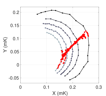
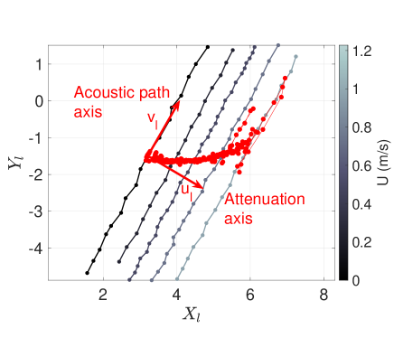
Figure 28: Experiment: measurement of a resonance with second sound tweezers at $T_{0}\approx 2.14$ K, for different values of the mean flow velocity $U$. The left panel presents the data in the phase-quadrature plane, and the right panel presents the same data after the complex inversion. The red points are obtained for a fixed value $f=6.35$ kHz, and sweeping the flow mean velocity between $0$ and $1.2$ m/s.

IV.4.2 Measure of vortex line density fluctuations

Second sound tweezers are designed to directly probe locally vortex line density fluctuations, not only its average value. The method to probe fluctuations slightly differs from the method used to probe the average value explained in sec. IV.4.1. The average VLD value can be directly computed using the complex inversion of experimental data, but this is no longer possible for its fluctuations. Indeed, the tweezers signal have different sources of noise, like e.g. thermal white noise, interfering frequencies, electromagnetic bursts, etc… Those signals can usually be considered as independent additive noises in the signal data, and easily filtered out or attenuated by an appropriate post-processing. On the contrary, the complex inversion is a non-linear transformation. Using the latter on noisy data can lead to an overestimation of the signal fluctuations closest to zero, perturb the additivity of noise sources and make them much more difficult to filter out. We thus choose to compute the VLD fluctuations only using linear transformations.

The first step is similar to that of sec. IV.4.1. We sweep the second sound frequency $f$ close to the resonant frequency $f_{0}$, in order to measure a part of the Kennelly circle. We then transform this Kennelly circle into a straight line using the complex inversion, and we find the global basis $(\mathbf{u}_{l},\mathbf{v}_{l})$ in the plane of elliptic coordinates. A fit of the Kennelly circle, and its transformation into a straight line, can be seen in Fig. 29. This experimental step has to be done just before the fluctuations’ measurement.

We then record the signal fluctuations $\left(X(t),Y(t)\right)$, for different values of the flow mean velocity $U$. Fig. 29 displays the fluctuating signal for $U=0$ and $U=1.2$ m/s in the form of clouds of data points. It can be in particular observed that the $U=1.2$ m/s data are shifted compared to the $U=0$ m/s data because of both an average attenuation and an acoustic path shift (see sec. IV.4.1). Let us define $\left\langle\mathbf{Z}(t)\right\rangle=\left\langle X(t)\right\rangle+i\left\langle Y(t)\right\rangle$ the average complex position in the phase-quadrature plane, for a given value of $U$. Following Eq. (42), the local basis $(\mathbf{u},\mathbf{v})$ of the attenuation and acoustic path axes can be computed from the global elliptic basis $(\mathbf{u}_{l},\mathbf{v}_{l})$ by

$$\begin{cases}\mathbf{u}&=-\mathbf{u}_{l}\frac{\left\langle\mathbf{Z}\right\rangle^{2}}{\left|\left\langle\mathbf{Z}\right\rangle\right|^{2}}\\ \mathbf{v}&=-\mathbf{v}_{l}\frac{\left\langle\mathbf{Z}\right\rangle^{2}}{\left|\left\langle\mathbf{Z}\right\rangle\right|^{2}}\end{cases}.$$ (47)

Fig. 29 shows that the local basis $(\mathbf{u},\mathbf{v})$ depends on $\left\langle\mathbf{Z}\right\rangle$ and thus on the value of $U$: for different mean velocities, the bases are rotated from one another. If there is a significant drift of the mean signal value during the measurement (as can e.g. be observed in Fig. 20), the local basis will also depend on time, with a typical timescale that should be much larger than the fluctuation timescale.

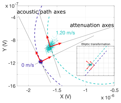
Figure 29: Illustration of the method used for fluctuations decomposition. The two patches display the fluctuating signals obtained at the mean flow velocities 0 m/s and 1,2 m/s in the X-Y plane. The inset panel displays the signal after the elliptic transformation of Fig. 27. The method to obtain the two projection axes is detailed in the main text.

The acoustic path fluctuations and the attenuation fluctuations can then be recovered using a projection on the $(\mathbf{u},\mathbf{v})$ basis. More precisely, let $x$ be the average acoustic path value and $\delta\xi=\xi-\left\langle\xi\right\rangle$ be a small fluctuation of the attenuation coefficient, a leading order expansion of expression Eq. (41) shows that

$$\overline{T}\approx\frac{A}{\sinh\left(ix+\left\langle\xi\right\rangle D\right)}-\delta\xi\frac{AD}{\sinh\left(ix+\left\langle\xi\right\rangle D\right)\tanh\left(ix+\left\langle\xi\right\rangle D\right)}.$$ (48)

We then do the approximation $\left\langle\mathbf{Z}\right\rangle\approx A/\sinh\left(ix+\left(\xi_{0}+\left\langle\xi_{VLD}\right\rangle\right)D\right)$ which is equivalent to neglecting non-linear corrections in Eq. (48). We finally get

$$\delta\xi(t)=\frac{1}{D}\mathbf{u}.\left(\mathbf{Z}(t)-\left\langle\mathbf{Z}\right\rangle\right)\times\left|\frac{\tanh\left(ix+\left(\xi_{0}+\left\langle\xi_{VLD}\right\rangle\right)D\right)}{\left\langle\mathbf{Z}\right\rangle}\right|,$$ (49)

where the value of $\xi_{0}$ can be found with Eq. (44) and $\left\langle\xi_{VLD}\right\rangle$ with Eq. (46).

The use of the elliptic method is illustrated by Figure 30, which reports the probability density function of the fluctuations of the quantum vortex density in a nearly isotropic superfluid turbulent flow The data of this plot were reported together with spectra of vorticity fluctuations. For details about the setup and analysis of these results, see WVR, 21.

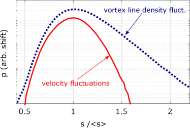
Figure 30: Example of the probability density function of vortex line density (dashed line) and velocity (continuous line) measured simultaneously by second sound tweezers in the same superfluid turbulent flow WVR (21). In abscissa, each signal $s$ is normalized by its mean value $<s>$. The nearly Gaussian velocity statistics and skewed vorticity statistics are reminiscent of those in classical turbulence.

IV.4.3 Filtering the vibration of the plates

One possible source of noise for second sound resonator measurements is the vibration of the plate arms whenever $U\neq 0$. The signature of those vibrations can be very clearly identified in the form of two thin peaks in the fluctuation power spectrum. Those two peaks are located at the two arm resonant frequencies: their exact values can vary for different tweezers, but we always observe them around $f\approx 1$ kHz (see Sec. IV.4).

Fortunately, the tweezers’ arm vibrations correspond to a variation of the gap $D$, and thus to acoustic path fluctuations. Fig. 31 displays a part of the tweezers’ fluctuation power spectrum. The fluctuations are projected along the attenuation axis (blue curve) and along the acoustic path axis (red curve), following the method presented in Sec. IV.4.2. The two peaks located at $f\approx 825$ Hz and $f\approx 1050$ Hz are identified on the acoustic path axis fluctuation power spectrum, whereas the same peaks are damped by many orders of magnitude on the attenuation axis fluctuations. These spectra illustrate the effectiveness of the elliptic method.

Using the power spectrum of Fig. 31, we can estimate the order of magnitude of the gap standard deviation. We find $\sqrt{\left\langle\left(\delta D\right)^{2}\right\rangle}\approx 0.5$ $\mu{\rm m}$, and $\frac{\sqrt{\left\langle\left(\delta D\right)^{2}\right\rangle}}{D}\approx 4\times 10^{-4}$. This confirms that the arm vibrations have a negligible impact on the measurement.

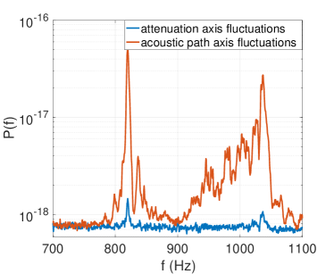
Figure 31: Experiment: a part of second sound tweezers fluctuation power spectrum, with $T_{0}=1.65$ K, $U=1.2$ m/s and for a tweezers gap $D=1.320$ mm. The tweezers’ arms resonances can be clearly identified in the acoustic path fluctuations.

IV.5 Velocity measurements

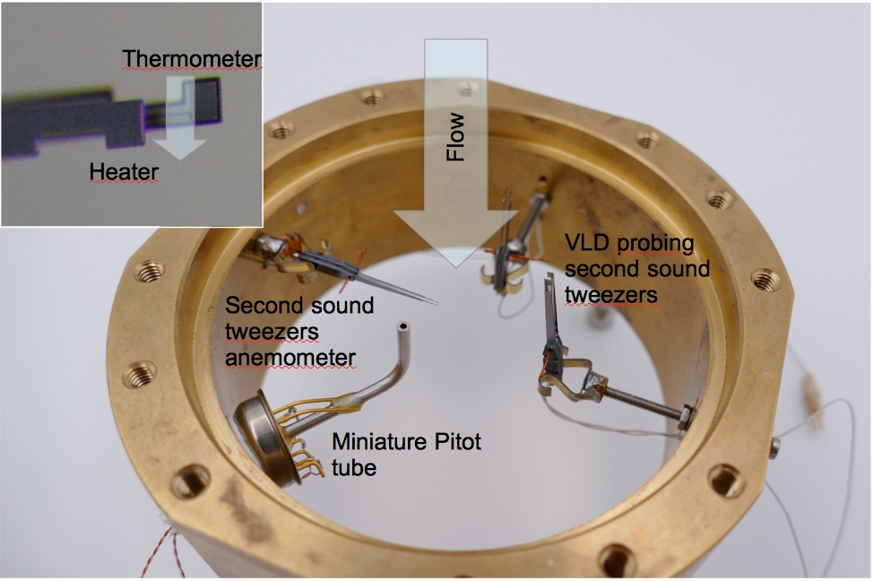
Figure 32: Example of an arrangement of three second sound tweezers dedicated to velocity (x1, left side) and vorticity (x2, right side) time series acquisitions, together with a miniature total head pressure tube (loosely labelled "Pitot tube" on the bottom left side of the picture) used for velocity calibration. All probes are mounted on a ring connecting two 76 mm-inner-diameter coaxial pipes (see Fig.1 of ref. WVR (21)). The insert is a close-up view of the shifted plates of the anemometer tweezers.

As shown in Sec. III.5, the geometry of the second sound tweezers can be optimized to sense specifically velocity rather than vortex density. One trick for achieving this is to shift one plate with respect to the other in the flow direction. Figure 32 shows three second sound tweezers and one anemometer that is based on the same principle as Pitot tubes. All sensors are positioned across a nearly homogeneous turbulent flow bounded by a cylindrical pipe (not shown here). Ffor details on this set-up, see RCSR17a, . The insert in the figure is a close-up view of the tip of the left-side tweezers, which is dedicated to velocity measurements. This shift of one plate versus the other in the downstream direction is clearly visible.

The projection of the anemometer-tweezers signal in the complex plane is not performed along orthogonal axes. These axes are determined with an in-situ calibration, ramping the mean velocity. The complementary "Pitot tube" signal is used to calibrate the axis in units of m/s.

As an illustration, Figure 30 presents the probability density function of the velocity fluctuations measured by the anemometer tweezers, together with vortex line density fluctuations recorded by the other tweezers in the same set-up (see Fig. 32). As already reported in quantum turbulence SCLR (12), the velocity statistics are close to Gaussian when probed at scales significantly larger than the intervortex distance, which is the case here. Velocity spectra derived from the same dataset are reported in WVR, 21.

V Summary and Perspectives

This study covers three independent topics: (i) the comprehensive analytical modeling of second-sound resonators with a cavity that allows a throughflow of superfluid (Section 3), (ii) new mathematical methods to process the signals provided by such resonators (Section 4), and (iii) the miniaturization of immersed second-sound resonators enabling time- and/or space-resolved flow sensing (Section 2). These miniaturized resonators, named second-sound tweezers, have been used throughout the manuscript to demonstrate the strength and limitations of the modeling and analysis methods.

Two observations remain unexplained: the origin of some noise in the acoustic path length and second-order oscillations in the resonator spectral response in quiescent ⁴He, named the "daisy effect" (section 3.4.4). Fortunately, neither effect affects the measurement of flow vorticity or velocity.

Some unexpected results have arisen from this study, and it is worthwhile to recall and discuss them.

• the possibility to operate the second-sound tweezers in a non-linear mode by over-driving the standing wave beyond an intrinsic turbulent transition. In this mode, the probe becomes sensitive to velocity, which is interpreted as a signature of the local vortex tangle being swept by the outer flow (section 2.2.3). This operating mode is analogous to hot film and hot wire anemometry in classical fluid dynamics, where sensitivity to velocity is due to the more-or-less pronounced sweeping of the thermal boundary layer around an overheated thermometer.

• In the linear regime, where the second-sound standing wave has a small amplitude, the tweezers can be designed and operated to be predominantly sensitive to either the quantized vortices or the throughflow velocity (section 3.5). This theoretical prediction is experimentally verified by comparing the statistics obtained from turbulent flows (section 4.5). The spatial and temporal resolutions of tweezers operated as anemometers, both in nonlinear and linear modes, are comparable to or better than alternative miniaturized anemometers operating in He II, such as hot-wires DBM⁺ (15); DRS⁺ (21), cantilevers SMR (12); RCSR17b , Pitot tubes SMR (12); RCSR17b , and total head-pressure probes MT (98); WVR (21).

• In the absence of throughflow, the spectral response of the resonators and its quality factors can be accurately determined by considering only the loss due to diffraction and misalignment of the reflecting plates of the cavity. Other sources of dissipation have negligible contributions under the conditions studied here. However, in the presence of a throughflow carrying quantum vortices, the vortices can significantly contribute to the total dissipation. We have not experimentally explored the production and detection of second-sound by mechanical means, which requires a cavity with rough surfaces such as millipore or nucleopore membranes. In this case, the effect of vortices pinned on the surface may no longer be negligible. For a discussion, see DLL, 80.

• The elliptic method allows the variations in vortex line density or velocity to be sensed without knowledge of the variations in second sound velocity (or acoustical path). More generally, the method enables a mathematical decoupling of both effects using a projection method in the (inverse) complex plane. This result is of significant practical interest in flows where the second-sound velocity is not accurately controlled due to residual temperature variations or thermal gradients. Such situations can occur, for instance, in flows sequentially driven at various levels of forcing (e.g., to explore Reynolds number dependence), in inhomogeneous dissipative flows, and in flows close to the lambda superfluid transitions where the second-sound velocities strongly depend on temperature.

Two applications of second-sound tweezers have been demonstrated. The small size of the probe enables measurements within a turbulent boundary layer (see Fig. 23), while the high time and spatial resolution allow for time-series measurements in the bulk of quantum turbulent flow (see Fig. 30). The probe has potential for mapping the velocity or vorticity field of inhomogeneous flows, as demonstrated by recent mapping of the vorticity in a counterflow jet ŠRLM (23).

Another potential application of tweezers is to simultaneously measure temperature fluctuations and either velocity or vorticity, enabling exploration of their correlations in turbulent counterflows or co-flows. The tweezers thermometer can provide a direct measurement of temperature within a bandwidth ranging from zero frequency up to a fraction of the frequency of the second sound standing wave, and this signal can be multiplexed with the measurement of the second sound standing wave. Alternating measurements in the linear and non-linear modes can also be useful to locally explore both velocity and vorticity in a given flow. Another possible application is to use a double-tweezers configuration consisting of a heating plate between two thermometer plates, or vice versa. Such a stack can be used to probe joint statistics of vorticity on one side and velocity on the other, or it can be used alternatively to probe transverse gradients of either vorticity or velocity.

VI Acknowledgements

*

We would like to express our gratitude to our colleague Benoît Chabaud for his support during the cryogenic tests and operation of the TOUPIE wind tunnel. We would also like to acknowledge and thank the staff of the PTA technological platform at the Minatec campus in Grenoble, France, and of the Nanofab technological platform at the Institut Néel. The data in Figure 23 were acquired in the SHREK facility, and we are grateful to all the members of the SHREK collaboration for their contributions, especially Michel Bon Mardion and Bernard Rousset for their specific operation near the superfluid transition. Finally, we acknowledge the contribution of A. Elbakyan for contributing to make our bibliography more complete.

The design, fabrication, cryogenic operation, and theoretical analysis of the probe spanned almost 7 years and were made possible by the following grants: ANR Ecouturb grant (ANR-16-CE30-0016), ANR QUTE-HPC grant (ANR-18-CE46-0013), and the EU Horizon 2020 Research and Innovation Program, "the European Microkelvin Platform" (EMP 824109).

Appendix A Micro-fabrication process

The cantilevers’ fabrication process is presented in Fig. 33 and summarized below.

Figure 33: Cantilevers’ fabrication process.

Step 1: Starting substrateThe cantilevers were fabricated by processing SOI (Silicon On Insulator) wafers by microelectronic techniques. The thicknesses of the device, buried oxide and silicon substrate layers were respectively 20 µm, 1 µm and 500 µm. The wafers diameters were 100 mm. The wafers were double side polished and were oxidized to form a 100 nm thick SiO₂ layer on both sides.

Step 2: Electrical path fabricationThe serpentine electrical path (red color) was deposited first on the SOI wafer frontside. The deposition was done using a standard photolithography, evaporation and lift-off sequence. The photoresist model was AZ 5214E from Microchemicals GmbH, processed as a negative photoresist. Depending on the cantilever type, heater or thermometer, two different evaporation sequences were used: Ti 5 nm + Pt 80 nm or Au 25 nm + Sn 100 nm. Evaporation was preceded by in situ wafer surface cleaning by an argon ions bombardment during 20 s. Lift-off was initiated in an acetone bath during 5 min and then completed by ultrasounds during a few tens of seconds.

The current leads (orange color) were deposited during a second photolithography, evaporation and lift-off sequence. The evaporation sequence was Ti 5 nm + Au 200 nm + Ti 5 nm + Pt 50 nm. The usage of a platinum layer was found to facilitate lift-off and may also be useful for brazing purpose. A thin protective resist layer was deposited on frontside in order to protect it during all subsequent operations on the backside.

Steps 3-4: Backside masks fabricationIn order to etch silicon from the backside, two superimposed etch masks were fabricated. First, an aluminum mask was made by a photolithography, evaporation and lift-off sequence on the wafer backside. A double-side alignment was necessary during photolithography. The aluminum thickness was 120 nm. The protective resist layer on frontside had to be deposited again after lift-off.

Then, a resist mask was deposited over the aluminum one. This mask was made by photolithography on the positive AZ4562 photoresist spin-coated at 4000 rpm.

The aluminum mask was identical to the resist mask except within the arm area, as shown in Fig. 33. This area was covered by resist, but not by aluminum.

Step 5: Backside etching 1The etch mask during this phase was the resist mask (see step 4 in Fig. 33). The area exposed to etching includes the tip area and a 200 µm wide trench which delimits the piece contour. First, the thin surface oxide layer was etched by reactive ion etching (RIE) based on SF₆ gas. Then, the silicon was etched in a STS HRM deep reactive ion etching (DRIE) equipment using a standard recipe based on Bosch process. The etch rate was around 10 µm/min, the etched depth was around 230 µm (120 cycles). The longer this phase, the thicker the cantilever arm at the end of the process.

Steps 6-7: Backside etching 2Following the first silicon etch phase, the resist mask was removed by an oxygen plasma, thus uncovering the arm area and the remaining aluminum etch mask. The area exposed to etching includes the previous one plus the arm area. The backside surface oxide was etched into the arm area. Then, another silicon etch sequence was applied with the aluminum mask. This sequence was stopped when the buried oxide was reached everywhere in the tip area and in the cantilever contour (NOT in the arm area). The same recipe was used, 200 cycles were applied.

An additional difficulty appeared at this step due to a parasitic effect during etching. This effect originates from the polymer passivation layer deposited on sidewalls during the first silicon etch phase. As the arm area was masked during the first silicon etch sequence and unmasked during the second one, the passivation layer located along the arm edges was released and generated locally some irregular micromasking effect. In order to decrease the micromasking, the etch recipe was interrupted 3 times, every 50 cycles, in order to apply a 1 min oxygen plasma followed by 20 s of an isotropic silicon etching recipe.

The final 50 etching cycles ended up reaching the buried oxide layer, at the trench bottom, all around the cantilever. It is necessary at this step to check that the buried oxide is fully uncovered by silicon everywhere in the trench bottom and in the tip area. However, etching cycles should not be applied in excess to avoid some mechanical weakening of the wafer.

Phase	Deposition	Etch
Sub-phase	Main	Delay	Boost	Main
Gas	C4F8: 250 sccm	SF6: 250 sccm O2: 10 sccm
Duration	3 s	2.0 s	5.5 s	22.5 s
Pressure	14 mTor	20 mTor	40 mTor	40 mTor
Coil power	300 W	300 W	300 W	1 W
Platen power	20 W	100 W	50 W	1 W
Electroma-
gnet current	0 A	0 A	2 A	0 A
Platen
frequency	RF 13.56 MHz
He backside
pressure	10 Tor

Table 2: Bosch process recipe used during frontside deep silicon etching.

Steps 8-9: Buried oxide etchingThe buried oxide was then removed by plasma etching. This oxide was fully removed at the trench bottom and in the tip area. If this layer is not removed, some bending may occur on the tip at the end of the process, due to mechanical stress of oxide. The aluminum mask was removed in an aluminum etchant solution at 50 °C during a few minutes.

Steps 10-12: Frontside etchingThe frontside protective resist layer was removed during an acetone cleaning bath. The 3D cantilever structuration was ended by a third silicon etching made from the frontside. The etch mask was formed by photolithography on AZ1512HS resist, deposited at 4000 rpm. As shown on Fig. 33, the mask design includes two bridges on the baseplate sides in order to maintain the cantilever after having opened the trench that surrounds it. The design also includes the tip contour. The frontside thin surface oxide was etched first, then the silicon of the device layer. The silicon etching was done with specific conditions. Due to the wafer mechanical weakness at this step, caused by the multiple deep trenches made on the backside, the processed wafer was attached to a blank silicon wafer by Kapton tape. This ensemble was loaded into the etching chamber. As no thermal bridge was present between the two wafers, the recipe was adapted: low RF powers were used and a 22 s idle time was added after each etching cycle (see table 2). The objective was to avoid overheating during etching. The silicon etch duration was 50 cycles. After this sequence, the trench around the cantilever was fully opened. The resist was removed by a low power oxygen plasma.

References

- Bal [07] S Balibar. The discovery of superfluidity. Journal of Low Temperature Physics, 146(5-6):441–470, 2007.
- Ben [22] Charles A Bennett. Principles of physical optics. John Wiley & Sons, 2022.
- BLR [17] J. Bertolaccini, E. Lévèque, and P.-E. Roche. Disproportionate entrance length in superfluid flows and the puzzle of counterflow instabilities. Phys. Rev. Fluids, 2:123902, 2017.
- BSS [83] H Borner, T Schmeling, and DW Schmidt. Experimental investigations on fast gold-tin metal film second-sound detectors and their application. J. Low Temp. Phys., 50(5):405–426, 1983.
- BVS+ [14] S Babuin, E Varga, L Skrbek, E Lévêque, and P-E Roche. Effective viscosity in quantum turbulence: A steady-state approach. EPL, 106(2):24006, 2014.
- CA [68] R W. Cohen and B Abeles. Superconductivity in granular aluminum films. Phys. Rev., 168:444–450, 1968.
- CCCH [00] O. Chanal, B. Chabaud, B. Castaing, and B. Hébral. Intermittency in a turbulent low temperature gaseous helium jet. Eur. Phys. J. B, 17:309–317, 2000.
- CCH [92] B. Castaing, B. Chabaud, and B. Hebral. Hot-wire anemometer operating at cryogenic temperatures. Rev. Sci. Instrum., 63:4167–4173, 1992.
- CR [83] M J Crooks and B J Robinson. Technique for determining second sound attenuation near the superfluid transition in 4He. Review of Scientific Instruments, 54(1):12–15, 1983.
- CSW [78] John C Cummings, Dieter W Schmidt, and Wolfgang J Wagner. Experiments on second-sound shock waves in superfluid helium. Phys. Fluids, 21:713, May 1978.
- DB [98] R J Donnelly and C F Barenghi. The observed properties of liquid helium at the saturated vapor pressure. Journal of physical and chemical reference data, 27(6):1217–1274, 1998.
- DBM+ [15] D. Durì, C. Baudet, J.-P. Moro, P.-E. Roche, and P. Diribarne. Hot-wire anemometry for superfluid turbulent coflows. Review of Scientific Instruments, 86(2):025007, 2015.
- Des [86] Pramond D Desai. Thermodynamic properties of iron and silicon. Journal of physical and chemical reference data, 15(3):967–983, 1986.
- DL [77] P E Dimotakis and G A Laguna. Investigations of turbulence in a liquid helium II counterflow jet. Physical Review B, 15:5240, Jun 1977.
- DLF+ [14] Q. Dong, Y. X. Liang, D. Ferry, A. Cavanna, U. Gennser, L. Couraud, and Y. Jin. Ultra-low noise high electron mobility transistors for high-impedance and low-frequency deep cryogenic readout electronics. Applied Physics Letters, 105(1):013504, 2014.
- DLL [80] D D’Humières, A Launay, and Albert Libchaber. Pinning of vortices in nucleopores. effect on second-sound resonators. Journal of Low Temperature Physics, 38:207, Jan 1980.
- Don [91] R. J. Donnelly. Quantized Vortices in Helium-II. Cambridge Studies in Low Temperature Physics. Cambridge University Press, Cambridge, 1991.
- Don [09] Russell J Donnelly. The two-fluid theory and second sound in liquid helium. Phys. Today, 62(10):34–39, 2009.
- DRS+ [21] P. Diribarne, B. Rousset, Y. A. Sergeev, J. Valentin, and P.-E. Roche. Cooling with a subsonic flow of quantum fluid. Physical Review B, 103(14):144509, 2021.
- FS [04] S Fuzier and Steven W Van Sciver. Use of the bare chip cernox(tm) thermometer for the detection of second sound in superfluid helium. Cryogenics, 44:211, Mar 2004.
- Goo [05] Joseph W Goodman. Introduction to Fourier optics. Roberts and Company publishers, 2005.
- Gri [09] A Griffin. New light on the intriguing history of superfluidity in liquid 4He. Journal of Physics: Condensed Matter, 21(16):164220, 2009.
- GSB+ [09] F. Gauthier, J. Salort, O. Bourgeois, J.-L. Garden, R. du Puits, A. Thess, and P.-E. Roche. Transition on local temperature fluctuations in highly turbulent convection. EPL, 87:44006, 2009.
- HL [88] K Henjes and M Liu. Peshkov transducers of second sound. Journal of Low Temperature Physics, 71(1):97–117, 1988.
- HR [76] J Heiserman and I Rudnick. The acoustic modes of superfluid helium in a waveguide partially packed with superleak. Journal of Low Temperature Physics, 22(5):481–499, 1976.
- [26] H. E Hall and W. F Vinen. The rotation of liquid Helium II. i. experiments on the propagation of second sound in uniformly rotating Helium II. Proceedings of the Royal Society of London. Series A, 238:204, Dec 1956.
- [27] H. E Hall and W. F Vinen. The rotation of liquid Helium II. II. the theory of mutual friction in uniformly rotating helium II. Proceedings of the Royal Society of London. Series A, 238:215, Dec 1956.
- HVS [92] D. S. Holmes and S. W. Van Sciver. Attenuation of second sound in bulk flowing He II. J. Low Temp. Phys., 87:73–93, 1992.
- HVS [01] D.K. Hilton and S.W. Van Sciver. Techniques for the detection of second sound shock pulses and induced quantum turbulence in He II. Cryogenics, 41:347–53, 2001.
- JL [63] Robert Chandler Johnson and WA Little. Experiments on the kapitza resistance. Physical review, 130(2):596, 1963.
- Kem [91] R. C. Kemp. The reference function for platinum resistance thermometer interpolation between 13,8033 K and 273,16 K in the international temperature scale of 1990. Metrologia, 28(4):327, 1991.
- Kha [00] I M Khalatnikov. An Introduction to the Theory of Superfluidity. CRC Press, 2000.
- Lag [76] G. Laguna. Photolithographic fabrication of high frequency second sound detectors. Cryogenics, 16(4):241–243, 1976.
- LFF [47] C. T. Lane, Henry A. Fairbank, and William M. Fairbank. Second sound in liquid Helium II. Phys. Rev., 71:600–605, May 1947.
- Lob [07] N Lobontiu. Dynamics of microelectromechanical systems. Springer, Boston, MA, 2007.
- LV [74] D Lhuillier and F Vidal. Temperature dependence of the second sound velocity reduction in rotating liquid helium. Journal of Physics C: Solid State Physics, 7(14):L254, 1974.
- Meh [74] J. B Mehl. New effects in the interaction of second sound with superfluid vortex lines. Physical Review A, 10(2):601, 1974.
- MG [18] B Mastracci and W Guo. An apparatus for generation and quantitative measurement of homogeneous isotropic turbulence in he ii. Review of Scientific Instruments, 89(1):015107, 2018.
- MLM [78] RJ Miller, IH Lynall, and JB Mehl. Velocity of second sound and mutual friction in rotating helium II. Physical Review B, 17(3):1035, 1978.
- MMP+ [07] V. F Mitin, PC McDonald, F Pavese, NS Boltovets, VV Kholevchuk, IY Nemish, VV Basanets, VK Dugaev, PV Sorokin, and RV Konakova. Ge-on-gaas film resistance thermometers for cryogenic applications. Cryogenics, 47(9-10):474–482, 2007.
- MPS [84] P Mathieu, B Plaçais, and Y Simon. Spatial distribution of vortices and anisotropy of mutual friction in rotating He II. Physical Review B, 29:2489, Mar 1984.
- MSS [76] P. Mathieu, A. Serra, and Y. Simon. Critical-region measurements of the mutual-friction parameters in rotating He II. Phys. Rev. B, 14:3753–3761, 1976.
- MSS [21] Š Midlik, D Schmoranzer, and L Skrbek. Transition to quantum turbulence in oscillatory thermal counterflow of he 4. Physical Review B, 103(13):134516, 2021.
- MT [98] J. Maurer and P. Tabeling. Local investigation of superfluid turbulence. Europhys. Lett., 43(1):29–34, 1998.
- NF [95] S. K. Nemirovskii and W. Fiszdon. Chaotic quantized vortices and hydrodynamic processes in superfluid helium. Rev. Modern Phys., 67:37–84, 1995.
- [46] Phosphor bronze wire, a positive temperature coefficient thermometer, has also been used in the early days [53].
-
[47]
In one dataset, a small discontinuity in the versus dependence around
W/cm2
was observed in the quasi-linear region of quiescent superfluid around
1.5\tmspace+.2222emK (not shown), suggesting another
flow transition, but this effect was not detectable in other datasets. The
Reynolds number of this possible transition can be defined using the
transverse characteristic length scale mm, the quantum of circulation m2/s, and the
counterflow superfluid velocity towards the heater mm/s (amplification of velocity by the quality
factor of the cavity has not been taken into account). One finds
Critical Reynolds numbers of a few units have already been reported to characterize the threshold of the appearance of a few superfluid vortices across the section of pipes that are closed at one of their ends with a heating plug (see Fig. 3 in [3]), a transition referred to as the T1-transition in the counterflow literature[77, 45]. By analogy, this could suggest that the discontinuity at might be associated with the appearance of a sparse tangle of quantum vortices near the heater, which density is expected to increase at larger . Such vortices would damp the standing wave, but no such effect has been detected. Indeed, the observed damping of the standing wave in quiescent He\tmspace+.2222emII can be accounted for by the sole effect of diffraction (as shown later), indicating that all the other sources of loss are comparatively small. Loss due to such “counterflow” vortices would make the dependence sub-linear rather than linear, which is not clearly observed. Since no quantitative evidence of these vortices could be clearly identified, this effect was not further explored. - [48] Advection of second sound by velocity is illustrated e.g. in [14].
- [49] This result confirms the analysis of the first dataset measured using a second sound tweezer, in 2007[63].
-
[50]
In this case, the complex amplitude of the nth temperature resonance is
often approximated by the Lorentzian formula [82, 16]
where , and are the amplitude at resonance, the quality factor and resonance frequency of the mode of interest. To highlight that this Lorentzian approximation describes a circle in the complex plane -, it can be written as:(50)
where and . - Not [64] H A Notarys. Megacycle frequency second sound. PhD thesis, California Institute of Technology, 1964.
- OP [94] JR Olson and RO Pohl. Kapitza resistance between silicon and helium-4. Journal of low temperature physics, 94:539–550, 1994.
- Pes [46] V. P. Peshkov. Determination of the velocity of propagation of the second sound in helium II. Journal of Physics (Moscow), 10:389, 1946.
- Pes [48] VP Peshkov. Propagation of second sound in helium II. exp. Zh. Eksp. Teor. Fiz., 18:857, 1948.
- PGB [70] R. L St Peters, T. J. Greytak, and G.B. Benedek. Brillouin scattering measurements of the velocity and attenuation of high frequency sound waves in superfluid helium. Optics Communications, 1(9):412–416, 1970.
- PK [82] DB Poker and CE Klabunde. Temperature dependence of electrical resistivity of vanadium, platinum, and copper. Physical Review B, 26(12):7012, 1982.
- Pol [69] Gerald L. Pollack. Kapitza resistance. Reviews of Modern Physics, 41(1):48–81, 1969.
- PPB+ [03] S Pietropinto, C Poulain, C Baudet, Bernard Castaing, Benoît Chabaud, Y Gagne, Bernard Hébral, Y Ladam, P Lebrun, O Pirotte, and P.-E. Roche. Superconducting instrumentation for high Reynolds turbulence experiments with low temperature gaseous helium. Physica C, 386:512, Apr 2003.
- Put [74] S J Putterman. Superfluid hydrodynamics. Series in low temperature physics, 3, 1974.
- RBD+ [14] B. Rousset, P. Bonnay, P. Diribarne, A. Girard, J.M. Poncet, E. Herbert, J. Salort, C Baudet, B Castaing, L. Chevillard, F. Daviaud, B. Dubrulle, Y. Gagne, M. Gibert, B. Hébral, T. Lehner, P.-E. Roche, B. Saint-Michel, and M Bon Mardion. Superfluid high Reynolds von Kármán experiment. Rev. Sci. Instrum., 85:103908, 2014.
- [61] E Rusaouen, B Chabaud, J Salort, and P-E Roche. Intermittency of quantum turbulence with superfluid fractions from 0% to 96%. Phys. Fluids, 29(10):105108, 2017.
- [62] E. Rusaouen, B. Chabaud, J. Salort, and P.-E. Roche. Intermittency of quantum turbulence with superfluid fractions from 0% to 96%. Phys. Fluids, 29(10):105108, 2017.
- RDD+ [07] P-E Roche, Pantxo Diribarne, Thomas Didelot, Olivier Français, Lionel Rousseau, and Hervé Willaime. Vortex density spectrum of quantum turbulence. EPL (Europhysics Letters), 77(6):66002, 2007.
- RG [84] M. Raui and A. Guenter. Damping of second sound near the superfluid transition of 4He as a function of pressure. Physical Review B, 30:5116, Nov 1984.
- RR [01] D Rinberg and M L Rappaport. Fiber bolometer and emitter with negligible reflection for second sound measurements near the lambda-point. Cryogenics, 41(8):557–561, 2001.
- RVA [16] Aymeric Ramiere, Sebastian Volz, and Jay Amrit. Thermal resistance at a solid/superfluid helium interface. Nature materials, 15(5):512–516, 2016.
- Sad [98] J E Sader. Frequency response of cantilever beams immersed in viscous fluids with applications to the atomic force microscope. Journal of Applied Physics, 84(1):64–76, 1998.
- SCLR [12] J. Salort, B. Chabaud, E. Lévêque, and P.-E. Roche. Energy cascade and the four-fifths law in superfluid turbulence. EPL, 97:34006, 2012.
- SE [70] R. A Sherlock and D. O Edwards. Oscillating superleak second sound transducers. Rev. Sci. Instrum., 41:1603, Jan 1970.
- SHVS [99] M.R. Smith, D.K. Hilton, and S. W. Van Sciver. Observed drag crisis on a sphere in flowing He I and He II. Phys. Fluids, 11:751–3, 1999.
- SMR [12] J. Salort, A. Monfardini, and P.-E. Roche. Cantilever anemometer based on a superconducting micro-resonator: Application to superfluid turbulence. Rev. Sci. Instrum., 83:125002, 2012.
- SNVD [02] S.R. Stalp, J. J Niemela, W. J. Vinen, and R. J. Donnelly. Dissipation of grid turbulence in helium II. Phys. Fluids, 14:1377–9, 2002.
- Sny [62] H. A. Snyder. Use of germanium as a second sound receiver. Review of Scientific Instruments, 33(4):467–469, 1962.
- SP [66] H. A. Snyder and Zimri Putney. Angular dependence of mutual friction in rotating Helium II. Phys. Rev., 150:110, 1966.
- SPB [17] GW Stagg, NG Parker, and CF Barenghi. Superfluid boundary layer. Physical Review Letters, 118(13):135301, 2017.
- ŠRLM [23] P Švančara, P.-E. Roche, and M. La Mantia. Spatial distribution of the quantized vortices’ tangle in thermally driven round jets of superfluid helium. Phys. Fluids, 35:035136, 2023.
- Tou [82] J. T. Tough. Superfluid Turbulence, volume 8, chapter 3, pages 133–219. North-Holland Publishing Company, Amsterdam, 1982.
- Tsa [62] D.S. Tsakadze. (sov. phys. jetp 15 (1962) 681). Zh. Eksp. Teor. Fiz., 42:985, 1962.
- VBL+ [17] E Varga, S Babuin, VS L’vov, Anna Pomyalov, and L Skrbek. Transition to quantum turbulence and streamwise inhomogeneity of vortex tangle in thermal counterflow. Journal of Low Temperature Physics, 187(5-6):531–537, 2017.
- Vin [57] W. F Vinen. Mutual friction in a heat current in liquid helium II. iii. theory of the mutual friction. Proceedings of the Royal Society of London. Series A, 242:493, Nov 1957.
- VJSS [19] E Varga, MJ Jackson, D Schmoranzer, and L Skrbek. The use of second sound in investigations of quantum turbulence in He II. J. Low Temp. Phys., 197(3):130–148, 2019.
- VS [71] F Vidal and Y Simon. Ideal second sound resonance in He-II. Physics Letters A, 36(3):165–166, 1971.
- WBF+ [69] R. Williams, S.E.A. Beaver, J.C. Fraser, R.S. Kagiwada, and I. Rudnick. The velocity of second sound near tlambda. Physics Letters A, 29(5):279–280, 1969.
- WPHE [81] P. E. Wolf, B. Perrin, J. P. Hulin, and P. Elleaume. Rotating Couette flow of helium II. J. Low Temp. Phys., 44:569–593, September 1981.
- WVR [21] E Woillez, J Valentin, and P-E Roche. Local measurement of vortex statistics in quantum turbulence. EPL (Europhysics Letters), 134(7):46002, 2021.
- YI [18] J Yang and GG Ihas. Decay of grid turbulence in superfluid helium-4: Mesh dependence. In Journal of Physics: Conference Series, volume 969, page 012004. IOP Publishing, 2018.
- YIE [17] J. Yang, G. G Ihas, and D. Ekdahl. Second sound tracking system. Review of Scientific Instruments, 88(10):104705, 2017.
- YYK [97] T Yotsuya, M Yoshitake, and T Kodama. Low-temperature thermometer using sputtered zrnx thin film. Cryogenics, 37(12):817–822, 1997.