Strong gravitational lensing’s ‘external shear’ is not shear

Abstract

The distribution of mass in galaxy-scale strong gravitational lenses is often modelled as an elliptical power law plus ‘external shear’, which notionally accounts for neighbouring galaxies and cosmic shear. We show that it does not. Except in a handful of rare systems, the best-fit values of external shear do not correlate with independent measurements of shear: from weak lensing in 45 Hubble Space Telescope images, or in 50 mock images of lenses with complex distributions of mass. Instead, the best-fit shear is aligned with the major or minor axis of 88% of lens galaxies; and the amplitude of the external shear increases if that galaxy is disky. We conclude that ‘external shear’ attached to a power law model is not physically meaningful, but a fudge to compensate for lack of model complexity. Since it biases other model parameters that are interpreted as physically meaningful in several science analyses (e.g. measuring galaxy evolution, dark matter physics or cosmological parameters), we recommend that future studies of galaxy-scale strong lensing should employ more flexible mass models.

1 Introduction

Gravitational lensing is the deflection of light rays by nearby concentrations of matter and their associated gravitational fields. If the light ray should pass straight through an object as massive as a galaxy, it can be deflected along multiple routes around the galaxy, and appear distorted into arcs or an ‘Einstein ring’. Such galaxy-scale strong lensing has been used to infer the distribution of mass in massive elliptical galaxies (Gavazzi et al., 2007; Koopmans et al., 2009; Auger et al., 2010; Sonnenfeld et al., 2013; Bolton et al., 2012; Etherington et al., 2023), to infer their dark matter content, stellar mass-to-light ratios, and inner structure (Massey et al., 2010; Sonnenfeld et al., 2012; Oldham & Auger, 2018; Nightingale et al., 2019; Shu et al., 2015, 2016a). If the background source is variable, measurements of time delays between multiple images can be used to measure cosmological parameters (Kilbinger, 2015) or the Hubble constant (Suyu et al., 2017; Wong et al., 2019; Harvey, 2020; Gomer & Williams, 2021). If the lens galaxy contains small substructures, which would be a smoking gun of the ‘clumpy’ Cold Dark Matter (CDM) model, they would also perturb the multiple images (Natarajan & Springel, 2004; Vegetti et al., 2010, 2014; Li et al., 2016, 2017; Hezaveh et al., 2016; Ritondale et al., 2019; Despali et al., 2019; He et al., 2022a, b; Amorisco et al., 2022; Nightingale et al., 2023a).

When modelling the distribution of mass to fit strong lensing data, two additional free parameters are frequently included. The (amplitude and angle of) ‘external shear’ is intended to represent the cumulative deflection of light by all other gravitational potentials along the line of sight. Indeed, the best-fit value of external shear matched a model of the line of sight for three of six galaxy lenses studied by Wong et al. (2011). Subsequent papers have even proposed using external shear as relatively high signal-to-noise measurements of the ‘cosmic’ shear along individual lines of sight (Birrer et al., 2017; Desprez et al., 2018; Kuhn et al., 2020; Fleury et al., 2021; Hogg et al., 2022). However, the best-fit values of external shear did not match the lines of sight to the three other galaxies studied by Wong et al. (2011) — and, in general, best-fit values are much larger than expected for both galaxy lenses (Keeton et al., 1997; Witt & Mao, 1997; Hilbert et al., 2007; Suyu et al., 2010; Barrera et al., 2021) and cluster lenses (Robertson et al., 2020; Limousin et al., 2022). Using mock observations, Cao et al. (2022, hereafter C22) demonstrated that the best-fit shear can be incorrect if the model of the mass distribution is missing complexity.

In this paper we compare the external shear measured from Hubble Space Telescope (HST) imaging — of strong lensing galaxies from the SLACS survey (Bolton et al., 2008a), GALLERY survey (Shu et al., 2016b), and four lenses in clusters — against independent measurements of the shear along the same line-of-sight, observed as weak lensing of adjacent galaxies. To gain understanding, we also analyse C22’s mock HST imaging, generated without external shear, but fitted with shear as a free parameter.

Comparing independent measurements of shear will test the hypothesis that strong lensing external shear is a real, physical quantity. Strong and weak lensing measurements average over different spatial scales and are obtained at different redshifts, so they might not be identical; but they should be strongly correlated. Analysing three lenses in the COSMOS field (Faure et al., 2008) with sophisticated statistics, Kuhn et al. (2020) measured a smaller covariance between strong and weak lensing shears than the difference between individual systems, indicating that more data were required. In this work, with a much larger sample of galaxies, we simply aim to detect a correlation between the two probes.

We define relevant concepts from lensing theory in Section 2. We then describe our observed and mock data in Section 3 and our analysis methods in Section 4. We present our results in Section 5 and investigate possible causes in Section 6. We interpret these in a wider context and conclude in Section 7. Throughout this paper, we assume a Planck 2015 cosmological model (Ade et al., 2016).

2 Gravitational lensing theory

Gravitational lensing describes the deflection of light rays from distant sources, by matter along its path to an observer, through angle $\bm{\alpha}$. This maps 2D coordinates of light on the distant source plane $\bm{\beta}$ to coordinates where they are observed on the foreground image plane $\bm{\theta}=(\theta_{1},\theta_{2})$, via the lens equation

$$\bm{\beta}=\bm{\theta}-\bm{\alpha}(\bm{\theta}).$$ (1)

If the gravitational lens is much thinner than its angular diameter distance from the observer $D_{\rm l}$, its distribution of mass can be treated as a 2D surface density projected along the line-of-sight $\Sigma(\bm{\theta})=\int\rho(D_{\rm l}\theta_{1},D_{\rm l}\theta_{2},z)\,dz$. Following the notation of Narayan & Bartelmann (1996), the deflection angle $\bm{\alpha}=\bm{\nabla}\psi$ is the vector gradient of a 2D lensing potential

$$\psi(\bm{\theta}) \equiv 2\frac{D_{\rm ls}}{D_{\rm l}D_{\rm s}}\frac{2G}{c^{2}}\int\Sigma(\bm{\theta}^{\prime})\ln{|\bm{\theta}-\bm{\theta}^{\prime}|}~{}d^{2}\bm{\theta}^{\prime}$$ (2)

$$=2\frac{D_{\rm ls}}{D_{\rm l}D_{\rm s}}\int\Phi(D_{\rm l}\bm{\theta},z)~{}dz~{},$$ (3)

where $\Phi$ is the 3D Newtonian potential, and the prefactor (which involves angular diameter distances to the lens, to the source, and from the lens to the source) reflects the geometrical efficiency of a lens: peaking if it is half-way between the source and the observer.

The Jacobian of the lens equation (1) is thus

$$A_{ij}\equiv\frac{\partial\beta_{i}}{\partial\theta_{j}}=\delta_{ij}-\frac{\partial\alpha_{i}}{\partial\theta_{j}}=\delta_{ij}-\frac{\partial^{2}\psi}{\partial\theta_{i}\theta_{j}}.$$ (4)

2.1 Weak lensing

If the source is much smaller than the scale of local variations in the gravitational field, the Jacobian can be approximated as constant

$$A_{ij} \approx\begin{pmatrix}1-\kappa-\gamma_{1}&-\gamma_{2}\\ -\gamma_{2}&1-\kappa+\gamma_{1}\end{pmatrix}$$ (5)

$$=(1-\kappa)\begin{pmatrix}1&0\\ 0&1\end{pmatrix}-\gamma\begin{pmatrix}\mathrm{cos}2\phi&\mathrm{sin}2\phi\\ \mathrm{sin}2\phi&\mathrm{cos}2\phi\end{pmatrix},$$ (6)

where the convergence

$$\kappa=\frac{1}{2}\bm{\nabla}^{2}\psi~{},$$ (7)

and where the two components of shear

$$\Big{(}\gamma_{1},~{}\gamma_{2}\Big{)}=\left(\frac{1}{2}\left(\frac{\partial^{2}\psi}{\partial\theta_{1}^{2}}-\frac{\partial^{2}\psi}{\partial\theta_{2}^{2}}\right),~{}\frac{\partial^{2}\psi}{\partial\theta_{1}\partial\theta_{2}}\right)$$ (8)

can also be expressed in terms of shear amplitude $\gamma^{2}=\gamma_{1}^{2}+\gamma_{2}^{2}$ and angle $\phi=\,$½$\,\arctan{(\gamma_{2}/\gamma_{1})}$. The convergence magnifies a source, and the shear changes its shape. Strictly, these quantities are only observable in combination as ‘reduced shear’ $g_{i}={\gamma_{i}}/{(1-\kappa)}$. However, in the weak lensing regime, $\kappa\ll 1$, so $g_{i}\approx\gamma_{i}$.

2.2 Strong lensing

If light from one side of a source is deflected differently to light from the other side, it can appear distorted in the image plane as an arc; it is also possible to see multiple images of a single source, if more than one solution exists with different $\bm{\alpha}$ and $\bm{\theta}$. To reconstruct $\bm{\alpha}(\bm{\theta})$ it is usual to note that

$$\kappa(\bm{\theta}) =\frac{\Sigma(\bm{\theta})}{\Sigma_{\mathrm{crit}}} \mathrm{with~{}constant} \Sigma_{\mathrm{crit}}= \frac{{\rm c}^{2}}{4{\rm\pi}{\rm G}}\frac{D_{\rm s}}{D_{\rm l}D_{\rm ls}}\,,$$ (9)

which is equal to the mean surface mass density within the Einstein radius, $R_{\mathrm{Ein}}$. For axisymmetric lenses the Einstein radius is uniquely defined by the radius of the circular tangential critical curve that is produced where the magnification diverges in the lens plane. This occurs where the tangential eigenvalue of the Jacobian (equation 4) $\lambda_{\mathrm{t}}=1-\kappa-\gamma$ is equal to zero. For asymmetric lenses, the definition of Einstein radius must be generalised; we choose to use the effective Einstein radius

$$R_{\mathrm{Ein,eff}}=\sqrt{\frac{A}{\mathrm{\pi}}},$$ (10)

where $A$ is the area enclosed by the tangential critical curve.

When considering (typically Early-type) galaxy-scale lenses, it is common practise to parameterise the surface mass distribution as an elliptical power law (Suyu, 2012)

$$\Sigma(\theta_{1},\theta_{2};b,q,\gamma)=\frac{3-\gamma}{1+q}\left(\frac{b}{\sqrt{\theta_{1}^{2}+\theta_{2}^{2}/q^{2}}}\right)^{\gamma-1},$$ (11)

where $b\geq 0$ is the angular scale length (referred to in some papers as the Einstein radius, but distinct from the more robust effective Einstein radius in Equation 10), $0<q\leq 1$ is the projected minor to major axis ratio of the elliptical isodensity contours, and (confusingly denoted) $\gamma$ is the logarithmic slope of the mass distribution in 3D (for an ‘isothermal’ distribution, $\gamma=2$). If we also allow the mass to be translated to central coordinates $(\theta_{1}^{\rm c},\theta_{2}^{\rm c})$ and reoriented to position angle $\phi^{\mathrm{PL}}$, which we measure counterclockwise from the positive $\theta_{1}$-axis, the model has six free parameters.

The primary lens may not be the only source of shear. Any ‘external’ component due to other galaxies or clusters near the lens or along the ray path, and constant on scales larger than $b$ (rather than the size of the source) is modelled as two more free parameters

$$\Big{(}\gamma^{\mathrm{ext}}_{1},~{}\gamma^{\mathrm{ext}}_{2}\Big{)}=\gamma^{\mathrm{ext}}\Big{(}\cos{(2\phi^{\mathrm{ext}})},~{}\sin{(2\phi^{\mathrm{ext}})}\Big{)}~{},$$ (12)

where $\gamma^{\mathrm{ext}}$ is the amplitude and $\phi^{\mathrm{ext}}$ is the angle of the shear measured counterclockwise from the $\theta_{1}$-axis. This is applied as an additional component of $\bm{\alpha}(\bm{\theta})$. It does not change $\kappa(\bm{\theta})$.

3 Data

3.1 Mock lens galaxies

We analyse a set of 50 mock lens images, representative of data from the SLACS survey. They were generated by C22 for an investigation into the systematic errors induced by the elliptical power-law model. We summarise the simulation procedure below; a detailed description can be found in Section 2.4 of that paper.

The surface mass density of the lens galaxy comprises two components: a dark matter halo, parameterised by the spherical generalised Navarro, Frenk & White (gNFW) profile (Navarro et al., 1997; Zhao, 1996; Cappellari et al., 2013), plus visible stellar matter, parameterised by a Multiple Gaussian Expansion (MGE; Cappellari, 2002). The model parameters of the gNFW and MGE profiles of each lens galaxy are set to the best-fit parameters from fits of these distributions to SDSS-MaNGA stellar dynamics data, derived by Li et al. (2019) using the Jeans anisotropic model (JAM) method. The position angle of each Gaussian component in the MGE is fixed, however their axis ratios are free to vary, allowing for elliptical gradients in the mass distribution.

The light distribution of the source galaxy is modelled by a single Sérsic profile (Graham & Driver, 2005) with effective radius $R_{\mathrm{eff}}=0.15\arcsec$, Sérsic index $n=1$, and axis ratio $q=0.7$. The position in the source plane $(x_{s},y_{s})$ is drawn from a Gaussian distribution with mean 0$\arcsec$ and standard deviation 0.1$\arcsec$, and the position angle is uniformly selected between $0^{\circ}-180^{\circ}$. The light from the source galaxy is ray-traced from the source plane at $z=0.6$ to the image plane through the lens equation (equation 1), to simulate its lensed appearance. Further, to mimic observational effects, the image is convolved with a Gaussian PSF with 0.05$\arcsec$ standard deviation, and sampled by 0.05$\arcsec$ square pixels. A flat background sky of 0.1 electrons per second is assumed, and an exposure time of 840 seconds is used to add Poisson noise from the source and background sky. The signal to noise ratio of the brightest pixel in the synthetic images is set to $\sim$50, by adjusting the intensity of the Sérsic source accordingly. No external shear was simulated in the mock data.

3.2 Observed lens galaxies

We analyse three sets of galaxy-galaxy strong lenses. These include 42 lenses from the SLACS survey (Bolton et al., 2008a) that were fitted without significant residuals by Etherington et al. (2022, hereafter E22)’s automated pipeline. Most are isolated field galaxies. They were found by searching for high redshift emission lines in the spectra of low-redshift galaxies obtained through a 3″ fibre. They were then imaged by the HST Advanced Camera for Surveys (ACS) in the F814W band, and processed into stacked images with 0.05″ pixels. We also reprocessed these to measure weak lensing, following the procedure described by Tam et al. (2020), which supersamples the pixels to 0.03″. We exclude lenses J1143-0144 and J1420+6019, for which only one exposure was obtained.

We analyse 15 lenses from the GALLERY survey (Shu et al., 2016b) that were modelled by E22. These are also field galaxies, found by searching for compact Lyman-$\alpha$-emitting source galaxies in spectra with a 2″ fibre. They were imaged with the HST Wide Field Camera 3 (WFC3) in the F606W band and processed, following Shu et al. (2016a), into 0.04″ pixels. We do not attempt to measure weak lensing shear in these data.

We analyse 4 galaxy-galaxy strong lenses in the outskirts of galaxy clusters, where we expect a 5–15% true external shear. Before beginning any analysis, we searched archival HST F814W imaging, and selected lenses with multiple imaging of sources that are extended a similar amount as the field lenses. Positions and redshifts of the selected lenses are given in Table 1. For MACS1149-GGL18 no source redshift has been recorded, where necessary we assume a source redshift of $z_{s}=1.5$ and test that the results do not change significantly when we change this assumption over a range of source redshifts from 0.5 to 2. Two of our selected lenses had been previously modelled by Desprez et al. (2018), although constrained using only the positions of multiple images, rather than all the pixels. We analysed the HST data similarly to the SLACS lenses, except for the ‘cosmic snail’. For that lens alone, we do not measure weak lensing, but use the independent estimate of shear from Desprez et al. (2018)’s model IV of the galaxy cluster, constrained by cluster-scale strong lensing, and shown by Desprez et al. (2018) to be consistent with ground-based measurements of weak lensing.

Lens name RA Dec $z_{\mathrm{l}}$ $z_{\mathrm{s}}$ MACS1149-GGL18 $177.410247$ $22.352017$ $0.544$ - Abell370-GGL19 $39.963013$ $-1.534783$ $0.375$ $2.371$ MACS1149-GGL20 $177.402816$ $22.436607$ $0.544$ $1.806$ RX J2129-GGL1 (snail) $322.428780$ $0.108071$ $0.235$ $1.610$

Table 1: Table of parameters for the 4 galaxy-galaxy lenses in the outskirts of clusters, the lens name refers to the cluster in which the lens resides.

4 Methods

4.1 Weak lensing analysis

We identified galaxies on lines of sight adjacent to strong lenses using SExtractor (Bertin & Arnouts, 1996), and measured their shapes using the PyRRG (Harvey et al., 2019) implementation of the Rhodes et al. (2000) shear measurement method. This estimates the mean reduced shear in a patch of sky, by averaging galaxies’ apparent shapes

$$\epsilon_{i}=\epsilon_{i}^{\mathrm{int}}+G\gamma_{i},$$ (13)

which have been transformed by weak lensing (Section 2.1) from an unknown intrinsic shape $\epsilon^{\mathrm{int}}$. The ‘shear responsivity’ $G$ varies as a function of galaxy flux, and its overall scaling has been calibrated on simulated images with known shear (Leauthaud et al., 2007). Under the assumption that galaxies’ intrinisic shapes are randomly oriented, i.e. $\langle\epsilon_{i}^{\mathrm{int}}\rangle\approx 0$,

$$\langle\gamma_{i}\rangle=\left\langle\frac{\epsilon_{i}-\epsilon_{i}^{\mathrm{int}}}{G}\right\rangle\approx\left\langle\frac{\epsilon_{i}}{G}\right\rangle-\left\langle\frac{\epsilon_{i}^{\mathrm{int}}}{G}\right\rangle\approx\frac{\langle\epsilon_{i}\rangle}{\langle G\rangle}.$$ (14)

Following Massey et al. (2007), we assume that the median redshift of the lensed galaxies is $z\sim 1.26$. Thereafter, following Smail et al. (1994), we treat them all as being at this effective redshift. None of our results change significantly if we adjust this value.

We average weak lensing shear measurements from the $\sim$140 galaxies within 60″ of the strong lens galaxy (no weights are applied to the galaxies that are averaged). The precision of this measurement is limited by the randomness in the distribution of the intrinsic shapes

$$\sigma_{\mathrm{int}}^{2}=\left\langle\left(\frac{\epsilon_{i}^{\mathrm{int}}}{G}\right)^{2}\right\rangle.$$ (15)

We measure $\sigma_{\mathrm{int}}\sim 0.3$, consistent with Leauthaud et al. (2007), and hence uncertainty $\sigma_{\mathrm{int}}/\sqrt{140}\approx 0.02$ on each component of mean shear. This is similar to uncertainty on our strong lensing measurements. None of our results change significantly if we use a 45″ or 90″ aperture instead.

Although the line-of-sight directly through each galaxy-scale lens is not in the weak lensing regime, we assume that $\langle g_{i}\rangle\approx\langle\gamma_{i}\rangle$ still holds since the vast majority of adjacent lines of sights will be only weakly lensed. Nor do we attempt to model and subtract the weak shear due to the galaxy-scale lens itself. Doing so would mix the weak lensing and strong lensing analyses; and it is unnecessary at our achieved level of precision because the near-circular symmetry of most lenses means that the lens contributes negligibly to $\langle\gamma_{i}\rangle$ inside a 60″ circular aperture.

4.2 Strong lensing analysis

We analysed all data using the automated strong lens modelling software PyAutoLens (Nightingale et al., 2018, 2021b). This fits parameters of the lens model using all of the pixels in an image (not just e.g. locations of the centre of light, as in previous works).

The pipelines used to fit the mock and observed data are described fully in C22 and E22 respectively. Briefly, we model the distribution of mass in both mock and real data using an elliptical power law (equation 11) plus external shear (equation 12). We then repeat the fit, fixing external shear $\gamma^{\mathrm{ext}}=0$. We model the distribution of light in in real lens galaxies using a double Sérsic profile with a centre that is free to vary independently to that of the mass distribution, and for the source galaxy using an adaptive Voronoi mesh of pixels. For the mock data, we use C22’s fit in which the lens light is perfectly subtracted and the source light is modelled as an elliptical Sérsic. C22 also performed fits using a Voronoi mesh for the source light. However, since the mock data were created assuming a Sérsic source, the model we chose can perfectly describe the source, so any systematics we observe will be solely due to mismatch between the model and truth of the mass distribution, which is the point of interest in this study.

In appendix A we perform two test of our shear measurements: (i) we refit every strong lens model including one or two nearby bright galaxies explicitly as singular isothermal sphere and; (ii) use a different source analysis which assumes a Delaunay mesh. We recover consistent shear magnitudes and position angles across the lens sample. Results presented in the main paper therefore cannot be explained as due to lens models missing line-of-sight galaxies or systematics in the source analysis.

4.3 Multipole perturbations of an ellipse

Figure 1: Examples of boxy ($a_{4}=-0.1$, blue dashed curve) and disky ($a_{4}=+0.1$, pink dashed curve) perturbations to an ellipse (orange curve). The perturbations shown are $\sim$10 times larger than those typically observed. In both cases the perturbation at $45^{\circ}$, $b_{4}=0$ (see equation 17).

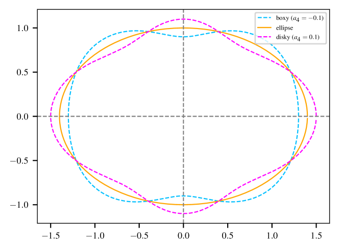
In Section 6.1 we shall investigate whether the strong lensing external shears depend on deviations from an elliptically symmetric distribution of mass. Specifically, we shall quantify the multipole deviations of two types of contour: the iso-convergence contour at $\kappa=1$ of the gNFW+MGE distributions used to create mock data, and the critical curves of both the mock and the observed galaxies. These contours are stored as a 2D array of points in polar coordinates $[\phi_{\mathrm{contour}},R_{\mathrm{contour}}]$. We calculate perpendicular deviations of each point from the true ellipse

$$R_{\mathrm{el}}(\phi)=\frac{a\sqrt{1-\epsilon^{2}}}{\sqrt{1-\epsilon^{2}\cos^{2}(\phi-\phi_{\mathrm{el}})}},$$ (16)

where $a$ is the major axis, $\phi_{\mathrm{el}}$ is the major axis orientation, and $\epsilon$ is the eccentricity (defined as $\epsilon^{2}\equiv 1-b^{2}/a^{2}$ where $b$ is the minor axis). The deviations are then parameterised using multipoles

$$\delta R_{m}(\phi;a_{m},b_{m})=\sum a_{m}\cos(m(\phi-\phi_{\mathrm{el}}))+b_{m}\sin(m(\phi-\phi_{\mathrm{el}}))\,,$$ (17)

where $m$ is the order of the multipole, and $a_{m}$ and $b_{m}$ are the magnitude of the deviations with symmetry along or at $45^{\circ}$ to the major and minor axes, respectively. We then perform a non-linear search to fit the model

$$R(\phi;a_{4},b_{4})=R_{\mathrm{el}}(\phi)+\delta R_{4}(\phi;a_{4},b_{4})$$ (18)

to the radial values of the contour. We assume uniform priors on the free parameters in the fit over a reasonable range and fit for them using the nested sampling algorithm dynesty. We assume the residual errors can be described by a Gaussian distribution and maximise the likelihood

$$\mathscr{L}(R|R_{i},\sigma)=\prod_{i}\left[\frac{1}{\sqrt{2\pi\sigma^{2}}}~{}\mathrm{exp}\left(-\frac{\left(R(\phi_{i})-R_{i}\right)^{2}}{2\sigma^{2}}\right)\right],$$ (19)

where $R_{i}$ are the radial values of the contour and $R(\phi_{i};a_{4},b_{4})$ are the model predicted values from equation (18) at each angular coordinate in the contour $\phi_{i}$. Curves with best-fit values of $a_{4}>0$ are ‘disky’; those with $a_{4}<0$ are ‘boxy’ (see Figure 1).

Figure 2: Values of the shear along the lines of sight to 39 galaxy-galaxy lenses, independently measured using strong lensing ‘external’ shear $\gamma^{\mathrm{SL}}$ and weak lensing $\gamma^{\mathrm{WL}}$. Shears are oriented such that $\gamma^{\mathrm{SL}}_{2}=0$, and rescaled to be at the same effective redshift. If strong and weak lensing shears were identical, all points would lie on the dashed lines. We instead find that external shears inferred from strong lensing are consistently larger than those measured by weak lensing, and not aligned.

5 Results

5.1 SL shears do not correlate with WL shears

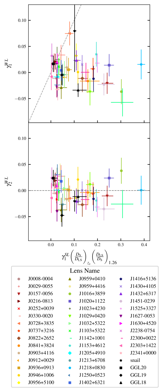
Strong lensing measurements of shear $\gamma^{\mathrm{SL}}$ (obtained as the best-fit external shear $\gamma^{\mathrm{ext}}$) typically have amplitudes up to an order of magnitude larger than weak lensing measurements $\gamma^{\mathrm{WL}}$ along the same line of sight. The mock lenses have mean best-fit $|\langle\gamma^{\mathrm{SL}}\rangle|=0.019\pm 0.002$, despite the true values all being $\gamma^{\mathrm{ext}}=0$. Our measurement using a PL+ext mass model is consistent with C22’s value $|\langle\gamma^{\mathrm{SL}}\rangle|=0.015$ using pixel-based source reconstructions. The real lenses have mean best-fit shear $|\langle\gamma^{\mathrm{SL}}\rangle|=0.098\pm 0.011$, which is much larger than both the measured weak lensing shear $|\langle\gamma^{\mathrm{WL}}\rangle|=0.028\pm 0.002$.

Strong lensing measurements of shear do not correlate with weak lensing measurements (Figure 2). To make this comparison (for the real lenses only), we first define rotated coordinate systems such that $\gamma_{1}^{\mathrm{SL}}=\gamma^{\mathrm{SL}}\geq 0$ and $\gamma_{2}^{\mathrm{SL}}=0$. Thus we need plot only three of the four components of shear. Second, we compensate for the different redshifts of the strongly lensed and weakly lensed sources by rescaling values of $\gamma_{1}^{\mathrm{SL}}$ by $(D_{\rm s}/D_{\rm ls})_{z_{s}^{\prime}=z_{s}}(D_{\rm ls}/D_{\rm s})_{z_{s}^{\prime}=1.26}$, i.e. the effective value at the redshift of the weakly lensed galaxies (see eqn 2). This scaling is exact only if the external shear is both real and dominated by neighbouring structures at the same redshift as the lens (Wong et al. 2011 found that 5/8 of the shear is from neighbouring structures). In any case, the rescaling is by a factor with mean of only 1.26 and rms 1.06, and our conclusions do not change if the rescaling is omitted or normalised to a different redshift. If strong and weak lensing measure the same quantity, we then expect $\gamma_{1}^{\mathrm{WL}}$ to correlate with $\gamma_{1}^{\mathrm{SL}}$, and $\gamma_{2}^{\mathrm{WL}}$ to scatter around zero. We find that $\langle\gamma_{2}^{\mathrm{WL}}\rangle=-0.004\pm 0.003$ is on average below zero, and its scatter (0.02) is consistent with uncertainties calculated from the distribution of weak lensing shears. The best-fit slope $\gamma_{1}^{\mathrm{WL}}=(-0.06\pm 0.04)\gamma_{1}^{\mathrm{SL}}$ actually infers a negative correlation, however this does not take into account the uncertainty on the strong lensing shears and so the uncertainty is likely underestimated. The Pearson correlation coefficient $-0.19\pm 0.22$ implies that, if there is a correlation, there is also a large amount of scatter.

There are eight lenses for which $\gamma^{\mathrm{ext}}\approx\gamma^{\mathrm{WL}}$, including two of the four lenses which reside in the outskirts of clusters (see Section 5.4 for further discussion). However, there does not appear to be anything unique about these lenses that would make the shear possible to measure in these cases.

5.2 SL shears are (suspiciously) aligned with the mass

Figure 3: Relative orientation of the strong lensing ‘external’ shear and the major axis of the lens mass, in mock (top panel) and real HST (bottom panel) data. In both cases, most of the shears are suspiciously aligned ($\phi^{\mathrm{PL+ext}}_{\mathrm{mass}}-\phi^{\mathrm{PL+ext}}_{\mathrm{ext}}\leqslant 30^{\circ}$) or anti-aligned ($\phi^{\mathrm{PL+ext}}_{\mathrm{mass}}-\phi^{\mathrm{PL+ext}}_{\mathrm{ext}}\geqslant 60^{\circ}$) with the lens mass distribution. If the $\gamma_{\mathrm{ext}}$ parameter were measuring true external perturbations, the orientations would be random. Points are coloured by the best-fit axis ratio of the lens mass distribution. Highly elliptical lenses often lead to high values of $\gamma_{\mathrm{ext}}$.

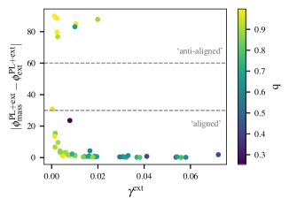
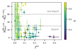
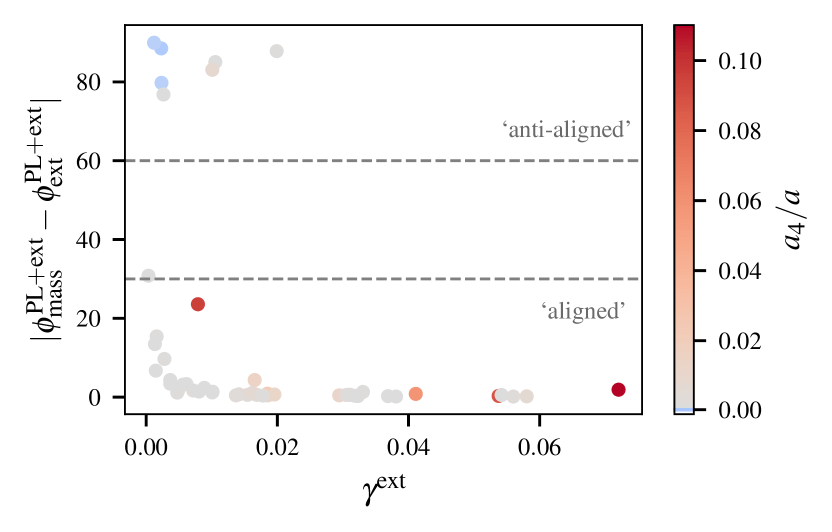
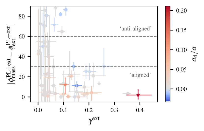
For both mock and real data, the best-fit ‘external’ shear is usually aligned with the major axis of the lens mass ($\phi^{\mathrm{PL+ext}}_{\mathrm{mass}}-\phi^{\mathrm{PL+ext}}_{\mathrm{ext}}\leqslant 30^{\circ}$) or with its minor axis ($\phi^{\mathrm{PL+ext}}_{\mathrm{mass}}-\phi^{\mathrm{PL+ext}}_{\mathrm{ext}}\geqslant 60^{\circ}$): see figure 3. If external shears were truly measuring external perturbations, their orientations would be random (modulo intrinsic alignments between the shape of a galaxy and its surrounding tidal field, but these are much smaller than our achieved measurement precision; Zhang et al., 2022). The preference for aligning with the mass distribution again suggests an ‘internal’ shear that compensates for the inability of a power law model to represent the more complex true distribution of mass. Furthermore, the highest values of $\gamma_{\mathrm{ext}}$ are also usually found in the most elliptical lenses.

In mock data, 84$\%$ of external shears are aligned with the mass distribution: their mean offset is $3^{\circ}$ with an rms scatter of $5^{\circ}$. 14$\%$ of external shears are anti-aligned with the mass distribution, with a mean of $85^{\circ}$ and scatter of $6^{\circ}$. Only one lens has a best-fit external shear that is neither aligned nor anti-aligned, but this also has the lowest shear amplitude ($\gamma_{\mathrm{ext}}=0.0003$), so the angle $\phi_{\mathrm{ext}}$ is ill-defined. The Pearson correlation coefficient between the best-fit axis ratios and external shears is $-0.63$.

Lens name SIS neighbour no neighbour $\gamma_{1}^{\textrm{WL}}$ $\gamma_{2}^{\textrm{WL}}$ $\gamma^{\textrm{WL}}$ $\phi^{\textrm{WL}}$ $\phi^{\textrm{BCG}}$ $\phi^{\textrm{neighbour}}$ $\gamma^{\textrm{ext}}$ $\phi^{\textrm{ext}}$ $q^{\textrm{PL}}$ $\phi^{\textrm{PL}}$ $\gamma^{\textrm{ext}}$ $\phi^{\textrm{ext}}$ $q^{\textrm{PL}}$ $\phi^{\textrm{PL}}$ MACS1149-GGL18 $0.13^{\textrm{+0.04}}_{\textrm{-0.02}}$ $40^{\textrm{+5}}_{\textrm{-5}}$ $0.48^{\textrm{+0.04}}_{\textrm{-0.02}}$ $147^{\textrm{+9}}_{\textrm{-8}}$ $0.24^{\textrm{+0.02}}_{\textrm{-0.02}}$ $26^{\textrm{+2}}_{\textrm{-2}}$ $0.82^{\textrm{+0.02}}_{\textrm{-0.02}}$ $174^{\textrm{+19}}_{\textrm{-22}}$ $0.01^{\textrm{+0.01}}_{\textrm{-0.01}}$ $-0.04^{\textrm{+0.01}}_{\textrm{-0.01}}$ 0.04 -40 85 95 Abell370-GGL19 $0.06^{\textrm{+0.01}}_{\textrm{-0.01}}$ $40^{\textrm{+3}}_{\textrm{-6}}$ $0.92^{\textrm{+0.01}}_{\textrm{-0.01}}$ $23^{\textrm{+1}}_{\textrm{-1}}$ $0.07^{\textrm{+0.03}}_{\textrm{-0.02}}$ $34^{\textrm{+7}}_{\textrm{-14}}$ $0.72^{\textrm{+0.03}}_{\textrm{-0.02}}$ $26^{\textrm{+5}}_{\textrm{-6}}$ $0.05^{\textrm{+0.02}}_{\textrm{-0.02}}$ $-0.01^{\textrm{+0.02}}_{\textrm{-0.02}}$ 0.05 -8 -100 35 MACS1149-GGL20 - - - - $0.01^{\textrm{+0.02}}_{\textrm{-0.01}}$ $13^{\textrm{+47}}_{\textrm{-49}}$ $0.51^{\textrm{+0.02}}_{\textrm{-0.01}}$ $106^{\textrm{+1}}_{\textrm{-2}}$ $0.01^{\textrm{+0.02}}_{\textrm{-0.02}}$ $0.04^{\textrm{+0.02}}_{\textrm{-0.02}}$ 0.04 40 -83 - RX J2129-GGL1 (snail) - - - - $0.11^{\textrm{+0.01}}_{\textrm{-0.01}}$ $35^{\textrm{+2}}_{\textrm{-2}}$ $0.93^{\textrm{+0.01}}_{\textrm{-0.01}}$ $-61^{\textrm{+10}}_{\textrm{-12}}$ $0.08^{\textrm{+0.08}}_{\textrm{-0.08}}$ $-0.02^{\textrm{+-0.02}}_{\textrm{--0.02}}$ 0.08 28 -57 -

Table 2: Summary of strong and weak lensing parameters for the 4 galaxy-galaxy lenses that reside in clusters. All angles are in degrees anticlockwise from West.

Real HST data produce a similar pattern, but with more scatter. Best-fit ‘external’ shears are aligned with the mass distribution in $68\%$ of the lenses, and anti-aligned in $20\%$. All the remaining $12\%$ have $\gamma_{\mathrm{ext}}<0.04$, so the angles $\phi^{\mathrm{PL+ext}}_{\mathrm{ext}}$ are noisy. The Pearson correlation coefficient between the best-fit axis ratios and external shears is $-0.60$. Despite the inferred external shears being an order of magnitude larger in the observations than in the mock data, the mass distributions are similarly elliptical: $\langle q\rangle=0.77\pm 0.02$ in the mocks, and $0.69\pm 0.02$ for HST data.

5.3 SL Shear Amplitudes Are Too Large

Along random lines of sight through the universe a shear amplitude of $\sim 1-3\%$ is expected (Keeton et al., 1997), even accounting for the different scales on which they are averaged (Valageas et al., 2004; Wong et al., 2011). SLACS and GALLERY strong lenses typically exist in field environments where shear amplitudes should therefore never exceed $\sim 5\%$ (Treu et al., 2009), however figure Figure: shear angle q shows the majority of measured SL shear amplitudes exceed $\sim 5\%$ and a large fraction exceed $\sim 10\%$. Therefore, even without WL data or detailed inspection of the SL mass models, the SL shear measurements alone are indicative of a non external origin.

5.4 Lenses in clusters

5.4.1 RX J2129-GGL1 (snail)

Of the galaxy-galaxy lenses in clusters the snail measures shears that agree most closely between the two methods. Notably, it measures the largest shear independent of the strong lensing method. Although this measurement was constrained by cluster scale strong lensing, Desprez et al. (2018) demonstrated that this value of shear is in agreement with that derived from weak lensing analysis of CLASH data (Figure 13 of that paper). The strong lensing external shear is anti-aligned with it’s mass distribution, although this is expected since the mass distribution is coincidentally orientated with it’s major axis pointing towards the cluster centre (Table 2).

Figure 4: What causes boxiness or diskiness? A Singular Isothermal Elliptical (SIE) mass distribution with a horizontal major axis has critical curves that are also elliptical with a horizontal major axis (orange). The critical curves are perturbed if the slope of the density profile $\gamma\neq 2$ (top left panel) or the external shear $\gamma^{\mathrm{ext}}\neq 0$ (bottom left panel). In particular, an aligned shear ($\gamma_{1}^{\mathrm{ext}}>0$) stretches the critical curves vertically (and the image horizontally); an anti-aligned shear ($\gamma_{1}^{\mathrm{ext}}<0$) does the opposite. Multipole measurements $a_{4}/a$ of the critical curve are shown as a function of slope (top right panel) and external shear (bottom right panel), where $a_{4}/a>0$ is “disky” and $a_{4}/a<0$ is “boxy”.

5.4.2 MACS1149-GGL20

The shears measured using the independent probes for MACS1149-GGL20 are also in agreement, although the shear magnitude is much lower than is measured for the snail. In fact, this is one of the few lenses that measures a lower best-fit value of shear magnitude with strong lensing $\gamma^{\mathrm{ext}}=0.01$ than it does with the weak lensing method $\gamma^{\mathrm{WL}}=0.04$. Desprez et al. (2018) found that measurements of external shear from modelling the GGL alone were underestimated compared to the shears constrained using a full scale model of the galaxy cluster. However, both of these measurements are larger than either of the shears measured in this work. The authors measure an external shear magnitude $\gamma^{\mathrm{ext}}=0.13^{+0.08}_{-0.06}$ when modelling the potential of the lens as a double Pseudo-Isothermal Elliptical profile (dPIE), significantly larger than that measured in this work $\gamma^{\mathrm{ext}}=0.01^{+0.02}_{-0.01}$. However, we measure a more elliptical mass distribution $q=0.51^{+0.02}_{-0.01}$ than was constrained by (Desprez et al., 2018) $q=0.81$. The degeneracy between shear and axis ratio may therefore explain this discrepancy. As with the snail, the mass distribution coincidentally points towards the cluster centre, therefore the anti-alignment of the external shear with the lens’ mass distribution that we infer is to be expected.

5.4.3 Abell370-GGL19

We measure a similar shear magnitude with strong lensing for Abell370-GGL19 as we do with weak lensing, but the strong lensing external shear is suspiciously orientated towards a nearby neighbour galaxy and is aligned with the mass distribution (see Table 2). We therefore repeat the fit including free parameters for a singular isothermal sphere (SIS; $\gamma=2$ and $q=1$ in equation 11) fixed at the centre of the neighbour galaxy. The results including the mass of the neighbour galaxy do not change significantly (see the SIS neighbour column of Table 2 compared to the no neighbour column), although the power-law mass distribution does become less elliptical.

5.4.4 MACS1149-GGL18

There is also a neighbour galaxy in close proximity to MACS1149-GGL18. We, therefore repeat the fit for including an SIS as was done for Abell370-GGL19. The shear is significantly overestimated as compared with weak lensing when the neighbour is not included in the fit. Including the neighbour galaxy halves the inferred strong lensing external shear, but this is still inconsistent with the weak lensing measurement. The shear is anti-aligned with the power-law mass distribution which, given that the mass distribution is not aligned with the cluster galaxy in this case, suggests the external shear may be acting internally as discussed in the previous section.

6 Analysis

6.1 External shear may compensate for boxiness/diskiness

Our measurements in Section 5 suggest that $\gamma^{\mathrm{ext}}$ mostly just compensates for the inability of a power law model to capture the complex distributions of mass (gNFW+MGE for the mocks, and likely more complex for real galaxies). This is consistent with the conclusion of Keeton et al. (1997), who inferred that the $\langle\gamma^{\mathrm{ext}}\rangle\sim 10$–$15\%$ required to fit point-source quad lenses, must reflect an inability of the lens model to capture a complex distribution of mass: perhaps misalignment between light and dark matter. Witt & Mao (1997) reached a similar conclusion, and derived an analytical prediction of the shear required by an elliptical potential to fit quad lenses.

If the external shears result from a lack of complexity in the power law model to describe the underlying distribution of mass, one can ask what type of complexity the data requires. One possible deviation from the symmetry of an elliptical power law is boxiness and diskiness (see Section 4.3). We shall now investigate whether spurious external shear could arise to compensate for boxy/disky lens galaxies.

6.1.1 External shear creates boxy/disky critical curves

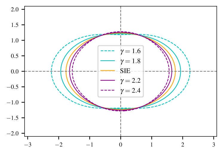
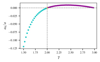
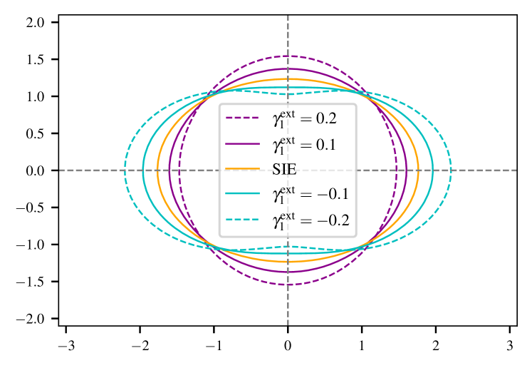
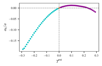
An isothermal elliptical mass distribution has an elliptical critical curve (oriented in the same direction as the mass distribution but at $90^{\circ}$ to the elongation of light from the source galaxy; Kochanek et al. 2004). However, changing the power law slope, $\gamma\neq 2$, or adding an external shear, $\gamma^{\mathrm{ext}}\neq 0$, perturbs the critical curves (left panel of Figure 4). These perturbations include significant $a_{4}/a$ moments (right panels of Figure 4), although they visually appear to be more than pure $m=4$ modes (c.f. Figure 1).

Figure 5: In mock lenses, disky ($a_{4}/a>0$) perturbations of the $\kappa=1$ isodensity contour correlate with disky perturbations of the critical curves – which can also be measured for real lenses. To better visualise the correlation, values have been transformed by $\log[a_{4}/a+0.01]$, with dashed lines indicating $a_{4}=0$. Unfortunately, the mock data do not include any lenses with significantly boxy ($a_{4}/a<0$) distributions of mass. These points come from fits with Sersic sources, so the uncertainties are not comparable to those from analyses with pixellated sources.

6.1.2 Disky critical curves come from disky mass distributions

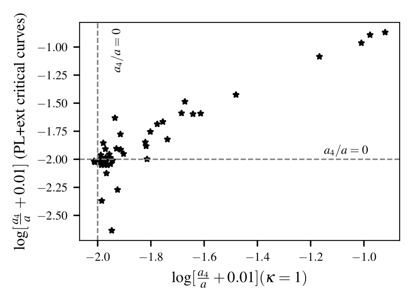
The distributions of mass in our mock lenses happen to be almost all disky. We could measure any isodensity contour, but the $\kappa$=$1$ contour will be near the most sensitive region for lens fitting. These iso-convergence contours have mean $\langle|a_{4}/a|\rangle=0.01$ and $\langle|b_{4}/a|\rangle=0.0005$. Only three lenses are boxy, but not usefully so, with very low values $\langle a_{4}/a\rangle=-0.0003$.

Critical curves of the best-fit PL+ext models to our mock data show $a_{4}/a$ moments highly correlated with those of the density contours (Figure 5). Again, $\langle|b_{4}/a|\rangle=0.0001$ is an order of magnitude lower. Studying the same mocks, C22 also noted that ‘external’ shear allowed the best-fit critical curves to better match the true critical curves. We find two systems with boxy critical curves $a_{4}/a<-0.01$. Subject to some scatter, however, we conclude that the diskiness of isodensity contours and critical curves are highly correlated.

Notably, all mock lenses whose best-fit external shear is aligned with the mass distribution have very disky critical curves (red points in Figure 6), and the three mock lenses with boxy critical curves have anti-aligned shear. Furthermore, $a_{4}$ typically increases with the external shear (Pearson correlation coefficient 0.45) and with the axis ratio of the lens mass (Pearson correlation coefficient $-0.73$). This may be tentative evidence that (some of) the dichotomy of aligned and anti-aligned shears may be caused by diskiness or boxiness.

Figure 6: For mock lenses that were simulated without external shear. Angle between the best-fit values of external shear and the major axis of the lens mass distribution, $|\phi^{\mathrm{PL+ext}}_{\mathrm{mass}}-\phi^{\mathrm{PL+ext}}_{\mathrm{ext}}|$ in degrees, as a function of the amplitude of the best-fit external shear, $\gamma_{\mathrm{ext}}$. Points are coloured by the magnitude of the inferred critical curves deviation from elliptical symmetry $a_{4}/a$, values of $a_{4}/a<0$ correspond to boxy critical curves and $a_{4}/a>0$ to disky ones. Note the red and blue colour points are orders of magnitude different, the blue range reaches a maximum of 0.001.

Figure 7: Same as for Figure 6 but for the observed SLACS and GALLERY lenses. The inferred external shears have a similar distribution of aligned and anti-aligned shears as the mock data sample, indicating they too may be acting internally. Note the increase in the scale of shear magnitude $\gamma_{\mathrm{ext}}$ and elliptical deviations $a_{4}/a$ compared to the mock data sample.

6.1.3 Does boxiness/diskiness cause ‘external’ shear?

Scatter in real data is larger than in the mocks. However, for SLACS and GALLERY lenses, the best-fit critical curves have mean $\langle|a_{4}/a|\rangle=0.016$, similar to the mocks. Most ($79\%$ of) lenses with best-fit ‘external’ shear that is aligned with the mass distribution have disky critical curves; and most ($70\%$) with anti-aligned shear have boxy critical curves (Figure 7). Moreover, lenses with the largest amplitude of external shear also have critical curves with the largest deviations from elliptical (Pearson correlation coefficient of 0.48 with $a_{4}$ and 0.65 with $b_{4}$).

This provides tentative evidence that ‘external’ shear in typical lensing analyses is really caused by the inability of parametric mass models to capture the complex distribution of mass in a lens. A substantial portion of that complexity may be diskiness or boxiness of the mass distribution. This creates diskiness or boxiness in the critical curves (Section 6.1.2), which leads to a spurious external shear (Section 6.1.1). We have not been able to quantify the relative contributions to external shear from true shear, diskiness/boxiness, or other sources.

6.1.4 More things probably cause ‘external’ shear too

There are likely more sources of complexity in real mass distributions, which cause (or are compensated by) external shear. These confounding factors would explain the looser correlations and larger scatter than in the mocks. Just the observation that real lenses have external shears with amplitudes six times greater than mocks implies that their distribution of mass deviates more from a power law.

We speculate that the isodensity contours of a lens might be twisted (misaligned as a function of radius), like their isophotoes. Indeed, the critical curves of SLACS and GALLERY lenses have a handedness, with $\langle|b_{4}/a|\rangle=0.012$ two orders of magnitude larger than the mocks. If the critical curves do tell us something about the distribution of mass, this may indicate twisted isodensity contours. Twisting is also suggested by the inconsistently measured position angle when real data are fitted with and without external shear (see Figure 9); this is not present in the mocks. Van de Vyvere et al. (2022) also found that twists in the underlying mass distribution are typically absorbed by changes in orientation of the mass distribution and shear in a PL+ext model. The maximum amplitude of external shear that can be attributed to these twists is around $5\%$ to $8\%$ (see Figures B3 and B4 of Van de Vyvere et al., 2022), but lower values are more common for most of their mock lenses. Given many of our strong lenses have shear amplitudes above $\sim 10\%$, twists alone cannot explain all of the SL shears measured.

6.2 External shear biases other SL model parameters

Since best-fit values of ‘external’ shear may not (entirely) represent the physical quantity they are imagined to, we now test which other parameters in the mass model are biased by their inclusion, and which are still robustly measured. As an extreme alternative, we repeat all measurements but fix $\gamma^{\mathrm{ext}}_{1}=\gamma^{\mathrm{ext}}_{2}=0$ when we refit the mass distribution.

6.2.1 Mock lenses

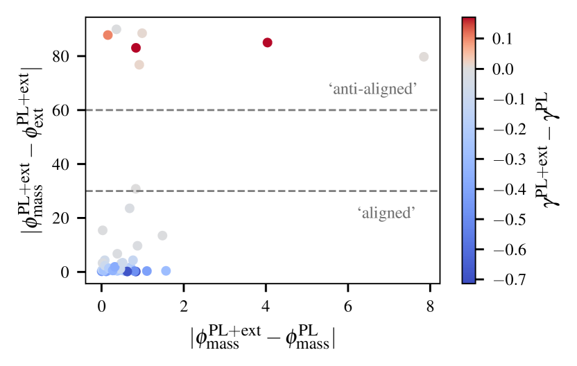
The orientation of the mass distribution is robustly measured, with mean difference $\langle|\phi^{\mathrm{PL+ext}}_{\mathrm{mass}}-\phi^{\mathrm{PL}}_{\mathrm{mass}}|\rangle\sim 1^{\circ}$ and only $\sim 1^{\circ}$ of scatter when shear is excluded (figure 8). The axis ratio is also hardly changed, with $\langle q^{\mathrm{PL+ext}}-q^{\mathrm{PL}}\rangle=0.01\pm 0.05$. These values are so robust because all the MGE components share a common axis, which is therefore well-defined.

However, the Einstein radii and slopes of the power-law mass model are systematically biased, by an amount that depends on the relative orientation of the shear and the mass (Einstein radii and power-law slopes are known to be degenerate parameters: see e.g. figure 5 of E22). For lenses whose shears were aligned with the mass distribution, removing $\gamma^{\mathrm{ext}}$ increases the mean best-fit power-law slope by $0.20\%\pm 0.04$ (blue points in figure 8; their mean best-fit Einstein radii decrease by $0.2\pm 0.03\%$). For lenses whose shears were anti-aligned, the power-law slopes decrease by $0.07\pm 0.03$ (red points in figure 8; their mean best-fit Einstein radii increase by $0.08\pm 0.04$). Across the entire sample, Einstein radii had been correctly measured when including $\gamma^{\mathrm{ext}}$ (within $0.05\pm 0.17\%$; Cao et al., 2022), but are systematically underestimated by $0.2\%\pm 0.05\%$ if shear is excluded.

Our measurements might be caused by a bias described by Kochanek (2021) in the radial structure of a lens, when a model has too few azimuthal degrees of freedom. Kochanek provides the example of fitting a power-law model to a lens whose ellipticty increases with radius: the density slope is forced to spuriously shallow values to balance the shear inside the Einstein radius relative to the shear outside it. Furthermore, Van de Vyvere et al. (2022) found that decreasing ellipticity outside the Einstein radius spuriously increases $\gamma^{\mathrm{ext}}$ for a power-law model, while ellipticity gradients inside or at the Einstein radius mainly bias the power-law slope. In our mocks, the distribution of mass has an ellipticity which varies as a function of radius. We attempted to find a correlation of the measured shear properties (e.g. position angle) with the ellipticity variation of the mock mass distributions. However, we were unable to detect a statistically significant correlation. We interpret this as the measured shear depending on other properties of each lens (e.g. where the lensed source’s arcs appear in the image-plane). A more detailed investigation is beyond the scope of this work.

Figure 8: For mock lenses that were simulated without external shear. Angle between the best-fit external shear and the major axis of the lens mass distribution, $|\phi^{\mathrm{PL+ext}}_{\mathrm{mass}}-\phi^{\mathrm{PL+ext}}_{\mathrm{ext}}|$ in degrees, as a function of the change in orientation of the major axis when fitting with and without an external shear, $|\phi^{\mathrm{PL+ext}}_{\mathrm{mass}}-\phi^{\mathrm{PL}}_{\mathrm{mass}}|$. Points are coloured by the difference in power-law slope inferred between the models fitted with and without an external shear ($\gamma^{\mathrm{PL+ext}}-\gamma^{\mathrm{PL}}$). Systems with best-fit shear aligned to the mass systematically decrease in power-law slope when the external shear is removed from the model (blue points). Anti-aligned shears exhibit the opposite behaviour (red points).

6.2.2 Real lenses

Figure 9: Orientation angle offset of the external shear from the PL+ext mass distribution ($\phi^{\mathrm{PL+ext}}_{\mathrm{mass}}-\phi^{\mathrm{PL+ext}}_{\mathrm{ext}}$) as a function of the difference in orientation angle when the mass distribution is fitted with and without an external shear ($\phi^{\mathrm{PL+ext}}_{\mathrm{mass}}-\phi^{\mathrm{PL}}_{\mathrm{mass}}$) for the observed SLACS and GALLERY samples. Scatter points are coloured by the difference in axis ratio of the models fitted with a PL+ext and a PL ($q^{\mathrm{PL+ext}}-q^{\mathrm{PL}}$).

Figure 10: Histograms of the difference between inferred PL mass distribution model parameters with external shear as free parameters, minus those without shear, for the observed (pink) and mock data samples (orange). From left to right panels the parameters are: fractional Einstein radius, logarithmic slope of density profile, axis ratio of mass distribution, and radial distance of the centre of the mass distribution, in arcseconds.

Figure 11: Fractional difference between Einstein radii inferred for models with and without the free parameters for external shear, as a function of the external shear amplitude.

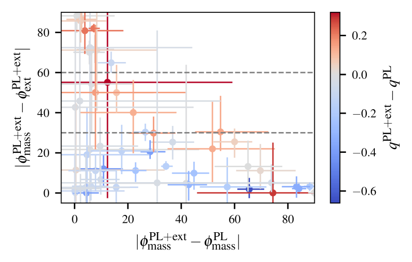
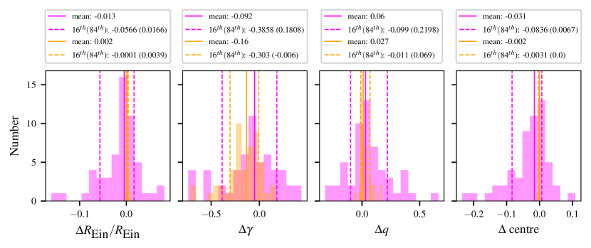
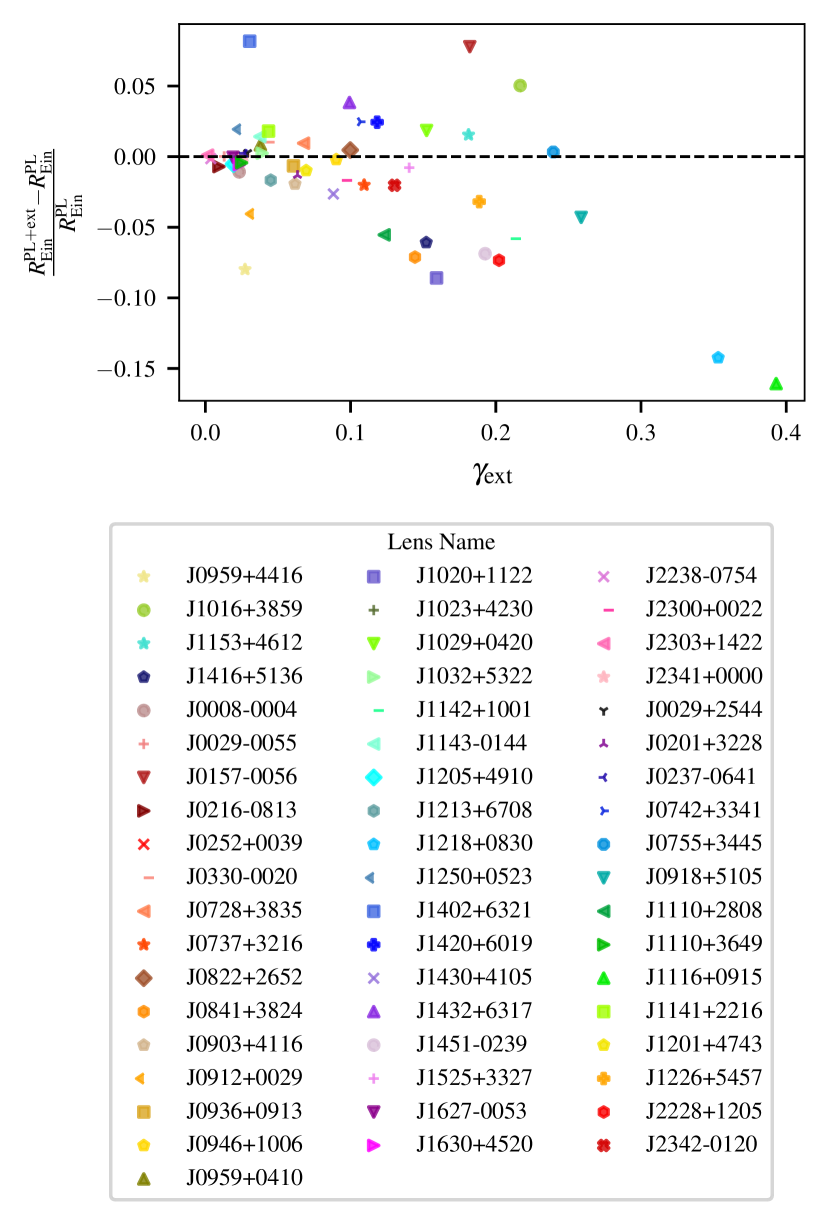
For SLACS and GALLERY lenses, the orientation of the mass distribution changes considerably when external shear is removed, with $\langle|\phi^{\mathrm{PL+ext}}_{\mathrm{mass}}-\phi^{\mathrm{PL}}_{\mathrm{mass}}|\rangle\sim 27^{\circ}$ and $\sim 27^{\circ}$ scatter (figure 9; note the different scale on the horizontal axis to figure 8). The best-fit axis ratio (indicated by colour in figure 9) also increases by $0.18\pm 0.016$ for aligned systems, which become more spherical; decreases by $0.08\pm 0.10$ for anti-aligned systems, which become more elliptical; and is inconsistent for the rest, with mean change $\langle q^{\mathrm{PL+ext}}-q^{\mathrm{PL}}\rangle=-0.02\pm 0.04$.

Neither the Einstein radii nor slopes of the power-law mass model are systematically biased when external shear is removed. We find $\langle\Delta R_{\mathrm{Ein}}/R_{\mathrm{Ein}}\rangle=-0.013^{+0.030}_{-0.043}$, where $\Delta R_{\mathrm{Ein}}\equiv R_{\mathrm{Ein}}^{\mathrm{PL+ext}}-R_{\mathrm{Ein}}^{\mathrm{PL}}$. However, the best fit values scatter about the same mean, such that ${\langle\Delta R_{\mathrm{E}in}^{2}/R_{\mathrm{E}in}\rangle}=0.045^{2}$, which is two orders of magnitude larger than the equivalent $0.0003^{2}$ value for the mocks (figure 10). Furthermore, the scatter increases with increasing external shear magnitude (figure 11).

The best-fit centre of the mass distribution moves on average by $-0.031\pm 0.061\arcsec$ when external shear parameters are introduced, and on average remains $0.05\pm 0.06\arcsec$ from the centre of light. With or without shear, this offset is an order of magnitude greater than in the mock data.

We suspect this indicates that the distribution of mass in real galaxies is more complex than that in the mocks: for example with multiple components that are rotationally offset from one another and no single, well-defined axis of ellipticity.

7 Interpretation

7.1 Strong lensing external shears are not measuring shear

We find that external shear, as measured by galaxy-galaxy strong lensing, does not correlate well with the true shear along a line-of-sight (as measured independently by weak lensing; Section 5.1 and Figure 2). Best-fit values of external shear are also frequently several times higher than that along typical lines of sight through the Universe, so only a small fraction of it could be due to true shear. Rather, external shear tends to align with either the major axis or minor axis of the lens mass distribution (Section  5.2). It appears to be compensating for the inflexibility of typical mass models (here an elliptical power-law) to represent the complex distributions of mass. A substantial portion of that complexity appears to be diskiness and boxiness (Section 6.1), especially in mock data. In real data, isophotal twists, elliptical gradients, and offsets in the centres and alignments of dark and stellar matter all increase uncertainty on model parameters. These have all been seen in the stellar mass of SLACS lenses (Nightingale et al., 2019). We have not been able to quantify how much each source contributes to the scatter or bias in a real measurement of external shear.

Hogg et al. (2022) suggest a different, ‘minimal line-of-sight’ way of parameterising the shear that is less degenerate with lens model parameters, but this is still subject to biases in the shear parameters when simplifying assumptions are made for the lens model. For complex distributions of lens mass, the false inference of external shear will pose a challenge for efforts to use strong lensing to measure cosmic shear (e.g. Birrer et al., 2017; Fleury et al., 2021).

7.2 Implications for strong lensing science goals

Including external shear alters the best-fit values of other parameters (Section 6.2). In mock data, some parameters do move closer to the known truth: the mean error in power law slopes is $-0.02\pm 0.10$ with shear, or $-0.14\pm 0.20$ without it. A $\sim 0.2\%$ bias in Einstein radii also disappears with shear. However, the shear is not physically real and, contributing zero convergence, does not correspond to a physically meaningful distribution of mass. For studies that rely on accurate reconstructions of the mass distribution (e.g. galaxy evolution, dark matter physics, and the Hubble constant), this degeneracy with key parameters will eventually limit statistical precision. For example, a key result of the SLACS survey was that elliptical galaxies have isothermal ($\gamma$=$2$) mass profiles (Gavazzi et al., 2007; Vegetti & Koopmans, 2009; Auger et al., 2010). Including external shear, measured $\langle\gamma\rangle=2.0756^{+0.023}_{-0.024}$ for SLACS galaxies; here we measure $\langle\gamma\rangle=2.0159=^{+0.027}_{-0.032}$ (Figure 10), highlighting the systematic uncertainty that will remain fixed even if the sample size increases. Furthermore, a PL+ext model leaves false detections of subhalos in a mock disky galaxy (He et al., 2023) or real HST data (Nightingale et al., 2023a).

The Hubble constant $H_{0}$ can be measured from the time delay between multiple images (Suyu et al., 2017; Wong et al., 2019; Birrer et al., 2019). However, assuming specific functional forms for the mass model can artificially break the mass-sheet transformation. Our tests on mock data (Section 6.2.1) demonstrate a coupling, predicted by Kochanek (2021), between angular and radial structure. Oversimple models bias the slope, and hence bias $H_{0}$. C22 estimated $\sim$9% bias in $H_{0}$ when using a PL+ext model to interpret time delays generated from gNFW+MGE lenses. The angular degrees of freedom added by ‘external’ shear are insufficient to compensate for even this complexity. Given that our analysis of SLACS and GALLERY lenses indicate even more angular degrees of freedom, such as twists in the mass distribution, biases for real lensing systems will likely be closer to the 20–50% suggested by other studies (Schneider & Sluse, 2013; Xu et al., 2016; Kochanek, 2020; Gomer & Williams, 2018, 2020, 2021). More flexible models, such as adding an internal mass sheet to the PL+ext model which is contstrained via stellar dynamics, have been introduced to mitigate these systematics.

Combining $H_{0}$ measurements from a large population of lenses might average away individual biases up to $10\mathrm{kms}^{-1}\mathrm{Mpc}^{-1}$, on the assumption that boxy and disky mass distributions are equally well represented (Van de Vyvere et al., 2022). However, the diskiness of the mass distribution correlates with the diskiness of the (observable) PL+ext critical curves (Section 6.1.2), and our observationally-selected sample contains an overpopulation of 71% disky galaxies (Section 6.1.3). More flexible mass models (e.g. a PL with an internal mass sheet) have also been introduced (Birrer et al., 2020), which infer unbiased $H_{0}$ values on mock lens samples (Ding et al., 2021). Moreover, Van De Vyvere et al. (2022) did not investigate the effect of $b_{4}$ ‘twisting’ perturbations (Section 6.1.4) or mis-centering (Section 6.2.2), both of which we observe in the critical curves of real galaxies, and whose effects may not average away. For example, the centre of mass in the H0LiCOW model of lens WFI 2033-4723 is offset from the centre of light by $\sim$10$\times$ astrometric uncertainty (Suyu et al., 2010; Barrera et al., 2021), and a similar offset in iPTF16geu increases asymmetry (Diego et al., 2022). Such offsets are unphysical (Schaller et al., 2015), so it is not clear that complexities in the mass distributions of real lenses can be safely ignored by averaging over a population.

7.3 Future work: more complex mass models are needed

External shear does not appear to be sufficient as (the sole) parameter to encode all the complexity in real lenses. Although Einstein radii are expected to be ‘model independent’ within ${\sim}2\%$ uncertainty Bolton et al. (2008b); Sonnenfeld et al. (2013), the 4.5% RMS fractional difference we measure with and without shear, suggests an unknown unknown. A single power-law model leads to mass discrepancies with stellar dynamics (Etherington et al., 2023), and spurious false-positives in searches for dark matter subhalos (Nightingale et al., 2023a). Further work (e.g. Cao et al., 2022; Van De Vyvere et al., 2020; Van de Vyvere et al., 2022) to understand the types of asymmetries that must be accounted for in the lens modelling, and the possibility of constraining such models, will be invaluable.

What parametric forms allow sufficient complexity — in a minimum number of parameters that need to be constrained? Even our gNFW+MGE mocks still do not capture the full complexity of real lenses, but their MGEs were forced to be aligned. Perhaps the model could have both $a_{4}$ and $b_{4}$ perturbations, varying as a function of radius. Cluster-scale models frequently use a soft core inside some scale radius, and (Limousin et al., 2022) add B-spline functions. The number of free parameters must be balanced with the information available: pixellated mass models are generally underconstrained (and although they might be able to fit observations without external shear; Valls-Gabaud et al. 2006, some line-of-sight shear is expected for galaxy-scale lenses). To instead increase the available information, the total mass could be decomposed into dark matter and stellar components, with the latter informed by the lens light (which is otherwise a nuisance). Whatever the parametric form, the azimuthal degrees of freedom must be defined carefully to avoid the bias described by Kochanek (2021) on the inference of the radial mass distribution. We suggest more studies (e.g. Van De Vyvere et al., 2020; Van de Vyvere et al., 2022, C22), embedded deeply in each specific science case, to quantify the impact of simplifying assumptions.

A silver lining is that the sensitivity of galaxy-galaxy strong lensing data may be a new opportunity. Both our results and those of Van De Vyvere et al. (2022) suggest that it might be possible to measure the diskiness or boxiness of galaxies’ dark matter halos. Our results are even more optimistic: if measurable multipole perturbations in critical curves traces those in the distributions of both mass and light, then one could study the dark morphology of galaxies at high redshift with relative ease.

Data Availability

Text files and images of every model-fit performed in this work are available at https://zenodo.org/record/6104823. Full dynesty chains of every fit are available upon request.

Software Citations

This work uses the following software packages:

• Astropy (Astropy Collaboration, 2013; Price-Whelan et al., 2018)

• Corner.py (Foreman-Mackey, 2016)

• Dynesty (Speagle, 2020)

• Matplotlib (Hunter, 2007)

• Numba (Lam et al., 2015)

• NumPy (van der Walt et al., 2011)

• PyAutoFit (Nightingale et al., 2021a)

• PyAutoGalaxy (Nightingale et al., 2023b)

• PyAutoLens (Nightingale & Dye, 2015; Nightingale et al., 2018, 2021b)

• Python (Van Rossum & Drake, 2009)

• Scikit-image (Van der Walt et al., 2014)

• Scikit-learn (Pedregosa et al., 2011)

• Scipy (Virtanen et al., 2020)

• SQLite (Hipp, 2020)

Appendix A Systematic Tests of Shear Measurement

Figure 12: Best-fit external shear amplitude $\gamma^{\rm ext}$ and position angle $\phi^{\rm ext}$ for every lens in the sample. Shear values are shown for the lens models presented in the main paper which do not include nearby line-of-sight galaxies and for an additional set of lens model fitted, which include up to two nearby galaxies as SISs. Error bars are at 1$\sigma$ confidence intervals. The lens light subtraction and source analysis of every fit are the same, enabling a direct comparison of how the shear values change when nearby galaxies are included in the mass model. The inferred $\gamma^{\rm ext}$ and $\phi^{\rm ext}$ values are consistent with one another in the vast majority of lenses, irrespective of whether line-of-sight galaxies are included. In the right figure, models with $\gamma^{\rm ext}<0.05$ are shown in black, illustrating that the measured values are only inconsistent for low shear lenses. Lensing due to nearby galaxies therefore is not responsible for the large shears which align with the lens mass model found in the main paper.

Figure 13: Best-fit external shear amplitude $\gamma^{\rm ext}$ and position angle $\phi^{\rm ext}$ for every lens in the sample. Shear values are shown for the lens models presented in the main paper which use a Voronoi mesh with luminosity based regularization and for an additional set of model fitted, which use a Delaunay mesh with interpolation regularization (see appendix A of Nightingale et al. 2023c). Error bars are at 1$\sigma$ confidence intervals. In the right figure, models with $\gamma^{\rm ext}<0.05$ are shown in black, illustrating that the measured values are only inconsistent for low shear lenses. The inferred $\gamma^{\rm ext}$ and $\phi^{\rm ext}$ values are consistent with one another in the vast majority of lenses, irrespective of the source model. The source analysis therefore does not impact our main conclusions.

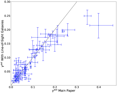
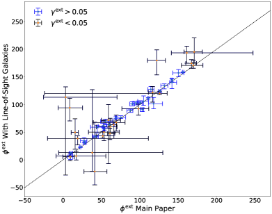
Real external shear is caused by galaxies or clusters of galaxies adjacent to the line of sight (Wong et al., 2011). It is possible that individual galaxies impart a localised external shear that is unmeasurable by weak lensing, which averages over large spatial scales. Here we repeat our analysis of every SLACS and GALLERY lens, but including adjacent galaxies in the mass model. Crucially, we use identical lens light subtraction and source pixellization, so we can directly compare the inferred shears.

We select which adjacent galaxies to include subjectively, based on their proximity and size. To implement this, we extend this study’s $LP^{\rm 1}$ pipeline (Etherington et al., 2023) with a GUI where we look at $10\arcsec$ cut-outs of each lens and click on up to two galaxies. These are added to the mass model as spherical isothermal spheres (SIS, an SIE with $q=1$), fixed to the centre of their brightest pixel and the same redshift as the main lens. Their Einstein radius $\theta^{\rm mass}_{\rm E}$ is given a flat prior from $0.0\arcsec$ to $0.5\arcsec$ and fitted with all other parameters. $\theta^{\rm mass}_{\rm E}=0.5\arcsec$ corresponds to a mass far greater than that suggested by each galaxy’s luminosity. It is an intentional choice not to use more informative priors, so that we can investigate how line-of-sight galaxies change the shear inference with maximal freedom.

Adjacent galaxies do not significantly change the inferred external shear (Figure 12). For almost every lens, the best-fit external shear for models with and without adjacent galaxies remains consistent. Large amplitudes of external shear are still preferred for many lenses, and their position angles still show the same alignment with the mass model position angles (not shown). The very largest external shears $\gamma_{\mathrm{ext}}\gtrsim 0.3$ may be reduced, with a small statistical sample but with the two highest ($\sim$$0.40$ and $\sim$$0.36$) becoming $\sim$$0.21$ and $\sim$$0.24$ after accounting for adjacent galaxies. Such values remain physically infeasible. These results confirm that line-of-sight galaxies cannot explain the conclusions of this paper.

Appendix B Sensitivity to Source Model

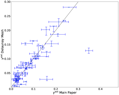
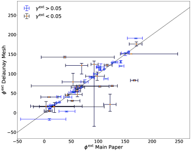
We investigate whether the shear measurements presented in the main paper depend on assumptions related to the source model. In the main paper, we followed Etherington et al. (2023) in reconstructing the source using a Voronoi pixel mesh and a regularization scheme that adapted to the unlensed source luminosity (see Nightingale et al., 2018). As an alternative, here we model the same lenses using a Delaunay pixel mesh and the interpolation-based regularization scheme described in appendix A of Nightingale et al. (2023a).

The best-fit external shear with this alternative source-plane pixellization has amplitude and angle that is consistent with those in the main paper, for nearly every lens (see Figure 13). Our main conclusions are thus unaffected by even substantial changes in source reconstruction.

References

- Ade et al. (2016) Ade P. A., et al., 2016, Astronomy and Astrophysics, 594
- Amorisco et al. (2022) Amorisco N. C., et al., 2022, Monthly Notices of the Royal Astronomical Society, 510, 2464
- Astropy Collaboration (2013) Astropy Collaboration 2013, A&A, 558, A33
- Auger et al. (2010) Auger M. W., Treu T., Bolton A. S., Gavazzi R., Koopmans L. V., Marshall P. J., Moustakas L. A., Burles S., 2010, Astrophysical Journal, 724, 511
- Barrera et al. (2021) Barrera B., Williams L. L. R., Coles J. P., Denzel P., 2021, The Open Journal of Astrophysics, 4, 12
- Bertin & Arnouts (1996) Bertin E., Arnouts S., 1996, Astron. Astrophys. Suppl. Ser., 117, 393
- Birrer et al. (2017) Birrer S., Welschen C., Amara A., Refregier A., 2017, Journal of Cosmology and Astroparticle Physics, 2017
- Birrer et al. (2019) Birrer S., et al., 2019, Monthly Notices of the Royal Astronomical Society, 484, 4726
- Birrer et al. (2020) Birrer S., et al., 2020, Astronomy & Astrophysics, 1
- Bolton et al. (2008a) Bolton A. S., Burles S., Koopmans L. V. E., Treu T., Gavazzi R., Moustakas L. A., Wayth R., Schlegel D. J., 2008a, The Astrophysical Journal
- Bolton et al. (2008b) Bolton A. S., Treu T., Koopmans L. V. E., Gavazzi R., Moustakas L. A., Burles S., Schlegel D. J., Wayth R., 2008b, The Astrophysical Journal, 684, 248
- Bolton et al. (2012) Bolton A. S., et al., 2012, Astrophysical Journal, 757
- Cao et al. (2022) Cao X., et al., 2022, Research in Astronomy and Astrophysics, 22
- Cappellari (2002) Cappellari M., 2002, Monthly Notices of the Royal Astronomical Society, 333, 400
- Cappellari et al. (2013) Cappellari M., et al., 2013, Monthly Notices of the Royal Astronomical Society, 432, 1709
- Despali et al. (2019) Despali G., Lovell M., Vegetti S., Crain R. A., Oppenheimer B. D., 2019, Monthly Notices of the Royal Astronomical Society, 17, 1
- Desprez et al. (2018) Desprez G., Richard J., Jauzac M., Martinez J., Siana B., Clément B., 2018, MNRAS, 479, 2630
- Diego et al. (2022) Diego J. M., Bernstein G., Chen W., Goobar A., Johansson J. P., Kelly P. L., Mörtsell E., Nightingale J. W., 2022, A&A, 662, A34
- Ding et al. (2021) Ding X., et al., 2021, Monthly Notices of the Royal Astronomical Society, 503, 1096
- Etherington et al. (2022) Etherington A., et al., 2022, MNRAS, 517, 3275
- Etherington et al. (2023) Etherington A., et al., 2023, MNRAS, 521, 6005
- Faure et al. (2008) Faure C., et al., 2008, ApJS, 176, 19
- Fleury et al. (2021) Fleury P., Larena J., Uzan J.-P., 2021, JCAP, 2021, 024
- Foreman-Mackey (2016) Foreman-Mackey D., 2016, The J. Open Source Softw., 1, 24
- Gavazzi et al. (2007) Gavazzi R., Treu T., Rhodes J. D., Koopmans L. V. E., Bolton A. S., Burles S., Massey R. J., Moustakas L. A., 2007, ApJ, 667, 176
- Gomer & Williams (2018) Gomer M. R., Williams L. L. R., 2018, MNRAS, 475, 1987
- Gomer & Williams (2020) Gomer M., Williams L. L. R., 2020, JCAP, 2020, 045
- Gomer & Williams (2021) Gomer M. R., Williams L. L. R., 2021, MNRAS, 504, 1340
- Graham & Driver (2005) Graham A. W., Driver S. P., 2005, Publications of the Astronomical Society of Australia, 22, 118
- Harvey (2020) Harvey D., 2020, Monthly Notices of the Royal Astronomical Society, 498, 2871
- Harvey et al. (2019) Harvey D., Tam S.-I., Jauzac M., Massey R., Rhodes J., 2019, arXiv e-prints, p. arXiv:1911.06333
- He et al. (2022a) He Q., et al., 2022a, MNRAS, 511, 3046
- He et al. (2022b) He Q., et al., 2022b, MNRAS, 512, 5862
- He et al. (2023) He Q., et al., 2023, MNRAS, 518, 220
- Hezaveh et al. (2016) Hezaveh Y. D., et al., 2016, The Astrophysical Journal, 823, 37
- Hilbert et al. (2007) Hilbert S., White S. D. M., Hartlap J., Schneider P., 2007, MNRAS, 382, 121
- Hipp (2020) Hipp R. D., 2020, SQLite, https://www.sqlite.org/index.html
- Hogg et al. (2022) Hogg N. B., Fleury P., Larena J., Martinelli M., 2022, 19, 1
- Hunter (2007) Hunter J. D., 2007, Comput Sci Eng, 9, 90
- Keeton et al. (1997) Keeton C. R., Kochanek C. S., Seljak U., 1997, The Astrophysical Journal, 482, 604
- Kilbinger (2015) Kilbinger M., 2015, Reports on Progress in Physics, 78
- Kochanek (2020) Kochanek C. S., 2020, MNRAS, 493, 1725
- Kochanek (2021) Kochanek C. S., 2021, MNRAS, 501, 5021
- Kochanek et al. (2004) Kochanek C., Schneider P., Wambsganss J., 2004, Part 2 of Gravitational Lensing: Strong, Weak & Micro, Proceedings of the 33rd Saas-Fee Advanced Course, https://arxiv.org/abs/astro-ph/0407232
- Koopmans et al. (2009) Koopmans L. V., et al., 2009, Astrophysical Journal, 703
- Kuhn et al. (2020) Kuhn F. A., Bruderer C., Birrer S., Amara A., Réfrégier A., 2020, pp 0–26
- Lam et al. (2015) Lam S. K., Pitrou A., Seibert S., 2015, Proceedings of the Second Workshop on the LLVM Compiler Infrastructure in HPC - LLVM ’15, pp 1–6
- Leauthaud et al. (2007) Leauthaud A., et al., 2007, The Astrophysical Journal Supplement Series, 172, 219
- Li et al. (2016) Li R., Frenk C. S., Cole S., Gao L., Bose S., Hellwing W. A., 2016, Monthly Notices of the Royal Astronomical Society, 460, 363
- Li et al. (2017) Li R., Frenk C. S., Cole S., Wang Q., Gao L., 2017, Monthly Notices of the Royal Astronomical Society, 468, 1426
- Li et al. (2019) Li R., et al., 2019, Monthly Notices of the Royal Astronomical Society, 490, 2124
- Limousin et al. (2022) Limousin M., Beauchesne B., Jullo E., 2022, A&A, 664, A90
- Massey et al. (2007) Massey R., et al., 2007, ApJS, 172, 239
- Massey et al. (2010) Massey R., Kitching T., Richard J., 2010, Reports on Progress in Physics, 73
- Narayan & Bartelmann (1996) Narayan R., Bartelmann M., 1996, arXiv e-prints, pp astro–ph/9606001
- Natarajan & Springel (2004) Natarajan P., Springel V., 2004, ApJ, 617, L13
- Navarro et al. (1997) Navarro J. F., Frenk C. S., White S. D. M., 1997, ApJ, 490, 493
- Nightingale & Dye (2015) Nightingale J. W., Dye S., 2015, Monthly Notices of the Royal Astronomical Society, 452, 2940
- Nightingale et al. (2018) Nightingale J., Dye S., Massey R., 2018, Monthly Notices of the Royal Astronomical Society, 47, 1
- Nightingale et al. (2019) Nightingale J. W., Massey R. J., Harvey D. R., Cooper A. P., Etherington A., Tam S.-I., Hayes R. G., 2019, Monthly Notices of the Royal Astronomical Society
- Nightingale et al. (2021a) Nightingale J. W., Hayes R. G., Griffiths M., 2021a, J. Open Source Softw., 6, 2550
- Nightingale et al. (2021b) Nightingale J., et al., 2021b, Journal of Open Source Software, 6, 2825
- Nightingale et al. (2023a) Nightingale J. W., et al., 2023a, arXiv e-prints, p. arXiv:2209.10566
- Nightingale et al. (2023b) Nightingale J. W., et al., 2023b, J. Open Source Softw., 8, 4475
- Nightingale et al. (2023c) Nightingale J. W., et al., 2023c, MNRAS, 521, 3298
- Oldham & Auger (2018) Oldham L. J., Auger M. W., 2018, Monthly Notices of the Royal Astronomical Society, 476, 133
- Pedregosa et al. (2011) Pedregosa F., et al., 2011, Journal of Machine Learning Research, 12, 2825
- Price-Whelan et al. (2018) Price-Whelan A. M., et al., 2018, AJ, 156, 123
- Rhodes et al. (2000) Rhodes J., Refregier A., Groth E. J., 2000, The Astrophysical Journal, 536, 79
- Ritondale et al. (2019) Ritondale E., Vegetti S., Despali G., Auger M. W., Koopmans L. V., McKean J. P., 2019, Monthly Notices of the Royal Astronomical Society, 485, 2179
- Robertson et al. (2020) Robertson A., Smith G. P., Massey R., Eke V., Jauzac M., Bianconi M., Ryczanowski D., 2020, MNRAS, 495, 3727
- Schaller et al. (2015) Schaller M., Robertson A., Massey R., Bower R. G., Eke V. R., 2015, MNRAS, 453, L58
- Schneider & Sluse (2013) Schneider P., Sluse D., 2013, Astronomy and Astrophysics, 559, 1
- Shu et al. (2015) Shu Y., et al., 2015, Astrophysical Journal, 803, 1
- Shu et al. (2016a) Shu Y., Bolton A. S., Moustakas L. A., Stern D., Dey A., Brownstein J. R., Burles S., Spinrad H., 2016a, The Astrophysical Journal, 820, 43
- Shu et al. (2016b) Shu Y., et al., 2016b, The Astrophysical Journal, 824, 86
- Smail et al. (1994) Smail I., Ellis R. S., Fitchett M. J., 1994, MNRAS, 270, 245
- Sonnenfeld et al. (2012) Sonnenfeld A., Treu T., Gavazzi R., Marshall P. J., Auger M. W., Suyu S. H., Koopmans L. V., Bolton A. S., 2012, Astrophysical Journal, 752
- Sonnenfeld et al. (2013) Sonnenfeld A., Treu T., Gavazzi R., Suyu S. H., Marshall P. J., Auger M. W., Nipoti C., 2013, Astrophysical Journal, 777
- Speagle (2020) Speagle J. S., 2020, MNRAS, 493, 3132
- Suyu (2012) Suyu S. H., 2012, Monthly Notices of the Royal Astronomical Society, 426, 868
- Suyu et al. (2010) Suyu S. H., Marshall P. J., Auger M. W., Hilbert S., Blandford R. D., Koopmans L. V. E., Fassnacht C. D., Treu T., 2010, ApJ, 711, 201
- Suyu et al. (2017) Suyu S. H., et al., 2017, Monthly Notices of the Royal Astronomical Society, 468, 2590
- Tam et al. (2020) Tam S. I., et al., 2020, Monthly Notices of the Royal Astronomical Society, 496, 4032
- Treu et al. (2009) Treu T., Gavazzi R., Gorecki A., Marshall P. J., Koopmans L. V., Bolton A. S., Moustakas L. A., Burles S., 2009, Astrophysical Journal, 690, 670
- Valageas et al. (2004) Valageas P., Barber A. J., Munshi D., 2004, MNRAS, 347, 654
- Valls-Gabaud et al. (2006) Valls-Gabaud D., Cabanac R., Lidman C., Diego J. M., Saha P., 2006, in Mamon G. A., Combes F., Deffayet C., Fort B., eds, EAS Publications Series Vol. 20, EAS Publications Series. pp 149–152, doi:10.1051/eas:2006062
- Van De Vyvere et al. (2020) Van De Vyvere L., Sluse D., Mukherjee S., Xu D., Birrer S., 2020, Astronomy and Astrophysics, 644, 1
- Van De Vyvere et al. (2022) Van De Vyvere L., Gomer M. R., Sluse D., Xu D., Birrer S., Galan A., Vernardos G., 2022, Astronomy and Astrophysics, 659, 1
- Van Rossum & Drake (2009) Van Rossum G., Drake F. L., 2009, Python 3 Reference Manual. CreateSpace, Scotts Valley, CA
- Van de Vyvere et al. (2022) Van de Vyvere L., Sluse D., Gomer M. R., Mukherjee S., 2022, A&A, 663, A179
- Van der Walt et al. (2014) Van der Walt S., Schönberger J. L., Nunez-Iglesias J., Boulogne F., Warner J. D., Yager N., Gouillart E., Yu T., 2014, PeerJ, 2, e453
- Vegetti & Koopmans (2009) Vegetti S., Koopmans L. V., 2009, Monthly Notices of the Royal Astronomical Society, 400, 1583
- Vegetti et al. (2010) Vegetti S., Koopmans L. V., Bolton A., Treu T., Gavazzi R., 2010, Monthly Notices of the Royal Astronomical Society, 408, 1969
- Vegetti et al. (2014) Vegetti S., Koopmans L. V. E., Auger M. W., Treu T., Bolton A. S., 2014, MNRAS, 442, 2017
- Virtanen et al. (2020) Virtanen P., et al., 2020, Nature Methods, 17, 261
- Witt & Mao (1997) Witt H. J., Mao S., 1997, Monthly Notices of the Royal Astronomical Society, 291, 211
- Wong et al. (2011) Wong K. C., Keeton C. R., Williams K. A., Momcheva I. G., Zabludoff A. I., 2011, ApJ, 726, 84
- Wong et al. (2019) Wong K. C., et al., 2019, Monthly Notices of the Royal Astronomical Society, 498, 1420–1439
- Xu et al. (2016) Xu D., Sluse D., Schneider P., Springel V., Vogelsberger M., Nelson D., Hernquist L., 2016, Monthly Notices of the Royal Astronomical Society, 456, 739
- Zhang et al. (2022) Zhang B., Lee K.-G., Krolewski A., Shi J., Horowitz B., Kooistra R., 2022, arXiv e-prints, p. arXiv:2211.09331
- Zhao (1996) Zhao H., 1996, MNRAS, 278, 488
- van der Walt et al. (2011) van der Walt S., Colbert S. C., Varoquaux G., 2011, Comput Sci Eng, 13, 22