Abstract

Some of the important non-classical aspects of quantum mechanics can be described in more intuitive terms if they are reformulated in a geometrical picture based on an extension of the classical phase space. This contribution presents various phase-space properties of moments describing a quantum state and its dynamics. An example of a geometrical reformulation of a non-classical quantum effect is given by an equivalence between conditions imposed by uncertainty relations and centrifugal barriers, respectively.

1 Introduction

Although classical and quantum mechanics are usually presented based on different mathematical methods and with a marked contrast in the underlying physical concepts, there are formulations that bring the two theories closer to each other. For instance, the Koopman wave function [1] can be used to make classical mechanics look quantum. Effective theories reverse the direction and make quantum mechanics look classical.

Given the richer nature of quantum mechanics with more degrees of freedom of a state than in classical mechanics, there are different ways in which this “classicalization” can be achieved. A method of importance in elementary particle physics is the low-energy effective action [2] which determines the dynamics of a quantum system around the ground state, and the related Coleman–Weinberg potential [3]. Such low-energy methods are useful in situations in which only a few particle degrees of freedom are excited, as in basic scattering processes of interest in particle physics. Methods that do not rely on low-energy regimes are geometric ones or phase-space descriptions of quantum mechanics, going back for instance to the symplectic formulations of [4, 5, 6]. These approaches make use of the fact that the imaginary part of an inner product is antisymmetric and non-degenerate, and therefore can be interpreted as a symplectic form on the space of states.

Here, we use a geometrical picture of quantum dynamics derived from a suitable parameterization of states. In some ways, it is related to symplectic phase-space descriptions, but it includes a suitable generalization that makes it possible to formulate effective theories in which certain degrees of freedom contained in a full quantum state are suppressed. (The parameterization of states to be introduced determines which degrees of freedom may be suppressed.) Most of these truncations cannot be described by symplectic methods because removing some degrees of freedom, in general, introduces degenerate directions in phase space from the point of view of symplectic geometry. Accordingly, the truncated phase-space geometry is Poisson, making use of a Poisson bracket with a non-invertible Poisson tensor, as opposed to an invertible symplectic form. This method was first described in [7] within the setting of Poisson geometry, but with the benefit of hindsight it had several independent precursors [8, 9, 10, 11] that can now be recognized as low-order versions of Poisson spaces.

As an instructive example, consider the uncertainty relation

$$(\Delta x)^{2}(\Delta p)^{2}-C_{xp}^{2}\geq U$$ (1)

where $U=\hbar^{2}/4$ in quantum mechanics. The fluctuations and covariance on the left-hand side are part of a parameterization of states by moments. The constant $U$ on the right-hand side can be seen as a parameter that controls quantum features: It is positive for quantum states but may be smaller if the moments belong to a classical state, as encountered for instance in classical dynamics if it is expressed in term of the Koopman wave function. There are three moments of second order for a single classical degree of freedom, all seen on the left-hand side of the uncertainty relation (1). If one aims to find a quasiclassical or phase-space description of these and only these degrees of freedom, one has to work with an odd-dimensional phase space that cannot be symplectic but may well (and indeed does) have a Poisson bracket.

Since moments are defined as polynomial expressions of basic expectation values, we may introduce a Poisson bracket by first defining

$$\{\langle\hat{O}_{1}\rangle_{\rho},\langle\hat{O}_{2}\rangle_{\rho}\}=\frac{\langle[\hat{O}_{1},\hat{O}_{2}]\rangle_{\rho}}{i\hbar}$$ (2)

for expectation values of operators in some state pure or mixed $\rho$. This operation defines an antisymmetric bracket on expectation values $\langle\hat{O}\rangle_{\rho}$, interpreted as a function on state space for any fixed $\hat{O}$. The bracket also satisfies the Jacobi identity because the commutator on the right-hand side does so. We can extend it to products of expectation values, as needed for moments, by imposing the Leibniz rule.

If we include only moments up to some finite order in our quasiclassical description, (2) defines a Poisson bracket that, in general, is not symplectic. Nevertheless, dynamics on this phase space is well defined if the system is characterized by a Hamilton operator $\hat{H}$. The standard equation

$$\frac{{\rm d}\langle\hat{O}\rangle_{\rho}}{{\rm d}t}=\frac{\langle[\hat{O},\hat{H}]\rangle_{\rho}}{i\hbar}$$ (3)

is then equivalent to Hamilton’s equation

$$\frac{{\rm d}\langle\hat{O}\rangle_{\rho}}{{\rm d}t}=\{\langle\hat{O}\rangle_{\rho},H_{\rm eff}\}$$ (4)

on phase space with the effective Hamiltonian

$$H_{\rm eff}(\rho)=\langle\hat{H}\rangle_{\rho}\,,$$ (5)

again interpreted as a function on the space of states. In general, this equation couples infinitely many independent expectation values to one another.

A truncation is therefore required for manageable approximations which, depending on the truncation order of moments, defines the corresponding effective description. For instance, we may use a semiclassical approximation of order $N$ in $\hbar$ if we include only expectation values $\langle\hat{q}^{a}\hat{p}^{b}\rangle$ for $a+b\leq 2N$, $a\geq 0$ and $b\geq 0$. It is more convenient to reformulate this truncation as using basic expectation values $q=\langle\hat{q}\rangle$ and $p=\langle\hat{p}\rangle$ together with central moments in a completely symmetric (or Weyl) ordering,

$$\Delta(q^{a}p^{b})=\langle(\hat{q}-q)^{a}(\hat{p}-p)^{b}\rangle_{\rm symm}\,.$$ (6)

This ordering is defined by summing all $(a+b)!$ permutations of $(\hat{q}-q)^{a}(\hat{p}-p)^{b}$ and dividing by $(a+b)!$. For $a=b=1$, this implies the standard covariance

$$C_{qp}=\Delta(qp)=\frac{1}{2}\langle\hat{q}\hat{p}+\hat{p}\hat{q}\rangle-qp$$ (7)

while, for instance,

$$\Delta(q^{2}p) = \frac{1}{3}\langle(\hat{q}-q)^{2}(\hat{p}-p)+(\hat{q}-q)(\hat{p}-p)(\hat{q}-q)+(\hat{p}-p)(\hat{q}-q)^{2}\rangle$$ (8)

$$= \frac{1}{3}\langle\hat{q}^{2}\hat{p}+\hat{q}\hat{p}\hat{q}+\hat{p}\hat{q}^{2}\rangle-\langle\hat{q}^{2}\rangle p-\langle\hat{q}\hat{p}+\hat{p}\hat{q}\rangle q+2q^{2}p$$

In this paper, we further analyze the underlying Poisson geometry and present new results that demonstrate how well-known quantum parameters, such as $U$ in (1), are equipped with an elegant geometrical interpretation as centrifugal barriers for quantum degrees of freedom. Physical applications related to tunneling will also be described, and we will compare these methods with adiabatic or low-energy ones.

2 Geometry of the free particle

The quantum dynamics of the free particle can be described (in this case, exactly) by the following geometrical picture. We have the effective Hamiltonian

$$H_{\rm eff}(p,\Delta(p^{2}))=\left\langle\frac{\hat{p}^{2}}{2m}\right\rangle=\frac{p^{2}}{2m}+\frac{\Delta(p^{2})}{2m}\,.$$ (9)

An immediate question in a quasiclassical picture is whether the last term, $\Delta(p^{2})/2m$ in which $\Delta(p^{2})$ is often suggestively written as the square $(\Delta p)^{2}$ of a momentum fluctuation $\Delta p$, is another kinetic energy in addition to $p^{2}/(2m)$, or maybe contributes to the potential.

2.1 Moment systems

To answer this question, we consider the relevant Poisson brackets

$$\{\Delta(q^{2}),\Delta(p^{2})\} = 4\Delta(qp)$$ (10)

$$\{\Delta(q^{2}),\Delta(qp)\} = 2\Delta(q^{2})$$ (11)

$$\{\Delta(qp),\Delta(p^{2})\} = 2\Delta(p^{2})$$ (12)

of moments of the same order as $\Delta(p^{2})$ in the new term of the effective Hamiltonian. The Poisson bracket is defined in (2), also making use of the Leibniz rule. For instance, to derive the first bracket, (10), we use

$$\{\langle\hat{q}^{2}\rangle,\langle\hat{p}^{2}\rangle\}=\frac{\langle[\hat{q}^{2},\hat{p}^{2}]\rangle}{i\hbar}=2\langle\hat{q}\hat{p}+\hat{p}\hat{q}\rangle$$ (13)

directly from (2). The remaining terms obtained from expanding

$$\{\Delta(q^{2}),\Delta(p^{2})\} = \{\langle\hat{q}^{2}\rangle-q^{2},\langle\hat{p}^{2}\rangle-p^{2}\}$$ (14)

$$= \{\langle\hat{q}^{2}\rangle,\langle\hat{p}^{2}\rangle\}-\{\langle\hat{q}^{2}\rangle,p^{2}\}-\{q^{2},\langle\hat{p}^{2}\rangle\}+\{q^{2},p^{2}\}$$

require the Leibniz rule:

$$\{\langle\hat{q}^{2}\rangle,p^{2}\} = 2p\{\langle\hat{q}^{2}\rangle,\langle\hat{p}\rangle\}=4qp$$ (15)

$$\{q^{2},\langle\hat{p}^{2}\rangle\} = 2q\{\langle\hat{q}\rangle,\langle\hat{p}^{2}\rangle\}=4qp$$ (16)

$$\{q^{2},p^{2}\} = 4qp\{\langle\hat{q}\rangle,\langle\hat{p}\rangle\}=4qp\,.$$ (17)

Combining all terms, we obtain (10).

At generic orders, central moments have several welcome but also some unwelcome properties. They are always real, by definition, facilitate the definition of a general semiclassical hierarchy $\Delta(q^{a}p^{b})\propto\hbar^{(a+b)/2}$, and are always Poisson orthogonal to the basic expectation values: $\{q,\Delta(q^{a}p^{b})\}=0=\{p,\Delta(q^{a}p^{b})\}$. However, complications can sometimes arise because they are coordinates on a phase space with boundaries, given by uncertainty relations including those of higher orders, and because their Poisson brackets are not canonical. While there is a closed-form expression for the Poisson bracket of two moments of canonical operators $\hat{q}$ and $\hat{p}$, given by [7, 12]

$$\{\Delta(q^{a}p^{b}),\Delta(q^{c}p^{d})\} \!\!=\!\! ad\Delta(q^{a-1}p^{b})\Delta(q^{c}p^{d-1})-bc\Delta(q^{a}p^{b-1})\Delta(q^{c-1}p^{d})$$ (18)

$$+\sum_{n}\left(\frac{i\hbar}{2}\right)^{n-1}K_{abcd}^{n}\,\Delta(q^{a+c-n}p^{b+d-n})$$

where $1\leq n\leq{\rm Min}(a+c,b+d,a+b,c+d)$ and

$$K_{abcd}^{n}:=\sum_{m=0}^{n}(-1)^{m}m!(n-m)!\left(\!\!\begin{array}[]{c}a\\ m\end{array}\!\!\right)\left(\!\!\begin{array}[]{c}b\\ n-m\end{array}\!\!\right)\left(\!\!\begin{array}[]{c}c\\ n-m\end{array}\!\!\right)\left(\!\!\begin{array}[]{c}d\\ m\end{array}\!\!\right)\,,$$ (19)

it is rather tedious to evaluate. Moreover, the non-canonical nature can make it difficult to determine algebraic or physical properties, as already seen in the example of the free particle.

The non-canonical nature of these brackets implies that $\Delta p$ is not an obvious canonical momentum. However, the Casimir–Darboux theorem [13] states that every Poisson manifold (that is, any space equipped with a Poisson bracket) has local coordinates $q_{i}$, $p_{i}$, $C_{I}$ such that $\{q_{i},p_{j}\}=\delta_{ij}$ and $\{q_{i},C_{I}\}=0=\{p_{i},C_{I}\}$. The $q_{i}$ and $p_{j}$ are then pairs of canonical configuration coordinates and momenta, while the Casimir variables $C_{I}$ are conserved by any Hamiltonian. (If the manifold is symplectic, all $C_{I}$ are zero.)

It turns out that the brackets of second-order moments have Casimir–Darboux variables $(s,p_{s},C)$ where

$$\Delta(q^{2})=s^{2}\quad,\quad\Delta(qp)=sp_{s}\quad,\quad\Delta(p^{2})=p_{s}^{2}+\frac{C}{s^{2}}\,.$$ (20)

The canonical bracket $\{s,p_{s}\}=1$ and $\{s,C\}=0=\{p_{s},C\}$, required for Casimir–Darboux variables, can directly be confirmed after inverting the mapping to obtain

$$s=\sqrt{\Delta(q^{2})}\quad,\quad p_{s}=\frac{\Delta(qp)}{\sqrt{\Delta(q^{2})}}\quad,\quad C=\Delta(q^{2})\Delta(p^{2})-\Delta(qp)^{2}\,.$$ (21)

The last equation shows that

$$C=\Delta(q^{2})\Delta(p^{2})-\Delta(qp)^{2}\geq\hbar^{2}/4$$ (22)

is bounded from below by Heisenberg’s uncertainty relation (or the Schrödinger–Robertson version). These properties have been found independently in a variety of contexts, including quantum field theory [8], quantum chaos [10], quantum chemistry [11] and models of quantum gravity [14].

The canonical formulation (20) or (21) can be found if one combines the dynamics implied by the Hamiltonian (9) with the fact that $C$ as defined in terms of moments by (22) is conserved by any Hamiltonian that depends only on basic expectation values and second-order moments; see for instance [11]. Hamiltonian dynamics gives

$$\frac{{\rm d}\Delta(q^{2})}{{\rm d}t}=\{\Delta(q^{2}),H_{\rm eff}(p,\Delta(p^{2}))\}=\frac{2}{m}\Delta(qp)$$ (23)

using the Poisson bracket (10). If we define $s=\sqrt{\Delta(q^{2})}$, we obtain

$$\dot{s}=\frac{1}{2s}\frac{{\rm d}\Delta(q^{2})}{{\rm d}t}=\frac{\Delta(qp)}{ms}$$ (24)

and therefore $\Delta(qp)/s$ appears as a momentum $p_{s}$ of $s$, as in (20). The equation for $\Delta(p^{2})$ can then be obtained by solving $C=\Delta(q^{2})\Delta(p^{2})-\Delta(qp)^{2}$ for this moment.

In general, however, the canonical structure is more difficult to discern and requires more systematic derivations, for instance when one considers higher moments or more than one classical pair of degrees of freedom. It may still be possible to derive the momenta of some moments using Hamiltonian dynamics, but deriving a complete mapping of all independent degrees of freedom to canonical form requires more care. While there is no completely systematic procedure, Poisson geometry helps to organize the derivation [15, 16]. Again in the example of second-order moments (20), we are still free to choose one degree of freedom as the first canonical variable, $s=\sqrt{\Delta(q^{2})}$. Any Poisson bracket with $s$ then takes the form

$$\{s,f\}=\frac{\partial f}{\partial p_{s}}$$ (25)

with the momentum $p_{s}$ to be determined, where $f$ is any function of the moments. By evaluating this equation for sufficiently many functions $f$, or just for the basic moments, it provides differential equations in the independent variable $p_{s}$, with $s$ as a parameter, that can be solved to reveal the $p_{s}$-dependence of moments.

For instance, choosing $f=\Delta(qp)$, we obtain

$$\frac{\partial\Delta(qp)}{\partial p_{s}}=\{s,\Delta(qp)\}=\frac{1}{2s}\{\Delta(q^{2}),\Delta(qp)\}=\frac{\Delta(q^{2})}{s}=s\,.$$ (26)

The solution, $\Delta(qp)=sp_{s}+c(s)$ with a free $s$-dependent function $c(s)$ is consistent with (20). The free function can be removed by a canonical transformation, replacing $p_{s}$ with $p_{s}+c(s)/s$. For $\Delta(p^{2})$, we obtain the differential equation $\partial\Delta(p^{2})/\partial p_{s}=2\Delta(qp)/s=2p_{s}$. The solution is again consistent with (20), where the free $s$-dependent function is here fixed by using $C$ as a conserved quantity.

If there are more than three moments, the procedure has to be iterated. After finding the first canonical pair analogous to $(s,p_{s})$, the next step consists in rewriting the remaining moments in terms of quantities that have vanishing Poisson brackets with both $s$ and $p_{s}$, and are therefore canonically independent. For second-order moments of a single classical degree of freedom, this step merely consists in identifying $C$ as a conserved quantity, but it can be more challenging in higher-dimensional phase spaces. At this point, the procedure is no longer fully systematic and usually requires special considerations of the moments system and its Poisson brackets in order to proceed in a tractable manner.

2.2 Free dynamics

In Casimir–Darboux variables, the effective Hamiltonian (9) of the free particle takes the form

$$H_{\rm eff}(p,s,p_{s};C)=\frac{p^{2}}{2m}+\frac{p_{s}^{2}}{2m}+\frac{C}{2ms^{2}}$$ (27)

with, as we see now, contributions to both the kinetic and potential energies. It may seem counter-intuitive that the free particle is subject to a potential, but if the fluctuation direction with coordinate $s$ is included in the configuration space, uncertainty relations must imply some kind of repulsive potential that prevents $s$ from reaching zero. The new term $C/(2ms^{2})$ where $C\geq\hbar^{2}/4\not=0$ is precisely of this form.

Nevertheless, we can rephrase the dynamics as manifestly free if we further extend our configuration space. We can interpret the $1/s^{2}$ potential as a centrifugal one in an auxiliary plane with coordinates $(X,Y)$, such that $X=s\cos\phi$, $Y=s\sin\phi$ with a spurious angle $\phi$. This transformation is canonical if we relate

$$p_{s}=\frac{Xp_{X}+Yp_{Y}}{\sqrt{X^{2}+Y^{2}}}\quad,\quad p_{\phi}=Xp_{Y}-Yp_{X}\,.$$ (28)

Inverting the usual derivation of the centrifugal potential by transforming from Cartesian to polar coordinates, we obtain the effective Hamiltonian in the form

$$H_{\rm eff} = \frac{p^{2}}{2m}+\frac{p_{s}^{2}}{2m}+\frac{p_{\phi}^{2}}{2ms^{2}}$$ (29)

$$= \frac{p^{2}}{2m}+\frac{(Xp_{X}+Yp_{Y})^{2}+(Xp_{Y}-Yp_{X})^{2}}{2m(X^{2}+Y^{2})}$$

$$= \frac{p^{2}}{2m}+\frac{p_{X}^{2}}{2m}+\frac{p_{Y}^{2}}{2m}\,.$$

There is no potential, but trajectories still are not allowed to reach $s=\sqrt{X^{2}+Y^{2}}=0$ because the interpretation of $C/(2ms^{2})$ as a centrifugal potential for motion in the $(X,Y)$-plane implies that the angular momentum $l=p_{\phi}=\sqrt{C}\geq\hbar/2$ in the plane inherits a lower bound from $C$. The uncertainty relation is therefore re-expressed as a centrifugal barrier for motion that is required to have non-zero angular momentum in an auxiliary plane. Going through the geometry of Fig. 1 shows that we obtain the correct solutions

$$s(t)=s(0)\sqrt{1+\frac{Ct^{2}}{m^{2}s(0)^{4}}}$$ (30)

depending on the constant $C\geq\hbar^{2}/2$, in agreement with quantum fluctuations of a free particle. For a Gaussian state, $C=\hbar/2$ while (30) with $C>\hbar/2$ is also valid for non-Gaussian states.

Figure 1: The auxiliary plane of free-particle motion. Since the effective Hamiltonian (29) has no potential contribution, trajectories in the $(X,Y)$-plane are straight lines. Invoking rotational symmetry, a single trajectory may be chosen to point in the $X$-direction. Along this trajectory, $X(t)=Pt/m$ where $P$ is the conserved momentum in the $X$-direction, assuming the initial condition $X(0)=0$. The impact parameter of the trajectory relative to the origin equals angular momentum divided by the linear momentum, $l/P$. (The impact parameter is the distance $s(0)$ between the origin and the trajectory at a point where the trajectory is orthogonal to the radius vector. Therefore, $l=s(0)P$ or $s(0)=l/P$.) The right-angled triangle directly implies the solution (30) for $s(t)$, also using $l=\sqrt{C}$ and the initial-value relationship $P=\sqrt{C}/s(0)$ that follows from the impact parameter.

2.3 Two classical degrees of freedom

For a pair of classical degrees of freedom, $x_{1}$ and $x_{2}$ with momenta $p_{1}$ and $p_{2}$, there are ten second-order moments. In terms of canonical variables, the three position moments can be written as [15, 16]

$$\Delta(x_{1}^{2})=s_{1}^{2}\quad,\quad\Delta(x_{2}^{2})=s_{2}^{2}\quad,\quad\Delta(x_{1}x_{2})=s_{1}s_{2}\cos\beta$$ (31)

with a new parameter $\beta$ that describes position correlations in the form of an angle. The canonical momentum $p_{\beta}$ of $\beta$ appears in $\Delta(x_{1}p_{2})$ and in

$$\Delta(p_{1}^{2})=p_{s_{1}}^{2}+\frac{U_{1}}{s_{1}^{2}}$$ (32)

where

$$U_{1}=(p_{\alpha}-p_{\beta})^{2}+\frac{1}{2\sin^{2}{\beta}}\left((C_{1}-4p_{\alpha}^{2})-\sqrt{C_{2}-C_{1}^{2}+(C_{1}-4p_{\alpha}^{2})^{2}}\sin{(\alpha+\beta)}\right)\,.$$ (33)

Here, a fourth canonical parameter, $\alpha$, shows up together with its momentum $p_{\alpha}$. The eight degrees of freedom $(s_{1},p_{s_{1}};s_{2},p_{s_{2}};\alpha,p_{\alpha};\beta,p_{\beta})$ are completed to ten independent degrees of freedom by two Casimir variables, $C_{1}$ and $C_{2}$ in $\Delta(p_{1}^{2})$ and with a similar appearance in $\Delta(p_{2}^{2})$.

The quasiclassical interpretation of uncertainty as rotation still holds for two degrees of freedom: If we assume that $p_{\alpha}$ and $\sqrt[4]{C_{2}}$ are much smaller than $p_{\beta}$ and $\sqrt{C_{1}}$, the dependence of $U_{1}$ on $\alpha$ disappears, and we have

$$\Delta(p_{1}^{2})=p_{s_{1}}^{2}+\frac{p_{\beta}^{2}}{s_{1}^{2}}+\frac{C_{1}}{2s_{1}^{2}\sin^{2}\beta}\,.$$ (34)

This expression is equivalent to the kinetic energy in spherical coordinates with angles $\vartheta=\beta$ and spurious $\varphi$, with constant amgular momentum $p_{\varphi}=\sqrt{C_{1}/2}$. Quantum uncertainty can therefore be modeled as a centrifugal barrier in a 3-dimensional auxiliary space with coordinates $(X,Y,Z)$ related to $(s_{1},\beta,\varphi)$ by a standard transformation between Cartesian and spherical coordinates.

For this argument, we have to ignore the variables $\alpha$, $p_{\alpha}$ and $C_{2}$. A few indications exist as to their possible physical meaning. First, they turn out to be undetermined by a minimization of the effective potential for two degrees of freedom subject to a generic classical potential [16]. However, minimum energy should be realized in the ground state, which should be given by unique wave function, a pure state. Since moments refer to any state, pure or mixed, it is conceivable that $\alpha$, $p_{\alpha}$ and $C_{2}$ describe moment degrees of freedom related to the impurity of a state. To test this conjecture, one would have to work out all relevant boundaries on the space of second-order moments, in addition to the standard uncertainty relation for each classical pair. In order to produce a unique and pure ground state, these boundaries would have to be such that the ground-state moments are situated in a corner where $\alpha$, $p_{\alpha}$ and $C_{2}$ can no longer vary when the energy is held fixed. These manifold questions in a 10-dimensional phase space are quite tricky and remain to be worked out. If the relationship with impurity can be made more precise, the canonical variables would provide an interesting quasiclassical dynamics for mixed states. The related effective potential could suggest new ways to control impurity.

3 Effective potentials

In general, we may expand the effective Hamiltonian as

$$H_{\rm eff} = \langle\hat{H}\rangle=\langle H(q+(\hat{q}-q),p+(\hat{p}-p))\rangle$$

$$= H(q,p)+\sum_{a+b\geq 2}\frac{1}{a!b!}\frac{\partial^{a+b}H(q,p)}{\partial q^{a}\partial p^{b}}\Delta(q^{a}p^{b})$$

if $\hat{H}$ is given in completely symmetric ordering. (Otherwise, there will be re-ordering terms that explicitly depend on $\hbar$.) The infinite series over $a$ and $b$ is reduced to a finite sum if $\hat{H}$ is polynomial in $\hat{q}$ and $\hat{p}$. In this case, it just rewrites $\langle\hat{H}\rangle$ in terms of central moments. For non-polynomial Hamiltonians, the series is expected to be asymptotic rather than convergent.

If we truncate the moment order for semiclassical states, the series is also reduced to a finite sum. This semiclassical interpretation is based on a broad definition of semiclassical states where moments are assumed to be analytic in $\hbar$, such that they obey the hierarchy $\Delta(q^{a}p^{b})\sim O(\hbar^{(a+b)/2})$. The interpretation does not presuppose a specific shape of states, such as Gaussians. If $\hat{H}=\frac{1}{2m}\hat{p}^{2}+V(\hat{q})$, the effective Hamiltonian expanded to second order in moments reads

$$H_{\rm eff}(q,p,s,p_{s}) = \frac{p^{2}}{2m}+V(q)+\frac{1}{2m}\Delta(p^{2})+\frac{1}{2}V^{\prime\prime}(q)\Delta(q^{2})+\cdots$$ (36)

$$= \frac{1}{2m}(p^{2}+p_{s}^{2})+V(q)+\frac{1}{2}V^{\prime\prime}(q)s^{2}+\frac{C}{2ms^{2}}+\cdots$$

using as before Casimir–Darboux variables such that $\Delta(q^{2})=s^{2}$ and $\Delta(p^{2})=p_{s}^{2}+C/s^{2}$.

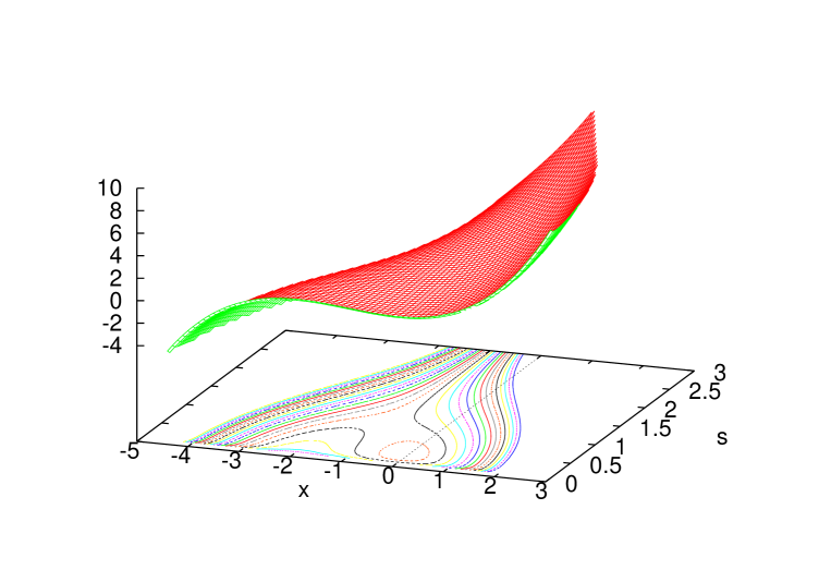
Figure 2: Second-order effective potential for a cubic classical potential. As the contour lines indicate, the classical barrier is lowered in the $s$-direction, making it possible for trajectories to bypass it while conserving energy. The lines also show that there is still a trapped region in this second-order truncation of the quantum potential. Higher-order moments would have to be included in order to describe complete tunneling at all energies.

An application to tunneling immediately follows because we always have $V^{\prime\prime}(q)<0$ around local maxima of the potential, provided it is twice differentiable. The term $\frac{1}{2}V^{\prime\prime}(q)s^{2}$ in the effective potential therefore lowers the potential barrier in the new $s$-direction; see Fig. 2 for an example. Tunneling can then be described by quasiclassical motion in an extended phase space, bypassing the barrier with conserved energy [17, 16]. (See also [18] for an analysis of the same effect directly in terms of moments.)

This application of moment methods shows the importance of keeping $s$ as a degree of freedom that evolves independently of $q$ (while being coupled to it in a specific way). Other effective methods often replace independent degrees of freedom such as $s$ with new $q$-dependent quantum corrections in an effective Hamiltonian, which in general are of higher-derivative form. Such higher-derivative or adiabatic corrections may be derived as a further approximation within our quasiclassical systems. For instance, the general equation

$$\dot{p}_{s}=-\frac{\partial H_{\rm eff}}{\partial s}$$ (37)

provides a differential equation for $p_{s}$ depending on $q$ and $s$ on the right-hand side. If we consider the full effective potential as in Fig. 2, the equation for $\dot{p}_{s}$ is part of the equations of motion that describe a trajectory in the $(q,s)$-plane in which $s$ is kept as a degree of freedom independent of $q$. Several other effective methods, such as those based on path integrals as in [2], do not exhibit new independent degrees of freedom but rather use additional approximations that (explicitly or implicitly) assume adiabatic evolution of quantum variables such as $s$, while there is no such restriction on classical variables such as $q$.

If the evolution of $s$ and its momentum $p_{s}$ is completely ignored, the left-hand side of (37) vanishes, and the equation is turned into an algebraic equation relating $s=s_{0}(q)$ at an extremum of the effective potential, where $\partial H_{\rm eff}/\partial s=0$. If this extremum is a local minimum, the solution is stable, but it does not evolve in $s$ which merely follows the evolution of $q$ in an adiabatic manner. If we insert $s=s_{0}(q)$ as well as $p_{s}=m\dot{s}=m\dot{q}{\rm d}s_{0}(q)/{\rm d}q$ in the effective Hamiltonian, we obtain a position-dependent mass correction of the classical kinetic energy $\frac{1}{2}m\dot{q}^{2}$.

For small oscillations around the minimum, close to the ground state, one may assume that $\dot{p}_{s}$ is small but not exactly zero, and include corresponding deviations $\delta s$ of $s=s_{0}(q)+\delta s$ from its value at the minimum. If one expands the right-hand side of (37) in $\delta s$, it implies a linear equation for $\delta s$ as a function of $\dot{p}_{s}$, which in turn is related to $\ddot{s}$ by Hamilton’s equation for $s$. Inserting $s=s_{0}(q)+\delta s$ with the solutions for $s_{0}(q)$ and $\delta s$ in the effective Hamiltonian implies a higher-derivative correction in an effective Hamiltonian that now depends on second-order derivatives. At higher orders in a systematic adiabatic expansion, derivatives of arbitrary orders appear. In a second-order moment description, all these terms are replaced by the coupled dynamics of a single quantum degree of freedom, $s$.

4 Conclusions

We have presented several examples in which a canonical description of quantum degrees of freedom can lead to new geometrical insights. We have presented examples in which uncertainty relations are replaced by centrifugal barriers in a quasiclassical phase space equipped with non-classical dimensions. Such descriptions may make it easier to study the interplay between uncertainty relations and the dynamics.

The novel formulation presented here, based on the mathematical subject of Poisson geometry, unifies and extends several previous approaches from various fields. Quantum degrees of freedom, up to a given order in $\hbar$, are represented by independent dynamical variables rather than higher-derivative corrections of classical terms obtained from an adiabatic or derivative expansion. Physically, effective Hamiltonians that describe quantum evolution by maintaining the classical number of degrees of freedom require higher derivative terms because quantum dynamics is non-local in time (and also in space in quantum field theory) if one considers only the classical degrees of freedom. Because a wave function is in general spread out, it can have a non-negligible effect on distant points even before one would expect the classical position to reach there. By maintaining fluctuations and higher moments as independent variables, however, the system can still be described by local evolution. The formalism described here therefore provides an efficient and often intuitive description of what would appear as non-adiabatic and non-local quantum effects in other effective descriptions. If extensions to higher orders and multiple degrees of freedom are feasible, there are promising advantages for numerical quantum evolution.

The methods also make it possible to characterize states and to distinguish systematically between classical and quantum states, which may be of advantage in hybrid treatments where some degrees of freedom can be considered classical. Their moments can then be ignored, while other degrees of freedom would couple to their own moments. As seen in our discussion of uncertainty relations, Casimir variables also play a role because they are subject to different bounds in classical and quantum systems. The standard uncertainty relation has a lower bound of $C=0$ in classical physics because a distribution on phase space may be sharply peaked in both $q$ and $p$, but this is no longer possible in quantum physics. In this way, boundaries of quasiclassical phase spaces provide a model independent way to distinguish between classical and quantum systems or their hybrid combinations.

References

- [1] B. O. Koopman, Hamiltonian Systems and Transformations in Hilbert Space, PNAS 17 (1931) 315–318
- [2] F. Cametti, G. Jona-Lasinio, C. Presilla, and F. Toninelli, Comparison between quantum and classical dynamics in the effective action formalism, In Proceedings of the International School of Physics “Enrico Fermi”, Course CXLIII, pages 431–448, Amsterdam, 2000. IOS Press, [quant-ph/9910065]
- [3] S. Coleman and E. Weinberg, Radiative corrections as the origin of spontaneous symmetry breaking, Phys. Rev. D 7 (1973) 1888–1910
- [4] F. Strocchi, Complex coordinates and quantum mechanics, Rev. Mod. Phys. 38 (1966) 36–40
- [5] T. W. B. Kibble, Geometrization of quantum mechanics, Commun. Math. Phys. 65 (1979) 189–201
- [6] A. Heslot, Quantum mechanics as a classical theory, Phys. Rev. D 31 (1985) 1341–1348
- [7] M. Bojowald and A. Skirzewski, Effective Equations of Motion for Quantum Systems, Rev. Math. Phys. 18 (2006) 713–745, [math-ph/0511043]
- [8] R. Jackiw and A. Kerman, Time Dependent Variational Principle And The Effective Action, Phys. Lett. A 71 (1979) 158–162
- [9] F. Arickx, J. Broeckhove, W. Coene, and P. van Leuven, Gaussian Wave-packet Dynamics, Int. J. Quant. Chem.: Quant. Chem. Symp. 20 (1986) 471–481
- [10] R. A. Jalabert and H. M. Pastawski, Environment-independent decoherence rate in classically chaotic systems, Phys. Rev. Lett. 86 (2001) 2490–2493
- [11] O. Prezhdo, Quantized Hamiltonian Dynamics, Theor. Chem. Acc. 116 (2006) 206
- [12] M. Bojowald, D. Brizuela, H. H. Hernandez, M. J. Koop, and H. A. Morales-Técotl, High-order quantum back-reaction and quantum cosmology with a positive cosmological constant, Phys. Rev. D 84 (2011) 043514, [arXiv:1011.3022]
- [13] V. I. Arnold, Mathematical Methods of Classical Mechanics, Springer, 1997
- [14] T. Vachaspati and G. Zahariade, A Classical-Quantum Correspondence and Backreaction, Phys. Rev. D 98 (2018) 065002, [arXiv:1806.05196]
- [15] B. Baytaş, M. Bojowald, and S. Crowe, Faithful realizations of semiclassical truncations, Ann. Phys. 420 (2020) 168247, [arXiv:1810.12127]
- [16] B. Baytaş, M. Bojowald, and S. Crowe, Effective potentials from canonical realizations of semiclassical truncations, Phys. Rev. A 99 (2019) 042114, [arXiv:1811.00505]
- [17] O. Prezhdo and Yu.Ṽ. Pereverzev, Quantized Hamilton Dynamics, J. Chem. Phys. 113 (2000) 6557
- [18] L. Aragon-Muñoz, G. Chacon-Acosta, and H. Hernández-Hernández, Effective quantum tunneling from a semiclassical momentous approach, Int. Mod. J. Phys. B 34 (2020) 2050271, [arXiv:2004.00118]