vZ$withtheperiod$v$equaltothelengthofthevector$v$.\par\begin{dfn}[density functions for periodic sets of points with radii]Letaperiodicset$S=\Lambda+M\subset\mathbb{R}^{n}$haveaunitcell$U$.Foreverypoint$p\in M$,fixaradius$r(p)\geq 0$.Foranyinteger$k\geq 0$,let$U_{k}(t)$betheregionwithinthecell$U$coveredbyexactly$k$closedballs$\bar{B}(p\mathchar 24635\relax\;r(p)+t)$for$t\geq 0$andallpoints$p\in M$andtheirtranslationsby$\Lambda$.The$k$-th\emph{density}function$\psi_{k}[S](t)=\mathrm{Vol}[U_{k}(t)]/\mathrm{Vol}[U]$isthefractionalvolumeofthe$k$-foldintersectionsoftheseballswithin$U$.\hfill$\blacksquare$\end{dfn}\par Thedensity$ψ_k[S](t)$canbeinterpretedastheprobabilitythatarandom(uniformlychosenin$U$)point$q$isatamaximumdistance$t$toexactly$k$ballswithinitialradii$r(p)$andallcenters$p∈S$.\vskip 6.0pt plus 2.0pt minus 2.0pt\par For$k=0$,the$0$-thdensity$ψ_0[S](t)$measuresthefractionalvolumeoftheemptyspacenotcoveredbyanyexpandingballs$¯B(p;r(p)+t)$\vskip 6.0pt plus 2.0pt minus 2.0pt\par Inthesimplestcaseofradii$r(p)=0$,theinfinitesequence$Ψ[S]={ψ_k(t)}_k=0^+∞$wascalledin\cite[cite]{(\@@bibref{AuthorsPhrase1Year}{edels2021}{\@@citephrase{, }}{}, section~{}3)}the\emph{density fingerprint}ofaperiodicpointset$S$.For$k=1$andsmall$t>0$whileallequal-sizedballs$¯B(p;t)$remaindisjoint,the1stdensity$ψ_1[S](t)$increasesproportionallyto$t^n$butlaterreachesamaximumandeventuallydropsbackto$0$whenallpointsof$R^n$arecoveredofbyatleasttwoballs.Seethedensities$ψ_k,k=0,…,8$forthesquareandhexagonallatticesin\cite[cite]{(\@@bibref{AuthorsPhrase1Year}{edels2021}{\@@citephrase{, }}{}, Fig.~{}2)}.\vskip 6.0pt plus 2.0pt minus 2.0pt\par TheoriginaldensitieshelpedfindamissingcrystalintheCambridgeStructuralDatabase,whichwasaccidentallyconfusedwithaslightperturbation(measuredatadifferenttemperature)ofanothercrystal(polymorph)withthesamechemicalcomposition,see\cite[cite]{(\@@bibref{AuthorsPhrase1Year}{edels2021}{\@@citephrase{, }}{}, section~{}7)}.\vskip 6.0pt plus 2.0pt minus 2.0pt\par Thenewweightedcasewithradii$r(p)≥0$inDefinition~{}\ref{dfn:densities}isevenmorepracticallyimportantduetodifferentVanderWaalsradii,whichareindividuallydefinedforallchemicalelements.\vskip 6.0pt plus 2.0pt minus 2.0pt\par Thekeyadvantageofdensityfunctionsoverotherisometryinvariantsofperiodiccrystals(suchassymmetriesorconventionalrepresentationsbasedonageometryofaminimalcell)istheircontinuityunderperturbations,seedetailsinsection~{}\ref{sec:review}reviewingtherelatedpastwork.\vskip 6.0pt plus 2.0pt minus 2.0pt\par Theonlylimitationistheinfinitesizeofdensities$ψ_k(t)$duetotheunboundedparameters:integerindex$k≥0$andcontinuousradius$t≥0$.\vskip 6.0pt plus 2.0pt minus 2.0pt\par Westatethefollowingprobleminfullgeneralitytomotivatefutureworkonthesedensities.\par\begin{pro}[computation of $\psi_k$]Verifyifthedensityfunctions$\psi_{k}[S](t)$fromDefinition~{}\ref{dfn:densities}canbecomputedinapolynomialtime(inthesize$m$ofamotifof$S$)forafixeddimension$n$.\hfill$\blacksquare$\end{pro}\par ThemaincontributionisthefullsolutionofProblem~{}\ref{pro:densities}for$n=1$.Theorems~{}\ref{thm:0-th_density},~{}\ref{thm:1st_density},~{}\ref{thm:k-th_density},~{}\ref{thm:periodicity},andCorollary~{}\ref{cor:computation}efficientlycomputeall$ψ_k[S](t)$dependingoninfinitelymanyvaluesof$k$and$t.

2 Review of related past work

Periodic Geometry was initiated in 2020 by the problem (mosca2020voronoi, section 2.3) to design a computable metric on isometry classes of lattices, which is continuous under perturbations of a lattice basis.

Though a Voronoi domain is combinatorially unstable under perturbations, its geometric shape was used to introduce two continuous metrics (mosca2020voronoi, Theorems 2, 4) requiring approximations due to a minimization over infinitely many rotations.

Similar minimizations over rotations or other continuous parameters are required for the complete invariant isosets anosova2021isometry; anosova2022recognition and density functions, which can be practically computed in low dimensions smith2022practical, whose completeness was proved for generic periodic point sets in $\mathbb{R}^{3}$ (edels2021, Theorem 2). The density fingerprint $\Psi[S]$ turned out to be incomplete (edels2021, section 5) in the example below.

Example 2.1 (periodic sequences $S_{15},Q_{15}\subset\mathbb{R}$).

Widdowson et al. (widdowson2022average, Appendix B) discussed homometric sets that can be distinguished by the invariant AMD (Average Minimum Distances) and not by diffraction patterns. The sequences

$\begin{array}[]{l}S_{15}=\{0,1,3,4,5,7,9,10,12\}+15\mathbb{Z},\\ Q_{15}=\{0,1,3,4,6,8,9,12,14\}+15\mathbb{Z}\end{array}$

have the unit cell $[0,15]$ shown as a circle in Fig. 2.

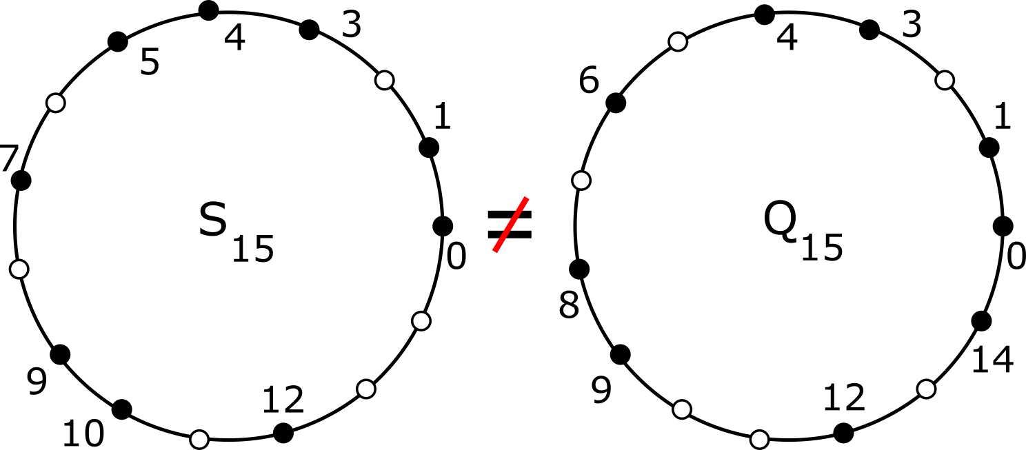
Figure 2: Circular versions of the periodic sets $S_{15},Q_{15}$.

These periodic sequences grunbaum1995use are obtained as Minkowski sums $S_{15}=U+V+15\mathbb{Z}$ and $Q_{15}=U-V+15\mathbb{Z}$ for $U=\{0,4,9\}$, $V=\{0,1,3\}$. $\blacksquare$

For rational-valued periodic sequences, (grunbaum1995use, Theorem 4) proved that $r$-th order invariants (combinations of $r$-factor products) up to $r=6$ are enough to distinguish such sequences up to a shift (a rigid motion of $\mathbb{R}$ without reflections).

The AMD invariant was extended to the Pointwise Distance Distribution (PDD), whose generic completeness (widdowson2022resolving, Theorem 4.4) was proved in any dimension $n\geq 1$. However there are finite sets in $\mathbb{R}^{3}$ (pozdnyakov2020incompleteness, Fig. S4) with the same PDD, which were distinguished by more sophisticated distance-based invariants in (widdowson2021pointwise, appendix C).

The subarea of Lattice Geometry developed continuous parameterizations for the moduli spaces of lattices considered up to isometry in dimension two kurlin2022mathematics; bright2023geographic and three kurlin2022complete; bright2021welcome.

For 1-periodic sequences of points in $\mathbb{R}^{n}$, complete isometry invariants with continuous and computable metrics appeared in kurlin2022exactly, see related results for finite clouds of unlabeled points smith2022families; kurlin2022computable.

3 The 0-th density function $\psi_{0}$

This section proves Theorem 3.2 explicitly describing the 0-th density function $\psi_{0}[S](t)$ for any periodic sequence $S\subset\mathbb{R}$ of disjoint intervals.

For convenience, scale any periodic sequence $S$ to period 1 so that $S$ is given by points $0\leq p_{1}<\cdots<p_{m}<1$ with radii $r_{1},\dots,r_{m}$, respectively. Since the expanding balls in $\mathbb{R}$ are growing intervals, volumes of their intersections linearly change with respect to the variable radius $t$. Hence any density function $\psi_{k}(t)$ is piecewise linear and uniquely determined by corner points $(a_{j},b_{j})$ where the gradient of $\psi_{k}(t)$ changes.

To prepare the proof of Theorem 3.2, we first consider Example 3.1 for the simple sequence $S$.

Example 3.1 ($0$-th density function $\psi_{0}$).

Let the periodic sequence $S=\left\{0,\dfrac{1}{3},\dfrac{1}{2}\right\}+\mathbb{Z}$ have three points $p_{1}=0$, $p_{2}=\dfrac{1}{3}$, $p_{3}=\dfrac{1}{2}$ of radii $r_{1}=\dfrac{1}{12}$, $r_{2}=0$, $r_{3}=\dfrac{1}{12}$, respectively. Fig. 3 shows each point $p_{i}$ and its growing interval L_i(t)=[(p_i-r_i)-t,(p_i+r_i)+t] of the length 2r_i+2t for $i=1,2,3$ in its own color: red, green, blue.

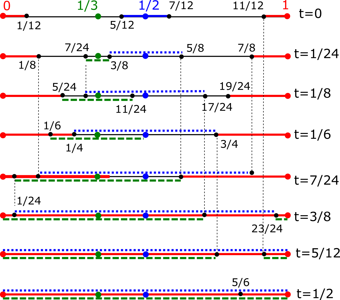
Figure 3: The sequence $S=\left\{0,\dfrac{1}{3},\dfrac{1}{2}\right\}+\mathbb{Z}$ has the points of weights $\dfrac{1}{12},0,\dfrac{1}{12}$, respectively. The growing intervals around the red point $0\equiv 1\pmod{1}$, green point $\dfrac{1}{3}$, blue point $\dfrac{1}{2}$ have the same color for various radii $t$, see Examples 3.1, 4.1, 5.1.

By Definition 1.2 each density function $\psi_{k}[S](t)$ measures a fractional length covered by exactly $k$ intervals within the unit cell $[0,1]$. We periodicaly map the endpoints of each growing interval to the unit cell $[0,1]$. For instance, the interval $[-\dfrac{1}{12}-t,\dfrac{1}{12}+t]$ of the point $p_{1}=0\equiv 1\pmod{1}$ maps to the red intervals $[0,\dfrac{1}{12}+t]\cup[\dfrac{11}{12}-t,1]$ shown by solid red lines in Fig. 3. The same image shows the green interval $[\dfrac{1}{3}-t,\dfrac{1}{3}+t]$ by dashed lines and the blue interval $[\dfrac{5}{12}-t,\dfrac{7}{12}+t]$ by dotted lines.

At the moment $t=0$, since the starting intervals are disjoint, they cover the length $l=2(\dfrac{1}{12}+0+\dfrac{1}{12})=\dfrac{1}{3}$. The non-covered part of $[0,1]$ has length $1-\dfrac{1}{3}=\dfrac{2}{3}$. So the graph of $\psi_{0}(t)$ at $t=0$ starts from the point $(0,\dfrac{2}{3})$, see Fig. 4.

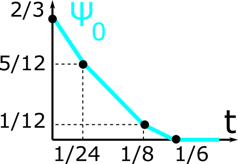
Figure 4: The 0-th density function $\psi_{0}(t)$ for the 1-period sequence $S$ whose points $0,\dfrac{1}{3},\dfrac{1}{2}$ have radii $\dfrac{1}{12},0,\dfrac{1}{12}$, respectively, see Example 3.1.

At the first critical moment $t=\dfrac{1}{24}$ when the green and blue intervals collide at $p=\dfrac{3}{8}$, only the intervals $[\dfrac{1}{8},\dfrac{7}{24}]\cup[\dfrac{5}{8},\dfrac{7}{8}]$ of total length $\dfrac{5}{12}$ remain uncovered. Hence $\psi_{0}(t)$ linearly drops to the point $(\dfrac{1}{12},\dfrac{5}{12})$. At the next critical moment $t=\dfrac{1}{8}$ when the red and green intervals collide at $p=\dfrac{5}{24}$, only the interval $[\dfrac{17}{24},\dfrac{19}{24}]$ of length $\dfrac{1}{12}$ remain uncovered, so $\psi_{0}(t)$ continues to $(\dfrac{1}{8},\dfrac{1}{12})$.

The graph of $\psi_{0}(t)$ finally returns to the $t$-axis at the point $(\dfrac{1}{6},0)$ and remains there for $t\geq\dfrac{1}{6}$.

The piecewise linear behavior of $\psi_{0}(t)$ can be described by specifying the corner points in Fig. 4: $\left(0,\dfrac{2}{3}\right)$, $\left(\dfrac{1}{24},\dfrac{5}{12}\right)$, $\left(\dfrac{1}{8},\dfrac{1}{12}\right)$, $\left(\dfrac{1}{6},0\right)$. $\blacksquare$

Theorem 3.2 extends Example 3.1 to any periodic sequence $S$ and implies that the 0-th density function $\psi_{0}(t)$ is uniquely determined by the ordered gap lengths between successive intervals.

Theorem 3.2 (description of $\psi_{0}$).

Let a periodic sequence $S=\{p_{1},\dots,p_{m}\}+\mathbb{Z}$ consist of disjoint intervals with centers $0\leq p_{1}<\dots<p_{m}<1$ and radii $r_{1},\dots,r_{m}\geq 0$. Consider the total length $l=2\sum\limits_{i=1}^{m}r_{i}$ and gaps between successive intervals $g_{i}=(p_{i}-r_{i})-(p_{i-1}+r_{i-1})$, where $i=1,\dots,m$ and $p_{0}=p_{m}-1$, $r_{0}=r_{m}$. Put the gaps in increasing order: $g_{[1]}\leq g_{[2]}\leq\dots\leq g_{[m]}$.

Then the 0-th density $\psi_{0}[S](t)$ is piecewise linear with the following (unordered) corner points: $(0,1-l)$ and $\left(\dfrac{g_{[i]}}{2},\;1-l-\sum\limits_{j=1}^{i-1}g_{[j]}-(m-i+1)g_{[i]}\right)$ for $i=1,\dots,m$, so the last corner is $\left(\dfrac{g_{[m]}}{2},0\right)$.

If any corners are repeated, e.g. when $g_{[i-1]}=g_{[i]}$, these corners are collapsed into one corner. $\blacksquare$

Proof: By Definition 1.2 the 0-th density function $\psi_{0}(t)$ measures the total length of subintervals in the unit cell $[0,1]$ that are not covered by any of the growing intervals $L_{i}(t)=[p_{i}-r_{i}-t,p_{i}+r_{i}+t]$, $i=1,\dots,m$. For $t=0$, since all initial intervals $L_{i}(0)$ are disjoint, they cover the total length $2\sum\limits_{i=1}^{m}r_{i}=l$.

Then the graph of $\psi_{0}(t)$ at $t=0$ starts from the point $(0,1-l)$. So $\psi_{0}(t)$ linearly decreases from the initial value $\psi_{0}(0)=1-l$ except for $m$ critical values of $t$ where one of the gap intervals $[p_{i}+r_{i}+t,p_{i+1}-r_{i+1}-t]$ between successive growing intervals $L_{i}(t)$ and $L_{i+1}(t)$ shrinks to a point. These critical radii $t$ are ordered according to the gaps $g_{[1]}\leq g_{[2]}\leq\dots\leq g_{[m]}$.

The first critical radius is $t=\dfrac{1}{2}g_{[1]}$, when a shortest gap interval of the length $g_{[1]}$ is covered by the growing successive intervals. At this moment $t=\dfrac{1}{2}g_{[1]}$, all $m$ growing intervals $L_{i}(t)$ have the total length $l+mg_{[1]}$. Then the 0-th density $\psi_{0}(t)$ has the first corner points $(0,1-l)$ and $\left(\dfrac{g_{[1]}}{2},1-l-mg_{[1]}\right)$.

The second critical radius is $t=\dfrac{g_{[2]}}{2}$, when all intervals $L_{i}(t)$ have the total length $l+g_{[1]}+(m-1)g_{[2]}$, i.e. the next corner point is $\left(\dfrac{g_{[2]}}{2},1-l-g_{[1]}-(m-1)g_{[2]}\right)$. If $g_{[1]}=g_{[2]}$, then both corner points coincide, so $\psi_{0}(t)$ will continue from the joint corner point.

The above pattern generalizes to the $i$-th critical radius $t=\dfrac{1}{2}g_{[i]}$, when all covered intervals have the total length $\sum\limits_{j=1}^{i-1}g_{[j]}$ (for the fully covered intervals) plus $(m-i+1)g_{[i]}$ (for the still growing intervals).

For the final critical radius $t=\dfrac{g_{[m]}}{2}$, the whole unit cell $[0,1]$ is covered by the grown intervals because $\sum\limits_{j=1}^{m}g_{[j]}=1-l$. The final corner is $(\dfrac{g_{[m]}}{2},0)$.

Example 3.3 applies Theorem 3.2 to get $\psi_{0}$ found for the periodic sequence $S$ in Example 3.1.

Example 3.3 (using Theorem 3.2).

The sequence $S=\left\{0,\dfrac{1}{3},\dfrac{1}{2}\right\}+\mathbb{Z}$ in Example 3.1 with points $p_{1}=0$, $p_{2}=\dfrac{1}{3}$, $p_{3}=\dfrac{1}{2}$ of radii $r_{1}=\dfrac{1}{12}$, $r_{2}=0$, $r_{3}=\dfrac{1}{12}$, respectively, has $l=2(r_{1}+r_{2}+r_{3})=\dfrac{1}{3}$ and the initial gaps between successive intervals $g_{1}=p_{1}-r_{1}-p_{3}-r_{3}=(1-\dfrac{1}{12})-(\dfrac{1}{2}+\dfrac{1}{12})=\dfrac{1}{3}$,

$g_{2}=p_{2}-r_{2}-p_{1}-r_{1}=(\dfrac{1}{3}-0)-(0+\dfrac{1}{12})=\dfrac{1}{4}$,

$g_{3}=p_{3}-r_{3}-p_{2}-r_{2}=(\dfrac{1}{2}-\dfrac{1}{12})-(\dfrac{1}{3}+0)=\dfrac{1}{12}$. Order the gaps: $g_{[1]}=\dfrac{1}{12}<g_{[2]}=\dfrac{1}{4}<g_{[3]}=\dfrac{1}{3}$. $1-l=1-\dfrac{1}{3}=\dfrac{2}{3}$,

$1-l-3g_{[1]}=\dfrac{2}{3}-\dfrac{3}{12}=\dfrac{5}{12}$,

$1-l-g_{[1]}-2g_{[2]}=\dfrac{2}{3}-\dfrac{1}{12}-\dfrac{2}{4}=\dfrac{1}{12}$,

$1-l-g_{[1]}-g_{[2]}-g_{[3]}=\dfrac{2}{3}-\dfrac{1}{12}-\dfrac{1}{4}-\dfrac{1}{3}=0$.
By Theorem 3.2 $\psi_{0}(t)$ has the corner points $(0,1-l)=\left(0,\dfrac{2}{3}\right)$,

$\left(\dfrac{1}{2}g_{[1]},1-l-3g_{[1]}\right)=\left(\dfrac{1}{24},\dfrac{5}{12}\right)$,

$\left(\dfrac{1}{2}g_{[2]},1-l-g_{[1]}-2g_{[2]}\right)=\left(\dfrac{1}{8},\dfrac{1}{12}\right)$,

$\left(\dfrac{1}{2}g_{[3]},1-l-g_{[1]}-g_{[2]}-g_{[3]}\right)=\left(\dfrac{1}{6},0\right)$. See the graph of the 0-th density $\psi_{0}(t)$ in Fig. 4. $\blacksquare$

By Theorem 3.2 any 0-th density function $\psi_{0}(t)$ is uniquely determined by the (unordered) set of gap lengths between successive intervals. Hence we can re-order these intervals without changing $\psi_{0}(t)$. For instance, the periodic sequence $Q=\{0,\dfrac{1}{2},\dfrac{2}{3}\}+\mathbb{Z}$ with points $0,\dfrac{1}{2},\dfrac{2}{3}$ of weights $\dfrac{1}{12},\dfrac{1}{12},0$ has the same set ordered gaps $g_{[1]}=\dfrac{1}{12}$, $d_{[2]}=\dfrac{1}{3}$, $d_{[3]}=\dfrac{1}{2}$ as the periodic sequence $S=\left\{0,\dfrac{1}{3},\dfrac{1}{2}\right\}+\mathbb{Z}$ in Example 3.1.

The above sequences $S,Q$ are related by the mirror reflection $t\mapsto 1-t$. One can easily construct many non-isometric sequences with $\psi_{0}[S](t)=\psi_{0}[Q](t)$. For any $1\leq i\leq m-3$, the sequences $S_{m,i}=\{0,2,3,\dots,i+2,i+4,i+5,\dots,m+2\}+(m+2)\mathbb{Z}$ have the same interval lengths $d_{[1]}=\dots=d_{[m-2]}=1$, $d_{[m-1]}=d_{[m]}=2$ but are not related by isometry (translations and reflections in $\mathbb{R}$) because the intervals of length 2 are separated by $i-1$ intervals of length 1 in $S_{m,i}$.

4 The 1st density function $\psi_{1}$

This section proves Theorem 4.2 explicitly describing the 1st density $\psi_{1}[S](t)$ for any periodic sequence $S$ of disjoint intervals. To prepare the proof of Theorem 4.2, Example 4.1 finds $\psi_{1}[S]$ for the sequence $S$ from Example 3.1.

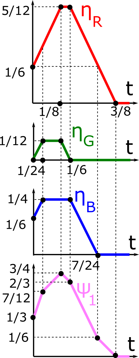
Figure 5: The trapezoid functions $\eta_{R},\eta_{G},\eta_{B}$ and the 1st density function $\psi_{1}(t)$ for the 1-period sequence $S$ whose points $0,\dfrac{1}{3},\dfrac{1}{2}$ have radii $\dfrac{1}{12},0,\dfrac{1}{12}$, see Example 4.1.

Example 4.1 ($\psi_{1}$ for $S=\left\{0,\dfrac{1}{3},\dfrac{1}{2}\right\}+\mathbb{Z}$).

The 1st density function $\psi_{1}(t)$ can be obtained as a sum of the three trapezoid functions $\eta_{R}$, $\eta_{G}$, $\eta_{B}$, each measuring the length of a region covered by a single interval of one color, see Fig. 3.

At the initial moment $t=0$, the red intervals $[0,\dfrac{1}{12}]\cup[\dfrac{11}{12},1]$ have the total length $\eta_{R}(0)=\dfrac{1}{6}$. These red intervals $[0,\dfrac{1}{12}+t]\cup[\dfrac{11}{12}-t,1]$ for $t\in[0,\dfrac{1}{8}]$ grow until they touch the green interval $[\dfrac{7}{24},\dfrac{3}{8}]$ and have the total length $\eta_{R}(\dfrac{1}{8})=\dfrac{1}{6}+\dfrac{2}{8}=\dfrac{5}{12}$ in the second picture of Fig. 3. So the graph of the red length $\eta_{R}(t)$ linearly grows with gradient 2 from the point $(0,\dfrac{1}{6})$ to the corner point $(\dfrac{1}{8},\dfrac{5}{12})$.

For $t\in[\dfrac{1}{8},\dfrac{1}{6}]$, the left red interval is shrinking at the same rate (due to the overlapping green interval) as the right red interval continues to grow until $t=\dfrac{1}{6}$, when it touches the blue interval $[\dfrac{1}{4},\dfrac{3}{4}]$. Hence the graph of $\eta_{R}(t)$ remains constant for $t\in[\dfrac{1}{8},\dfrac{1}{6}]$ up to the corner point $(\dfrac{1}{6},\dfrac{5}{12})$.

After that, the graph of $\eta_{R}(t)$ linearly decreases (with gradient $-2$) until all red intervals are fully covered by the green and blue intervals at moment $t=\dfrac{3}{8}$, see the 6th picture in Fig. 3.

Hence the trapezoid function $\eta_{R}$ has the piecewise linear graph through the corner points $(0,\dfrac{1}{6})$, $(\dfrac{1}{8},\dfrac{5}{12})$, $(\dfrac{1}{6},\dfrac{5}{12})$, $(\dfrac{3}{8},0)$. After that, $\eta_{R}(t)=0$ remains constant for $t\geq\dfrac{3}{8}$. Fig. 5 shows the graphs of $\eta_{R},\eta_{G},\eta_{B}$ and $\psi_{1}=\eta_{R}+\eta_{G}+\eta_{B}$. $\blacksquare$

Theorem 4.2 extends Example 4.1 and proves that any $\psi_{1}(t)$ is a sum of trapezoid functions whose corners are explicitly described. We consider any index $i=1,\dots,m$ (of a point $p_{i}$ or a gap $g_{i}$) modulo $m$ so that $m+1\equiv 1\pmod{m}$.

Theorem 4.2 (description of $\psi_{1}$).

Let a periodic sequence $S=\{p_{1},\dots,p_{m}\}+\mathbb{Z}$ consist of disjoint intervals with centers $0\leq p_{1}<\dots<p_{m}<1$ and radii $r_{1},\dots,r_{m}\geq 0$, respectively.

Consider the gaps $g_{i}=(p_{i}-r_{i})-(p_{i-1}+r_{i-1})$, where $i=1,\dots,m$ and $p_{0}=p_{m}-1$, $r_{0}=r_{m}$.

Then the 1st density $\psi_{1}(t)$ is the sum of $m$ trapezoid functions $\eta_{i}$, $i=1,\dots,m$, with the corners $(0,2r_{i})$, $\left(\dfrac{g_{i}}{2},g+2r_{i}\right)$, $\left(\dfrac{g_{i+1}}{2},g+2r_{i}\right)$, $\left(\dfrac{g_{i}+g_{i+1}}{2}+r_{i},0\right),$ where $g=\min\{g_{i},g_{i+1}\}$.

Hence $\psi_{1}(t)$ is determined by the unordered set of unordered pairs $(g_{i},g_{i+1})$, $i=1,\dots,m$. $\blacksquare$

Proof: The 1st density $\psi_{1}(t)$ equals the total length of subregions covered by exactly one of the intervals $L_{i}(t)=[p_{i}-r_{i}-t,p_{i}+r_{i}+t]$, $i=1,\dots,m$, where all intervals are taken modulo 1 within $[0,1]$.

Hence $\psi_{1}(t)$ is the sum of the functions $\eta_{1i}$, each measuring the length of the subinterval of $L_{i}(t)$ not covered by other intervals $L_{j}(t)$, $j\in\{1,\dots,m\}-\{i\}$.

Since the initial intervals $L_{i}(0)$ are disjoint, each function $\eta_{1i}(t)$ starts from the value $\eta_{1i}(0)=2r_{i}$ and linearly grows (with gradient 2) up to $\eta_{i}(\dfrac{1}{2}g)=2r_{i}+g$, where $g=\min\{g_{i},g_{i+1}\}$, when the growing interval $L_{i}(t)$ of the length $2r_{i}+2t=2r_{i}+g$ touches its closest neighboring interval $L_{i\pm 1}(t)$ with a shortest gap $g$.

If (say) $g_{i}<g_{i+1}$, then the subinterval covered only by $L_{i}(t)$ is shrinking on the left and is growing at the same rate on the right until $L_{i}(t)$ touches the growing interval $L_{i+1}(t)$ on the right. During this growth, when $t$ is between $\dfrac{1}{2}g_{i}$ and $\dfrac{1}{2}g_{i+1}$, the trapezoid function $\eta_{i}(t)=g$ remains constant.

If $g_{i}=g_{i+1}$, this horizontal line collapses to one point in the graph of $\eta_{i}(t)$. For $t\geq\max\{g_{i},g_{i+1}\}$, the subinterval covered only by $L_{i}(t)$ is shrinking on both sides until the neighboring intervals $L_{i\pm 1}(t)$ meet at a mid-point between their initial closest endpoints $p_{i-1}+r_{i-1}$ and $p_{i+1}-r_{i+1}$. This meeting time is $t=\dfrac{1}{2}(p_{i+1}-r_{i+1}-p_{i-1}-r_{i-1})=\dfrac{1}{2}(g_{i}+2r_{i}+g_{i+1})$, which is also illustrated by Fig. 6. So the trapezoid function $\eta_{i}$ has the corners $(0,2r_{i})$, $\left(\dfrac{g_{i}}{2},2r_{i}+g\right)$, $\left(\dfrac{g_{i+1}}{2},2r_{i}+g\right)$, $\left(\dfrac{g_{i}+g_{i+1}}{2}+r_{i},0\right)$ as expected.

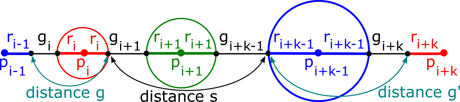
Figure 6: The distances $g,s,g^{\prime}$ between line intervals used in the proofs of Theorems 4.2 and 5.2, shown here for $k=3$.

Example 4.3 applies Theorem 4.2 to get $\psi_{1}$ found for the periodic sequence $S$ in Example 4.1.

Example 4.3 (using Theorem 4.2 for $\psi_{1}$).

The sequence $S=\left\{0,\dfrac{1}{3},\dfrac{1}{2}\right\}+\mathbb{Z}$ in Example 4.1 with points $p_{1}=0$, $p_{2}=\dfrac{1}{3}$, $p_{3}=\dfrac{1}{2}$ of radii $r_{1}=\dfrac{1}{12}$, $r_{2}=0$, $r_{3}=\dfrac{1}{12}$, respectively, has the initial gaps between successive intervals $g_{1}=\dfrac{1}{3}$, $g_{2}=\dfrac{1}{4}$, $g_{3}=\dfrac{1}{12}$, see all the computations in Example 3.3.

Case (R). In Theorem 4.2 for the trapezoid function $\eta_{R}=\eta_{1}$ measuring the fractional length covered only by the red interval, we set $k=1$ and $i=1$. Then $r_{i}=\dfrac{1}{12}$, $g_{i}=\dfrac{1}{3}$ and $g_{i+1}=\dfrac{1}{4}$, so gi+gi+12+r_i=12(13+14)+112=38, $g=\min\{g_{i},g_{i+1}\}=\dfrac{1}{4}$, $g+2r_{i}=\dfrac{1}{4}+\dfrac{2}{12}=\dfrac{5}{12}$.

Then $\eta_{R}=\eta_{1}$ has the following corner points: (0,2r_i)=(0,16),  (gi2,g+2r_i)=(16,512),(gi+12,g+2r_i)=(18,512),(gi+gi+12+r_i,0)=(38,0), where the two middle corners are accidentally swapped due to $g_{i}>g_{i+1}$ but they define the same trapezoid function as in the first picture of Fig. 5.

Case (G). In Theorem 4.2 for the trapezoid function $\eta_{G}=\eta_{2}$ measuring the fractional length covered only by the green interval, we set $k=1$ and $i=2$. Then $r_{i}=0$, $g_{i}=\dfrac{1}{4}$ and $g_{i+1}=\dfrac{1}{12}$, so gi+gi+12+r_i=12(14+112)+0=16, $g=\min\{g_{i},g_{i+1}\}=\dfrac{1}{12}$, $g+2r_{i}=\dfrac{1}{12}+0=\dfrac{1}{12}$.

Then $\eta_{G}=\eta_{2}$ has the following corner points exactly as shown in the second picture of Fig. 5: (0,2r_i)=(0,0),  (gi2,g+2r_i)=(18,112),(gi+12,g+2r_i)=(124,512),(gi+gi+12+r_i,0)=(16,0).

Case (B). In Theorem 4.2 for the trapezoid function $\eta_{B}=\eta_{3}$ measuring the fractional length covered only by the blue interval, we set $k=1$ and $i=3$. Then $r_{i}=\dfrac{1}{12}$, $g_{i}=\dfrac{1}{12}$ and $g_{i+1}=\dfrac{1}{3}$, so gi+gi+12+r_i=12(112+13)+112=724, $g=\min\{g_{i},g_{i+1}\}=\dfrac{1}{12}$, $g+2r_{i}=\dfrac{1}{12}+\dfrac{2}{12}=\dfrac{1}{4}$.

Then $\eta_{B}=\eta_{3}$ has the following corner points: (0,2r_i)=(0,16),  (gi2,g+2r_i)=(124,14),(gi+12,g+2r_i)=(16,14),(gi+gi+12+r_i,0)=(724,0) exactly as shown in the third picture of Fig. 5. $\blacksquare$

5 Higher density functions $\psi_{k}$

This section proves Theorem 5.2 describing the $k$-th density function $\psi_{k}[S](t)$ for any $k\geq 2$ and a periodic sequence $S$ of disjoint intervals.

To prepare the proof of Theorem 5.2, Example 5.1 computes $\psi_{2}[S]$ for $S$ from Example 3.1.

Example 5.1 ($\psi_{2}$ for $S=\left\{0,\dfrac{1}{3},\dfrac{1}{2}\right\}+\mathbb{Z}$).

The density $\psi_{2}(t)$ can be found as the sum of the trapezoid functions $\eta_{GB},\eta_{BR},\eta_{RG}$, each measuring the length of a double intersection, see Fig. 3.

For the green interval $[\dfrac{1}{3}-t,\dfrac{1}{3}+t]$ and the blue interval $[\dfrac{5}{12}-t,\dfrac{7}{12}+t]$, the graph of the function $\eta_{GB}(t)$ is piecewise linear and starts at the point $(\dfrac{1}{24},0)$ because these intervals touch at $t=\dfrac{1}{24}$.

The green-blue intersection $[\dfrac{5}{12}-t,\dfrac{1}{3}+t]$ grows until $t=\dfrac{1}{6}$, when the resulting interval $[\dfrac{1}{4},\dfrac{1}{2}]$ touches the red interval on the left. At the same time, the graph of $\eta_{GB}(t)$ is linearly growing (with gradient 2) to the corner $(\dfrac{1}{6},\dfrac{1}{4})$, see Fig, 7.

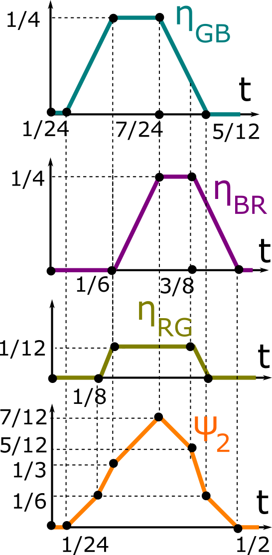
Figure 7: The trapezoid functions $\eta_{GB},\eta_{BR},\eta_{RG}$ and the 2nd density function $\psi_{2}(t)$ for the 1-period sequence $S$ whose points $0,\dfrac{1}{3},\dfrac{1}{2}$ have radii $\dfrac{1}{12},0,\dfrac{1}{12}$, see Example 5.1.

For $t\in[\dfrac{1}{6},\dfrac{7}{24}]$, the green-blue intersection interval becomes shorter on the left, but grows at the same rate on the right until $t=\dfrac{7}{24}$ when $[\dfrac{1}{8},\dfrac{5}{8}]$ touches the red interval $[\dfrac{5}{8},1]$ on the right, see the 5th picture in Fig. 3. So the graph of $\eta_{GB}(t)$ remains constant up to the point $(\dfrac{7}{24},\dfrac{1}{4})$.

For $t\in[\dfrac{7}{24},\dfrac{5}{12}]$ the green-blue intersection interval is shortening from both sides. So the graph of $\eta_{GB}(t)$ linearly decreases (with gradient $-2$) and returns to the $t$-axis at the corner $(\dfrac{5}{12},0)$, then remains constant $\eta_{GB}(t)=0$ for $t\geq\dfrac{5}{12}$.

Fig. 7 shows all trapezoid functions for double intersections and $\psi_{2}=\eta_{GB}+\eta_{BR}+\eta_{RG}$. $\blacksquare$

Theorem 5.2 (description of $\psi_{k}$ for $k\geq 2$).

Let a periodic sequence $S=\{p_{1},\dots,p_{m}\}+\mathbb{Z}$ consist of disjoint intervals with centers $0\leq p_{1}<\dots<p_{m}<1$ and radii $r_{1},\dots,r_{m}\geq 0$, respectively. Consider the gaps $g_{i}=(p_{i}-r_{i})-(p_{i-1}+r_{i-1})$ between the successive intervals of $S$, where $i=1,\dots,m$ and $p_{0}=p_{m}-1$, $r_{0}=r_{m}$.

For $k\geq 2$, the density function $\psi_{k}(t)$ equals the sum of $m$ trapezoid functions $\eta_{k,i}(t)$, $i=1,\dots,m$, each having the following corner points: (s2,0), (g+s2,g), (s+g’2,g), (g+s+g’2,0), where $g,g^{\prime}$ are the minimum and maximum values in the pair $\{g_{i}+2r_{i},g_{i+k}+2r_{i+k-1}\}$, and $s=\sum\limits_{j=i+1}^{i+k-1}g_{j}+2\sum\limits_{j=i+1}^{i+k-2}r_{j}$, so $s=g_{i+1}$ for $k=2$.

Hence $\psi_{k}(t)$ is determined by the unordered set of the ordered tuples $(g,s,g^{\prime})$, $i=1,\dots,m$. $\blacksquare$

Proof: The $k$-th density function $\psi_{k}(t)$ measures the total fractional length of $k$-fold intersections among $m$ intervals $L_{i}(t)=[p_{i}-r_{i}-t,p_{i}+r_{i}+t]$, $i=1,\dots,m$. Now we visualize all such intervals $L_{i}(t)$ in the line $\mathbb{R}$ without mapping them modulo 1 to the unit cell $[0,1]$.

Since all radii $r_{i}\geq 0$, only $k$ successive intervals can contribute to $k$-fold intersections. So a $k$-fold intersection of growing intervals emerges only when two intervals $L_{i}(t)$ and $L_{i+k-1}(t)$ overlap because their intersection should be also covered by all the intermediate intervals $L_{i}(t),L_{i+1}(t),\dots,L_{i+k-1}(t)$.

Then the density $\psi_{k}(t)$ equals the sum of the $m$ trapezoid functions $\eta_{k,i}$, $i=1,\dots,m$, each equal to the length of the $k$-fold intersection $\cap_{j=i}^{i+k-1}L_{j}(t)$ not covered by other intervals. Then $\eta_{k,i}(t)$ remains 0 until the first critical moment $t$ when $2t$ equals the distance between the points $p_{i}+r_{i}$ and $p_{i+k-1}-r_{i+k-1}$ in $\mathbb{R}$, see Fig. 6, so $2t=\sum\limits_{j=i+1}^{i+k-1}g_{j}+2\sum\limits_{j=i+1}^{i+k-2}r_{j}=s$. Hence $t=\dfrac{s}{2}$ and $(\dfrac{s}{2},0)$ is the first corner point of $\eta_{k,i}(t)$.

At $t=\dfrac{s}{2}$, the interval of the $k$-fold intersection $\cap_{j=i}^{i+k-1}L_{j}(t)$ starts expanding on both sides. Hence $\eta_{k,i}(t)$ starts increasing (with gradient 2) until the $k$-fold intersection touches one of the neighboring intervals $L_{i-1}(t)$ or $L_{i+k}(t)$ on the left or on the right.

The left interval $L_{i-1}(t)$ touches the $k$-fold intersection $\cap_{j=i}^{i+k-1}L_{j}(t)$ when $2t$ equals the distance from $p_{i-1}+r_{i-1}$ (the right endpoint of $L_{i-1}$) to $p_{i+k-1}-r_{i+k-1}$ (the left endpoint of $L_{i+k-1}$), see Fig. 6, so 2t=∑_j=i^i+k-1g_j+2∑_j=i^i+k-2 r_j=g_i+2r_i+s.

The right interval $L_{i+k-1}(t^{\prime})$ touches the $k$-fold intersection $\cap_{j=i}^{i+k-1}L_{j}(t^{\prime})$ when $2t^{\prime}$ equals the distance from $p_{i}+r_{i}$ (the right endpoint of $L_{i}$) to $p_{i+k}-r_{i+k}$ (the left endpoint of $L_{i+k}$), see Fig. 6, so 2t’=∑_j=i+1^i+kg