Toward Theoretical Guidance for Two Common Questions in Practical Cross-Validation based Hyperparameter Selection

Abstract

We show, to our knowledge, the first theoretical treatments of two common questions in cross-validation based hyperparameter selection:  After selecting the best hyperparameter using a held-out set, we train the final model using all of the training data – since this may or may not improve future generalization error, should one do this?  During optimization such as via SGD (stochastic gradient descent), we must set the optimization tolerance $\rho$ – since it trades off predictive accuracy with computation cost, how should one set it? Toward these problems, we introduce the hold-in risk (the error due to not using the whole training data), and the model class mis-specification risk (the error due to having chosen the wrong model class) in a theoretical view which is simple, general, and suggests heuristics that can be used when faced with a dataset instance. In proof-of-concept studies in synthetic data where theoretical quantities can be controlled, we show that these heuristics can, respectively,  always perform at least as well as always performing retraining or never performing retraining,  either improve performance or reduce computational overhead by $2\times$ with no loss in predictive performance.

1 Introduction

The learning process has various sources of errors. The first step in (supervised) learning is the acquisition of (training) data. Given data, we choose a model or function class $\mathcal{F}$ which corresponds to not just a method (such as Support Vector Machines, Generalized Linear Models, Neural Networks, Decision trees) but their specific configuration governed by their respective hyperparameters (such as regularization forms and penalties, trees depth) – these hyperparameters refer to anything that would affect the predictive performance of the model learned from the training data. Given our choice of the function class, the learning process searches for the function that (approximately) minimizes the empirical risk (or some surrogate of it which better represents the true risk or is easier to optimize). We currently have an understanding of the factors (Vapnik, 2006; Devroye et al., 2013; Bottou and Bousquet, 2008) affecting the excess risk of this chosen function – (i) the choice of the function class and its capacity to model the data generating process, (ii) the use of an empirical risk estimate instead of the true risk, and (iii) the approximation in the empirical risk minimization (ERM).

However, in practice, the learning process is not limited to these steps. A significant part of the whole exercise is the choice of the function class $\mathcal{F}$ (method and its specifications). Usually, we consider a (possibly large) set of function classes and select one of them based on the data-driven process of model selection or hyperparameter selection. This search can be done via grid search (searching over a discretized grid of hyperparameter values) or random search (Bergstra and Bengio, 2012). However, AutoML (automated machine learning) has spurred a lot of research in the area of hyperparameter optimization or HPO (Hutter et al., 2011; Shahriari et al., 2016; Snoek et al., 2012; Bergstra et al., 2011, 2013). The automation allows us to look at even larger sets of function classes for improved performance while being significantly more efficient than grid search and more accurate than random search. The problem of HPO has been extended from machine learning (ML) model configurations to the design of complete ML pipelines known as the Combined Algorithm Selection and HPO (or CASH) problem, with various schemes that handle (i) pipelines with fixed architecture (Hutter et al., 2011; Bergstra et al., 2011; Rakotoarison et al., 2019; Liu et al., 2020; Kishimoto et al., 2022), (ii) searching over the pipeline architectures (Katz et al., 2020; Marinescu et al., 2021), (iii) deployment and fairness constraints (Liu et al., 2020; Ram et al., 2020), and (iv) operating in the decentralized setting (Zhou et al., 2021, 2022), leading to multiple open-source tools (Thornton et al., 2012; Kotthoff et al., 2017; Feurer et al., 2015, 2020; Komer et al., 2014; Bergstra et al., 2015; Baudart et al., 2020, 2021; Hirzel et al., 2022).

There has also been a significant amount of theoretical work on development of data-dependent penalties for penalty-based model selection, resulting in guarantees in the form of “oracle inequalities” – the expected excess risk of the selected model can be shown to be within a multiplicative and additive factor of the best possible excess risk if an oracle provided us with the best hyperparameter. This has been widely studied in (binary) classification (Boucheron et al., 2005), (bounded) regression and density estimation (Massart, 2007; Arlot et al., 2010). However, in practice, penalty-based model selection is not used for data-driven hyperparameter selection, and we resort to some form of cross-validation(CV). These universally applicable CV techniques have been shown to be theoretically competitive to the penalty-based schemes at the cost of having less data for the learning since some amount of data is “held-out” from the training data for validation purposes (Boucheron et al., 2005; Arlot et al., 2010). We focus on these universal CV based HPO.

Our contributions.

While CV based model selection has been studied theoretically, there are various questions in practical HPO, which have not been explored in literature. A common practice is the learning of the final model on the selected hyperparameter with all available data, reintroducing the held-out data in the training. This is standard practice in many commercial ML tools since user data is too precious to not include in the training of the deployed model. In this paper, we provide answers for the following questions:

A common practice is to approximate the ERM with a large tolerance during the HPO and perform a more accurate ERM during the final model training on the selected HP to reduce the overall computational costs. We study the following related questions:

Note that these answers can be utilized both by humans and by automated data science systems.

Practical motivations.

In applications with large amount of data, the importance of question Q1a (and consequently Q1b) might appear minimal (the computational aspect of questions Q2a and Q2b make them critical with large data). However, we believe that even in such cases, the important signal can still be quite small, and the relevant information in the held-out set can have large impact (positive or negative) on the final deployed model. For example, in various data science applications in finance, the class/target of interest is usually very small. In the Home Credit Default Risk Kaggle Classification Challenge, the training data has only around $8.5\%$ of some $3\times 10^{5}$ training examples from the positive class, and in the AllState Claim Prediction Kaggle Regression Challenge, the training set has less than $1\%$ of some $13\times 10^{6}$ examples with nonzero regression targets; rest are zero. Furthermore, there are situations where the population has groups and the underrepresented minority groups are significantly smaller than the majority group(s). In this case, the presence or absence of the held-out data can have significant (again positive or negative) impact on the fairness and accuracy of the deployed model since many of the fairness metrics quantify the parity in the group specific predictive performance. Finally, “small” differences in predictive performance can have significant impact depending on problems and applications – in data science leaderboards such as Kaggle, minor changes in final performance can lead to significant reordering of the leaderboard (although, relevance of such competitions and results to practical problems remain an open question). Such scenarios motivate us to study the question of whether the practice of retraining after reintroducing the data held-out during HPO is helpful (Q1a).

Empirical motivation.

As evidence of the lack of clarity on this whether question, we consider HPO for LightGBM (Ke et al., 2017) on 40 OpenML (Vanschoren et al., 2013) data sets (we detail the evaluation setup in §2.2). Of the 400 different HPO problems we solve, retraining has (i) no significant effect (positive or negative) in 51/400 (12.75%) cases, (ii) has a positive effect (improving test error) in 260/400 (65%) cases, and (iii) has a negative effect in 89/400 (22.25%) cases. This highlights that there is no single universal correct answer to this question. Hence, we study this whether question rigorously and provide a theoretically motivated data-driven heuristic as one answer.

Outline.

We present our precise problem setting, and existing & novel excess risk decompositions with empirical support in §2. Then we present and evaluate our theoretical results, tradeoffs and practical heuristics for HPO in §3. We position our contributions against existing literature in §4, and conclude in §5.

(a) Original decomposition

(b) Model mis-specification error

(c) Hold-in error

Figure 1: Decompositions of excess risk $\mathcal{E}$. Figure 1(a) shows the decomposition of $\mathcal{E}$ incurred by the approximate empirical risk minimizer $\tilde{f}_{n,\lambda}\in\mathcal{F}_{\lambda}$ with respect to the Bayes optimal $f^{\star}$. Figure 1(b) visualizes the additional excess risk in the form of the model class mis-specification risk  $\mathcal{E}_{\text{{\footnotesize{\tt mcm}}}}$ incurred by selecting the sub-optimal hyperparameter $\hat{\lambda}$ in place of $\bar{\lambda}$. Figure 1(c) visualizes the hold-in risk  $\mathcal{E}_{\text{{\footnotesize{\tt hin}}}}$ incurred from using $\tilde{\mathrm{g}}_{m,\hat{\lambda}}$ instead of $\tilde{f}_{n,\hat{\lambda}}$.

2 Decomposing the excess risk

For a particular method (decision trees, linear models, neural networks), let $\mathcal{F}_{\lambda}$ denote the function class for some fixed hyperparameter $\lambda\in\Lambda$ (tree depth, number of trees for tree ensembles; regularization parameter for linear and nonlinear models) in the space of valid hyperparameters (HPs) $\Lambda$. For any model or function $f:\mathcal{X}\to\mathcal{Y}$ with $(x,y),x\in\mathcal{X},y\in\mathcal{Y}$ generated from a distribution $P$ over $\mathcal{X}\times\mathcal{Y}$, and a loss function $\ell:\mathcal{Y}\times\mathcal{Y}$, the expected risk $E(f)$ and the empirical risk $E_{n}(f)$ with $n$ samples $\{(x_{i},y_{i})\}_{i=1}^{n}\sim P^{n}$ of $f$ is given by

$$\begin{split}&E(f)=\mathbb{E}_{(x,y)\sim P}\left[\ell(y,f(x))\right]=\int\ell(y,f(x))dP,\\ &E_{n}(f)=\mathbb{E}_{n}\left[\ell(y,f(x))\right]=\frac{1}{n}\sum\nolimits_{i=1}^{n}\ell(y_{i},f(x_{i})).\end{split}$$ (1)

We denote the Bayes optimal model as $f^{\star}$ where, for any $(x,y)\sim P$,

$$f^{\star}(x)=\operatorname*{arg\,min}_{\hat{y}\in\mathcal{Y}}\mathbb{E}\left[\ell(y,\hat{y})|x\right].$$ (2)

We denote with the following:

$$\bar{f}_{\lambda}=\operatorname*{arg\,min}_{f\in\mathcal{F}_{\lambda}}E(f),\qquad\qquad\hat{f}_{n,\lambda}=\operatorname*{arg\,min}_{f\in\mathcal{F}_{\lambda}}E_{n}(f),$$ (3)

as the true risk minimizer and the empirical risk minimizer (with $n$ samples) in model class $\mathcal{F}_{\lambda}$ respectively. Table 1 defines the various symbols used in the sequel.

Table 1: Table of symbols

Symbol	Description (1st location in text)
$E(f)$	True risk of any model $f$ (1)
$E_{n}(f)$	Empirical risk of any model $f$ with $n$ samples (1)
$\Lambda$	Set of $L$ hyperparameters (HPs) $\lambda$, $L=|\Lambda|$ (§2)
$\mathcal{F}_{\lambda}$	Model class for hyperparameter (HP) $\lambda$ (§2)
$f^{\star}$	Bayes optimal predictor (2)
$\bar{f}_{\lambda}$	True risk minimizer in $\mathcal{F}_{\lambda}$ (3)
$\hat{f}_{n,\lambda}$	Empirical risk minimizer in $\mathcal{F}_{\lambda}$ with $n$ samples (3)
$\tilde{f}_{n,\lambda}$	Approx. empirical risk minimizer $\mathcal{F}_{\lambda}$ with $n$ samples (5)
$\bar{\lambda}$	Oracle hyperparameter (HP) $\arg\min_{\lambda\in\Lambda}E(\hat{f}_{n,\lambda})$ (§2)
$\hat{\lambda}$	Solution to empirical hyperparameter selection (4)
$\hat{\mathrm{g}}_{m,\lambda}$	Empirical risk minimizer in $\mathcal{F}_{\lambda}$ with $m$ samples (4)
$\tilde{\mathrm{g}}_{m,\lambda}$	Approx. empirical risk minimizer in $\mathcal{F}_{\lambda}$ with $m$ samples (4)

When performing ERM over $\mathcal{F}_{\lambda}$, the excess risk incurred $\mathcal{E}=E(\hat{f}_{n,\lambda})-E(f^{\star})$ decomposes into two terms: (i) the approximation risk $\mathcal{E}_{\text{{\footnotesize{\tt app}}}}(\lambda)=E(\bar{f}_{\lambda})-E(f^{\star})$, and (ii) the estimation risk $\mathcal{E}_{\text{{\footnotesize{\tt est}}}}(n,\lambda)=E(\hat{f}_{n,\lambda})-E(\bar{f})$. For limited number of samples $n$, there is a tradeoff between $\mathcal{E}_{\text{{\footnotesize{\tt app}}}}$ and $\mathcal{E}_{\text{{\footnotesize{\tt est}}}}$, where a larger function class $\mathcal{F}_{\lambda}$ usually reduces $\mathcal{E}_{\text{{\footnotesize{\tt app}}}}(\lambda)$ but increases $\mathcal{E}_{\text{{\footnotesize{\tt est}}}}(n,\lambda)$ (Vapnik, 2006; Devroye et al., 2013). Bottou & Bousquet (Bottou and Bousquet, 2008) study the tradeoffs in a “large-scale” setting where the learning is compute bound (in addition to the limited number of samples $n$). Given any computational budget $T$, they consider the learning setting “small-scale” when the number of samples $n$ is small enough to allow for the ERM to be performed to arbitrary precision. In this case, the tradeoff is between the $\mathcal{E}_{\text{{\footnotesize{\tt app}}}}$ and $\mathcal{E}_{\text{{\footnotesize{\tt est}}}}$ terms (as above). They consider the large scale setting where the ERM needs to be approximated given the computational budget and discuss the tradeoffs in the excess risk of an approximate empirical risk minimizer $\tilde{f}_{n,\lambda}\in\mathcal{F}_{\lambda}$. In addition to $\mathcal{E}_{\text{{\footnotesize{\tt app}}}}$ and $\mathcal{E}_{\text{{\footnotesize{\tt est}}}}$, they introduce the optimization risk term $\mathcal{E}_{\text{{\footnotesize{\tt opt}}}}$ – the excess risk incurred due to approximate ERM – and argue that, in compute-bound large-scale learning, approximate ERM on all the samples $n$ can achieve better generalization than high precision ERM on a subsample of size $n^{\prime}\leq n$. Figure 1(a) provides a visual representation of this excess risk decomposition.

Given a set $\Lambda$ of $L$ HPs $\lambda\in\Lambda$, and $n$ samples from the true distribution, we wish to find the oracle HP $\bar{\lambda}$ such that the (approximate) ERM solution $\tilde{f}_{n,\bar{\lambda}}$ has the best possible excess risk – $\bar{\lambda}=\operatorname*{arg\,min}_{\lambda\in\Lambda}E(\tilde{f}_{n,\lambda})$. However, in practice, with $n$ iid (independent and identically distributed) samples from $P$, we use cross-validation for model selection and solve the following bilevel problem to pick the HP $\hat{\lambda}$:

$$\begin{split}&\hat{\lambda}=\operatorname*{arg\,min}\nolimits_{\lambda\in\Lambda}\,E^{v}_{\mu}(\tilde{\mathrm{g}}_{m,\lambda})\qquad\qquad\quad\ \ \ \mbox{\tt(outer)}\\ &\tilde{\mathrm{g}}_{m,\lambda}\in\left\{\mathrm{g}:E_{m}(\mathrm{g})\leq E_{m}(\hat{\mathrm{g}}_{m,\lambda})+\rho_{\text{{\footnotesize\tt in}}}\right\},\mbox{ \tt(inner)}\end{split}$$ (4)

where the inner problem is an approximate ERM on $\mathcal{F}_{\lambda}$ for each $\lambda\in\Lambda$ with $m<n$ samples at an approximation tolerance of $\rho_{\text{{\footnotesize\tt in}}}>0$ producing $\tilde{\mathrm{g}}_{m,\lambda}$ (we use $\hat{\mathrm{g}}_{m,\lambda}$ to denote the exact ERM solution in $\mathcal{F}_{\lambda}$ with $m$ samples), and the outer problem considers an objective $E^{v}_{\mu}(\cdot)$ which is evaluated using $\mu<n$ samples held-out from the ERM in the inner problem – while $E_{m}(\cdot)$ and $E^{v}_{\mu}(\cdot)$ might have the same form, the $\cdot^{v}$ superscript highlights their difference. Then, a final approximate ERM on $\mathcal{F}_{\hat{\lambda}}$ with all $n$ samples to $\rho_{\text{{\footnotesize\tt out}}}$ tolerance produces

$$\tilde{f}_{n,\hat{\lambda}}\in\left\{f\in\mathcal{F}_{\hat{\lambda}}:E_{n}(f)\leq E_{n}(\hat{f}_{n,\hat{\lambda}})+\rho_{\text{{\footnotesize\tt out}}}\right\},$$ (5)

with $\hat{f}_{n,\hat{\lambda}}$ denoting the exact ERM solution in $\mathcal{F}_{\hat{\lambda}}$. This embodies the common practice of splitting the samples into a training and a held-out validation set (of sizes $m,\mu<n$ respectively with $m+\mu\leq n$). In $k$-fold cross-validation, the inner ERM is solved $k$ times for each HP $\lambda$ (on $k$ different sets of size $m=n-\nicefrac{{n}}{{k}}$ each), and the outer optimization averages the objectives from $k$ held-out sets (of size $\mu=\nicefrac{{n}}{{k}}$) across the $k$ learned models. In this paper, we focus on CV with a single training-validation split, and defer $k$-fold CV to future work.

At this point, multiple choices have to be made for computational and statistical purposes:

• The number of samples $m$ drives the computational cost of solving the inner problem for each $\lambda\in\Lambda$ – larger $m$ requires larger compute budget.

• The approximation tolerance $\rho_{\text{{\footnotesize\tt in}}}$ in the inner ERM also drives the computational cost – smaller $\rho_{\text{{\footnotesize\tt in}}}$ requires larger compute budget.

• The approximation tolerance $\rho_{\text{{\footnotesize\tt out}}}$ in the final ERM over $\mathcal{F}_{\hat{\lambda}}$ drives the computational cost similar to $\rho_{\text{{\footnotesize\tt in}}}$ but to a lesser extent since it is only over a single $\hat{\lambda}\in\Lambda$ instead of for each $\lambda\in\Lambda$. For this reason, $\rho_{\text{{\footnotesize\tt out}}}$ is usually selected to be smaller than $\rho_{\text{{\footnotesize\tt in}}}$.

• The function $\tilde{f}_{n,\hat{\lambda}}$ is selected over $\tilde{\mathrm{g}}_{m,\hat{\lambda}}$ for statistical reasons since the former gets more training data.

Many of these choices are often made ad hoc or via trial and error. To the best of our knowledge, there is no mathematically grounded way of making some of these practical choices. Moreover, it is not clear what is precisely gained by selecting $\tilde{f}_{n,\hat{\lambda}}$ over $\tilde{\mathrm{g}}_{m,\hat{\lambda}}$. Existing theoretical guarantees for CV based model selection focus on the excess risk of $\tilde{\mathrm{g}}_{m,\hat{\lambda}}$, while in practical HPO, $\tilde{f}_{n,\hat{\lambda}}$ is deployed, indicating a gap between theory and practice. In this paper, we try to bridge this gap, and in the process, provide a practical heuristic that allows us to select between $\tilde{\mathrm{g}}_{m,\hat{\lambda}}$ and $\tilde{f}_{n,\hat{\lambda}}$ in a data-driven manner. Furthermore, $\rho_{\text{{\footnotesize\tt in}}}$ and $\rho_{\text{{\footnotesize\tt out}}}$ provide a way to control the computation vs excess risk tradeoff, but it is not clear how to set them to extract computational gains without significantly increasing the excess risk. We explicitly highlight the role of $\rho_{\text{{\footnotesize\tt in}}}$ and $\rho_{\text{{\footnotesize\tt out}}}$ in the excess risk and provide practical heuristics to select $\rho_{\text{{\footnotesize\tt in}}}$ and $\rho_{\text{{\footnotesize\tt out}}}$ in a data-driven manner to better control this tradeoff.

2.1 Novel excess risk decomposition

We first present some intuitive decompositions of the excess risk to understand the different sources of additional risk (and gains!). After the selection of $\hat{\lambda}$ by solving problem (4), existing literature focuses on the excess risk of $\tilde{\mathrm{g}}_{m,\hat{\lambda}}$, yet we are not aware of any decomposition of its excess risk. We decompose this excess risk as:

$$\begin{split}\mathcal{E}&=E(\tilde{\mathrm{g}}_{m,\hat{\lambda}})-E(f^{\star})\\ &=\underbrace{E(\tilde{\mathrm{g}}_{m,\hat{\lambda}})-E(\tilde{\mathrm{g}}_{m,\bar{\lambda}})}_{\mathcal{E}_{\text{{\footnotesize{\tt mcm}}}}}+\underbrace{E(\tilde{\mathrm{g}}_{m,\bar{\lambda}})-E(\hat{\mathrm{g}}_{m,\bar{\lambda}})}_{\mathcal{E}_{\text{{\footnotesize{\tt opt}}}}}+\underbrace{E(\hat{\mathrm{g}}_{m,\bar{\lambda}})-E(\bar{f}_{\bar{\lambda}})}_{\mathcal{E}_{\text{{\footnotesize{\tt est}}}}}+\underbrace{E(\bar{f}_{\bar{\lambda}})-E(f^{\star})}_{\mathcal{E}_{\text{{\footnotesize{\tt app}}}}},\end{split}$$ (6)

where $\bar{f}_{\bar{\lambda}},\hat{\mathrm{g}}_{m,\bar{\lambda}}$ and $\tilde{\mathrm{g}}_{m,\bar{\lambda}}$ are the true risk minimizer, exact ERM solution and approximate ERM solution respectively in the function class $\mathcal{F}_{\bar{\lambda}}$ corresponding to the oracle HP $\bar{\lambda}$. We introduce a new term $\mathcal{E}_{\text{{\footnotesize{\tt mcm}}}}=E(\tilde{\mathrm{g}}_{m,\hat{\lambda}})-E(\tilde{\mathrm{g}}_{m,\bar{\lambda}})$, the model class mis-specification risk. Figure 1(b) visualizes this term in the excess risk. This term incorporates the excess risk from selecting a suboptimal HP (and corresponding model class). However, there is a potential additional excess risk that is often ignored in literature but is considered crucial in practice – the risk from learning the model $\tilde{\mathrm{g}}_{m,\hat{\lambda}}$ on $m<n$ samples instead of all $n$ samples, or the hold-in risk, defined as $\mathcal{E}_{\text{{\footnotesize{\tt hin}}}}=E(\tilde{\mathrm{g}}_{m,\hat{\lambda}})-E(\tilde{f}_{n,\hat{\lambda}})$. This term is visualized in Figure 1(c). This excess risk term does not appear explicitly in the risk decomposition (6) for $\tilde{\mathrm{g}}_{m,\hat{\lambda}}$ but rather is implicitly incorporated in the estimation risk $\mathcal{E}_{\text{{\footnotesize{\tt est}}}}$. However, when studying the excess risk of $\tilde{f}_{n,\hat{\lambda}}$, the $\mathcal{E}_{\text{{\footnotesize{\tt hin}}}}$ does explicitly appear in the decomposition:

$$\begin{split}\mathcal{E}&=E(\tilde{f}_{n,\hat{\lambda}})-E(f^{\star})\\ &=\underbrace{E(\tilde{f}_{n,\hat{\lambda}})-E(\tilde{\mathrm{g}}_{m,\hat{\lambda}})}_{-\mathcal{E}_{\text{{\footnotesize{\tt hin}}}}}+\underbrace{E(\tilde{\mathrm{g}}_{m,\hat{\lambda}})-E(\tilde{\mathrm{g}}_{m,\bar{\lambda}})}_{\mathcal{E}_{\text{{\footnotesize{\tt mcm}}}}}+\underbrace{E(\tilde{\mathrm{g}}_{m,\bar{\lambda}})-E(f^{\star})}_{\mathcal{E}_{\text{{\footnotesize{\tt opt}}}}+\mathcal{E}_{\text{{\footnotesize{\tt est}}}}+\mathcal{E}_{\text{{\footnotesize{\tt app}}}}\text{ (see \eqref{eq:decomp-hpo-nmd})}}\end{split}$$ (7)

This excess risk decomposition for $\tilde{f}_{n,\hat{\lambda}}$ is different from previous decompositions in that the “$-\mathcal{E}_{\text{{\footnotesize{\tt hin}}}}$” term in this excess risk decomposition is potentially a risk deficit instead of an additional risk, highlighting potential risk we can recover from this common practice of training on all the data with the selected HP $\hat{\lambda}$. These decompositions are intended to explicitly highlight the different sources of risk (and gains) in the practical HPO process, providing some intuition into the problem.

2.2 Empirical Validation

Table 2: Empirical (relative) estimate of $\mathcal{E}_{\text{{\footnotesize{\tt mcm}}}}=E(\tilde{\mathrm{g}}_{m,\hat{\lambda}})-E(\tilde{\mathrm{g}}_{m,\bar{\lambda}})$ across 40 OpenML datasets of varying number of samples $n$ and varying sizes of the held-out validation set $\nicefrac{{\mu}}{{n}}$. We report the percentage of the experiments (for each combination of $n$ and $\nicefrac{{\mu}}{{n}}$) where $\hat{\lambda}\not=\bar{\lambda}$. For these experiments, we also report the (estimate of the) average relative excess risk $\tilde{\Delta}$ incurred.

To evaluate the practical significance of these newly introduced risk terms $\mathcal{E}_{\text{{\footnotesize{\tt mcm}}}}$ and $\mathcal{E}_{\text{{\footnotesize{\tt hin}}}}$, we consider the HPO problem with LightGBM (Ke et al., 2017) across 40 OpenML binary classification datasets (Vanschoren et al., 2013). We consider 10 datasets each with number of rows in the ranges 1000-5000, 5000-10000, 10000-50000 and 50000-100000. For each dataset, we consider 3 different values of $\nicefrac{{\mu}}{{n}}$ (the held-out fraction). We perform this exercise with two classification metrics – area under the ROC curve (AuROC) and balanced accuracy (Acc). We approximate the true risks for the post-hoc analysis using an additional test set not involved in the HPO. We detail the datasets and HP search space in Appendix C.

For each HPO experiment (dataset and held-out fraction), we note whether the selected HP $\hat{\lambda}$ matches the oracle HP $\bar{\lambda}$ (found post-hoc using the test set), and the (relative) estimate $\tilde{\Delta}$ of $\mathcal{E}_{\text{{\footnotesize{\tt mcm}}}}$. We report the aggregate findings for each set of size range and held-out fraction in Table 2. The results indicate that, with the smaller datasets ($n\in$ 1000-5000), a higher value of $\nicefrac{{\mu}}{{n}}$ reduces the chances of missing the oracle HP $\bar{\lambda}$, but this effect is no longer present with the larger datasets. As the dataset sizes increase, the chances of missing the oracle HP does increase on aggregate, but the relative risk $\tilde{\Delta}$ decreases from $2\%$ down to around $0.2\%$. So the $\mathcal{E}_{\text{{\footnotesize{\tt mcm}}}}$ term benefits from larger data but the effect is still significant. However, there is no explicit indication of how the different terms such as $n,\mu$ play a role.

Table 3: Comparing relative performances of $\tilde{f}_{n,\hat{\lambda}}$ and $\tilde{\mathrm{g}}_{m,\hat{\lambda}}$ in HPO of LightGBM with balanced accuracy.

To understand the impact of $\mathcal{E}_{\text{{\footnotesize{\tt hin}}}}$, we further compare the performance of the $\tilde{\mathrm{g}}_{m,\hat{\lambda}}$ involved in the HPO to the final retrained $\tilde{f}_{n,\hat{\lambda}}$ in the above HPO experiments. We note the percentage of the time (i) their performances were within a relative difference of $10^{-5}$ ($\tilde{f}\approx\tilde{\mathrm{g}}$), (ii) $\tilde{f}_{n,\hat{\lambda}}$ was better ($\tilde{f}\checkmark$), and (iii) $\tilde{\mathrm{g}}_{m,\hat{\lambda}}$ was better ($\tilde{\mathrm{g}}\checkmark$). In both cases (ii) and (iii), we noted the average relative gain the better choice provided (“$\tilde{f}$ gain” and “$\tilde{\mathrm{g}}$ gain”). The results are aggregated across dataset sizes and held-out fraction $\nicefrac{{\mu}}{{n}}$ in Table 3 for the balanced accuracy metric and in Table 4 for the AuROC metric. The results indicate that, in most cases, $\tilde{f}_{n,\hat{\lambda}}$ is a better choice, justifying the common practice. However, it also indicates that, in a significant fraction of the cases (around 20% in most but up to 40%), $\tilde{\mathrm{g}}_{m,\hat{\lambda}}$ appears to be the better choice against common intuition. The results also indicate that, when $\tilde{f}_{n,\hat{\lambda}}$ is the better choice, it also provides higher relative gains over $\tilde{\mathrm{g}}_{m,\hat{\lambda}}$ on average across most experimental settings. But the average relative gains of $\tilde{\mathrm{g}}_{m,\hat{\lambda}}$ over $\tilde{f}_{n,\hat{\lambda}}$ are still significant in most cases across both classification metrics.

Table 4: Comparing relative performances of $\tilde{f}_{n,\hat{\lambda}}$ and $\tilde{\mathrm{g}}_{m,\hat{\lambda}}$ in HPO of LightGBM with AuROC.

These results indicate that there is no single best choice and we can obtain improved performance if we are able to make this choice in a more problem-dependent manner. In the next section, we theoretically bound the excess risk to explicitly understand the impact of the different choices in the HPO and leverage these dependencies for improved performance.

3 Bounding the excess risk

In this section, we bound the excess risks of $\tilde{\mathrm{g}}_{m,\hat{\lambda}}$ and $\tilde{f}_{n,\hat{\lambda}}$ and try to understand any improvement $\tilde{f}_{n,\hat{\lambda}}$ might provide and the interaction with the ERM approximation tolerances $\rho_{\text{{\footnotesize\tt in}}}$ and $\rho_{\text{{\footnotesize\tt out}}}$ based on our decompositions. We have the following result for $\tilde{\mathrm{g}}_{m,\hat{\lambda}}$:

Theorem 3.1.

Let $P$ be a distribution over $\mathcal{X}\times\mathcal{Y}$ and let $\ell:\mathcal{Y}\times\mathcal{Y}$, $\mathcal{Y}\subset\mathbb{R}$, be a $B$-bounded $\beta$-Lipschitz loss. Let $\mathcal{F}_{\lambda}$ be a class of functions $f:\mathcal{X}\to\mathcal{Y}$ for any HP $\lambda\in\Lambda$. Let $\hat{\lambda}$ be the solution of (4) over the set of $L$ HPs $\Lambda$ with ERM on $m<n$ samples to approximation tolerance $\rho_{\text{{\footnotesize\tt in}}}\geq 0$, a held-out set of size $\mu<n$, and $m+\mu\leq n$. With probability at least $1-\delta$ for $\delta\in(0,1)$, the excess risk $\mathcal{E}$ of $\tilde{\mathrm{g}}_{m,\hat{\lambda}}$ in (6) is bounded as:

$$\begin{split}\mathcal{E}&\leq\min\nolimits_{\lambda\in\Lambda}\left\{8\,\beta\,\mathcal{R}_{m}(\mathcal{F}_{\lambda})+\mathcal{E}_{\text{{\footnotesize{\tt app}}}}(\lambda)\right\}+\rho_{\text{{\footnotesize\tt in}}}+2B\,\sqrt{\log(\nicefrac{{2(L+1)}}{{\delta}})}\left(\nicefrac{{2}}{{\sqrt{2m}}}+\nicefrac{{1}}{{\sqrt{2\mu}}}\right),\end{split}$$ (8)

where $\mathcal{R}_{m}(\mathcal{F}_{\lambda})$ is the Radamacher complexity of $\mathcal{F}_{\lambda}$.

The proof is provided in Appendix A.1. The above bound (8) highlights how the different terms affect the excess risk bounds – we get an excess risk bound within an additive factor of the class that possesses the minimum combined (scaled) Radamacher complexity (a proxy for estimation risk $\mathcal{E}_{\text{{\footnotesize{\tt est}}}}$ (Bartlett and Mendelson, 2002)) and approximation risk $\mathcal{E}_{\text{{\footnotesize{\tt app}}}}$. Note that the Radamacher complexity is with respect to $m<n$ samples, highlighting the statistical inefficiency introduced by the held-out data for CV. The result also indicates that a larger held-out set (larger $\mu$) is preferable. We study this excess risk bound to identify the effect of the choices in HPO (such as $m,\mu,\rho_{\text{{\footnotesize\tt in}}}$); the best choice needs to balance the terms in the bound – making one term, such as $\rho_{\text{{\footnotesize\tt in}}}$ much smaller (say, by an order of magnitude) than the other terms will not improve the excess risk significantly, but an order of magnitude larger $\rho_{\text{{\footnotesize\tt in}}}$ will have significant ill-effects. We have the following result for $\tilde{f}_{n,\hat{\lambda}}$:

Theorem 3.2.

Under the conditions of Theorem 3.1, let $\tilde{f}_{n,\hat{\lambda}}\in\mathcal{F}_{\hat{\lambda}}$ be obtained via approximate ERM with tolerance $\rho_{\text{{\footnotesize\tt out}}}\geq 0$ over all $n$ samples in (5). Let $\mathcal{I}_{n,m}^{\hat{\lambda}}(\rho_{\text{{\footnotesize\tt in}}},\rho_{\text{{\footnotesize\tt out}}}):=E_{n}(\tilde{\mathrm{g}}_{m,\hat{\lambda}})-E_{n}(\tilde{f}_{n,\hat{\lambda}})$ be the “empirical risk improvement” from performing the ERM over all $n$ samples. With probability at least $1-\delta$ for any $\delta\in(0,1)$, the excess risk $\mathcal{E}$ of $\tilde{f}_{n,\hat{\lambda}}$ in (7) is bounded as:

$$\begin{split}\mathcal{E}\leq&\min_{\lambda\in\Lambda}\left\{8\,\beta\,\mathcal{R}_{m}(\mathcal{F}_{\lambda})+\mathcal{E}_{\text{{\footnotesize{\tt app}}}}(\lambda)\right\}+8\,\beta\,\mathcal{R}_{n}(\mathcal{F}_{\hat{\lambda}})+\rho_{\text{{\footnotesize\tt in}}}+B^{\prime}\left(\nicefrac{{2}}{{\sqrt{2n}}}+\nicefrac{{2}}{{\sqrt{2m}}}+\nicefrac{{1}}{{\sqrt{2\mu}}}\right)-\bar{\mathcal{I}}\end{split}$$ (9)

where $B^{\prime}:=2B\sqrt{\log(\nicefrac{{2(L+2)}}{{\delta}})}$, and

$$\bar{\mathcal{I}}:=\max\left\{\mathcal{I}_{n,m}^{\hat{\lambda}}(\rho_{\text{{\footnotesize\tt in}}},\rho_{\text{{\footnotesize\tt out}}}),\mathcal{I}_{n,m}^{\hat{\lambda}}(0,0)-\rho_{\text{{\footnotesize\tt out}}}-(\nicefrac{{\mu}}{{n}})B\right\},$$

with $\mathcal{I}_{n,m}^{\hat{\lambda}}(0,0)=E_{n}(\hat{\mathrm{g}}_{m,\hat{\lambda}})-E_{n}(\hat{f}_{n,\hat{\lambda}})$ denoting the empirical risk improvement if $\rho_{\text{{\footnotesize\tt in}}}=\rho_{\text{{\footnotesize\tt out}}}=0$.

The proof is provided in Appendix A.2. This result indicates that we are only able to recover the hold-in risk $\mathcal{E}_{\text{{\footnotesize{\tt hin}}}}$ in terms of the excess risk if the empirical risk improvement $\mathcal{I}_{n,m}^{\hat{\lambda}}(\rho_{\text{{\footnotesize\tt in}}},\rho_{\text{{\footnotesize\tt out}}})$ is relatively significant. While $\mathcal{I}_{n,m}^{\hat{\lambda}}(0,0)$ is always $\geq 0$ by definition of the ERM solution $\hat{f}_{n,\hat{\lambda}}$, the quantity $\mathcal{I}_{n,m}^{\hat{\lambda}}(\rho_{\text{{\footnotesize\tt in}}},\rho_{\text{{\footnotesize\tt out}}})$ depends more closely to $\rho_{\text{{\footnotesize\tt out}}}$ and, we should make $\rho_{\text{{\footnotesize\tt out}}}$ small enough to extract any gain from retraining the final $\tilde{f}_{n,\hat{\lambda}}$ on all the $n$ samples – $\rho_{\text{{\footnotesize\tt out}}}$ should not exceed a critical point where the $\mathcal{I}_{n,m}^{\hat{\lambda}}(\rho_{\text{{\footnotesize\tt in}}},\rho_{\text{{\footnotesize\tt out}}})$ term is of the same order as the $8\beta\mathcal{R}_{n}(\mathcal{F}_{\hat{\lambda}})$ and the $B^{\prime}(\nicefrac{{2}}{{\sqrt{2n}}})$ terms. We cannot compute this critical point, but we will discuss how we can select $\rho_{\text{{\footnotesize\tt out}}}$ in a data-driven way. Comparing Theorems 3.2 to 3.1 allows us to provide a theoretical answer to Q1a. In HPO, a critical choice is the value of $\rho_{\text{{\footnotesize\tt in}}}$, properly balancing the computational and generalization aspects. Theorems 3.1 and 3.2 highlight the roles of these ERM approximation tolerances $\rho_{\text{{\footnotesize\tt in}}}$ and $\rho_{\text{{\footnotesize\tt out}}}$, providing an answer for Q2a.

Table 5: Tradeoffs of the terms in the excess risk (6) & (7) based on the various choices in HPO. We use $\mathcal{F}_{\text{\sf all}}=\cup_{\lambda\in\Lambda}\mathcal{F}_{\lambda}$ to denote the union of all function classes. ‘$\boldsymbol{\uparrow}$’ denotes an increase while ‘$\boldsymbol{\downarrow}$’ a decrease.

	$\mathcal{F}_{\text{\sf all}}$ $\boldsymbol{\uparrow}$	$|\Lambda|$ $\boldsymbol{\uparrow}$	$n$ $\boldsymbol{\uparrow}$	$\mu$ $\boldsymbol{\uparrow}$	$m$ $\boldsymbol{\uparrow}$	$\rho_{\text{{\footnotesize\tt in}}}$ $\boldsymbol{\uparrow}$	$\rho_{\text{{\footnotesize\tt out}}}$ $\boldsymbol{\uparrow}$
$\mathcal{E}_{\text{{\footnotesize{\tt app}}}}$	$\boldsymbol{\downarrow}$	$\boldsymbol{\downarrow}$
$\mathcal{E}_{\text{{\footnotesize{\tt est}}}}$	$\boldsymbol{\uparrow}$		$\boldsymbol{\downarrow}$	$\boldsymbol{\uparrow}$	$\boldsymbol{\downarrow}$
$\mathcal{E}_{\text{{\footnotesize{\tt opt}}}}$						$\boldsymbol{\uparrow}$
$\mathcal{E}_{\text{{\footnotesize{\tt mcm}}}}$		$\boldsymbol{\uparrow}$	$\boldsymbol{\downarrow}$	$\boldsymbol{\downarrow}$
$\mathcal{E}_{\text{{\footnotesize{\tt hin}}}}$			$\boldsymbol{\downarrow}$	$\boldsymbol{\uparrow}$	$\boldsymbol{\downarrow}$		$\boldsymbol{\uparrow}$

These results also allow us to conceptually understand the tradeoffs better the different terms in the excess risk. A visualization of these tradeoffs is presented in Table 5, highlighting the effect of the individual parameters of the problems ($n$, $m$, $\mu$, $|\Lambda|$, etc) on the different terms in the excess risk. For example, HPO over a large set of HPs $\Lambda$ will potentially reduce the approximation risk $\mathcal{E}_{\text{{\footnotesize{\tt app}}}}$, but might increase the model class mis-specification risk $\mathcal{E}_{\text{{\footnotesize{\tt mcm}}}}$. Or increasing the validation set size $\mu$ would reduce $\mathcal{E}_{\text{{\footnotesize{\tt mcm}}}}$ but increasing $\mu$ implies reduced $m$ (for fixed $n$), leading to higher estimation risk $\mathcal{E}_{\text{{\footnotesize{\tt est}}}}$. We believe that understanding these tradeoffs explicitly will allow us to obtain better generalization with HPO.

3.1 Data-driven heuristics

In certain situations, $\rho_{\text{{\footnotesize\tt in}}}$ and $\rho_{\text{{\footnotesize\tt out}}}$ are specified outside our control (for example, with models learned with techniques other than gradient descent like decision tree), and hence it is not clear which learned model, $\tilde{\mathrm{g}}_{m,\hat{\lambda}}$ or $\tilde{f}_{n,\hat{\lambda}}$, is better to deploy. For this, we present a heuristic to make a data-driven choice between the two. In practical scenarios, the approximation risk $\mathcal{E}_{\text{{\footnotesize{\tt app}}}}$ usually dominates the excess risk. Hence, if we assume that $\min_{\lambda}\{8\beta\mathcal{R}_{m}(\mathcal{F}_{\lambda})+\mathcal{E}_{\text{{\footnotesize{\tt app}}}}(\lambda)\}$ dominates $8\beta\mathcal{R}_{n}(\mathcal{F}_{\hat{\lambda}})$ (the latter does not have $\mathcal{E}_{\text{{\footnotesize{\tt app}}}}$ term and $m<n$) then we can compare the excess risk bounds of $\tilde{\mathrm{g}}_{m,\hat{\lambda}}$ and $\tilde{f}_{n,\hat{\lambda}}$ and utilize the following heuristic (note that $\log 2(L+1)\approx\log 2(L+2)$ except from really small $L$), providing a data-driven answer to Q1b:

Heuristic 3.1.

Based on the quantities in Theorems 3.1 & 3.2 and $\delta>0$, we select $\tilde{f}_{n,\hat{\lambda}}$ if $\mathcal{I}_{n,m}^{\hat{\lambda}}>2B\sqrt{2\log(\nicefrac{{2(L+2)}}{{\delta}})/n}$, else we select $\tilde{\mathrm{g}}_{m,\hat{\lambda}}$.

To answer Q2b, we need a way to make an informed choice in terms of $\rho_{\text{{\footnotesize\tt in}}}$ and $\rho_{\text{{\footnotesize\tt out}}}$. Intuitively, we can compare $\rho_{\text{{\footnotesize\tt in}}}$ to the other computable terms in the bounds (8) and (9) – if $\rho_{\text{{\footnotesize\tt in}}}$ is of the order of these terms or larger, the $\mathcal{E}_{\text{{\footnotesize{\tt opt}}}}$ risk will contribute significantly to the excess risk; if $\rho_{\text{{\footnotesize\tt in}}}$ is an order of magnitude smaller that this term, then the $\mathcal{E}_{\text{{\footnotesize{\tt mcm}}}}$ risk will dominate the $\mathcal{E}_{\text{{\footnotesize{\tt opt}}}}$ and any further reduction in $\rho_{\text{{\footnotesize\tt in}}}$ is not beneficial. Based on this observation, we propose another heuristic for HPO with approximate ERM to facilitate the choice of $\rho_{\text{{\footnotesize\tt in}}}$ in the inner ERM of the bilevel problem (4):

Heuristic 3.2.

Based on the quantities in Theorem 3.1 and a scaling parameter $\gamma>0$, we set

$$\rho_{\text{{\footnotesize\tt in}}}=\gamma\,B\sqrt{2\log(\nicefrac{{2(L+1)}}{{\delta}})}(\nicefrac{{2}}{{\sqrt{m}}}+\nicefrac{{1}}{{\sqrt{\mu}}}).$$ (10)

A larger $\gamma$ will imply a more computationally efficient HPO, while a smaller $\gamma$ will improve excess risk up until a point. As we will demonstrate in our experiments, $\gamma\sim 0.1$ is sufficiently small such that we still gain computational efficiency via the ERM approximation but not see any adverse effect on the excess risk of $\tilde{\mathrm{g}}_{m,\hat{\lambda}}$.

While we have a very precise way of setting $\rho_{\text{{\footnotesize\tt in}}}$ given the theoretical result, the choice of $\rho_{\text{{\footnotesize\tt out}}}$ is more involved. We present this in Appendix B. Note that the choice of $\rho_{\text{{\footnotesize\tt out}}}$ does not play a significant role in the computational cost of the HPO compared to $\rho_{\text{{\footnotesize\tt in}}}$ since $\rho_{\text{{\footnotesize\tt in}}}$ is involved in the training for each $\lambda\in\Lambda$ while $\rho_{\text{{\footnotesize\tt out}}}$ only influences the final training of $\tilde{f}_{n,\hat{\lambda}}$. For this reason, if possible, $\rho_{\text{{\footnotesize\tt out}}}$ is chosen to be significantly smaller than $\rho_{\text{{\footnotesize\tt in}}}$. Heuristics 3.2 and B.1 (Appendix B) are our answers to Q2b.

3.2 Empirical evaluation

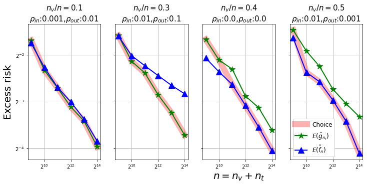
(a) HPO with $|\Lambda|=36$

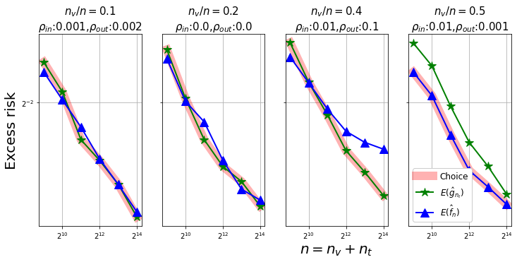
(b) HPO with $|\Lambda|=18$

Figure 2: Empirical utility of Heuristic 3.1 for data dependent choice of $\tilde{f}_{n,\hat{\lambda}}$ vs $\tilde{\mathrm{g}}_{m,\hat{\lambda}}$ with a subset of the varying values of $n,\nicefrac{{\mu}}{{n}},\rho_{\text{{\footnotesize\tt in}}},\rho_{\text{{\footnotesize\tt out}}}$. The vertical axis is the excess risk (lower is better) and the horizontal axis is the total number of available samples $n$. Note the logscale on both axes. See Appendix D.1 for results on all combinations.

We evaluate our heuristics on HPO with neural network configurations. We consider neural networks to have better control over $\rho_{\text{{\footnotesize\tt in}}}$ in the ERM. We chose a synthetic data distribution to have control over the experiment and to be able to generate fresh large samples to accurately estimate the true risks of the different models (as opposed to our results in §2.2 which were based on the true risk estimated on a limited test set). This is common practice when empirically studying theoretical bounds on various statistical quantities (see for example (Rodriguez et al., 2009)). This also allows us to perform the empirical evaluation under various setting (such as different $n$, $\mu$, $\Lambda$). We set the Bayes optimal risk $E(f^{\star})=0$. We consider two HPO problems with grid-search: (a) one with 36 HP configurations ($L=|\Lambda|=36$), and (b) another with 18 HP configurations ($L=|\Lambda|=18$). The data generation and the HP search spaces are detailed in Appendix C. We estimate the true risk $E(f)$ of any model $f$ with a separate large test sample from the synthetic data distribution. We consider sample sizes $n\in[2^{9},2^{14}]$ and different values for $\nicefrac{{\mu}}{{n}}\in[0.1,0.5]$ with $m$ set to $(n-\mu)$. Each ERM involves 5 restarts and the results are averaged over 10 trials (corresponding to different samples from the same distribution). We set the failure probability $\delta=0.05$.

We first evaluate the practical utility of Heuristic 3.1, which tries to balance the gain from utilizing the full data for obtaining $\tilde{f}_{n,\hat{\lambda}}$ and the associated statistical cost of an additional ERM. Figure 2 compares this “Choice” based on Heuristic 3.1 (thick translucent red line) to $\tilde{f}_{n,\hat{\lambda}}$ & $\tilde{\mathrm{g}}_{m,\hat{\lambda}}$ (solid blue $\blacktriangle$ & green $\star$ respectively) for a subset of the combinations of $\rho_{\text{{\footnotesize\tt in}}}$, $\rho_{\text{{\footnotesize\tt out}}}$ and $\nicefrac{{\mu}}{{n}}$, showing the excess risk on the vertical axis as the number of samples $n$ is increased. The results indicate that, depending on $\Lambda$, $\rho_{\text{{\footnotesize\tt in}}}$, $\rho_{\text{{\footnotesize\tt out}}}$ and $\nicefrac{{\mu}}{{n}}$, $\tilde{\mathrm{g}}_{m,\hat{\lambda}}$ might be preferable to $\tilde{f}_{n,\hat{\lambda}}$ and vice versa – one is not always better than the other (as we also highlighted in §2.2), and always selecting $\tilde{f}_{n,\hat{\lambda}}$ (as done in practice) leaves room for improvement. In both types of cases, Heuristic 3.1 is able to select the better options in many cases – the proposed heuristic provides a data-driven way of selecting between $\tilde{f}_{n,\hat{\lambda}}$ and $\tilde{\mathrm{g}}_{m,\hat{\lambda}}$. We provide the full set of results for all considered values of $\rho_{\text{{\footnotesize\tt in}}}$, $\rho_{\text{{\footnotesize\tt out}}}$, $\nicefrac{{\mu}}{{n}}$ for both HPO problems in Appendix D.1. There are cases where the heuristic does not make the right choice, which indicates that there is room for improvement.

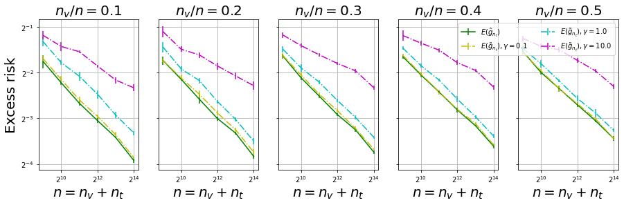
(a) Excess-risk from Heuristic 3.2.

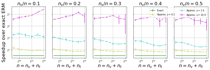
(b) Speedup from Heuristic 3.2.

Figure 3: Empirical validation of the utility of Heuristic 3.2 for data-dependent choice of $\rho_{\text{{\footnotesize\tt in}}}$

To demonstrate the practical utility of the proposed Heuristic 3.2, we continue with the aforementioned HP selection problem over 36 neural network configurations on a synthetic classification data. We consider three choices $\gamma\in\{0.1,1,10\}$ in Heuristic 3.2. We set $\delta=0.05$ and consider different values of $n$ and $\nicefrac{{\mu}}{{n}}$. Figure 3 compares the performance of the HPO with exact ERM using $\hat{\mathrm{g}}_{m,\lambda},\lambda\in\Lambda$ to the HPO with approximate ERM for different $\rho_{\text{{\footnotesize\tt in}}}$ using $\tilde{\mathrm{g}}_{m,\lambda}$ instead. In Figure 3(a), we compare the excess risk incurred from approximate ERM with the data dependent choice of $\rho_{\text{{\footnotesize\tt in}}}$ compared to exact ERM. We see that $\gamma=0.1$ leads to a sufficiently small $\rho_{\text{{\footnotesize\tt in}}}$ that matches the predictive performance of exact ERM. Any smaller approximation $\rho_{\text{{\footnotesize\tt in}}}$ would not improve the excess risk. The results also indicate that $\gamma=10$ leads to a $\rho_{\text{{\footnotesize\tt in}}}$ where the optimization error dominates the excess risk, implying that $\rho_{\text{{\footnotesize\tt in}}}$ should be reduced if possible. Figure 3(b) presents the computational speedups obtained for the corresponding data-dependent choices of $\rho_{\text{{\footnotesize\tt in}}}$ – we see that we can get a $2\times$ speedup over exact ERM without any degradation in excess risk with $\gamma=0.1$ while obtaining around $4-8\times$ speedup with slight degradation in performance with $\gamma=1$. These results provide empirical evidence for the practical utility of the proposed Heuristic 3.2 obtained from Theorem 3.1 – the proposed heuristic provides a data driven way of setting the ERM approximation tolerance in HPO.

4 Related work

While the use of smaller number of samples $m<n$ to select the HP $\hat{\lambda}$ is often recognized in practice, and leads to the final model being learned via ERM on $\mathcal{F}_{\hat{\lambda}}$ using all $n$ samples, no theoretical guarantees exist for this process. We explicitly study this situation, introducing the hold-in risk $\mathcal{E}_{\text{{\footnotesize{\tt hin}}}}$, and provide a novel guarantee for such a procedure in Theorem 3.2. Kearns (Kearns, 1996) studies the interaction between the approximation and estimation risks, and under certain assumptions and restricted class of functions, proposes ways for selecting the sizes of the training and held-out splits $m$ and $\mu$ in an informed manner. To account for the fact that some of the training data is “wasted” as the held-out set, Blum et al. (Blum et al., 1999) propose two different ways of retaining the Hoeffding bounds of the error estimate on the held-out set while still being able to utilize the full training data to train models employed at test time. These techniques are ways of modifying the standard CV.

In addition to the above, there are various theoretical analyses focusing on various aspects of the CV process such as obtaining tight variance estimates for the $k$-fold CV score of any given HP $\lambda\in\Lambda$ (Nadeau and Bengio, 1999, 2003; Rodriguez et al., 2009; Markatou et al., 2005). These results are complementary to ours and could be used to extend our current results (for the single training/validation split based CV) to $k$-fold CV, with the variance estimates for the $k$-fold CV metrics involved in the data-driven heuristics. We will pursue this in future research. However, note that these existing results do not directly help us obtain tighter excess risk bounds or allow comparison between models $\tilde{\mathrm{g}}_{m,\hat{\lambda}}$ (used during the HPO) and the final deployed model $\tilde{f}_{n,\hat{\lambda}}$ or provide any intuition regarding the choices for $\rho_{\text{{\footnotesize\tt in}}}$ and $\rho_{\text{{\footnotesize\tt out}}}$, which are the main questions (Q1a, Q1b, Q2a, Q2b) we study.

Finally, as we discussed in §1, HPO has been widely studied over the last decade. However, the questions we focus on are complementary to any specific HPO scheme. We do not focus on how the HP was found (with any specific HPO scheme such Bayesian Optimization (Shahriari et al., 2016)), but rather on (i) the ERM involved in the evaluation of any HP during the HPO, and (ii) the ERM involved in the final deployment after an HP is selected. Our Heuristic 3.2 allows us to speed up any HPO scheme without any additional excess risk, and our Heuristics 3.1 and B.1 allow us to improve the predictive performance of the deployed model for the HP $\hat{\lambda}$ selected via any HPO scheme. “Multi-fidelity” HPO schemes (Li et al., 2018; Jamieson and Talwalkar, 2016; Sabharwal et al., 2016; Klein et al., 2017; Falkner et al., 2018) significantly improve the computational efficiency by adaptively setting either the training set size $m<n$ or the optimization approximation $\rho_{\text{{\footnotesize\tt in}}}$ on a per-HP basis instead of using a single value of $m$ or $\rho_{\text{{\footnotesize\tt in}}}$ for all $\lambda\in\Lambda$. This is quite different from our proposed Heuristic 3.2 and the excess risk introduced by this adaptive strategy is not studied to the best of our knowledge. We wish to extend our tradeoff analysis to multi-fidelity HPO in future work. Meta-learning is another way of improving the efficiency of the HPO process (Vanschoren, 2018), and has been used in some AutoML toolkits (Feurer et al., 2015, 2020). Recently, some theoretical guarantees have been established for such meta-learning based HPO (Ram, 2022), and we also wish to extend our tradeoff analysis to such meta-learning based HPO. Note that the proposed Heuristics 3.1 and B.1 is still beneficial in both the above situations (multi-fidelity and meta-learning).

5 Conclusions

Our contributions focus on aspects of CV based HPO – we explore how to leverage the different tradeoffs in the excess risk to make various practical decisions in the HPO process in a data-driven manner. We use the novel excess risk decomposition and theoretical analyses to answer the two questions in CV-based HPO: (1) When is the process of training the model on all the data after the HPO beneficial and can we choose between the two in a data driven manner? (Q1a, Q1b) (2) At what level should we set the tolerance of the optimization involved in model training during HPO? (Q2a, Q2b). The ideas can be utilized by data science practitioners as well as by automated data science systems.

Appendix A Detailed Proofs

We will make sure of this standard result:

Theorem A.1.

([Bartlett and Mendelson, 2002]) Consider conditions and notations of Theorem 3.1. Then for any $\delta>0$, with probability at least $1-\delta$, the following is true:

$$\sup_{f\in\mathcal{F}_{\lambda}}\left|E_{n}(f)-E(f)\right|\leq 4\,\beta\,\mathcal{R}_{n}(\mathcal{F}_{\lambda})+2\,B\,\sqrt{\nicefrac{{\log(1/\delta)}}{{2n}}}.$$ (11)

where $\mathcal{R}_{n}(\mathcal{F}_{\lambda})$ is the Radamacher complexity of $\mathcal{F}_{\lambda}$.

A.1 Proof of Theorem 3.1

Proof.

(Theorem 3.1) By definition of $\mathcal{F}_{\hat{\lambda}}$, for any $\lambda\in\Lambda$ and $\delta^{\prime}>0$, we have the following relationships:

$$E(\tilde{\mathrm{g}}_{m,\hat{\lambda}}) \stackrel{{\scriptstyle(a)}}{{\leq}}E^{v}_{\mu}(\tilde{\mathrm{g}}_{m,\hat{\lambda}})+B\sqrt{\log(1/\delta^{\prime})/2\mu}\qquad\text{ w.p. }\geq 1-\delta^{\prime}$$ (12)

$$\stackrel{{\scriptstyle(b)}}{{\leq}}E^{v}_{\mu}(\tilde{\mathrm{g}}_{m,\lambda})+B\sqrt{\log(1/\delta^{\prime})/2\mu}$$ (13)

$$\stackrel{{\scriptstyle(c)}}{{\leq}}E(\tilde{\mathrm{g}}_{m,\lambda})+2B\sqrt{\log(1/\delta^{\prime})/2\mu}\qquad\text{ w.p. }\geq 1-\delta^{\prime},$$ (14)

where $(a)$ and $(c)$ are obtained from an application of Hoeffding’s inequality while $(b)$ is obtained from the definition of $\hat{\lambda}$ in (4) as the minimizer of $E_{\mu}^{v}(\tilde{\mathrm{g}}_{m,\lambda})$. For any $\mathcal{F}_{\lambda},\lambda\in\Lambda$, we have the following:

$$E(\tilde{\mathrm{g}}_{m,\lambda}) \stackrel{{\scriptstyle(d)}}{{\leq}}E_{m}(\tilde{\mathrm{g}}_{m,\lambda})+4\beta\mathcal{R}_{m}(\mathcal{F}_{\lambda})+2B\sqrt{\log(1/\delta^{\prime})/2m}\qquad\text{ w.p. }\geq 1-\delta^{\prime}$$

$$\stackrel{{\scriptstyle(e)}}{{\leq}}E_{m}(\hat{\mathrm{g}}_{m,\lambda})+\rho_{\text{{\footnotesize\tt in}}}+4\beta\mathcal{R}_{m}(\mathcal{F}_{\lambda})+2B\sqrt{\log(1/\delta^{\prime})/2m}$$

$$\stackrel{{\scriptstyle(f)}}{{\leq}}E_{m}(\bar{f}_{\lambda})+\rho_{\text{{\footnotesize\tt in}}}+4\beta\mathcal{R}_{m}(\mathcal{F}_{\lambda})+2B\sqrt{\log(1/\delta^{\prime})/2m}$$

$$\stackrel{{\scriptstyle(g)}}{{\leq}}E(\bar{f}_{\lambda})+\rho_{\text{{\footnotesize\tt in}}}+8\beta\mathcal{R}_{m}(\mathcal{F}_{\lambda})+4B\sqrt{\log(1/\delta^{\prime})/2m}\qquad\text{ w.p. }\geq 1-\delta^{\prime}$$

$$\stackrel{{\scriptstyle(h)}}{{\leq}}E(f^{\star})+\mathcal{E}_{\text{{\footnotesize{\tt app}}}}(\lambda)+\rho_{\text{{\footnotesize\tt in}}}+8\beta\mathcal{R}_{m}(\mathcal{F}_{\lambda})+4B\sqrt{\log(1/\delta^{\prime})/2m},$$ (15)

where $(d)$ and $(g)$ are obtained by Theorem A.1, $(e)$ is obtained from the problem definition (4) for the approximate ERM solution, $(f)$ is obtained from the definition of $\hat{\mathrm{g}}_{m,\lambda}$ as the ERM solution for any class $\mathcal{F}_{\lambda}$, and $(h)$ is a simple application of the definition of the approximation risk $\mathcal{E}_{\text{{\footnotesize{\tt app}}}}(\lambda)$ of any class $\mathcal{F}_{\lambda}$.

Since the above holds for any $\lambda\in\Lambda$, putting (14) and (15) together using the union bound with $\delta^{\prime}=\delta/(2+2|\Lambda|)=\delta/2(L+1)$ and minimizing over $\lambda\in\Lambda$ gives us the desired result in (8) with a failure probability of at most $\delta$. ∎

A.2 Proof of Theorem 3.2

Proof.

(Theorem 3.2) By definition of $\mathcal{F}_{\hat{\lambda}}$ and $\tilde{f}_{n,\hat{\lambda}}\in\mathcal{F}_{\hat{\lambda}}$, we have the following with an application of Theorem A.1 w.p. $\geq 1-\delta^{\prime}$:

$$E(\tilde{f}_{n,\hat{\lambda}})\leq E_{n}(\tilde{f}_{n,\hat{\lambda}})+4\beta\mathcal{R}_{n}(\mathcal{F}_{\hat{\lambda}})+2B\sqrt{\log(1/\delta^{\prime})/2n}$$ (16)

Now from the problem definition and the definition of $\mathcal{I}_{n,m}^{\hat{\lambda}}$:

$$E_{n}(\tilde{f}_{n,\hat{\lambda}}) =E_{n}(\tilde{\mathrm{g}}_{m,\hat{\lambda}})-\mathcal{I}_{n,m}^{\hat{\lambda}}(\rho_{\text{{\footnotesize\tt in}}},\rho_{\text{{\footnotesize\tt out}}})$$ (17)

However, we have an alternate relationship as follows:

$$E_{n}(\tilde{f}_{n,\hat{\lambda}}) \stackrel{{\scriptstyle(a)}}{{\leq}}E_{n}(\hat{f}_{n,\hat{\lambda}})+\rho_{\text{{\footnotesize\tt out}}}$$ (18)

$$\stackrel{{\scriptstyle(b)}}{{=}}E_{n}(\hat{\mathrm{g}}_{m,\hat{\lambda}})-\mathcal{I}_{n,m}^{\hat{\lambda}}(0,0)+\rho_{\text{{\footnotesize\tt out}}}$$ (19)

$$\stackrel{{\scriptstyle(c)}}{{\leq}}E_{n}(\tilde{\mathrm{g}}_{m,\hat{\lambda}})+\frac{\mu}{n}B-\mathcal{I}_{n,m}^{\hat{\lambda}}(0,0)+\rho_{\text{{\footnotesize\tt out}}},$$ (20)

where $(a)$ is from the definition of the approximate ERM solution $\tilde{f}_{n,\hat{\lambda}}$ and the exact ERM solution $\hat{f}_{n,\hat{\lambda}}$, $(b)$ is obtained from the definition of $\mathcal{I}_{n,m}^{\hat{\lambda}}(0,0)$ in the statement of the theorem, and $(c)$ is from the definition of $\hat{\mathrm{g}}_{m,\hat{\lambda}}$ as the minimizer of $E_{m}(\cdot)$ in $\mathcal{F}_{\hat{\lambda}}$ and the fact that, for any $f$, $E_{n}(f)=(m/n)E_{m}(f)+(\mu/n)E_{\mu}(f)$ and the loss $\ell$ is bounded by $B$.

Putting (17) and (20) gives us:

$$\begin{split}E_{n}(\tilde{f}_{n,\hat{\lambda}})\leq E_{n}(\tilde{\mathrm{g}}_{m,\hat{\lambda}})-\underbrace{\max\left\{\mathcal{I}_{n,m}^{\hat{\lambda}}(\rho_{\text{{\footnotesize\tt in}}},\rho_{\text{{\footnotesize\tt out}}}),\quad\mathcal{I}_{n,m}^{\hat{\lambda}}(0,0)-\frac{\mu}{n}B-\rho_{\text{{\footnotesize\tt out}}}\right\}}_{:=\bar{\mathcal{I}}\text{ in Theorem~{}\ref{thm:ehpo-bnd-md}}}.\end{split}$$

Using above in (16), we get the following relationships:

$$E(\tilde{f}_{n,\hat{\lambda}}) \leq E_{n}(\tilde{\mathrm{g}}_{m,\hat{\lambda}})-\bar{\mathcal{I}}+4\beta\mathcal{R}_{n}(\mathcal{F}_{\hat{\lambda}})+2B\sqrt{\log(1/\delta^{\prime})/2n}\qquad\text{ w. p. }\geq 1-\delta^{\prime}$$

$$\leq E(\tilde{\mathrm{g}}_{m,\hat{\lambda}})-\bar{\mathcal{I}}+8\beta\mathcal{R}_{n}(\mathcal{F}_{\hat{\lambda}})+4B\sqrt{\log(1/\delta^{\prime})/2n}\qquad\text{ w. p. }\geq 1-2\delta^{\prime},$$

where the last inequality is an application of Theorem A.1 on $\tilde{\mathrm{g}}_{n,\hat{\lambda}}\in\mathcal{F}_{\hat{\lambda}}$. Combining (A.2) with (14) (which holds w.p. $\geq 1-2\delta^{\prime}$) and (15) (which holds w.p. $\geq 1-2\delta^{\prime}$ for each $\lambda\in\Lambda$) and applying the union bound over all $\lambda\in\Lambda$, we have

$$E(\tilde{f}_{n,\hat{\lambda}})-E(\tilde{\mathrm{g}}_{m,\hat{\lambda}})$$

$$\quad\leq-\bar{\mathcal{I}}+8\beta\mathcal{R}_{n}(\mathcal{F}_{\hat{\lambda}})+4B\sqrt{\nicefrac{{\log(\nicefrac{{1}}{{\delta^{\prime}}})}}{{2n}}} =-\bar{\mathcal{I}}+8\beta\mathcal{R}_{n}(\mathcal{F}_{\hat{\lambda}})+B^{\prime}(\nicefrac{{2}}{{\sqrt{2n}}})\quad\text{ w.p.}\geq 1-2\delta^{\prime},$$ (21)

We also know that for all $\lambda\not=\hat{\lambda}\in\Lambda$,

$$E(\tilde{\mathrm{g}}_{m,\hat{\lambda}})-E(\tilde{\mathrm{g}}_{m,\lambda}) \leq 2B\sqrt{\nicefrac{{\log(\nicefrac{{1}}{{\delta^{\prime}}})}}{{2\mu}}}=B^{\prime}(\nicefrac{{1}}{{\sqrt{2\mu}}})\qquad\text{ w.p. }\geq 1-2\delta^{\prime},$$

$$E(\tilde{\mathrm{g}}_{m,\lambda})-E(f^{\star}) \leq\min_{\lambda\in\Lambda}\left[\mathcal{E}_{\text{{\footnotesize{\tt app}}}}(\lambda)+\rho_{\text{{\footnotesize\tt in}}}+8\beta\mathcal{R}_{m}(\mathcal{F}_{\lambda})\right]+4B\sqrt{\frac{\log(\nicefrac{{1}}{{\delta^{\prime}}})}{2m}}$$

$$=\min_{\lambda\in\Lambda}\left[\mathcal{E}_{\text{{\footnotesize{\tt app}}}}(\lambda)+\rho_{\text{{\footnotesize\tt in}}}+8\beta\mathcal{R}_{m}(\mathcal{F}_{\lambda})\right]+B^{\prime}\left(\frac{2}{\sqrt{2m}}\right)$$

w.p. $\geq 1-2L\delta^{\prime}$ where we replace $2B\sqrt{\log(1/\delta^{\prime})}$ with $B^{\prime}$.

Putting the above together, we get the upperbound for $\mathcal{E}=E(\tilde{f}_{n,\hat{\lambda}})-E(f^{\star})$ in the statement of the claim with probability at least $1-(2+2L+2)\delta^{\prime}=1-2(L+2)\delta^{\prime}=1-\delta$ by setting $\delta^{\prime}=\delta/(2(L+2))$. ∎

A.3 Tighter version of Theorem 3.1.

Theorem A.2 (Adapted from Boucheron et al. [2005], Thm 8.16).

Consider the conditions and notations of Theorem 3.1. If we further assume that there exists a non-decreasing function $w:\mathbb{R}_{+}\to\mathbb{R}_{+}$ with $w(x)/\sqrt{x}$ non-increasing for $x\in\mathbb{R}_{+}$ such that, for any function $f$, $\sqrt{\text{Var}\left[|f-f^{\star}|\right]}\leq w\left(E(f)-E(f^{\star})\right)$, then the excess risk of $\tilde{\mathrm{g}}_{m,\hat{\lambda}}$ can be bounded from above as:

$$\begin{split}\mathcal{E}\leq&\min_{\theta\in(0,1)}\left(1+\theta\right)\left(\min_{\lambda\in\Lambda}\left\{8\cdot\beta\cdot\mathcal{R}_{n}(\mathcal{F}_{\lambda})+\mathcal{E}_{\text{{\footnotesize{\tt app}}}}(\lambda)\right\}+\rho_{\text{{\footnotesize\tt in}}}\right.\\ &\qquad\qquad\qquad\quad\left.+2B\cdot\sqrt{\frac{2\log((2L+1)/\delta)}{m}}+4\cdot B\cdot\log\frac{2L+1}{\delta}\left(\frac{\tau^{*}(\mu)}{\theta}+\frac{2}{3\mu}\right)\right),\end{split}$$

where $\tau^{*}(n)=\min\{x>0:w(x)=x\sqrt{n}\}$ for any $n>0$.

Proof.

For any $\lambda\in\Lambda$ and some $\delta^{\prime}>0$, we have the following from Berstein’s inequality:

$$E(\tilde{\mathrm{g}}_{m,\lambda})-E(f^{\star}) \leq E_{\mu}^{v}(\tilde{\mathrm{g}}_{m,\lambda})-E_{\mu}^{v}(f^{\star})+w(E(\tilde{\mathrm{g}}_{m,\lambda})-E(f^{\star}))\sqrt{\frac{2\log(1/\delta^{\prime})}{\mu}}+\frac{4\log(1/\delta^{\prime})}{3\mu}.$$ (22)

with probability at least $1-\delta^{\prime}$.

Let $\bar{\lambda}=\arg\min_{\lambda\in\Lambda}E(\tilde{\mathrm{g}}_{m,\lambda})$. Then again applying Berstein’s inequality with $\delta^{\prime}>0$, we have

$$E(f^{\star})-E(\tilde{\mathrm{g}}_{m,\bar{\lambda}}) \leq E_{\mu}^{v}(f^{\star})-E_{\mu}^{v}(\tilde{\mathrm{g}}_{m,\bar{\lambda}})+w(E(\tilde{\mathrm{g}}_{m,\bar{\lambda}})-E(f^{\star}))\sqrt{\frac{2\log(1/\delta^{\prime})}{\mu}}+\frac{4\log(1/\delta^{\prime})}{3\mu}.$$ (23)

with probability at least $1-\delta^{\prime}$.

Combining the above two inequalities over all $\lambda\in\Lambda$, using the definition of $\tilde{\mathrm{g}}_{m,\hat{\lambda}}$ as the minimizer of $E_{\mu}^{v}(\cdot)$, and the non-decreasing nature of $w(\cdot)$ gives us the following with probability at least $1-(L+1)\delta^{\prime}$:

$$E(\tilde{\mathrm{g}}_{m,\hat{\lambda}})-E(\tilde{\mathrm{g}}_{m,\bar{\lambda}}) \leq 2w(E(\tilde{\mathrm{g}}_{m,\hat{\lambda}})-E(f^{\star}))\sqrt{\frac{2\log(1/\delta^{\prime})}{\mu}}+\frac{8\log(1/\delta^{\prime})}{3\mu}.$$ (24)

Given $\tau^{*}(\mu)$ as defined in the statement of the claim, $w(\tau^{*}(\mu))=\tau^{*}(\mu)\sqrt{\mu}$. Now, either $E(\tilde{\mathrm{g}}_{m,\hat{\lambda}})-E(f^{\star})<\tau^{*}(\mu)$. Or $E(\tilde{\mathrm{g}}_{m,\hat{\lambda}})-E(f^{\star})\geq\tau^{*}(\mu)$, which gives us the following:

$$\frac{w(E(\tilde{\mathrm{g}}_{m,\hat{\lambda}})-E(f^{\star}))}{\sqrt{E(\tilde{\mathrm{g}}_{m,\hat{\lambda}})-E(f^{\star})}}\stackrel{{\scriptstyle(a)}}{{\leq}}\frac{w(\tau^{*}(\mu))}{\sqrt{\tau^{*}(\mu)}}\stackrel{{\scriptstyle(b)}}{{=}}\sqrt{\tau^{*}(\mu)}\sqrt{\mu},$$ (25)

where $(a)$ comes from the assumptions that $w(x)/\sqrt{x}$ is non-increasing in $x\in\mathbb{R}_{+}$ and $(b)$ comes from the definition of $\tau^{*}(\mu)$. Using the above in (24) gives us:

$$E(\tilde{\mathrm{g}}_{m,\hat{\lambda}})-E(\tilde{\mathrm{g}}_{m,\bar{\lambda}}) \leq 2\sqrt{E(\tilde{\mathrm{g}}_{m,\hat{\lambda}})-E(f^{\star})}\sqrt{\frac{2\log(1/\delta^{\prime})}{\mu}}\sqrt{\tau^{*}(\mu)}+\frac{8\log(1/\delta^{\prime})}{3\mu}$$ (26)

$$\leq\frac{\theta}{2}\left(E(\tilde{\mathrm{g}}_{m,\hat{\lambda}})-E(f^{\star})\right)+\frac{8}{2\theta}\log(1/\delta^{\prime})\tau^{*}(\mu)+\frac{8\log(1/\delta^{\prime})}{3\mu}.$$ (27)

where we utilize the fact that the arithmetic mean is greater than or equal to the geometric mean for some $\theta\in(0,1)$.

Then we can get, w.p. $\geq 1-(L+1)\delta^{\prime}$:

$$\left(E(\tilde{\mathrm{g}}_{m,\hat{\lambda}})-E(f^{\star})\right)(1-\theta/2) \leq E(\tilde{\mathrm{g}}_{m,\bar{\lambda}})-E(f^{\star})+4\log(1/\delta^{\prime})\left(\frac{\tau^{*}(\mu)}{\theta}+\frac{2}{3\mu}\right).$$ (28)

Now we have the following by definition of $\bar{\lambda}$ and $\tilde{\mathrm{g}}_{m,\bar{\lambda}}\in\mathcal{F}_{\bar{\lambda}}$:

$$E(\tilde{\mathrm{g}}_{m,\bar{\lambda}})-E(f^{\star}) =\min_{\lambda\in\Lambda}\left(E(\tilde{\mathrm{g}}_{m,\lambda})-E(f^{\star})\right)$$ (29)

$$\stackrel{{\scriptstyle(c)}}{{\leq}}\min_{\lambda\in\Lambda}\left(E(\bar{f}_{\lambda})-E(f^{\star})+2\sup_{f\in\mathcal{F}_{\lambda}}\left|E(f)-E_{m}(f)\right|+\rho_{\text{{\footnotesize\tt in}}}\right)$$ (30)

$$\stackrel{{\scriptstyle(d)}}{{\leq}}\min_{\lambda\in\Lambda}\left(\mathcal{E}_{\text{{\footnotesize{\tt app}}}}(\lambda)+8\cdot\beta\cdot\mathcal{R}_{n}(\mathcal{F}_{\lambda})+2B\cdot\sqrt{\frac{2\log(1/\delta^{\prime})}{m}}+\rho_{\text{{\footnotesize\tt in}}}\right)\quad\text{ w.p. }\geq 1-L\delta^{\prime}$$ (31)

where $(d)$ is obtained from the application of Theorem A.1 on each $\lambda\in\Lambda$, and $(c)$ is obtained as follows:

$$E(\tilde{\mathrm{g}}_{m,\lambda}) \leq E_{m}(\tilde{\mathrm{g}}_{m,\lambda})+\sup_{f\in\mathcal{F}_{\lambda}}|E(f)-E_{m}(f)|$$ (32)

$$\leq E_{m}(\hat{\mathrm{g}}_{m,\lambda})+\rho_{\text{{\footnotesize\tt in}}}+\sup_{f\in\mathcal{F}_{\lambda}}|E(f)-E_{m}(f)|$$ (33)

$$\leq E_{m}(\bar{f}_{\lambda})+\rho_{\text{{\footnotesize\tt in}}}+\sup_{f\in\mathcal{F}_{\lambda}}|E(f)-E_{m}(f)|$$ (34)

$$\leq E(\bar{f}_{\lambda})+\rho_{\text{{\footnotesize\tt in}}}+2\sup_{f\in\mathcal{F}_{\lambda}}|E(f)-E_{m}(f)|.$$ (35)

Combining (28) and (31), setting $\delta^{\prime}=\delta/(2L+1)$ and noting that $(1-\theta/2)^{-1}\leq(1+\theta)$ for $\theta\in(0,1)$ gives us the statement of the claim. ∎

Appendix B Data-driven heuristic for $\rho_{\text{{\footnotesize\tt out}}}$

While we have a very precise way of setting $\rho_{\text{{\footnotesize\tt in}}}$ given the theoretical result, the choice of $\rho_{\text{{\footnotesize\tt out}}}$ is somewhat more involved. Based on Theorem 3.2, we can utilize the following heuristic to set $\rho_{\text{{\footnotesize\tt out}}}$:

Heuristic B.1.

Assuming that $\rho_{\text{{\footnotesize\tt out}}}$ can be iteratively reduced during the approximate ERM for $\tilde{f}_{n,\hat{\lambda}}$, based on the terms in Theorem 3.2 and a given $\rho_{\text{{\footnotesize\tt in}}}$, we propose the following iterative scheme to set $\rho_{\text{{\footnotesize\tt out}}}$ with scaling parameters $\nu\in(0,1),\gamma>0$: For $T>0$, we iteratively reduce $\rho_{\text{{\footnotesize\tt out}}}$ as

$$\begin{split}&\rho_{\text{{\footnotesize\tt out}}}^{(T+1)}\leftarrow\nu\cdot\rho_{\text{{\footnotesize\tt out}}}^{(T)}\quad\text{ if }\ \ \Gamma(\rho_{\text{{\footnotesize\tt out}}}^{(T-1)})-\Gamma(\rho_{\text{{\footnotesize\tt out}}}^{(T)})>\gamma\cdot\kappa\\ &\text{exit approx. ERM}\quad\text{ otherwise},\end{split}$$ (36)

where $\Gamma(\rho_{\text{{\footnotesize\tt out}}}):=\mathcal{I}_{n,m}^{\hat{\lambda}}(\rho_{\text{{\footnotesize\tt in}}},\rho_{\text{{\footnotesize\tt out}}})$, $\rho_{\text{{\footnotesize\tt out}}}^{(0)}\leftarrow\rho_{\text{{\footnotesize\tt in}}}$, and $\kappa:=\rho_{\text{{\footnotesize\tt in}}}+B\sqrt{2\log(\nicefrac{{2(L+2)}}{{\delta}})}(\nicefrac{{2}}{{\sqrt{n}}}+\nicefrac{{2}}{{\sqrt{m}}}+\nicefrac{{1}}{{\sqrt{\mu}}})$.

This heuristic leverages the fact that the empirical risk improvement $\mathcal{I}_{n,m}^{\hat{\lambda}}(\rho_{\text{{\footnotesize\tt in}}},\rho_{\text{{\footnotesize\tt out}}})$ will increase as $\rho_{\text{{\footnotesize\tt out}}}$ is reduced up until a point, and the excess risk of $\tilde{f}_{n,\hat{\lambda}}$ is closely tied to this empirical risk improvement – more improvement implies better excess risk. Heuristic B.1 tries to balance any increase in this empirical risk improvement with the other (computable) terms, denoted as $\kappa$, in the excess risk bound in (9) – we stop reducing $\rho_{\text{{\footnotesize\tt out}}}$ when the increase in the empirical risk improvement $\Gamma(\rho_{\text{{\footnotesize\tt out}}}^{(T-1)})-\Gamma(\rho_{\text{{\footnotesize\tt out}}}^{(T)})$ is an order of magnitude below $\kappa$, at which point, other terms dominate the excess risk. Heuristics 3.2 and B.1 are our answers to Q2b.

Heuristic B.1 just presents a way to identify when $\rho_{\text{{\footnotesize\tt out}}}$ is sufficiently small in terms of statistical performance while being able to gain computationally when we are able to approximate the ERM in an iterative manner and progressively decrease $\rho_{\text{{\footnotesize\tt out}}}$.

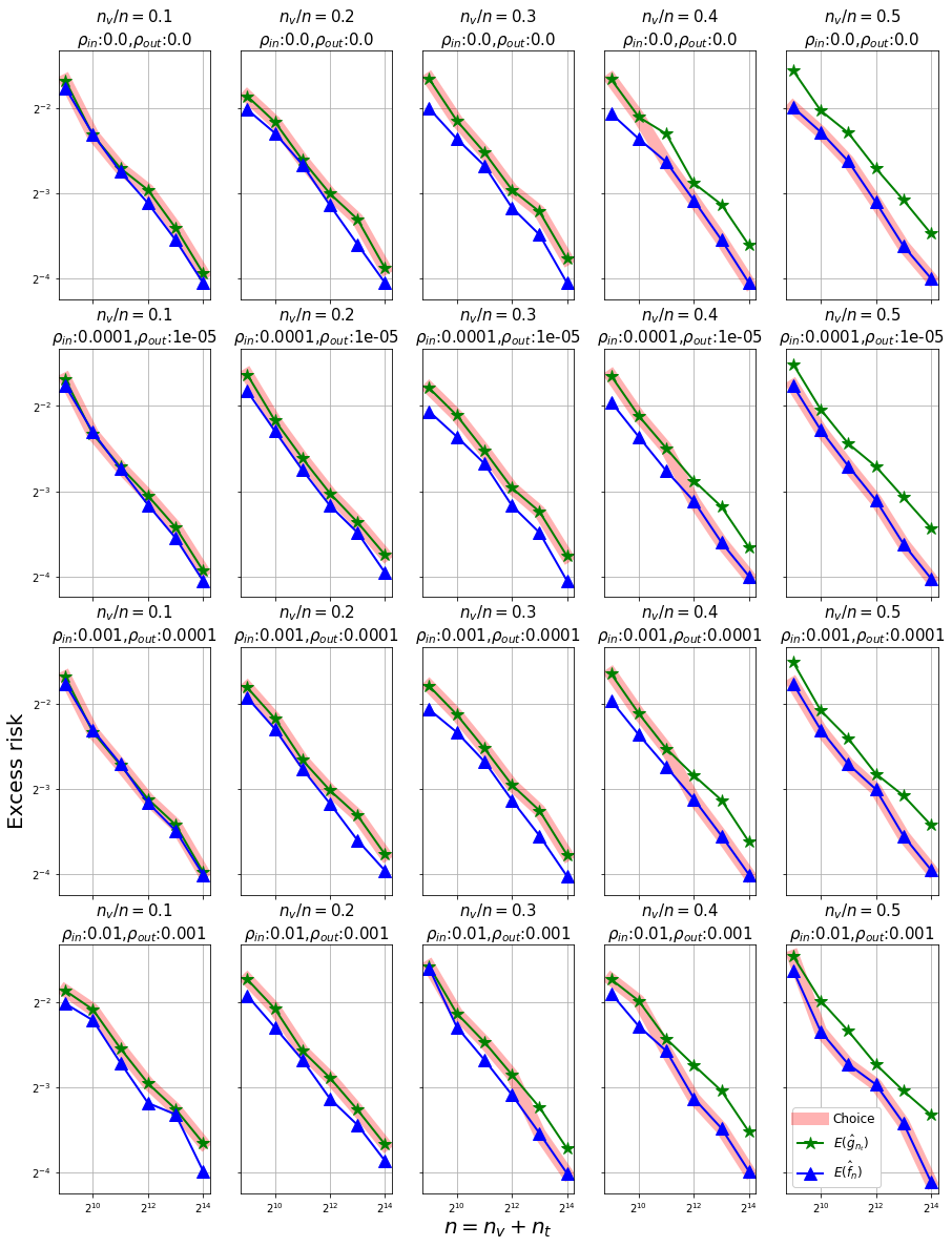
(a) $\rho_{\text{{\footnotesize\tt out}}}=\nicefrac{{\rho_{\text{{\footnotesize\tt in}}}}}{{10}}$

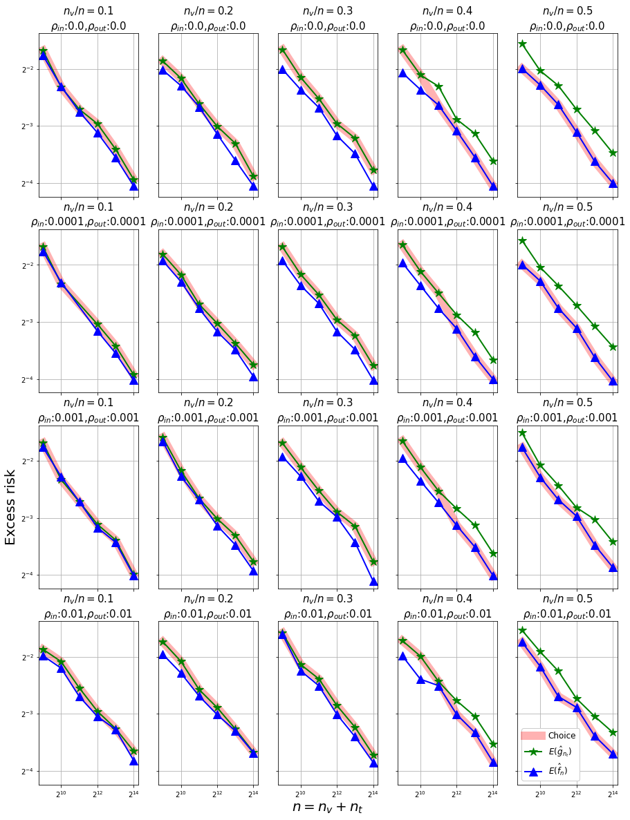
(b) $\rho_{\text{{\footnotesize\tt out}}}=\rho_{\text{{\footnotesize\tt in}}}$

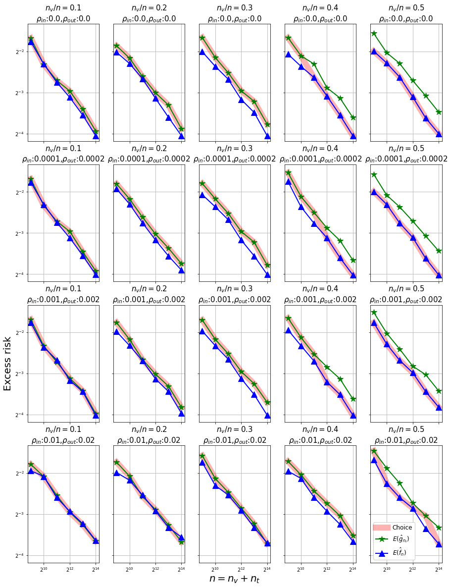
(c) $\rho_{\text{{\footnotesize\tt out}}}=2\cdot\rho_{\text{{\footnotesize\tt in}}}$

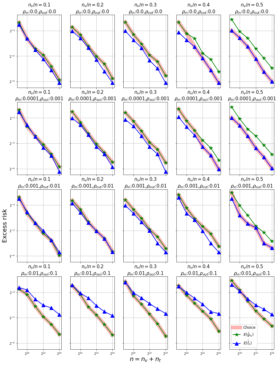
(d) $\rho_{\text{{\footnotesize\tt out}}}=10\cdot\rho_{\text{{\footnotesize\tt in}}}$

Figure 4: Excess-risk of data-dependent choice between $\tilde{f}_{n,\hat{\lambda}}$ and $\tilde{\mathrm{g}}_{n,\hat{\lambda}}$ based on Heuristic 3.1 for $\rho_{\text{{\footnotesize\tt in}}}\in\{0.0001,0.001,0.01,0.1\}$ and search space with $|\Lambda|=36$. Please magnify to view in detail.

Appendix C Empirical evaluation details

Synthetic data generation.

The binary classification data is generated using the make_classification function [Guyon, 2003] in scikit-learn [Pedregosa et al., 2011]. We ensure that the classes are not overlapping and there is no label noise, ensuring that the Bayes optimal risk $E(f^{\star})=0$.

Neural network HP search space.

We consider two different $\Lambda$s for a fully connected neural network, with (i) depth $\in\{1,2,3\}$, (ii) number of neurons in each layer $\in\{10,100\}$, (iii) initial SGD learning rate $\in\{0.01,0.1\}$, (iv) SGD batch size $\in\{8,32,128\}$. The implementation is in PyTorch [Paszke et al., 2019]. For one problem we consider 36 configurations (that is $L=|\Lambda|=36$), and for another, we consider 18 configurations (that is $L=|\Lambda|=18$).

LightGBM HP search space.

We use the following search space for theLGBMClassifier from LightGBM [Ke et al., 2017] with RandomizedSearchCV from scikit-learn: (i) learning rate $\in[0.01,0.4]$, (ii) number of trees $\in[100,5000]$, (iii) number of leaves per tree $\in[6,50]$, (iv) minimum samples in a child node $\in[100,500]$, (v) minimum weight in a child node $\in[10^{-5},10^{4}]$, (vi) sub-sampling rate $\in[.1,.9]$, (vii) maximum depth per tree $\in[-1,7]$, (viii) column sub-sampling rate per tree $\in[.4,.7]$, (ix) $\alpha$ regularization $\in[0,100]$, (x) $\lambda$ regularization $\in[0,100]$.

OpenML data.

The data sets used in this experiment are listed in Table 6 with their OpenML names and IDs. For each data set, we utilize 3 different values of the train-validation split ratio $\nicefrac{{\mu}}{{n}}\in\{0.1,0.2,0.3\}$.

Table 6: Data set name & OpenML ID of all the data sets used with 10 data sets each in the data size range.

# samples	Name (OpenML ID)
1000-4999	kr-vs-kp (3)	credit-g (31)
	sick (38)	spambase (44)
	scene (312)	yeast-ml8 (316)
	fri-c3-1000-25 (715)	fri-c4-1000-100 (718)
	abalone (720)	fri-c4-1000-25 (723)
5000-9999	mushroom (24)	bank8FM (725)
	cpu-small (735)	puma32H (752)
	cpu-act (761)	delta-ailerons (803)
	kin8nm (807)	puma8NH (816)
	delta-elevators (819)	bank32nh (833)
10000-49999	BNG(tic-tac-toe) (137)	electricity (151)
	adult (179)	BNG(breast-w) (251)
	mammography (310)	webdata-wXa (350)
	pol (722)	2dplanes (727)
	ailerons (734)	house-16H (821)
50000-99999	vehicle-sensIT (357)	KDDCup09-app (1111)
	KDDCup09-churn (1112)	KDDCup09-upsell (1114)
	vehicleNorm (1242)	higgs (23512)
	numerai28.6 (23517)	Run-or-walk-info (40922)
	APSFailure (41138)	kick (41162)

Appendix D Extended empirical evaluation

D.1 Further evaluation of Heuristic 3.1

In Figure 2, we demonstrated the empirical utiity of Heuristic 3.1 for a particular choice of $\rho_{\text{{\footnotesize\tt in}}}=\rho_{\text{{\footnotesize\tt out}}}=0$ implying we leverage exact ERM in the inner level of the HPO problem (to obtain $\hat{\mathrm{g}}_{m,\lambda},\lambda\in\Lambda$) and in the final training of the model on the selected HP $\hat{\lambda}$ to obtain $\hat{f}_{n,\hat{\lambda}}\in\mathcal{F}_{\hat{\lambda}}$. In this subsection, we evaluate Heuristic 3.1 for other pre-set values of $\rho_{\text{{\footnotesize\tt in}}}$ and $\rho_{\text{{\footnotesize\tt out}}}$. We start with trying $\rho_{\text{{\footnotesize\tt in}}}\in\{0.0001,0.001,0.01,0.1\}$ and then setting $\rho_{\text{{\footnotesize\tt out}}}$ relative to $\rho_{\text{{\footnotesize\tt in}}}$.

We present the following results for the search space with 36 configuration in Figure 4: (a) Figure 4(a) for $\rho_{\text{{\footnotesize\tt out}}}=\nicefrac{{\rho_{\text{{\footnotesize\tt in}}}}}{{10}}$, (b) Figure 4(b) for $\rho_{\text{{\footnotesize\tt out}}}=\rho_{\text{{\footnotesize\tt in}}}$, (c) Figure 4(c) for $\rho_{\text{{\footnotesize\tt out}}}=2\cdot\rho_{\text{{\footnotesize\tt in}}}$, (d) Figure 4(d) for $\rho_{\text{{\footnotesize\tt out}}}=10\rho_{\text{{\footnotesize\tt in}}}$. We present the following results for the search space with 18 configuration in Figure 5: (a) Figure 5(a) for $\rho_{\text{{\footnotesize\tt out}}}=\nicefrac{{\rho_{\text{{\footnotesize\tt in}}}}}{{10}}$, (b) Figure 5(b) for $\rho_{\text{{\footnotesize\tt out}}}=\rho_{\text{{\footnotesize\tt in}}}$, (c) Figure 5(c) for $\rho_{\text{{\footnotesize\tt out}}}=2\cdot\rho_{\text{{\footnotesize\tt in}}}$, (d) Figure 5(d) for $\rho_{\text{{\footnotesize\tt out}}}=10\rho_{\text{{\footnotesize\tt in}}}$.

For the cases where $\rho_{\text{{\footnotesize\tt out}}}\leq\rho_{\text{{\footnotesize\tt in}}}$ (Figures 4(a) and 4(b)), the excess risk of $\tilde{f}_{n,\hat{\lambda}}$ is usually better than the excess risk of $\tilde{\mathrm{g}}_{m,\hat{\lambda}}$, and Heuristic 3.1’s “Choice” makes the right choice when there is significant difference between the performance of the two candidates. For the cases where $\rho_{\text{{\footnotesize\tt out}}}>\rho_{\text{{\footnotesize\tt in}}}$ (Figures 4(b) and 4(c)), there are some situations where $\tilde{\mathrm{g}}_{m,\hat{\lambda}}$ has a (significantly) better excess risk over $\tilde{f}_{n,\hat{\lambda}}$. In these cases the Heuristic 3.1 “Choice” is able to make the right choice – see for example the last row in Figure 4(c).

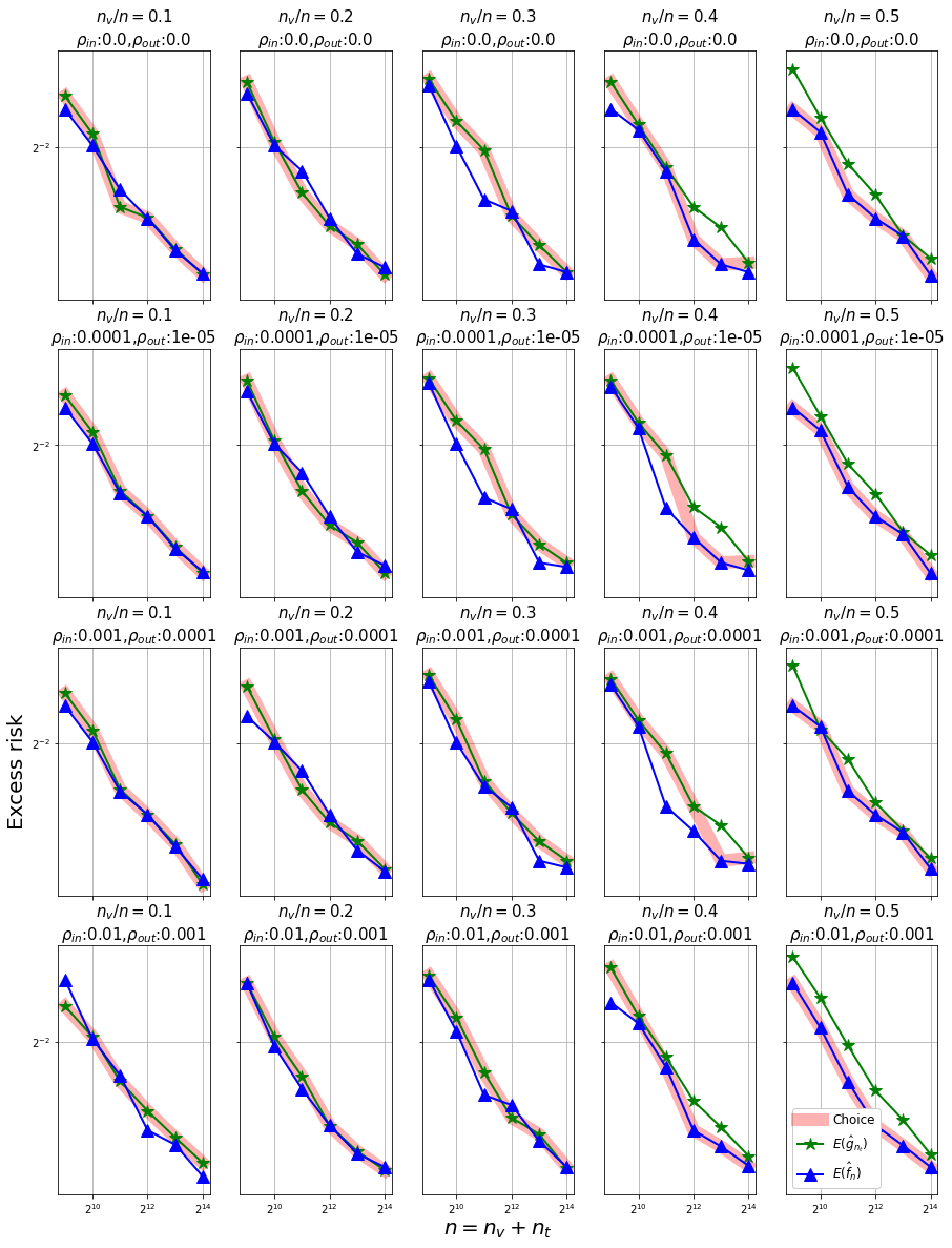
(a) $\rho_{\text{{\footnotesize\tt out}}}=\nicefrac{{\rho_{\text{{\footnotesize\tt in}}}}}{{10}}$

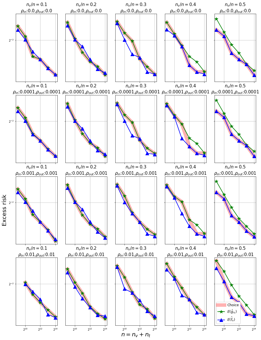
(b) $\rho_{\text{{\footnotesize\tt out}}}=\rho_{\text{{\footnotesize\tt in}}}$

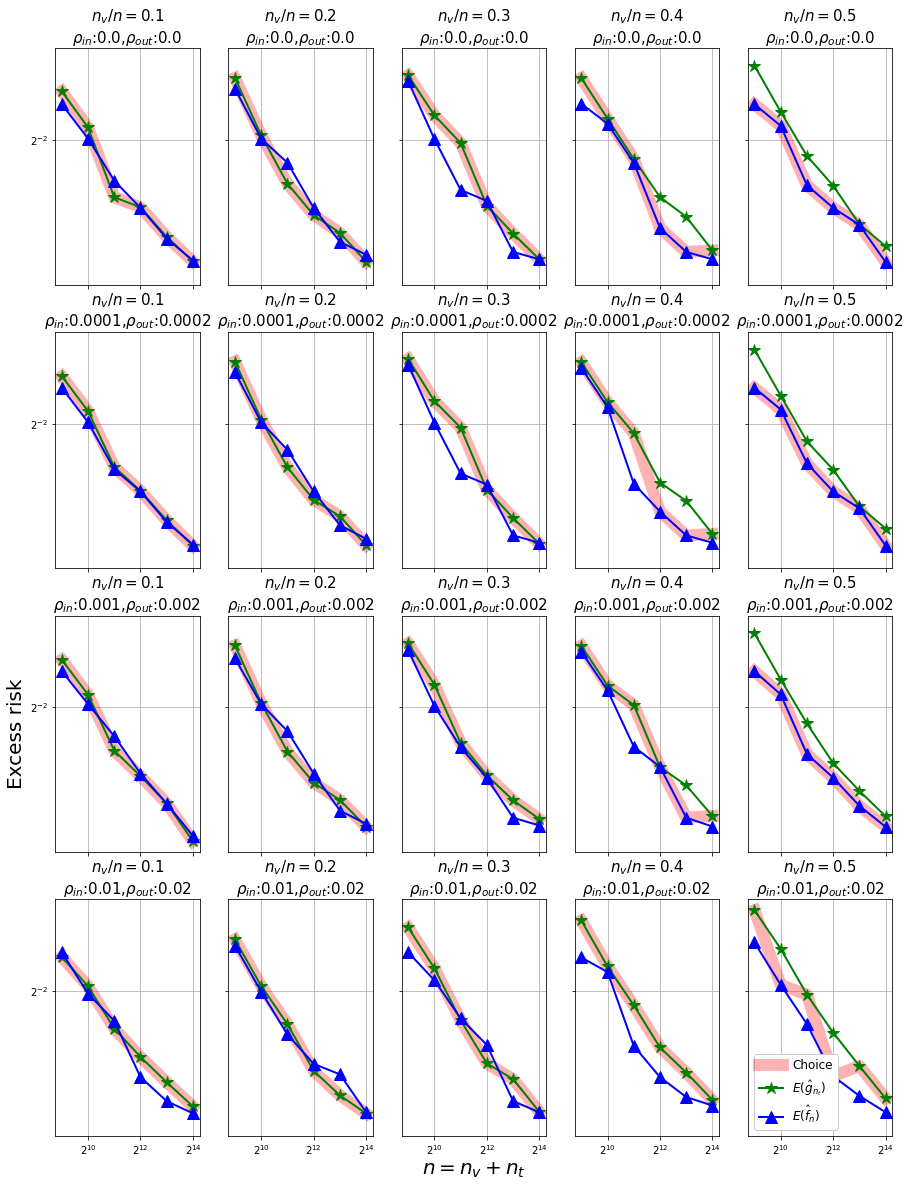
(c) $\rho_{\text{{\footnotesize\tt out}}}=2\cdot\rho_{\text{{\footnotesize\tt in}}}$

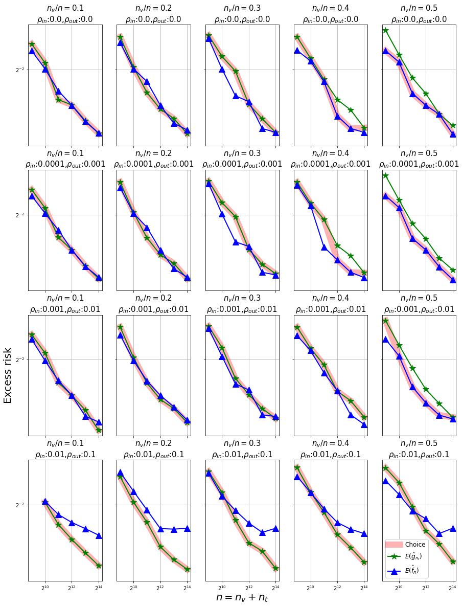
(d) $\rho_{\text{{\footnotesize\tt out}}}=10\cdot\rho_{\text{{\footnotesize\tt in}}}$

Figure 5: Excess-risk of data-dependent choice between $\tilde{f}_{n,\hat{\lambda}}$ and $\tilde{\mathrm{g}}_{n,\hat{\lambda}}$ based on Heuristic 3.1 for $\rho_{\text{{\footnotesize\tt in}}}\in\{0.0001,0.001,0.01,0.1\}$ and search space with $|\Lambda|=18$. Please magnify to view in detail.

D.2 Evaluation of Heuristic B.1

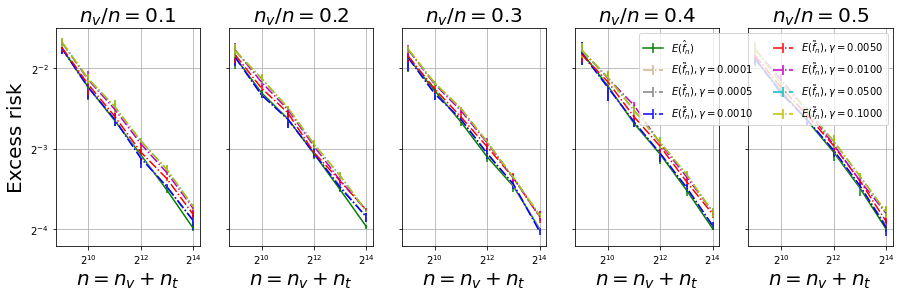
(a) Excess-risk of $\tilde{f}$ vs. $\hat{f}$.

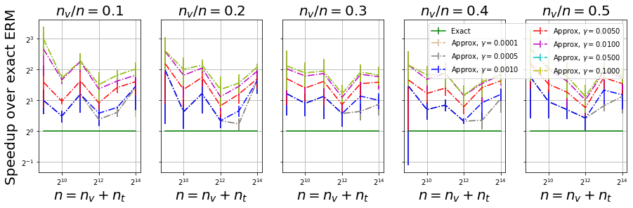
(b) Speedup over exact ERM

Figure 6: Empirical validation of the data-dependent choice of $\rho_{\text{{\footnotesize\tt out}}}$ in Heuristic B.1. Please magnify to view in detail.

Leveraging the data-dependent selection of $\rho_{\text{{\footnotesize\tt out}}}$ with Heuristic B.1, we evaluate the excess risk incurred by approximating the ERM over $\mathcal{F}_{\hat{\lambda}}$ with all $n$ samples to $\rho_{\text{{\footnotesize\tt out}}}$ tolerance. We present the results for the different values of $\gamma$ in Heuristic B.1 from the set $\{0.001,0.005,0.001,0.005,0.01,0.05,0.01\}$ in Figure 6. The excess risks incurred and the speedups gained from using $\tilde{f}_{n,\hat{\lambda}}$ inplace of $\hat{f}_{n,\hat{\lambda}}$ is visualized in Figure 6 – the solid line corresponds to $\hat{f}_{n,\hat{\lambda}}$ while the dash-dotted lines correspond to $\tilde{f}_{n,\hat{\lambda}}$ for different values of $\gamma$. And the results corresponding to the excess risk in Figure 6(a) indicate that, for $\gamma$ up to $0.005$, the increase in excess-risk is quite small. The speedups obtained for the different choices of $\gamma$ and corresponding data-dependent $\rho_{\text{{\footnotesize\tt out}}}$ in Figure 6(b). It can be seen that we can get up to $2\times$ speedup over exact ERM without losing much in terms of the excess risk (see for $\gamma$ up to $0.005$); for larger values of $\gamma$ we can get up to $4\times$ speedup if we are ready to incur some additional excess risk.

References

- Arlot et al. [2010] Sylvain Arlot, Alain Celisse, et al. A survey of cross-validation procedures for model selection. Statistics surveys, 4:40–79, 2010.