Unbiased estimation and asymptotically valid inference in multivariable Mendelian randomization with many weak instrumental variables

Abstract

Mendelian randomization (MR) is a popular epidemiological approach that utilizes genetic variants as instrumental variables (IVs) to infer the causal relationships between exposures and an outcome in the genome-wide association studies (GWAS) era. It is well-known that the inverse-variance weighted (IVW) estimate of causal effect suffers from bias caused by the violation of valid IV conditions, however, the quantitative degree of this bias has not been well characterized and understood. This paper contributes to the theoretical investigation and practical solution of the causal effect estimation in multivariable MR. First, we prove that the bias of IVW estimate is a product of the weak instrument and estimation error biases, where the estimation error bias is caused linearly by measurement error and confounder biases with a trade-off due to the sample overlap among exposure and outcome GWAS cohorts. Second, we demonstrate that our novel multivariable MR approach, MR using Bias-corrected Estimating Equation (MRBEE), can estimate the causal effect unbiasedly in the presence of many weak IVs. Asymptotic behaviors of IVW and MRBEE are investigated under moderate conditions, where MRBEE is shown superior to IVW in terms of unbiasedness and asymptotic validity. Simulations exhibit that only MRBEE can provide a strongly asymptotically unbiased estimate of causal effect in comparison with existing MR methods. Applied to data from the UK Biobank, MRBEE can eliminate weak instrument and estimation error biases and provide valid causal inferences. R package MRBEE and supplementary materials are available online.

Keywords: Causal Inference, Genome-Wide Association Studies, Inverse-Variance Weighting, Mendelian Randomization, Weak Instrumental Variables.

1 Introduction

A genome-wide association study (GWAS) refers to the identification of genetic variants statistically associated with complex traits or diseases across the whole genome using large population cohorts (Visscher et al., 2017). GWAS typically examines associations between single-nucleotide polymorphisms (SNPs) and a trait but can also handle other genetic variants such as insertion and deletions (indels) and structural variations (SVs) (Gresham et al., 2008). The first example of a successful GWAS was the 2005 GWAS which revealed two genetic variants significantly associated with age-related macular degeneration (Klein et al., 2005). To date, over 5,000 human GWAS have investigated approximately 2,000 diseases and traits and have identified more than 400,000 genetic associations (Wijmenga and Zhernakova, 2018). This groundbreaking work has uncovered numerous compelling associations with human complex traits and diseases, shedding light on the disease mechanisms and enhancing clinical care and personalized medicine (Tam et al., 2019).

Mendelian randomization (MR) is an epidemiological method that utilizes genetic variants as instrumental variables (IVs) to infer whether an exposure causally influences an outcome (Burgess and Thompson, 2021). Since the genotypes of individuals are randomly inherited from their parents and generally do not change during their lifetime, genetic variants are considered to be independent of underlying confounders and hence can be used as IVs to eliminate confounding bias. Early MR studies progressed slowly because individual-level data simultaneously including genotypes and phenotypes were rarely available (Ebrahim and Davey Smith, 2008). Recently, many large GWAS have been published and the corresponding summary statistics are available in databases such as the GWAS Catalog (MacArthur et al., 2017) (https://www.ebi.ac.uk/gwas/), dbGaP (https://www.ncbi.nlm.nih.gov/gap/), and UK biobank (UKBB, Sudlow et al. (2015)) (https://www.ukbiobank.ac.uk/). The accuracy of causal effect estimation is improved and valuable insights into the causal relationships between common risk factors and diseases are uncovered by utilizing MR with GWAS summary data (Wang et al., 2022).

The inverse-variance weighted (IVW) method is the most popular approach used to perform MR with GWAS summary data. A causal effect estimate yielded by the IVW method is supposedly unbiased if three so-called valid IV conditions are satisfied: (IV1) the genetic variants are strongly associated with the exposure; (IV2) the genetic variants are associated with the outcome only through the exposure; and (IV3) the genetic variants are independent of confounders (Bowden et al., 2015). The directed acyclic graph (DAG) of valid IV conditions is shown in panel (a) in Figure 1. Due to the complexity of genetic architecture, conditions IV2 and IV3 are often difficult to validate (Zhu, 2020). Meanwhile, it is challenging to quantify the instrument strength and define a universal criterion for concluding that an IV satisfies condition IV1, although the F statistic can be utilized as a rough measure of weak instrument bias (Burgess et al., 2011). Thus, quantifying and eliminating the bias of IVW estimate in MR analysis will lead to valid causal inference and help to understand disease etiology.

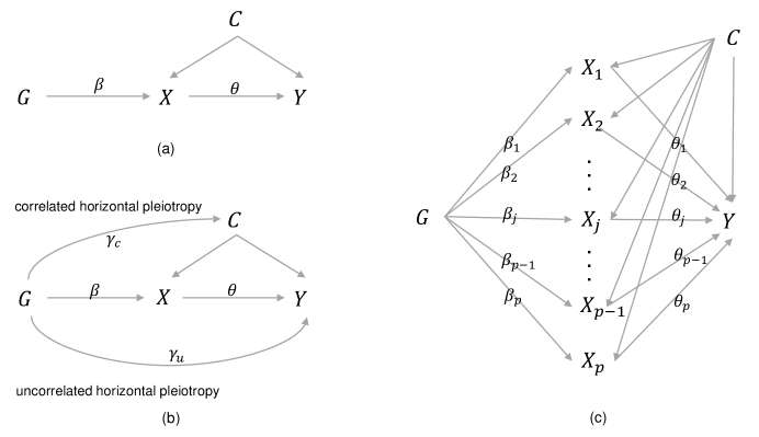
Figure 1: DAG of MR and multivariable MR. Panel (a): causal path digram with valid genetic IVs. Panel (b): causal path digram with UHP and CHP. Panel (c): causal path digram for multivariable MR methods. $G$: genetic IVs; $X$: exposure; $Y$: outcome; $C$: confounders; $\beta$: association between $G$ and $X$; $\theta$: causal effect of $X$ on $Y$; $\gamma_{c}$: direct correlation between $G$ and $C$; $\gamma_{u}$: direct correlation between $G$ and $Y$.

A genetic variant is termed a pleiotropic variant or pleiotropy if it simultaneously affects multiple traits through different pathways. There are two types of pleiotropy: vertical and horizontal pleiotropy, where the former refers to the genetic variant associated with one trait through the mediation of another trait (as described in panel (a) in Figure 1), while the latter refers to the genetic variant independently associated with both traits (as illustrated in panel (b) in Figure 1). IVs with evidence of horizontal pleiotropy should be removed before applying IVW because it violates either the (IV2) condition or the (IV3) condition; otherwise, a biased causal effect estimate is likely obtained. In the literature, there are three strategies to remove the effect of horizontal pleiotropy: 1) Identifying and excluding horizontally pleiotropic IVs by using hypothesis tests, such as the MR pleiotropy residual sum and outlier (MR-PRESSO, Verbanck et al. (2018)) and the iterative MR and pleiotropy (IMRP, Zhu et al. (2021)); 2) Eliminating the effect of horizontal pleiotropy by applying robust tools; e.g., the MR-Egger (Bowden et al., 2015), MR-Median (Bowden et al., 2016), and MR-Lasso/MR-Robust (Rees et al., 2019); 3) Automatically separating vertical pleiotropy from horizontal pleiotropy through a mixture mode, among which the representative methods include MR-Mix (Qi and Chatterjee, 2019) and MR contamination mixture (MR-ConMix, Burgess et al. (2020)).

It has been gradually realized that horizontal pleiotropy can be divided into uncorrelated horizontal pleiotropy (UHP) and correlated horizontal pleiotropy (CHP). UHP violates the (IV2) condition and usually refers to a genetic variant that is directly associated with the outcome. In contrast, CHP violates the IV3 condition and may occur when a genetic variant indirectly affects the outcome through the mediation of unspecified exposures. The DAG of UHP and CHP is shown in panel (b) in Figure 1. Morrison et al. (2020) proposed causal analysis using summary effect (CAUSE), which is the first MR approach accounting for UHP and CHP simultaneously. Cheng et al. (2022) proposed MR-Corr to detect CHP by a Bayesian mixture model and Cheng et al. (2022) extended MR-Corr to MR-CUE (MR with CHP Unraveling shared Etiology and confounding) to detect the UHP and CHP simultaneously. Alternatively, Xue et al. (2021) proposed the constrained maximum likelihood-based MR (cML-MR) method that identifies UHP and CHP through Bayesian information criterion (BIC, Schwarz (1978)). In addition, Yuan et al. (2022) derived MR with automated instrument determination (MRAID) to address UHP and CHP, which allows vertical pleiotropy to be in high linkage disequilibrium (LD).

A significant disadvantage of most existing approaches is that they assume both UHP and CHP to have similar properties as outliers in the traditional regression approach. However, there is substantial evidence that most traits have shared moderate or high genetic correlations (Bulik-Sullivan et al., 2015), violating this technical assumption required by most existing approaches. Consequently, it is challenging to remove the effect of horizontally pleiotropic variants by considering only one exposure in MR analysis. Multivariable MR, which simultaneously estimates the causal effects of multiple exposures on an outcome, is compelling in resolving this problem (Burgess and Thompson, 2015). Multivariable MR recognizes the bias caused by horizontal pleiotropy as an omitted-variable bias (OVB), which will disappear automatically if all the omitted exposures are specified in the multivariable MR model. The DAG of multivariable MR is exhibited in panel (c) in Figure 1. So far, the multivariable versions of the IVW method, MR-Egger, MR-Median, and MR-Lasso/MR-Robust have been developed (Burgess and Thompson, 2015; Rees et al., 2017; Grant and Burgess, 2021). Sanderson et al. (2019) showed that the multivariable MR is able to unbiasedly estimate the causal effects of a target exposure when the other exposure is confounder, collider, or mediator of this exposure.

Weak instrument bias arises when the majority of IVs are weakly associated with the exposures, therefore violating the (IV1) condition and making conventional MR methods unreliable (Burgess et al., 2011). It is widely recognized that a common trait is often polygenic affected by hundreds or even thousands of independent variants/genes with small effect sizes. With the increasing sample sizes of GWAS, more and more trait-associated variants are being identified. Thus, the weak instrument bias is likely to become a considerable problem in future MR studies. Burgess et al. (2011) and Sanderson et al. (2021) suggested using the F and conditional F statistics to measure the weak instrument bias in MR and multivariable MR, respectively. Burgess et al. (2016) illustrated that the weak instrument bias also depends on the sample overlap in two-sample MR. Sadreev et al. (2021) examined the impact of sample overlap and winner’s curse when weak instrument bias exists and observed that the weak instrument bias grew dramatically in the presence of winner’s curse. For the univariate MR model with no sample overlap, Zhao et al. (2020) proposed the robust adjusted profile score to estimate the causal effect unbiasedly, while Ye et al. (2021) provided the debiased IVW (DIVW) method to remove the weak instrument bias of IVW estimate. Overall, these aforementioned methods have neither provided a comprehensive theoretical analysis of weak instrument bias nor a general solution to remove the weak instrument bias in both univariable MR and multivariable MR.

As the first contribution of this paper, we theoretically characterize the bias in multivariable IVW causal estimate. Specifically, we demonstrate that the bias of IVW causal estimate is the product of weak instrument and estimation error biases. Meanwhile, we demonstrate that the estimation error bias is a linear combination of measurement error (Yi, 2017) and confounder biases, and the sample overlaps among multiple GWAS cohorts trade off the proportions of these two biases. With moderate conditions on the MR model, we theoretically illustrate how the number of IVs, sample sizes of GWAS studies, and sample overlap among GWAS cohorts influence the asymptotic behavior of multivariable IVW estimate. These theoretical findings are summarized in Theorem 2 that to our best knowledge is the first comprehensive investigation of multivariable IVW estimate.

As the second contribution of this paper, we demonstrate our novel multivariable MR approach, MR using Bias-corrected Estimating Equations (MRBEE), can estimate causal effects unbiasedly in the presence of many weak IVs. Under moderate conditions, we investigate the asymptotic behaviors of IVW and MRBEE, revealing that MRBEE is superior to IVW in terms of strongly asymptotic unbiasedness. In particular, only when an estimate is strongly asymptotically unbiased, the inference made based on this estimate is asymptotically valid. Simulations show that only MRBEE can provide unbiased causal effect estimates in the presence of many weak IVs. Applied to data from the UK Biobank, MRBEE can successfully remove the weak instrument and estimation error biases and therefore make valid causal inferences.

This paper is arranged as follows. In section 2, we study the asymptotic behavior of multivariate IVW estimate. In section 3, we introduce MRBEE and examine its asymptotic properties. In section 4, simulations are conducted to compare MRBEE with the existing methods. In section 5, we apply MRBEE to estimate the causal effects of exposures on cardiovascular disease. Discussion is presented in section 6 and proofs of the related theorems are shown in Appendix. R package MRBEE (https://github.com/noahlorinczcomi/MRBEE) and supplementary materials are available online.

2 Mendelian Randomization

In this section, we introduce the notations, the model of the multivariable MR, and the bias of the multivariable IVW. Since univariable MR is a special case of multivariable MR, MR refers to the multivariable MR unless otherwise specified.

2.1 Notation

For a vector $\bm{a}=(a_{j})_{p\times 1}$, $||\bm{a}||_{q}=(\sum_{j=1}^{p}|a_{j}|^{q})^{1/q}$ with $q\in[0,\infty]$. For a symmetric matrix $\mathbf{A}=(A_{ij})_{p\times p}$, $\lambda_{\max}(\mathbf{A})$ and $\lambda_{\min}(\mathbf{A})$ is its the maximum and minimum eigenvalues, $\mathbf{A}^{+}$ is its Moore–Penrose inverse; and $||\mathbf{A}||_{q}=\max\{||\mathbf{A}\bm{a}||_{q},\ ||\bm{a}||_{q}=1\}$. Let diag($\bm{\alpha}$) be the diagonalizing operator of vector $\bm{\alpha}$ and $\mathbf{A}\odot\mathbf{B}$ be the Hadamard product of matrices $\mathbf{A}$ and $\mathbf{B}$. For a set $\mathcal{A}$, $|\mathcal{A}|$ is the number of elements in $\mathcal{A}$. Notations $O(\cdot)$ and $o(\cdot)$ are the infinitely large and small quantities, while $O_{P}(\cdot)$ and $o_{P}(\cdot)$ mean that such relationships hold in probability.

2.2 Mendelian randomization model

The central aim of MR is to estimate causal effects between exposures and an outcome unbiasedly. Let $\bm{g}_{i}=(g_{i1},\dots,g_{im})^{\top}$ be an ($m\times 1$) genotype value vector of $m$ genetic variants, $\bm{x}_{i}=(x_{i1},\dots,x_{ip})^{\top}$ be an ($p\times 1$) vector representing $p$ exposures, and $y_{i}$ be an outcome. Here, $m$ is the number of specified IVs, which is usually the number of independent loci with $p$-values reaching the genome-wide significant level. Let $\mathbf{B}=(\bm{\beta}_{1},\dots,\bm{\beta}_{m})^{\top}$ be an ($m\times p$) matrix of genetic effects on exposures with $\bm{\beta}_{j}=(\beta_{j1},\dots,\beta_{jp})^{\top}$ being an $(p\times 1)$ vector, and $\bm{\theta}=(\theta_{1},\dots,\theta_{p})^{\top}$ be an $(p\times 1)$ vector of causal effects of the $p$ exposures on the outcome. The MR model is

$$y_{i} =\bm{x}_{i}^{\top}\bm{\theta}+v_{i},$$ (1)

$$\bm{x}_{i} =\mathbf{B}^{\top}\bm{g}_{i}+\bm{u}_{i}$$ (2)

where $\bm{u}_{i}$ and $v_{i}$ are the noise terms. Substituting for $\bm{x}_{i}$ in (1), we obtain the equation

$$y_{i}=\bm{\alpha}^{\top}\bm{g}_{i}+\bm{\theta}^{\top}\bm{u}_{i}+v_{i},$$ (3)

where $\bm{\alpha}=\mathbf{B}\bm{\theta}$. In the literature, (1) - (3) have been named as the structural form, first-stage, and reduced form, respectively (Stock et al., 2002).

In this paper, we assume that the total number of exposures $p$ is fixed and the causal effect $\bm{\theta}$ is fixed and bounded. The genetic variant $g_{ij}$ is standardized so that E$(g_{ij})=0$ and var$(g_{ij})=1$, and all IVs are in linkage equilibrium (LE), i.e., cov$(g_{ij},g_{ik})=0$ for $j\neq k$. The genetic effect $\bm{\beta}_{j}$ is random with zero-mean, covariance matrix $\bm{\Sigma}_{\beta\beta}$, and cumulative covariance matrix $\bm{\Psi}_{\beta\beta}$

$$\bm{\Sigma}_{\beta\beta}=\text{E}(\bm{\beta}_{j}\bm{\beta}_{j}^{\top}),\quad\bm{\Psi}_{\beta\beta}=m\bm{\Sigma}_{\beta\beta}.$$

The covariance matrix $\bm{\Sigma}_{\beta\beta}$ will vanish as $m$ increase, but the cumulative covariance matrix $\bm{\Psi}_{\beta\beta}$ is still a constant matrix, representing the total genetic covariance contributed from the $m$ IVs. Next, the noise terms $\bm{u}_{i}$ and $v_{j}$ have zero-means and joint covariance matrix

$$\bm{\Sigma}_{u\times v}=\text{cov}((\bm{u}_{i}^{\top},v_{j})^{\top})=\begin{pmatrix}\bm{\Sigma}_{uu}&\bm{\sigma}_{uv}\\ \bm{\sigma}_{uv}^{\top}&\sigma_{vv}.\end{pmatrix}$$

Thus, the exposure vector $\bm{x}_{i}$ and outcome $y_{i}$ have zero-means and joint covariance matrix

$$\bm{\Sigma}_{x\times y}=\text{cov}((\bm{x}_{i}^{\top},y_{j})^{\top})=\begin{pmatrix}\bm{\Sigma}_{xx}&\bm{\sigma}_{xy}\\ \bm{\sigma}_{xy}^{\top}&\sigma_{yy}.\end{pmatrix}$$

where $\mathbf{\Sigma}_{xx}=\bm{\Psi}_{\beta\beta}+\bm{\Sigma}_{uu}$, $\bm{\sigma}_{xy}=\bm{\Psi}_{\beta\beta}\bm{\theta}+\mathbf{\Sigma}_{uu}\bm{\theta}+\bm{\sigma}_{uv}$, and $\sigma_{yy}=\bm{\theta}^{\top}\bm{\Psi}_{\beta\beta}\bm{\theta}+\bm{\theta}^{\top}\bm{\Sigma}_{uu}\bm{\theta}+2\bm{\theta}^{\top}\bm{\sigma}_{uv}+\sigma_{vv}.$ Note that $\bm{\sigma}_{uv}\neq\mathbf{0}$ means the confounders simultaneously affect $\bm{x}_{i}$ and $y_{i}$.

In genetics, the genetic effect $\beta_{js}$ can be treated as a random variable with mean 0 and variance $\psi_{\beta_{s}\beta_{s}}/m$, where $\psi_{\beta_{s}\beta_{s}}$ is the IV-heritability, i.e., the variance explained by additive effects of specified instrumental variants of the $s$th exposure (Bulik-Sullivan et al., 2015). Since a complex trait is often polygenic with a contribution from thousands of independent variants, the number of causal variants can be regarded as a number approaching infinity. Subject to this principle, a random effect model can describe the variation of these effects more simply and essentially. Although the fixed effect model has also been adopted by some works to study the asymptotic properties of the corresponding MR approaches (Zhao et al., 2020; Ye et al., 2021), the random effect model is still the most commonly used at genome-wide level studies. Moreover, even if all causal variants were identified, the random effect model should still be more efficient than the fixed effect model to characterize the statistical property of the MR model (Diggle et al., 2002).

The existing univariable MR methods, such as CAUSE (Morrison et al., 2020) and MR-CUE (Cheng et al., 2022), can successfully remove the effects of CHP only when a small fraction of IVs have CHP, which is easy to violate because common traits may share a large fraction of pleiotropic variants (Bulik-Sullivan et al., 2015). In contrast, multivariable MR resolves the pleiotropic variant problem by specifying all the relevant exposures in the model (1), as the multivariable regression can automatically account for the pleiotropic variants shared by these exposures. This is one of the greatest advantages of multivariable MR over univariable MR. Hence, we assume that all the exposures can be included in the multivariable MR; therefore, the CHP effect is ignorable in (1). On the other hand, some IVs may still present strong UHP effects. To account for potential UHP, we propose using an iterative procedure to remove these invalid IVs, which is similar to detecting outliers in MR analysis (Verbanck et al., 2018; Zhu, 2020). Thus, the bias introduced by UHP and CHP can be greatly alleviated, as demonstrated in our proposed MRBEE.

2.3 Mendelian randomization with GWAS summary data

With the rapid development of GWAS, large GWASs of exposures and disease outcomes have been conducted and their summary statistics including effect sizes, SEs, and variant information are publicly available for download (Sudlow et al., 2015; MacArthur et al., 2017). Thus, many recently developed MR methods are often designed based on GWAS summary statistics, as is in this paper.

With GWAS summary statistics, MR is mainly based on the linear regression model

$$\hat{\alpha}_{j}=\hat{\bm{\beta}}_{j}^{\top}\bm{\theta}+\varepsilon_{j},$$ (4)

where $\hat{\alpha}_{j}$ and $\hat{\bm{\beta}}_{j}$ are estimated from outcome and exposure GWAS for $j$th IV, and $\varepsilon_{j}$ represents the residual of this regression model. Let $\mathbf{y}^{[0]}=(y^{[0]}_{1},\dots,y^{[0]}_{n_{0}})^{\top}$ be the sample vector from outcome GWAS, $\bm{x}^{[1]}=(x^{[1]}_{1},\dots,x^{[1]}_{n_{1}})^{\top},\dots,\bm{x}^{[p]}=(x^{[p]}_{1},\dots,x^{[p]}_{n_{p}})^{\top}$ be the sample vectors of the 1st$,\dots,p$th exposure GWAS cohorts, and $\mathbf{G}^{[0]}=(g^{[0]}_{ij})_{n_{0}\times m},\dots,\mathbf{G}^{[p]}=(g^{[p]}_{ij})_{n_{p}\times m}$ be the sample matrices of $m$ genetic variants of the outcome and 1st$,\dots,p$th exposure GWAS cohorts. The sample size of the $s$th cohort is $n_{s}$, the overlapping sample size between the $s$th and the $k$th cohorts is $n_{sk}$, and the minimum sample size is $n_{\rm min}=\min\{n_{0},\dots,n_{p}\}$.

The GWAS summary data are generated as follows. Suppose that $\bm{y}^{[0]}$, $\{\bm{x}^{[s]}\}$, and $\{\mathbf{G}^{[s]}\}$ are centered, and the $m$ genetic variants are in LE, i.e. ${\rm E}(\mathbf{G}^{[s]\top}\mathbf{G}^{[s]}/n_{s})=\mathbf{I}_{m}$ for $j=0,1,\dots,p$. This orthogonality enables the following genetic effects to be estimated separately

$$\hat{\alpha}_{j}=\frac{\bm{g}_{j}^{[0]\top}\bm{y}^{[0]}}{n_{0}},\quad\hat{\beta}_{js}=\frac{\bm{g}_{j}^{[s]\top}\bm{x}^{[s]}}{n_{s}},$$ (5)

where the corresponding variance estimates are given by

$$\text{var}(\hat{\alpha}_{j})=\frac{\sigma_{yy}-\bm{\theta}^{\top}\bm{\Sigma}_{\beta\beta}\bm{\theta}}{n_{0}}\approx\frac{\sigma_{yy}}{n_{0}},\quad\text{var}(\hat{\beta}_{js})=\frac{\sigma_{x_{s}x_{s}}-\sigma_{\beta_{s}\beta_{s}}}{n_{s}}\approx\frac{\sigma_{x_{s}x_{s}}}{n_{s}}.$$ (6)

Then the GWAS summary data are formed by $\hat{\bm{\alpha}}=(\hat{\alpha}_{1},\dots,\hat{\alpha}_{m})^{\top}$, $\hat{\bm{\beta}}_{j}=(\hat{\beta}_{j1},\dots,\hat{\beta}_{jp})^{\top}$, $\hat{\mathbf{B}}=(\hat{\bm{\beta}}_{1},\dots,\hat{\bm{\beta}}_{m})^{\top}$, the related SE estimates, the p-values, and sample sizes $n_{0},n_{1},\dots,n_{p}$, and SNPs information.

The IVW method is equivalent to a weighted regression which estimates $\bm{\theta}$ by

$$\hat{\bm{\theta}}_{\rm IVW}=\arg\min_{\bm{\theta}}\bigg{\{}\frac{1}{2m}\sum_{j=1}^{m}\frac{(\hat{\alpha}_{j}-\hat{\bm{\beta}}_{j}^{\top}\bm{\theta})^{2}}{{\text{var}}(\hat{\alpha}_{j})}\bigg{\}}=(\hat{\mathbf{B}}^{\top}\mathbf{V}\hat{\mathbf{B}})^{-1}\hat{\mathbf{B}}^{\top}\mathbf{V}\hat{\bm{\alpha}},$$ (7)

where $\mathbf{V}=\text{diag}(1/\text{var}(\hat{\alpha}_{1}),\dots,1/\text{var}(\hat{\alpha}_{m}))$. In practice, we often standardize $\hat{\alpha}_{j}$ and $\hat{\beta}_{js}$ by $\hat{\alpha}_{j}/\text{se}(\hat{\alpha}_{j})$ and $\hat{\beta}_{js}/\text{se}(\hat{\beta}_{js})$ to remove the minor allele frequency effect (Zhu et al., 2022). Therefore, ${\text{var}}(\hat{\alpha}_{j})=1$ for all $j$ and (7) reduces to

$$\hat{\bm{\theta}}_{\rm IVW}=\arg\min_{\bm{\theta}}\bigg{\{}\frac{1}{2m}\|\hat{\bm{\alpha}}-\hat{\mathbf{B}}\bm{\theta}\|_{\text{2}}^{2}\bigg{\}}=(\hat{\mathbf{B}}^{\top}\hat{\mathbf{B}})^{-1}\hat{\mathbf{B}}^{\top}\hat{\bm{\alpha}}.$$ (8)

Here, we qualitatively show that the IVW estimate is biased due to the estimation errors of $\hat{\bm{\alpha}}$ and $\hat{\mathbf{B}}$, i.e., ${\bm{w}}_{\alpha}=\hat{\bm{\alpha}}-\bm{\alpha}$ and ${\mathbf{W}}_{\beta}=\hat{\mathbf{B}}-\mathbf{B}$, and meanwhile, the weak IVs can inflate th estimation error bias. Specifically, consider the estimating equation and Hessian matrix of $\hat{\bm{\theta}}_{\rm IVW}$:

$$\bm{S}_{\rm IVW}(\bm{\theta})=-\frac{\hat{\mathbf{B}}^{\top}(\hat{\bm{\alpha}}-\hat{\mathbf{B}}\bm{\theta})}{m}= \frac{1}{m}\bigg{(}-\mathbf{B}^{\top}\bm{w}_{\alpha}-\mathbf{B}^{\top}\mathbf{W}_{\beta}\bm{\theta}+\mathbf{W}_{\beta}^{\top}\bm{w}_{\alpha}-\mathbf{W}_{\beta}^{\top}\mathbf{W}_{\beta}\bm{\theta}\bigg{)},$$ (9)

$$\textbf{H}_{\rm IVW}=\frac{\hat{\mathbf{B}}^{\top}\hat{\mathbf{B}}}{m}= \frac{1}{m}\bigg{(}\mathbf{B}^{\top}\mathbf{B}+\mathbf{W}_{\beta}^{\top}\mathbf{W}_{\beta}+\mathbf{B}^{\top}\mathbf{W}_{\beta}+\mathbf{W}_{\beta}^{\top}\mathbf{B}\bigg{)}.$$ (10)

That is, $\bm{S}_{\rm IVW}(\bm{\theta})$ is the score function of (8) and $\hat{\bm{\theta}}_{\rm IVW}$ is estimated by solving $\bm{S}_{\rm IVW}(\hat{\bm{\theta}}_{\rm IVW})=\mathbf{0}$, and $\textbf{H}_{\rm IVW}$ is the second order derivative matrix of (8). In particular, since the third derivative of the quadratic loss function (8) is zero, we have $\hat{\bm{\theta}}_{\rm IVW}-\bm{\theta}=-\textbf{H}_{\rm IVW}^{-1}\bm{S}_{\rm IVW}(\bm{\theta})$. As a result, the expectation of the bias of $\hat{\bm{\theta}}_{\rm IVW}$ is approximately:

$${\rm E}(\hat{\bm{\theta}}_{\rm IVW}-\bm{\theta}) \approx-{\rm E}(\textbf{H}_{\rm IVW})^{-1}{\rm E}(\bm{S}_{\rm IVW}(\bm{\theta}))$$

$$=-\underbrace{\bigg{\{}\mathbf{\Sigma}_{\beta\beta}+\bm{\Sigma}_{W_{\beta}W_{\beta}}\bigg{\}}^{-1}}_{\text{weak instrument bias}}\underbrace{\bigg{\{}\bm{\Sigma}_{W_{\beta}W_{\beta}}\bm{\theta}-\bm{\sigma}_{W_{\beta}w_{\alpha}}\bigg{\}}}_{\text{estimation error bias}},$$ (11)

where ${\bm{w}}_{\beta_{j}}$ is the $j$th row of ${\mathbf{W}}_{\beta}$, $w_{\alpha_{j}}$ is the $j$th element of ${\bm{w}}_{\alpha}$, and

$$\text{cov}(({\bm{w}}_{\beta_{j}}^{\top},w_{\alpha_{j}})^{\top})=\bm{\Sigma}_{W_{\beta}\times w_{\alpha}}=\begin{pmatrix}\bm{\Sigma}_{W_{\beta}W_{\beta}}&\bm{\sigma}_{W_{\beta}w_{\alpha}}\\ \bm{\sigma}_{W_{\beta}w_{\alpha}}^{\top}&\sigma_{w_{\alpha}w_{\alpha}}.\end{pmatrix},$$

Intuitively, the bias of $\hat{\bm{\theta}}_{\rm IVW}$ has a product structure “weak instrument bias $\times$ estimation error bias”. We call $\{\bm{\Sigma}_{W_{\beta}W_{\beta}}\bm{\theta}-\bm{\sigma}_{W_{\beta}w_{\alpha}}\}$ the estimation error bias because it comes from the covariance matrix of estimation errors $\bm{\Sigma}_{W_{\beta}\times w_{\alpha}}$. We term $\{\mathbf{\Sigma}_{\beta\beta}+\bm{\Sigma}_{W_{\beta}W_{\beta}}\}$ the weak instrument bias because the bias of $\hat{\bm{\theta}}_{\rm IVW}$ is inflated if the covariance matrix of effect sizes $\mathbf{\Sigma}_{\beta\beta}$ is not considerably larger than the covariance matrix of estimation errors $\bm{\Sigma}_{W_{\beta}W_{\beta}}$, which often happens if the majority of IVs used to infer the causal effect have weak effects.

2.4 Asymptotic behavior of IVW estimate

In this subsection, we investigate the asymptotic behavior of the IVW estimate as the number of IVs $m$ and the minimum sample size $n_{\min}$ go to infinity. To facilitate the theoretical derivation, we specify the following three definitions and four regularity conditions.

Definition 1 (Sub-Gaussian variable).

A random variable $x$ is sub-Gaussian distributed with sub-Gaussian parameter $\tau_{x}>0$ if for all $t>0$, $\Pr(|x-E(x)|\geq t)\leq 2e^{-t^{2}/\tau_{x}^{2}}$.

Definition 2 (Well-conditioned covariance matrix).

A covariance matrix $\bm{\Sigma}$ is well-conditioned if there is a positive constant $d_{0}$ such that $0<d_{0}^{-1}\leq\lambda_{\min}(\bm{\Sigma})\leq\lambda_{\max}(\bm{\Sigma})\leq d_{0}<\infty.$

Definition 3 (Strongly asymptotically unbiased estimate).

Let $\hat{\bm{\theta}}$ be a consistent estimate of $\bm{\theta}$ with an asymptotic normal distribution $\sqrt{s}_{n}(\hat{\bm{\theta}}-\bm{\theta})\stackrel{{\scriptstyle D}}{{\longrightarrow}}\mathcal{N}(\bm{\mu}_{\theta},\bm{\Sigma}_{\theta})$, where $\bm{\mu}_{\theta}$ is a vector with a bounded $\ell_{2}$-norm, $\bm{\Sigma}_{\theta}$ is a well-conditioned covariance matrix, and $s_{n}$ is a sequence of $n$. Then $\hat{\bm{\theta}}$ is called a strongly asymptotically unbiased estimate of $\bm{\theta}$ if $\bm{\mu}_{\theta}=\mathbf{0}$.

A sub-Gaussian variable is one of the basic concepts in modern statistics (Vershynin, 2018). It generalizes the scope of ordinary Gaussian variables to include all bounded discrete and common continuous variables. The well-conditioned covariance matrix is another important concept (Bickel and Levina, 2008). A well-conditioned covariance matrix will ensure that the related statistical optimization is nondegenerate. In addition, we define the strongly asymptotic unbiasedness to distinguish the consistent estimate whose bias square vanishes with an equal and a smaller rate than its variance, respectively. If an estimate is consistent but its bias square and variance vanish at the same rate, the classic confidence interval cannot cover the true parameter with a probability of 0.95, thus leading to invalid statistical inference. This problem widely exists in all fields of statistics, especially, in nonparametric statistics and high-dimensional statistics, and many novel methods are derived to reduce the bias such that the bias square vanishes faster than the variance (Hall, 1992; Van de Geer et al., 2014; Jankova and Van De Geer, 2018; Calonico et al., 2018).

Condition 1 (Regularity conditions for multivariable MR).

• For $\bm{g}_{i}=(g_{i1},\dots,g_{im})^{\top}$, each entry $g_{ij}$ is a bounded sub-Gaussian variable with E$(g_{ij})=0$, var($g_{ij}$)=1, and sub-Gaussian parameter $\tau_{g}\in(0,\infty)$. For all $(i,j)\neq(t,s)$, $g_{ij}$ is independent of $g_{ts}$.

• For $\bm{u}_{i}=(u_{i1},\dots,u_{ip})^{\top}$, each entry $u_{ij}$ is a sub-Gaussian variable with E$(u_{ij})=0$, var($u_{is})\in(0,\infty)$, and sub-Gaussian parameter $\tau_{u}\in(0,\infty)$; $v_{i}$ is a sub-Gaussian variable with E$(v_{i})=0$, var($v_{i})\in(0,\infty)$, and sub-Gaussian parameter $\tau_{v}\in(0,\infty)$. Besides, $(\bm{u}_{i}^{\top},v_{i})^{\top}$ is independent of $(\bm{u}_{t}^{\top},v_{t})^{\top}$ for all $i\neq t$. Furthermore, $\mathbf{\Sigma}_{u\times v}$ is a well-conditioned covariance matrix of $(\bm{u}_{i}^{\top},v_{i})^{\top}$.

• For $\bm{\beta}_{j}=(\beta_{j1},\dots,\beta_{jp})^{\top}$, $\sqrt{m}\beta_{js}$ is a sub-Gaussian variable with E$(\sqrt{m}\beta_{js})=0$, var($\sqrt{m}\beta_{js})\in(0,\infty)$, and sub-Gaussian parameter $\tau_{\beta}\in(0,\infty)$. For all $j\neq t$, $\bm{\beta}_{j}$ is independent of $\bm{\beta}_{t}$. In addition, $\bm{\Psi}_{\beta\beta}$ is a well-conditioned covariance matrix of $\sqrt{m}\bm{\beta}_{j}$.

• The genetic variant $g_{ij}$, the genetic effect $\bm{\beta}_{j}$, the noise terms $\bm{u}_{i}$ and $v_{i}$, are three mutually independent groups.

Conditions (C1)-(C4) restrict that all variables involved in this paper are sub-Gaussian distributed. In practice, $g_{ij}$ is standardized from a binomial variable with status 0, 1, and 2. Hence, it is supposedly a bounded sub-Gaussian variable as long as its minor allele frequency is not rare. Besides, we assume $\sqrt{m}\bm{\beta}_{j}$ to be sub-Gaussian with a well-conditioned covariance matrix $\bm{\Psi}_{\beta\beta}$ because the covariance explained by each variant $\bm{\Sigma}_{\beta\beta}$ decreases as the number of instrumental variants $m$ increases.

Theorem 1.

Denote $w_{\alpha_{j}}=\hat{\alpha}_{j}-\alpha_{j}$ and $\omega_{js}=\hat{\beta}_{js}-\beta_{js}$, $s=1,\dots,p$. Then for all $j$,

$$\begin{pmatrix}\sqrt{n}_{0}w_{\alpha_{j}}\\ \sqrt{n}_{1}w_{\beta_{1j}}\\ \vdots\\ \sqrt{n}_{p}w_{\beta_{1p}}\end{pmatrix}\stackrel{{\scriptstyle D}}{{\longrightarrow}}\mathcal{N}\begin{pmatrix}\begin{pmatrix}0\\ 0\\ \vdots\\ 0\end{pmatrix},\begin{pmatrix}\sigma_{yy}&\frac{n_{01}}{\sqrt{n_{0}n_{1}}}\sigma_{yx_{1}}&\cdots&\frac{n_{01}}{\sqrt{n_{0}n_{p}}}\sigma_{yx_{p}}\\ \frac{n_{01}}{\sqrt{n_{0}n_{1}}}\sigma_{yx_{1}}&\sigma_{x_{1}x_{1}}&\cdots&\frac{n_{1p}}{\sqrt{n_{1}n_{p}}}\sigma_{x_{1}x_{p}}\\ \vdots&\vdots&\ddots&\vdots\\ \frac{n_{0p}}{\sqrt{n_{0}n_{p}}}\sigma_{yx_{p}}&\frac{n_{1p}}{\sqrt{n_{1}n_{p}}}\sigma_{x_{1}x_{p}}&\cdots&\sigma_{x_{p}x_{p}}\end{pmatrix}\end{pmatrix},$$

if $n_{0},\dots,n_{p}$ and $m\to\infty$.

Theorem 1 demonstrates the asymptotic normal distribution of the estimation errors, based on which we are able to obtain

$$\bm{\Sigma}_{W_{\beta}W_{\beta}}=\mathbf{\Delta}_{xx}\odot\bm{\Sigma}_{xx},\quad\bm{\sigma}_{W_{\beta}w_{\alpha}}=\bm{\delta}_{xy}\odot\bm{\sigma}_{xy},\quad\sigma_{w_{\alpha}w_{\alpha}}=\sigma_{yy}/n_{0},$$ (12)

where the $(j,s)$th element of $\mathbf{\Delta}_{xx}$ is $n_{js}/(n_{j}n_{s})$ and the $j$th element of $\bm{\delta}_{xy}$ is $n_{j0}/(n_{0}n_{j})$. As a result, the expectations of $\bm{S}_{\rm IVW}(\bm{\theta})$ and $\mathbf{H}_{\rm IVW}$ are given by

$${\rm E}(\bm{S}_{\rm IVW}(\bm{\theta})) =(\mathbf{\Delta}_{xx}\odot\bm{\Sigma}_{xx})\bm{\theta}-\bm{\delta}_{xy}\odot\bm{\sigma}_{xy},$$ (13)

$${\rm E}(\mathbf{H}_{\rm IVW}) =\mathbf{\Sigma}_{\beta\beta}+\mathbf{\Delta}_{xx}\odot\bm{\Sigma}_{xx}.$$ (14)

By expressing $\bm{\sigma}_{xy}=\mathbf{\Sigma}_{xx}\bm{\theta}+\bm{\sigma}_{uv}$, we obtain an alternative expectation of $\bm{S}_{\rm IVW}(\bm{\theta}))$:

$$\underbrace{\text{E}(\bm{S}_{\rm IVW}(\bm{\theta}))}_{\text{estimation bias}}=\underbrace{\{(\mathbf{\Delta}_{xx}-\bm{\delta}_{xy}\mathbf{1}^{\top})\odot\bm{\Sigma}_{xx}\}\bm{\theta}}_{\text{measurement error bias}}-\underbrace{\bm{\delta}_{xy}\odot\bm{\sigma}_{uv}}_{\text{confounder bias}}.$$ (15)

From this expectation, it is clear that there are two sources of the estimation error bias: $\{(\mathbf{\Delta}_{xx}-\bm{\delta}_{xy}\mathbf{1}^{\top})\odot\bm{\Sigma}_{xx}\}\bm{\theta}$ comes from the measurement error, while $\{\bm{\delta}_{xy}\odot\bm{\sigma}_{uv}\}$ is caused by the confounder. Here, we call $\{(\mathbf{\Delta}_{xx}-\bm{\delta}_{xy}\mathbf{1}^{\top})\odot\bm{\Sigma}_{xx}\}\bm{\theta}$ the measurement error bias because it has the same statistical impact, i.e., shrinking the coefficient estimate toward zero, as in measurement error analysis (Yi, 2017). In contrast, we term $\{\bm{\delta}_{xy}\odot\bm{\sigma}_{uv}\}$ the confounder bias because $\bm{\sigma}_{uv}\neq\mathbf{0}$ implies that there are underlying confounders simultaneously affecting both $\bm{x}_{i}$ and $y_{i}$. In addition, the overlapping fraction vector $\bm{\delta}_{xy}$ trades off these two sources of biases. Generally, the measurement error bias is dominant when the elements of $\bm{\delta}_{xy}$ are small, while the confounder bias dominates when the elements of $\bm{\delta}_{xy}$ are large, and there may exist a special sample overlap such that $\bm{\delta}_{xy}\odot\bm{\sigma}_{uv}=\{(\mathbf{\Delta}_{xx}-\bm{\delta}_{xy}\mathbf{1}^{\top})\odot\bm{\Sigma}_{xx}\}\bm{\theta}$. In univariable MR, this special fraction is $n_{01}/n_{0}=\sigma_{xx}\theta/\sigma_{xy}$, which guarantees that E$(S_{\rm IVW}(\theta))=0$ and E$(\hat{\theta}_{\rm IVW})=\theta$. This theoretical result explains why in the empirical studies (e.g., Figures 1 and 2 in Sadreev et al. (2021)), $\hat{\theta}_{\rm IVW}$ has a negative bias when $n_{01}/n_{0}$ is small, positive bias when $n_{01}/n_{0}$ is large, and is unbiased at this specific point.

Theorem 2.

Suppose conditions (C1)-(C4) hold and $m$, $n_{\rm min}\to\infty$. Then

1. if $m/\sqrt{n}_{\min}\to 0$, $\sqrt{n}_{\min}(\hat{\bm{\theta}}_{\rm IVW}-\bm{\theta})\stackrel{{\scriptstyle D}}{{\longrightarrow}}\mathcal{N}(\mathbf{0},\psi_{\theta}\bm{\Psi}_{\beta\beta}^{-1});$

2. if $m/\sqrt{n}_{\min}\to c_{0}$, $\sqrt{n}_{\min}(\hat{\bm{\theta}}_{\rm IVW}-\bm{\theta})\stackrel{{\scriptstyle D}}{{\longrightarrow}}\mathcal{N}(-c_{0}\bm{\Psi}_{\beta\beta}^{-1}(\bm{\Psi}_{W_{\beta}W_{\beta}}\bm{\theta}-\bm{\psi}_{W_{\beta}w_{\alpha}}),\psi_{\theta}\bm{\Psi}_{\beta\beta}^{-1});$

3. if $m/n_{\min}\to c_{0}$, $\hat{\bm{\theta}}_{\rm IVW}-\bm{\theta}\stackrel{{\scriptstyle P}}{{\longrightarrow}}-c_{0}(\bm{\Psi}_{\beta\beta}+c_{0}\bm{\Psi}_{W_{\beta}W_{\beta}})^{-1}(\bm{\Psi}_{W_{\beta}W_{\beta}}\bm{\theta}-\bm{\psi}_{W_{\beta}w_{\alpha}});$

4. if $m/n_{\rm min}\to\infty$, $\hat{\bm{\theta}}_{\rm IVW}\stackrel{{\scriptstyle P}}{{\longrightarrow}}\bm{\Psi}_{W_{\beta}W_{\beta}}^{+}\bm{\psi}_{W_{\beta}w_{\alpha}};$

where

$$\mathbf{\Psi}_{W_{\beta}\times w_{\alpha}}=\begin{pmatrix}\mathbf{\Psi}_{W_{\beta}W_{\beta}}&\bm{\psi}_{W_{\beta}w_{\alpha}}\\ \bm{\psi}_{W_{\beta}w_{\alpha}}^{\top}&\psi_{w_{\alpha}w_{\alpha}}\end{pmatrix}=\lim_{n_{\min}\to\infty}\begin{pmatrix}n_{\min}\bm{\Sigma}_{W_{\beta}W_{\beta}}&n_{\min}\bm{\sigma}_{W_{\beta}w_{\alpha}}\\ n_{\min}\bm{\sigma}_{W_{\beta}w_{\alpha}}^{\top}&n_{\min}\sigma_{w_{\alpha}w_{\alpha}}\end{pmatrix},$$

$\psi_{\theta}=\psi_{w_{\alpha}w_{\alpha}}+\bm{\theta}^{\top}\bm{\Psi}_{W_{\beta}W_{\beta}}\bm{\theta}-2\bm{\theta}^{\top}\bm{\psi}_{W_{\beta}w_{\alpha}}$, and $c_{0}$ is a positive constant.

Theorem 2 is one of two main theorems in this paper and points out four scenarios. First, if $m$ goes to infinity with a lower rate than $\sqrt{n}_{\rm min}$, $\hat{\bm{\theta}}_{\rm IVW}$ is strongly asymptotically unbiased. In other words, $\hat{\bm{\theta}}_{\rm IVW}$ is able to reliably infer causality only when the sample size of GWAS data is quadratically larger than the number of IVs. On the other hand, the asymptotic covariance matrix of $\hat{\bm{\theta}}_{\rm IVW}$ is the inverse of the cumulative covariance matrix $\mathbf{\Psi}_{\beta\beta}=\sum_{j=1}^{m}\text{cov}(\bm{\beta}_{j})$, therefore, it is optimal to include as many associated variants as possible in order to have $\mathbf{\Psi}_{\beta\beta}$ large enough. In contrast, using a few top significant variants to perform MR analysis is not recommended.

Second, if $m$ tends to infinity with the same rate as $\sqrt{n}_{\rm min}$, $\sqrt{n}_{\min}(\hat{\bm{\theta}}_{\rm IVW}-\bm{\theta})$ converges to an asymptotic normal distribution with a non-zero asymptotic bias $\{-c_{0}\bm{\Psi}_{\beta\beta}^{-1}(\bm{\Psi}_{W_{\beta}W_{\beta}}\bm{\theta}-\bm{\psi}_{W_{\beta}w_{\alpha}})\}$. In this asymptotic bias, $\{-c_{0}(\bm{\Psi}_{W_{\beta}W_{\beta}}\bm{\theta}-\bm{\psi}_{W_{\beta}w_{\alpha}})\}$ is caused by $\bm{S}_{\rm IVW}(\bm{\theta})$ and $\bm{\Psi}_{\beta\beta}^{-1}$ is resulted by $\mathbf{H}_{\rm IVW}^{-1}$. Since the asymptotic bias and asymptotic covariance matrix are of the same order in this scenario, the inference made is invalid although the bias of $\hat{\bm{\theta}}_{\rm IVW}$ is infinitesimal. Scenario $(iii)$ is more serious than $(ii)$ because the bias of $\hat{\bm{\theta}}_{\rm IVW}$ will not vanish even when $\sqrt{n}_{\rm min}$ goes to infinity. In the fourth scenario, $\hat{\bm{\theta}}_{\rm IVW}$ converges to a term irrelevant to $\bm{\theta}$. Scenarios (ii) - (iv) indicate that the IVW method is unlikely to make valid causal inference unless the sample sizes are quadratically larger than the number of IVs.

It is crucial to understand the asymptotic behaviors of $\hat{\bm{\theta}}_{\rm IVW}$ since the IVW method serves as the foundation for practically all MR techniques. Specifically, IMRP and MR-PRESSO use hypothesis tests to identify invalid IVs and then apply the IVW method to estimate causal effects based on valid IVs only. MR-Robust and MR-Median replace the quadratic loss function used in IVW by a robust loss function and absolute loss function, respectively. Although there have been literature studying the bias of $\hat{\bm{\theta}}_{\rm IVW}$ empirically (Burgess et al., 2011, 2016), they could not explain what causes the bias and how it behaves asymptotically. In contrast, Theorem 2 points out the asymptotic properties of $\hat{\bm{\theta}}_{\rm IVW}$, representing a significant advance in understanding the IVW method and its extensions.

3 Bias-corrected Estimating Equation

According to (11), it is possible to remove the bias of $\bm{S}_{\rm IVW}(\bm{\theta})$ by subtracting the measurement error bias $\{\bm{\Sigma}_{W_{\beta}W_{\beta}}\bm{\theta}-\bm{\sigma}_{W_{\beta}w_{\alpha}}\}$. Motivated by this principle, we propose MRBEE that estimates the causal effect estimates by solving the new unbiased estimating equation. In this section, we introduce the estimation of MRBEE, investigate its asymptotic properties, and discuss three implementation issues including the estimations of the bias-correction terms, the estimation of sandwich formula of causal effect estimate, and the detection of potential pleiotropy.

3.1 Estimation of causal effect

There are many methods that can remove the measurement error bias, including maximum likelihood estimation, unbiased estimating functions, and simulation-extrapolation (SIMEX) methods; see, e.g., Yi (2017). MRBEE is a subtraction correction method belonging to the class of unbiased estimating function methods. Specifically, MRBEE estimates $\bm{\theta}$ by solving the following unbiased estimating equation:

$$\bm{S}_{\rm BEE}(\bm{\theta})=\bm{S}_{\rm IVW}(\bm{\theta})-(\bm{\Sigma}_{W_{\beta}W_{\beta}}\bm{\theta}-\bm{\sigma}_{W_{\beta}w_{\alpha}}),$$ (16)

where $\bm{S}_{\rm IVW}(\bm{\theta})=-\hat{\mathbf{B}}^{\top}(\hat{\bm{\alpha}}-\hat{\mathbf{B}}\bm{\theta})/m$. The solution $\hat{\bm{\theta}}_{\rm BEE}$ such that $\bm{S}_{\rm BEE}(\hat{\bm{\theta}}_{\rm BEE})=\mathbf{0}$ is

$$\hat{\bm{\theta}}_{\rm BEE}=\bigg{\{}\frac{\hat{\mathbf{B}}^{\top}\hat{\mathbf{B}}}{m}-\bm{\Sigma}_{W_{\beta}W_{\beta}}\bigg{\}}^{-1}\bigg{\{}\frac{\hat{\mathbf{B}}^{\top}\hat{\bm{\alpha}}}{m}-\bm{\sigma}_{W_{\beta}w_{\alpha}}\bigg{\}}.$$ (17)

In practice, $\hat{\bm{\theta}}_{\rm BEE}$ is unreliable when the minimum eigenvalue of $\hat{\mathbf{B}}^{\top}\hat{\mathbf{B}}/m-\bm{\Sigma}_{W_{\beta}W_{\beta}}$ is negative, which is also a common problem for subtraction correction methods. In this case, we recommend first adjusting the negative eigenvalues to be 0 and then using the generalized inverse of this semi-positive matrix to yield $\hat{\bm{\theta}}_{\rm BEE}$.

Theorem 3.

Suppose conditions (C1)-(C4) hold and $m$, $n_{\rm min}\to\infty$. Then

1. if $m/n_{\min}\to 0$, $\sqrt{n}_{\rm min}(\hat{\bm{\theta}}_{\rm BEE}-\bm{\theta})\stackrel{{\scriptstyle D}}{{\longrightarrow}}\mathcal{N}(\mathbf{0},\psi_{\theta}\bm{\Psi}_{\beta\beta}^{-1});$

2. if $m/n_{\min}\to c_{0}$, $\sqrt{n}_{\rm min}(\hat{\bm{\theta}}_{\rm BEE}-\bm{\theta})\stackrel{{\scriptstyle D}}{{\longrightarrow}}\mathcal{N}(\mathbf{0},\psi_{\theta}\bm{\Psi}_{\beta\beta}^{-1}+c_{0}\bm{\Psi}_{\beta\beta}^{-1}\bm{\Psi}_{\rm BC}\bm{\Psi}_{\beta\beta}^{-1});$

3. if $m/n_{\rm min}\to\infty$ and $m/n_{\min}^{2}\to 0$, $\sqrt{n_{\rm min}^{2}/m}(\hat{\bm{\theta}}_{\rm BEE}-\bm{\theta})\stackrel{{\scriptstyle D}}{{\longrightarrow}}\mathcal{N}(\mathbf{0},\bm{\Psi}_{\beta\beta}^{-1}\bm{\Psi}_{\rm BC}\bm{\Psi}_{\beta\beta}^{-1});$

where $\psi_{\theta}$ is defined in Theorem 2, $c_{0}$ is a positive constant, and $\bm{\Psi}_{\rm BC}$ is a semi-positive symmetric matrix whose expression is shown in equation (91).

Theorem 3 indicates the following three scenarios. First, if $m/n\to 0$,$\sqrt{n}_{\rm min}(\hat{\bm{\theta}}_{\rm BEE}-\bm{\theta})$ converges to a normal distribution with a zero mean and the covariance matrix being exactly the same as $\hat{\bm{\theta}}_{\rm IVW}$. In other words, $\hat{\bm{\theta}}_{\rm BEE}$ not only enjoys the strongly asymptotic unbiasedness but also loses no efficiency in comparison to $\hat{\bm{\theta}}_{\rm IVW}$. Second, if $m/n_{\min}\to c_{0}\in(0,\infty)$, there is an additional covariance matrix $c_{0}\bm{\Psi}_{\beta\beta}^{-1}\bm{\Psi}_{\rm BC}\bm{\Psi}_{\beta\beta}^{-1}$ in the asymptotic normal distribution, where $\bm{\Psi}_{\rm BC}$ is introduced by the bias-correction terms:

$$\bm{\Psi}_{\rm BC}=\lim_{n_{\rm min}\to\infty}\text{var}\bigg{[}\frac{n_{\rm min}}{\sqrt{m}}\bigg{(}(\mathbf{W}_{\beta}^{\top}\mathbf{W}_{\beta}-m\mathbf{\Sigma}_{W_{\beta}W_{\beta}})\bm{\theta}-(\mathbf{W}_{\beta}^{\top}\bm{w}_{\alpha}-m\bm{\sigma}_{W_{\beta}w_{\alpha}})\bigg{)}\bigg{]}.$$

In this scenario, $\hat{\bm{\theta}}_{\rm BEE}$ is again strongly asymptotically unbiased with a convergence rate $\sqrt{n}_{\rm min}$, while $\hat{\bm{\theta}}_{\rm IVW}$ suffers from a bias not vanishing asymptotically. In the third scenario, $\hat{\bm{\theta}}_{\rm BEE}$ is still strongly asymptotically unbiased with a convergence rate $\sqrt{n_{\rm min}^{2}/m}$, and the asymptotic distribution is dominated by the bias correction term. In contrast, $\hat{\bm{\theta}}_{\rm IVW}$ converges to a term irrelevant to $\bm{\theta}$. Note that $\hat{\bm{\theta}}_{\rm IVW}$ is not consistent unless $m/n\to 0$ and the inference made by $\hat{\bm{\theta}}_{\rm IVW}$ is unreliable unless $m/\sqrt{n}_{\rm min}\to 0$. Therefore, MRBEE is superior to IVW in terms of both unbiasedness and asymptotic validity.

Most previous works of MR introduced their methods from the perspective of empirical applications and have not discussed the asymptotic properties; see, e.g., Bowden et al. (2015); Bowden et al. (2016); Verbanck et al. (2018); Morrison et al. (2020). Some works (Zhao et al., 2020; Ye et al., 2021) described the asymptotic behaviors of the causal effect estimates yielded by their univariate MR methods, but the convergence rates and related conditions were not straightforward. For example, Zhao et al. (2020) showed that the convergence rate of their causal effect estimate is $O(V_{1}/\sqrt{V_{2}})$ where $V_{1}$ and $V_{2}$ are two $m$-concentrations, which may mislead that this estimate has a $O(\sqrt{m})$ convergence rate. From Theorem 3, it is easy to see that $\hat{\bm{\theta}}_{\rm BEE}$ is strongly asymptotically unbiased, the asymptotic covariance matrix is $\psi_{\theta}\bm{\Psi}_{\beta\beta}^{-1}$, $\psi_{\theta}\bm{\Psi}_{\beta\beta}^{-1}+c_{0}\bm{\Psi}_{\beta\beta}^{-1}\bm{\Psi}_{\rm BC}\bm{\Psi}_{\beta\beta}^{-1}$, and $\bm{\Psi}_{\beta\beta}^{-1}\bm{\Psi}_{\rm BC}\bm{\Psi}_{\beta\beta}^{-1}$, and the convergence rate is $\sqrt{n}_{\rm min}$, $\sqrt{n}_{\rm min}$, and $\sqrt{n_{\min}^{2}/m}$, with respect to scenarios $(i)$, $(ii)$, and $(iii).$ In addition, although our method focuses on the multivariable MR model, the theoretical results can be readily extended to the univariable MR model. To the best of our knowledge, this is the first theoretical work to demonstrate how the convergence rate and asymptotic normal distributions vary with the sample sizes of multiple GWAS cohorts and the number of IVs for univariable and multivariable MR.

3.2 Estimation of bias-correction terms

In this subsection, we discuss how to estimate the bias-correction terms $\bm{\Sigma}_{W_{\beta}W_{\beta}}$ and $\bm{\sigma}_{W_{\beta}w_{\alpha}}$ in practice. Specifically, we apply the method provided by Zhu et al. (2015) to estimate the covariance matrix $\bm{\Sigma}_{W_{\beta}\times w_{\alpha}}$ of the vector $(\bm{w}_{\beta_{j}}^{\top},w_{\alpha_{j}})^{\top}$ from insignificant GWAS summary statistics. Let $\mathbf{G}^{\{0\}}=(g^{\{0\}}_{ij})_{n_{1}\times M},\dots,\mathbf{G}^{\{p\}}=(g^{\{p\}}_{ij})_{n_{s}\times M}$ be the sample matrices of $M$ insignificant and independent genetic variants. The insignificance means that the $p$-value of the genetic variants are larger than 0.05 for all exposures and outcome, and independence means that these variants are in LE. The insignificant GWAS statistics are estimated by

$$\hat{\alpha}_{j}^{*}=\frac{\bm{g}_{j}^{\{0\}\top}\bm{y}^{[0]}}{n_{0}},\quad\hat{\beta}^{*}_{js}=\frac{\bm{g}_{j}^{\{s\}\top}\bm{x}^{[s]}}{n_{s}},$$ (18)

for $s=1,\dots,p$. With these insignificant effect sizes, $\bm{\Sigma}_{W_{\beta}\times w_{\alpha}}$ can be estimated by

$$\hat{\bm{\Sigma}}_{W_{\beta}\times w_{\alpha}}=\frac{1}{M}\sum_{j=1}^{M}(\hat{\beta}^{*}_{j1},\dots,\hat{\beta}^{*}_{jp},\hat{\alpha}^{*}_{j})^{\top}(\hat{\beta}^{*}_{j1},\dots,\hat{\beta}^{*}_{jp},\hat{\alpha}^{*}_{j}),$$ (19)

because $\hat{\alpha}_{j}^{*}$ and $\hat{\beta}^{*}_{js}$ follow the same distributions of $w_{\alpha_{j}}$ and $w_{\beta_{js}}$, respectively. Here, $\hat{\bm{\Sigma}}_{W_{\beta}W_{\beta}}$ is the first $(p\times p)$ sub-matrix of $\hat{\bm{\Sigma}}_{W_{\beta}\times w_{\alpha}}$ and $\bm{\sigma}_{W_{\beta}w_{\alpha}}$ consists of the first $p-1$ elements of the last column of $\hat{\bm{\Sigma}}_{W_{\beta}\times w_{\alpha}}$.

Theorem 4.

Suppose conditions (C1)-(C4) hold. Let $g_{ij}^{\{s\}}$ satisfy the condition (C1), E$(x_{i}^{[s]}|g_{ij}^{\{s\}})=0$ for all $1\leq s\leq p$, and E$(y_{i}^{[0]}|g_{ij}^{\{0\}})=0$. Then

$$\|\bm{\Sigma}_{W_{\beta}\times w_{\alpha}}^{-\frac{1}{2}}\hat{\bm{\Sigma}}_{W_{\beta}\times w_{\alpha}}\bm{\Sigma}_{W_{\beta}\times w_{\alpha}}^{-\frac{1}{2}}-\mathbf{I}_{p+1}\|_{2}=O_{P}\bigg{(}\frac{1}{\sqrt{M}}\bigg{)},$$

if $n_{\rm min}$ and $M\to\infty$.

Theorem 4 shows that $\hat{\bm{\Sigma}}_{W_{\beta}\times w_{\alpha}}$ has a $O(\sqrt{M})$ convergence rate after adjusting the scale of $\bm{\Sigma}_{W_{\beta}\times w_{\alpha}}$. As there may be more than 1 million independent variants in the whole genome, $\hat{\bm{\Sigma}}_{W_{\beta}\times w_{\alpha}}$ has high precision. In addition, $n_{0},n_{1},...,n_{p}\to\infty$ are required such that $\sqrt{n_{0}}\hat{\alpha}_{j}^{*}$ and $\sqrt{n_{s}}\hat{\beta}^{*}_{js}$ are asymptotically normally distributed. In addition, many popular GWAS methods such as cross-phenotype association analysis (CPASSOC, Zhu et al. (2015)) and multi-trait analysis of GWAS (MTAG, Turley et al. (2018)) need to estimate the covariance matrix of the estimation errors of GWAS summary statistics. As far as we are concerned, this theorem is the first one to theoretically guarantee that this covariance matrix can be consistently estimated from the GWAS insignificant statistics.

3.3 Estimation of sandwich formula

In this subsection, we illustrate how to estimate the covariance matrix of $\hat{\bm{\theta}}_{\rm BEE}$, i.e., cov($\hat{\bm{\theta}}_{\rm BEE}$)=$\bm{\Sigma}_{\rm BEE}(\bm{\theta})$, through the famous sandwich formula (Liang and Zeger, 1986):

$$\bm{\Sigma}_{\rm BEE}(\bm{\theta})=\textbf{F}_{\rm BEE}^{-1}\textbf{V}_{\rm BEE}(\bm{\theta})\textbf{F}_{\rm BEE}^{-1}.$$ (20)

Here, the outer matrix $\textbf{F}_{\rm BEE}$ is the Fisher information matrix, i.e., the expectation of the Hessian matrix of $\bm{S}_{\rm BEE}(\bm{\theta})$:

$$\textbf{F}_{\rm BEE}=-\text{E}\bigg{\{}\frac{\partial\bm{S}_{\rm BEE}(\bm{\theta})}{\partial\bm{\theta}^{\top}}\bigg{\}}=\bm{\Sigma}_{\beta\beta}.$$ (21)

The inner matrix $\textbf{V}_{\rm BEE}(\bm{\theta})$ is the covariance matrix of $\bm{S}_{\rm BEE}(\bm{\theta})$:

$$\textbf{V}_{\rm BEE}(\bm{\theta})=\text{E}\bigg{\{}\frac{1}{m}\sum_{j=1}^{m}\bm{S}_{j}(\bm{\theta})\bm{S}_{j}(\bm{\theta})^{\top}\bigg{\}},$$ (22)

where

$$\bm{S}_{j}(\bm{\theta})=-(\hat{\alpha}_{j}-\bm{\theta}^{\top}\hat{\bm{\beta}}_{j})\hat{\bm{\beta}}_{j}-\bm{\Sigma}_{W_{\beta}W_{\beta}}\bm{\theta}+\bm{\sigma}_{W_{\beta}w_{\alpha}}.$$ (23)

A consistent estimate of $\bm{\Sigma}_{\rm BEE}(\bm{\theta})$ is

$$\hat{\bm{\Sigma}}_{\rm BEE}(\hat{\bm{\theta}}_{\rm BEE})=\hat{\textbf{F}}_{\rm BEE}^{-1}\hat{\textbf{V}}_{\rm BEE}(\hat{\bm{\theta}}_{\rm BEE})\hat{\textbf{F}}_{\rm BEE}^{-1},$$ (24)

where

$$\hat{\textbf{F}}_{\rm BEE}=\frac{\hat{\mathbf{B}}^{\top}\hat{\mathbf{B}}}{m}-\hat{\bm{\Sigma}}_{W_{\beta}W_{\beta}},\quad\hat{\textbf{V}}_{\rm BEE}(\hat{\bm{\theta}}_{\rm BEE})=\frac{1}{m}\sum_{j=1}^{m}\hat{\bm{S}}_{j}(\hat{\bm{\theta}}_{\rm BEE})\hat{\bm{S}}_{j}(\hat{\bm{\theta}}_{\rm BEE})^{\top}$$

$$\hat{\bm{S}}_{j}(\hat{\bm{\theta}}_{\rm BEE})=-(\hat{\alpha}_{j}-\hat{\bm{\theta}}_{\rm BEE}^{\top}\hat{\bm{\beta}}_{j})\hat{\bm{\beta}}_{j}-\hat{\bm{\Sigma}}_{W_{\beta}W_{\beta}}\hat{\bm{\theta}}_{\rm BEE}+\hat{\bm{\sigma}}_{W_{\beta}w_{\alpha}},\quad\quad$$ (25)

and $\hat{\bm{\Sigma}}_{W_{\beta}W_{\beta}}$ and $\hat{\bm{\sigma}}_{W_{\beta}w_{\alpha}}$ are estimated through (19).

Theorem 5.

Under the conditions of Theorem 4,

$$||\bm{\Sigma}_{\rm BEE}^{-\frac{1}{2}}(\bm{\theta})\hat{\bm{\Sigma}}_{\rm BEE}(\hat{\bm{\theta}}_{\rm BEE})\bm{\Sigma}^{-\frac{1}{2}}_{\rm BEE}(\bm{\theta})-\mathbf{I}_{p}||_{2}=O_{P}\bigg{(}\max\bigg{\{}\frac{1}{\sqrt{n}_{\rm min}},\frac{\sqrt{m}}{n_{\rm min}},\sqrt{\frac{\log m}{m}}\bigg{\}}\bigg{)}$$

if $n_{\rm min},m$ and $M\to\infty$ and $m/n_{\rm min}^{2}\to 0$.

Theorem 5 shows that $\hat{\bm{\Sigma}}_{\rm BEE}(\bm{\theta})$ has a $\min(\sqrt{n}_{\rm min},\sqrt{n^{2}_{\rm min}/m},\sqrt{m/\log m})$ convergence rate when $m/n^{2}_{\rm min}\to 0$. The first two convergence rates are brought by $||\hat{\mathbf{F}}_{\rm BEE}-\mathbf{F}_{\rm BEE}||_{2}$, while the third convergence rate is yielded by $||\hat{\textbf{V}}_{\rm BEE}(\hat{\bm{\theta}}_{\rm BEE})-\textbf{V}_{\rm BEE}(\bm{\theta})||_{2}$, where the non-asymptotic analysis tool of random matrices are used to derive them (Vershynin, 2018). Note that the SE estimation should be of the same importance as the causal effect estimation. Although the inference is made based on an unbiased estimate, it could still be invalid if the SE estimate is not reliable. Our simulations show that the vast majority of current univariable and multivariable MR approaches are unable to provide accurate SE estimates, e.g., MR-median consistently overestimates the SE and others have a tendency to underestimate it. In contrast, the sandwich formula, whose dependability has been extensively investigated empirically, is a reliable technique to obtain the SE estimate for MRBEE. This is yet another advantage of MRBEE over current approaches.

3.4 Pleiotropy test

Due to the complexity of GWAS data, we cannot completely rule out the possibility of the existence of UHP and CHP even in the case of modeling multiple exposures. Specifically, if UHP and CHP exist,

$$\alpha_{j}=\bm{\beta}_{j}^{\top}\bm{\theta}+\gamma_{uj}+\gamma_{cj},$$ (26)

where $\gamma_{u_{j}}$ is a UHP satisfying E($\gamma_{u_{j}}\bm{\beta}_{j})=\mathbf{0}$ and $\gamma_{c_{j}}$ is a CHP satisfying E($\gamma_{c_{j}}\bm{\beta}_{j})\neq\mathbf{0}$. Conventional pleiotropy detection methods such as MR-Robust, MR-PRESSO, and IMRP do not distinguish between UHP and CHP as long as they resemble outliers. Recently, some novel methods such as CAUSE and MR-CUE have been developed to separate vertical pleiotropy, UHP and CHP by using a mixture model, allowing slightly larger proportions of UHP and CHP. However, both the conventional and novel methods only focus on one exposure, failing to realize that most CHP and UHP may disappear automatically after specifying all the relevant exposures.

In this paper, we assume that we have excluded all CHP by including all the relevant exposures and we adopt IMRP (Zhu et al., 2021) to detect UHP. First, we define UHP as

$$\gamma_{j}=\alpha_{j}-\bm{\beta}_{j}^{\top}\bm{\theta}.$$ (27)

In particular, we assume that $\gamma_{j}$ has a product structure $\gamma_{j}=\gamma_{j}^{*}b_{j}$, where $\gamma^{*}_{j}$ is a fixed number and $b_{j}$ is a non-random binary indicator. Let $\mathcal{O}=\{j:\ b_{j}\neq 0\}$ be the set of UHP. The number of elements in $\mathcal{O}$ (i.e., $|\mathcal{O}|$) should be relatively small, otherwise the UHP cannot be regarded as outliers. We specify the following variant-specific hypothesis test:

$$\textbf{H}_{0}:\ \gamma_{j}=0,\quad\quad\text{v.s.}\quad\quad\textbf{H}_{1}:\ \gamma_{j}\neq 0.$$ (28)

A natural estimate of $\gamma_{j}$ is

$$\hat{\gamma}_{j}=\hat{\alpha}_{j}-\hat{\bm{\beta}}_{j}^{\top}\hat{\bm{\theta}}_{\rm BEE}=\gamma_{j}+\epsilon_{j}.$$ (29)

where $\epsilon_{j}=w_{\alpha_{j}}-{\bm{w}}_{\beta_{j}}^{\top}\bm{\theta}+{\bm{w}}_{\beta_{j}}^{\top}(\hat{\bm{\theta}}_{\rm BEE}-\bm{\theta})$. It is easy to see that $\text{E}(\epsilon_{j})=0$ and $\text{var}(\epsilon_{j})=\bm{\theta}^{\top}\mathbf{\Sigma}_{W_{\beta}w_{\alpha}}\bm{\theta}+\sigma_{\omega_{\gamma}\omega_{\gamma}}-2\bm{\theta}^{\top}\bm{\sigma}_{W_{\beta}w_{\alpha}}.$ As a result, $t_{\gamma_{j}}=\hat{\gamma}^{2}_{j}/\text{var}(\epsilon_{j})$ can be chosen as a feasible testing statistic for the hypothesis in (28), which follows a central $\chi^{2}_{1}$-distribution under the null hypothesis. In practice, $\text{var}(\epsilon_{j})$ can be estimated by

$$\widehat{\text{var}}(\epsilon_{j})=\hat{\bm{\vartheta}}_{\rm BEE}^{\top}\mathbf{SE}_{j}\hat{\mathbf{R}}_{W_{\beta}\times w_{\alpha}}\mathbf{SE}_{j}\hat{\bm{\vartheta}}_{\rm BEE},$$ (30)

where $\hat{\bm{\vartheta}}_{\rm BEE}=(\hat{\bm{\theta}}^{\top}_{\rm BEE},-1)^{\top}$, $\mathbf{SE}_{j}=\text{diag}(\text{se}(\hat{\beta}_{j1}),\dots,\text{se}(\hat{\beta}_{jp}),\text{se}(\hat{\alpha}_{j}))$, and $\hat{\mathbf{R}}_{W_{\beta}\times w_{\alpha}}$ is the correlation matrix of $\hat{\mathbf{\Sigma}}_{W_{\beta}\times w_{\alpha}}$. Then $\gamma_{j}$ is considered as an outlier if

$$F_{\chi^{2}_{1}}(\hat{t}_{\gamma_{j}})>\kappa,$$ (31)

where $F_{\chi^{2}_{1}}(\cdot)$ is the CDF of $\chi^{2}_{1}$-distribution, $\hat{t}_{\gamma_{j}}=\hat{\gamma}_{j}^{2}/\widehat{\text{var}}(\epsilon_{j})$, and $\kappa$ is a given threshold.

Theorem 6.

Assume that $|\mathcal{O}|$ is fixed and bounded and $\gamma_{1}*,\dots,\gamma^{*}_{m}$ are a series of non-random numbers. Then under the conditions of Theorem 5, there exists a threshold $\kappa=F_{\chi^{2}_{1}}(C_{0}\log m)$ such that

$$\Pr(\mathcal{O}=\hat{\mathcal{O}})\to 1$$

where $\hat{\mathcal{O}}=\{j:\ F_{\chi^{2}_{1}}(\hat{t}_{\gamma_{j}})>\kappa\}$ and $C_{0}$ is a sufficiently large constant.

Theorem 6 indicates that there is a theoretical threshold $\kappa=F_{\chi^{2}_{1}}(C_{0}\log m)$ to consistently identify all UHP. This threshold increases with a rate $O(\log m)$ to reduce the false discovery rate (FDR) and its concrete value can be chosen by a FDR control method (Benjamini and Hochberg, 1995). In practice, MRBEE will iteratively apply the hypothesis test (28) to remove the outliers and use the remaining IVs to estimate $\bm{\theta}$. The stable estimate is regarded as $\hat{\bm{\theta}}_{\rm BEE}$.

4 Simulation

In this section, we conduct numerical comparisons between MRBEE and existing MR methods. Full details of simulation settings and additional simulation results are shown in the supplementary material.

4.1 Univariable MR investigation

We briefly introduce the simulation settings for univariable MR. First, we generate a binomial variable from $\text{Binom}(2,b_{j})$ where $b_{j}\sim\text{Unif}(0.05,0.5)$ and standardize it as $g_{ij}$, the direct effect $\beta_{j}$ from $\mathcal{N}(0,1/m)$, and $u_{i},v_{i}$ from a normal distribution with correlation coefficient $0.5$. The variances of $u_{i}$ and $v_{i}$ are chosen such that the IV-heritabilities are $\sigma_{\beta\beta}/\sigma_{xx}=0.3$ and $\theta^{2}\times(\sigma_{\beta\beta}/\sigma_{yy})=0.15$, respectively. We specify the causal effect $\theta=0.3/\sqrt{2}$. We compare MRBEE with IVW, DIVW, MR-Egger, MR-Lasso, MR-Median, IMRP, MR-ConMix, and MR-MiX, where most are implemented by using the R package MendelianRandomization (Yavorska and Burgess, 2017). Additionally, the IMRP procedure is incorporated into MRBEE in which the threshold $\kappa$ is chosen by R package FDRestimation (Murray and Blume, 2020). The so-called overlapping fraction is $n_{01}/n_{0}$, where the special fraction such that $\text{E}(S_{\rm IVW}(\theta))=0$ is $n_{01}/n_{0}\approx 0.77.$ The number of independent replications is 1000.

First, we study the influences of overlapping fraction $n_{01}/n_{0}$ and the number of IVs $m$, with the results displayed in Figure 2. Here, we fix $n_{0}=n_{1}=20000$, specify $n_{01}$ according to the overlapping fraction, and assume no UHP or CHP. It is easy to see that in general, only MRBEE is able to yield an unbiased estimate of $\theta$. For a special overlapping fraction (placed in the second column of Figure 2), all approaches become unbiased except DIVW. DIVW performs badly because it will further remove IVs based on their significance levels and consequently introduces an extra IV selection bias. In addition, the SE of causal effect estimate for all methods increases as the overlapping fraction decreases but remains unchanged by the increase of $m$. The results are consistent with our theoretical expectation and asymptotic properties of MRBEE.

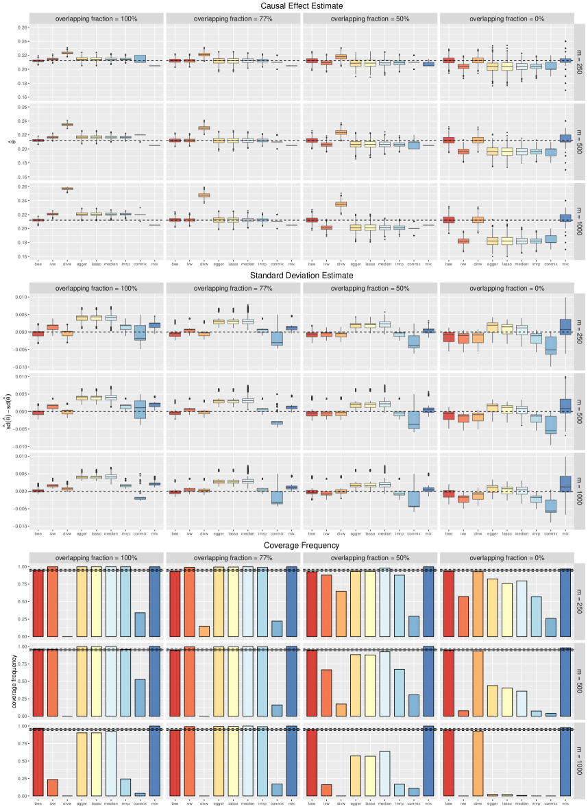
Figure 2: Investigation of MR methods for univarate MR with sample sizes $n_{0}=n_{1}=20000$, in terms of overlapping fraction and number of instrumental variants.

As for the standard error, we display the boxplot of $\hat{\text{se}}(\hat{\theta})-\text{se}(\hat{\theta})$ where $\text{se}(\hat{\theta})$ is approximated by the empirical SE calculated from the independent replications. It is evident that the SE estimates produced by all approaches have reduced variances as $m$ grows. However, only MRBEE and DIVW can provide consistent SE estimates, confirming the accuracy of MRBEE and DIVW’s SE formulas. Additionally, MR-ConMix is extremely likely to underestimate the standard error, while MR-Egger, MR-Lasso, MR-Median, and MR-Mix constantly overestimate it. As for IVW, it underestimates the SE when the fraction is large and overestimates it when the fraction is small.

The coverage frequency refers to the frequency that the confidence interval covers the true causal effect among simulations. Here, this confidence interval is constructed by doubling $\hat{\rm se}(\hat{\theta})$, which means that the coverage frequency corresponding to neither an inflated type-I error nor an inflated type-II error should be around 0.95. We observed that only MRBEE enjoys a coverage frequency around 0.95. When $m=250$, MR-Egger, MR-Lasso, and MR-Median suffer from inflated type-II error rates, likely because these methods cannot estimate the SE properly. These approaches also result in inflated-type I error rates caused by weak instrument bias as $m$ increases. Additionally, because MR-Mix overestimates the SE, it consistently exhibits a substantially inflated type-II error rate. Furthermore, IMRP and MR-ConMix consistently have inflated type I error rates because they frequently underestimate the SE.

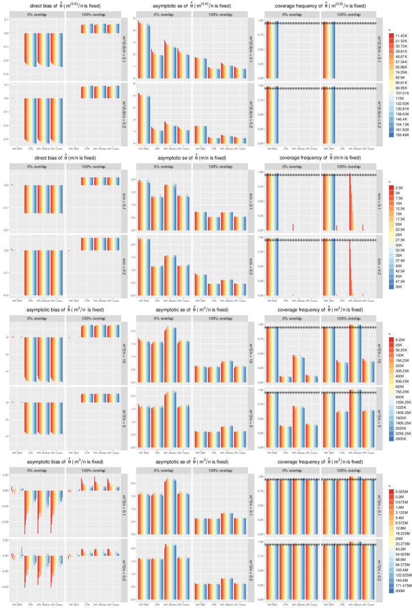
Figure 3: Investigations of MRBEE and IVW in terms of asymptotic bias and covariance matrix.

We next verify if the asymptotic normal distributions in Theorem 2 and Theorem 3 are correct. For a general estimate $\hat{\theta}$, the asymptotic bias and SE are $\sqrt{s}_{n}(\hat{\theta}-\theta)$ and $\sqrt{s}_{n}$se($\hat{\theta}$), respectively, where $\sqrt{s}_{n}$ is the convergence rate of $\hat{\theta}$. If this estimate is strongly asymptotically unbiased, the asymptotic bias $s_{n}(\hat{\theta}-\theta)$ should also be 0. Besides, if two estimates have equal asymptotic SEs, they are equally powerful in terms of statistical efficiency. We select MRBEE, IVW, MR-Median, and MR-Lasso to compare, only consider two overlapping fractions: 100% and 0%, set $n_{0}=n_{1}=n_{\rm min}$, and fix the causal effect $\theta=0.5$. As for $m$ and $n_{\rm min}$, we focus on the following four cases:

• $m=2500,5000,\dots,50000$ and $m^{0.9}/n=c_{0}=0.1$ and $0.2$; we examine the direct bias: $\hat{\theta}-\theta$, asymptotic SE: $\sqrt{n^{2}_{\rm min}/m}~{}{\rm se}(\hat{\theta})$, and coverage frequency;

• $m=250,500,\dots,5000$ and $m/n=c_{0}=0.1$ and $0.2$; we examine the direct bias: $\hat{\theta}-\theta$, asymptotic SE: $\sqrt{n}_{\rm min}~{}{\rm se}(\hat{\theta})$, and coverage frequency;

• $m=250,500,\dots,5000$ and $m^{2}/n=c_{0}=5$ and $10$; we examine the asymptotic bias: $\sqrt{n}_{\rm min}(\hat{\theta}-\theta)$, asymptotic SE: $\sqrt{n}_{\rm min}~{}{\rm se}(\hat{\theta})$, and coverage frequency;

• $m=250,500,\dots,5000$ and $m^{3}/n=c_{0}=5$ and $10$; we examine the asymptotic bias: $\sqrt{n}_{\rm min}(\hat{\theta}-\theta)$, asymptotic SE: $\sqrt{n}_{\rm min}~{}{\rm se}(\hat{\theta})$, and coverage frequency.

Note that we directly generate the estimation errors $\mathbf{W}_{\beta}$ and $\bm{w}_{\alpha}$ according to Theorem 1 because $n_{\rm min}$ in cases (3) and (4) can be larger than one million. The calculations involving individual-data are extremely time-consuming in these cases.

Figure 3 demonstrates the simulation results. In case (1), $\hat{\theta}_{\rm BEE}$ is unbiased while the other three estimates suffer from non-removable biases. As for the asymptotic SE, $\sqrt{n^{2}_{\rm min}/m}~{}{\rm se}(\hat{\theta}_{\rm BEE})$ remains unchanged when $n_{\rm min}$ and $m$ are sufficiently large (e.g., the bars colored in blue), verifying conclusion $(iii)$ in Theorem 3. However, the coverage frequency of MRBEE is a little larger than 0.95, meaning that the SE of $\hat{\theta}_{\rm BEE}$ is overestimated in this extreme case. This phenomenon is reasonable because Theorem 4 points out that the convergence rate of the sandwich formula is $\min(\sqrt{n}_{\rm min}$,$\sqrt{n_{\rm min}^{2}/m},\sqrt{m/\log m})$, which slows down as $m$ increases. In case (2), the direct bias of $\hat{\theta}_{\rm IVW}$ is unchanged as $n_{\rm min}$ tends to infinity, confirming conclusion $(iii)$ in Theorem 2. As for $\hat{\theta}_{\rm BEE}$, its asymptotic SE is a little larger than $\hat{\theta}_{\rm IVW}$, verifying item $(ii)$ in Theorem 3.

In case (3), the asymptotic bias of $\hat{\theta}_{\rm IVW}$ is constant as $n_{\rm min}$ goes to infinity, illustrating that $\hat{\theta}_{\rm IVW}$ is not strongly asymptotically unbiased. As a result, the coverage frequencies of $\hat{\theta}_{\rm IVW}$ are significantly smaller than 0.95, confirming our claim that any inference made based on $\hat{\theta}_{\rm IVW}$ is invalid. Besides, the asymptotic SEs of $\hat{\theta}_{\rm BEE}$ and $\hat{\theta}_{\rm IVW}$ are essentially the same, indicating that $\hat{\theta}_{\rm BEE}$ and $\hat{\theta}_{\rm IVW}$ are equally efficient as long as $m/n_{\rm min}\to 0$. In case (4), the asymptotic bias of IVW, MR-Median, and MR-Lasso vanish as $n_{\rm min}$ increases and their coverage frequencies are around 0.95, which is consistent with conclusion $(i)$ in Theorem 2. The equal asymptotic SEs also indicate that $\hat{\theta}_{\rm BEE}$ and $\hat{\theta}_{\rm IVW}$ are equally efficient in this scenario. In addition, IVW, MR-Median, and MR-Lasso suffer from the same degree of bias when there is no pleiotropy, while MR-Median not only suffers from a large asymptotic SE but also is likely to overestimate it. To understand why MR-Median is always less efficient than IVW when there is no pleiotropy, its asymptotic behavior is worthy of future investigation.

4.2 Multivariable MR investigation

For multivariable MR, we consider $p=6$ exposures and set the causal effect vector to be $\bm{\theta}=(0.3,0.3,-0.3,-0.3,0,0)^{\top}$. All of the exposures’ IV-heritabilities are 0.3, while the outcome’s IV-heritability is 0.15. We set an AR(1) structured genetic correlation matrix with coefficient $\rho=-0.5$ for the genetic effect $\bm{\beta}_{j}$, while considering a more intricate correlation structure for the noise terms $\bm{u}_{i}$ and $v_{i}$. In order to better mimic real data analysis, we take into account the scenario of completely overlapping GWAS samples (i.e., $n_{sk}=n_{s}=n_{k}$ for all $s,k$). Other cases of sample overlaps and details of the simulation settings are present in the supplementary materials.

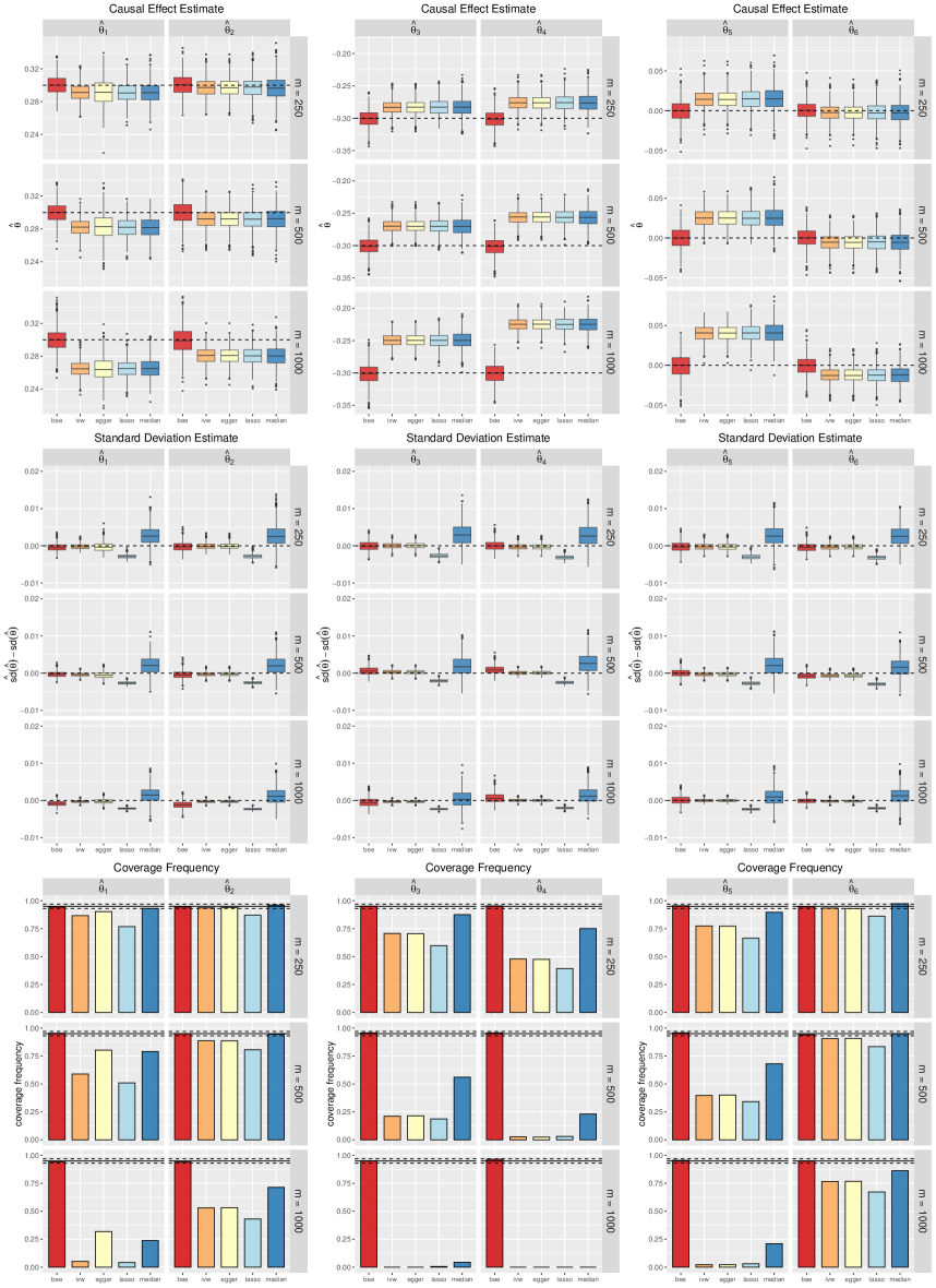
Figure 4: Investigation of MR methods for multivariable MR with sample sizes $n_{0}=\cdots=n_{6}=20000$ and overlap-sample sizes $n_{01}=\cdots=n_{65}=20000$, in terms of number of instrumental variants.

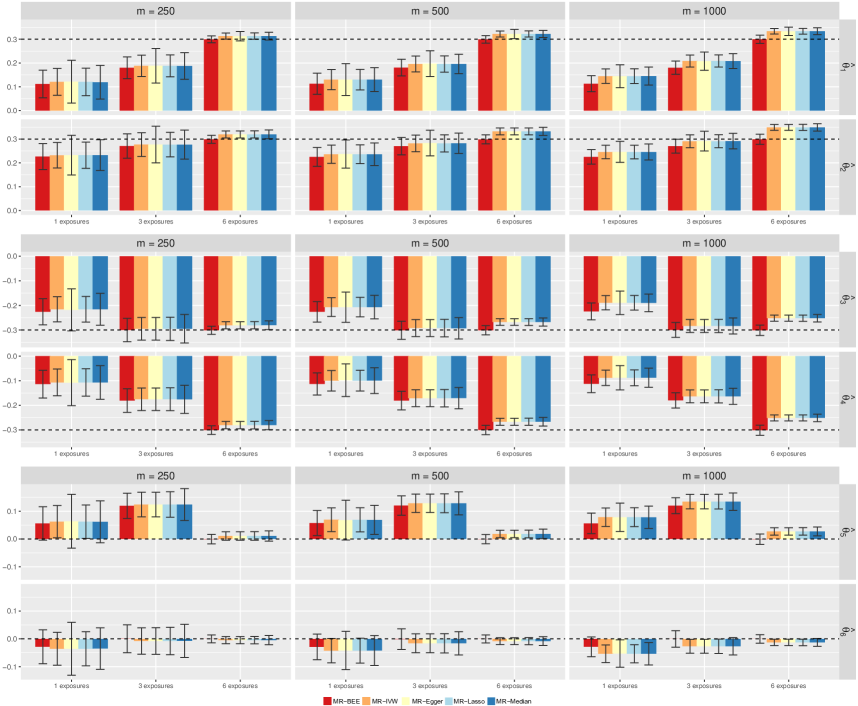
Figure 5: Investigation of MR methods for multivariable MR with sample sizes $n_{0}=\cdots=n_{6}=20000$ and overlap-sample sizes $n_{01}=\cdots=n_{65}=20000$, in terms of number of specified exposures.

Figure 4 presents the comparison between the multivariable versions of IVW, MR-Egger, MR-Lasso, MR-Median, and MRBEE. In general, MRBEE is the only method that can produce unbiased causal effect estimates in all cases. As $m$ increases, the SE of $\hat{\bm{\theta}}_{\rm BEE}$ remains the same, while the estimation error of the SE estimate becomes smaller. However, a very large $m$ may conversely reduce the accuracy of the SE estimate in multivariable MR. For example, the SE estimates of all approaches in the cases of $m=1000$ have larger empirical variances than those in the cases of $m=500$. This phenomenon can be explained by Theorem 5, which indicates that the convergence rate of the sandwich formula is $\min(\sqrt{n}_{\rm min}$,$\sqrt{n_{\rm min}^{2}/m},\sqrt{m/\log m})$. Hence, a larger $m$ may result in a worse SE estimate if $n_{\rm min}$ is not increased as $m$.

All the multivariable MR methods except MRBEE suffer from larger weak instrument biases with the increase of $m$. The SE estimates provided by these methods, in particular MR-Median, are less reliable than that of MRBEE. Thus, causal inferences based on the existing multivariable MR methods could be even more unreliable than univariable MR methods. In addition, $\hat{\bm{\theta}}_{\rm IVW}$ can have a bias toward any direction in multivariable MR. For example, the bias of $\hat{\theta}_{5,\rm IVW}$ is positive while the bias of $\hat{\theta}_{6,\rm IVW}$ is negative. The actual directions are jointly determined by the correlations of confounders and genetic effects.

We also examine the impact of omitting some important exposures. We conduct simulations when 1, 3, and all 6 exposures are included in the multivariable MR model, respectively. Figure 5 illustrates the results of the simulations. We observed that if associated exposures are omitted, the causal effect estimates can suffer severe biases. The degree of the biases is jointly determined by the genetic covariance matrix and covariance matrix of confounders. In conclusion, even though MRBEE has eliminated the estimation error bias and weak instrument bias, OVB still exists if any relevant exposure is not specified in the multivariable MR model.

4.3 Other Investigations

For univariable MR, we also investigated the effects of sample sizes, type-I error, winner’s curse, and outlier detection. Regarding multivariable MR, we investigated the impact of different sample overlaps. In addition, the precision of estimating $\bm{\Sigma}_{W_{\beta}w_{\alpha}}$ by insignificant GWAS statistics is also studied. Only by increasing the sample sizes of the exposure and outcome cohorts simultaneously, the accuracy of MRBEE can be improved. The traditional MR methods suffer from inflated type-I errors when the overlapping fraction is large. After accounting for the weak instrument bias and estimate error bias, MRBEE is almost free of the winner curse’s bias when the overlapping fraction is high. Furthermore, by applying the iterative method in IMRP, MRBEE can efficiently eliminate pleiotropic outliers and produce an accurate causal effect estimate. In addition, the estimation error $\bm{\Sigma}_{W_{\beta}w_{\alpha}}$ decreases with the increase of the number of insignificant variants $M$. Finally, multivariable MRBEE is accurate regardless of sample overlap. We summarized the findings with the simulation details in the supplementary material.

5 Real Data Analysis

Cardiovascular disease including coronary artery disease (CAD) is one of the leading causes of death for both men and women worldwide. There are many epidemiological studies and MR analyses based on GWAS summary data dedicated to identifying the causal risk factors for CAD. However, the causal effects of the risk factors on CAD are less clear and the existing evidence can be contradictory. For example, elevated low-density lipoprotein cholesterol level (LDL-C) is a well-established causal risk factor for CAD (Group et al., 1994), whereas Wang et al. (2022) concluded by multivariable MR analysis that LDL-C is not causally related to CAD in Europeans. Additionally, substantial observational analyses and molecular experiments have suggested that uric acid (UA) and red blood cell counts (RBC) contribute to the development of CAD (Bujak et al., 2015; Yu and Cheng, 2020). Nevertheless, Wang et al. (2022) did not observe significant causal effects of the two risk factors on CAD in Europeans. Furthermore, numerous MR analyses have concluded that body mass index (BMI) has a positive causal effect on CAD (Zhu, 2020; Wang et al., 2022). However, recent literature indicates that BMI is likely to influence CAD through the mediation with diseases such as diabetes and hypertension (Gill et al., 2021). These contradictions may be due to biases in MR methods, including OVB, weak instrument bias, estimation error bias, etc.

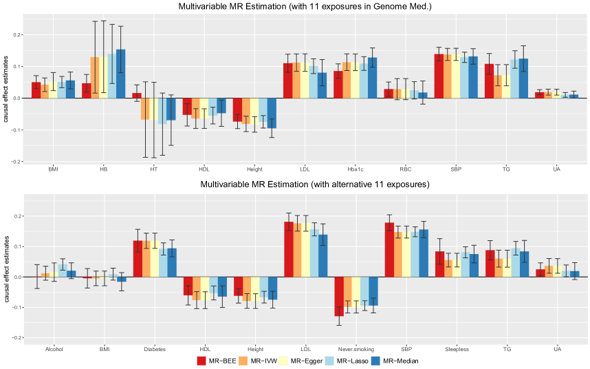
Figure 6: Causal effect estimates of CAD data. Confidence intervals are yielded by the double SE estimates.

We conducted two data analyses to estimate the causal effects of select risk factors on CAD. The first analysis uses the 11 exposures in Wang et al. (2022), including BMI, hemoglobin (HB), hemoglobin a1c (Hba1c), hematocrit (HT), high-density lipoprotein cholesterol level (HDL-C), height, LDL-C, RBC, systolic blood pressure (SBP), triglycerides (TG), and UA. In Wang et al. (2022), these 11 exposures were divided into two groups and analyzed separately. In contrast, we analyzed them in one multivariable MR model to avoid the OVB. In the second analysis, we replace HB, Hba1c, HT, and RBC with alcohol consumption (alcohol), diabetes, lifetime never smoking status (never.smoking), and sleeplessness. All the GWAS summary statistics used in our analyses were downloaded from the Neale lab (http://www.nealelab.is/uk-biobank/). Quality controls (QCs) are presented in the supplementary material. The total numbers of instrumental variants for the first and second analyses are 5345 and 5301, respectively.

Figure 6 displays the causal effect estimates with 95% confidence intervals. MRBEE confirms the causal effects of LDL-C, RBC, and UA on CAD. Here, HB, HT, and RBC have high mutual correlations: $\widehat{\text{cor}}(x_{\text{HB}},x_{\rm HT})=0.89$, $\widehat{\text{cor}}(x_{\text{HB}},x_{\rm RBC})=0.63$, and $\widehat{\text{cor}}(x_{\text{HT}},x_{\rm RBC})=0.72$, and thus the inferences obtained by the existing methods are not reliable. For example, the existing MR methods suggest that RBC is not significant, HB has a significant positive effect, and HT has a significant negative effect, which contradicts the fact that HT and CAD are positively associated (Sorlie et al., 1981). MRBEE corrects the estimation error bias and thus leads to a reasonable conclusion – HB and RBC have positive causal effects on CAD while HT has a positive but insignificant causal effect on CAD. For the second analysis, MRBEE reveals that BMI is likely to affect CAD through the mediation of SBP and diabetes. In addition, MRBEE indicates that never.smoking is protective against CAD, whereas sleeplessness is associated with increasing CAD risk. Furthermore, due to the weak instrument bias and estimation error bias, the existing methods overestimate the effects of HDL-C and height and underestimate the causal effects of diabetes, LDL-C, never.smoking, SBP, and sleeplessness. By using MRBEE, we are able to obtain reliable causal effect estimates and therefore make valid inferences on the causal risk factors of CAD.

6 Discussion

In this paper, we first investigated the asymptotic behavior of the multivariable IVW estimate. Since almost all MR methods are based on the IVW method, understanding the asymptotic behavior of the IVW estimate has very far-reaching implications for the theoretical and empirical studies of MR methods. We found that the bias of the multivariable IVW estimate is the product of weak instrument bias and estimation error bias. Also, we revealed that estimation error bias is a linear combination of measurement error bias and confounder bias, in which the sample overlaps trade off the proportion of these two components of estimation error bias. In the literature, although the phenomenon that the IVW estimate suffers from bias has been observed, a quantitative explanation for its existence is still absent. Our work fills the gap, which is a significant theoretical contribution to MR.

Subsequently, in this paper, we describe MRBEE that can yield the unbiased causal effect estimate $\hat{\bm{\theta}}_{\rm BEE}$. We point out that $\hat{\bm{\theta}}_{\rm BEE}$ is strongly asymptotically unbiased in all scenarios, indicating that $\hat{\bm{\theta}}_{\rm BEE}$ is asymptotically valid when making causal inferences. We also discuss how to perform MRBEE in practice, including how to estimate the bias-correction terms, how to estimate the sandwich formula, and how to identify possible UHP when multiple exposures are included. We present corresponding theorems to confirm that the estimates involved in the implementation of MRBEE are consistent in theory. In simulations, we show that MRBEE simultaneously estimates causal effects and the SE unbiasedly, and identifies UHP consistently. In section 5 and also in (Lorincz-Comi et al., 2022), the practical advances of MRBEE are further demonstrated.

It is worth offering guidance on how to properly perform MR analysis from our perspective. First, we suggest applying the multivariable MR approach instead of the univariable MR approach because the causal effect estimates obtained by the univariable MR approach are unreliable due to OVB, regardless of the presence of UHP and CHP in the model. Second, rather than selecting the optimal number of instrumental variants such that the F statistics and conditional F statistics are larger than 10 (Burgess et al., 2011; Sanderson et al., 2021), we advise including all the independent instrumental variants that are significantly associated with one or more exposures. Our theory illustrates that the asymptotic variance of a causal effect estimate is related to the cumulative variance explained by all specified IVs instead of the average variance explained by each IV. In particular, there is no need to worry about the issue of weak IVs because MRBEE has demonstrated efficiency to eliminate weak instrument bias through our simulations and theory. Third, when performing multivariable MR analysis, it is not necessary to remove variants that are pleiotropic between the exposures. For example, Wang et al. (2022) observed that LDL-C was insignificantly associated with CAD in Europeans, which is unlikely to be true because this risk causality has been well established in randomized clinical trials (Group et al., 1994). The potential reason for this false negative is that Wang et al. (2022) excluded the IVs associated with RBC, HB, HT, and UA in their multivariable MR analysis. We believe that the proper way to perform multivariable MR analysis is to simultaneously include all the relevant exposures, as the multivariable regression can automatically account for the pleiotropic variants shared by the specified exposures. Fourth, among the existing multivariable MR approaches including IVW, MR-Egger, and MR-Lasso, we recommend MRBEE as the primary analysis approach because it has been proven to be the only one that enjoys strongly asymptotic unbiasedness in the presence of many weak IVs.

Appendix A Proof

A.1 Preliminary lemmas

In this subsection, we specify some lemmas that can facilitate the proofs, most of which can be found in the existing papers. We first discuss the equivalent characterizations of sub-Gaussian and sub-exponential variables.

Lemma A.1 (Equivalent characterizations of sub-Guassian variables).

Given any random variable $X$, the following properties are equivalent:

• there is a constant $K_{1}\geq 0$ such that

  $$\Pr(|X|\geq t)\leq 2\exp(-t^{2}/K_{1}^{2}),\quad\text{for all }t\geq 0,$$

• the moments of $X$ satisfy

  $$||X||_{L_{p}}=(\text{E}(|X|^{p}))^{\frac{1}{p}}\leq K_{2}\surd p,\quad\text{for all }p\geq 1,$$

• the moment generating function (MGF) of $X^{2}$ satisfies:

  $$\text{E}\{\exp(\lambda^{2}X^{2})\}\leq\exp(K_{3}^{2}\lambda^{2}),\quad\text{for all $\lambda$ staisfying }|\lambda|\leq K_{3}^{-1},$$

• the MGF of $X^{2}$ is bounded at some point, namely

  $$\text{E}\{\exp(X^{2}/K_{4}^{2})\}\leq 2,$$

• if E$(X)=0$, the MGF of $X$ satisfies

  $$\text{E}\{\exp(\lambda X)\}\leq\exp(K_{5}^{2}\lambda^{2}),\quad\text{for all }\lambda\in\mathbb{R},$$

where $K_{1},\dots,K_{5}$ are certain strictly positive constants.

This lemma summarizes some well-known properties of sub-Guassian and can be found in Vershynin (2018, Proposition 2.5.2).

Lemma A.2 (Equivalent characterizations of sub-exponential variables).

Given any random variable $X$, the following properties are equivalent:

• there is a constant $K_{1}\geq 0$ such that

  $$\Pr(|X|\geq t)\leq 2\exp(-t/K_{1}),\quad\text{for all }t\geq 0,$$

• the moments of $X$ satisfy

  $$||X||_{L_{p}}=(\text{E}(|X|^{p}))^{\frac{1}{p}}\leq K_{2}p,\quad\text{for all }p\geq 1,$$

• the moment generating function (MGF) of $|X|$ satisfies:

  $$\text{E}\{\exp(\lambda|X|)\}\leq\exp(K_{3}\lambda),\quad\text{for all $\lambda$ staisfying }0\leq\lambda\leq K_{3}^{-1},$$

• the MGF of $|X|$ is bounded at some point, namely

  $$\text{E}\{\exp(|X|/K_{4})\}\leq 2,$$

• if E$(X)=0$, the MGF of $X$ satisfies

  $$\text{E}\{\exp(\lambda X)\}\leq\exp(K_{5}^{2}\lambda^{2}),\quad\text{for all }\lambda\leq K_{5}^{-1},$$

where $K_{1},\dots,K_{5}$ are certain strictly positive constants.

This lemma summarizes some well-known properties of sub-exponential and can be found in Vershynin (2018, Proposition 2.7.1).

Lemma A.3 (Product of sub-Gaussian variable is sub-exponential).

Suppose that $X,Z$ are two sub-Gaussian variable, then $Y=XZ$ is a sub-exponential variable. Besides, if $X$ is a bounded sub-Gaussian variable, then then $Y=XZ$ is a sub-Gaussian variable.

The first claim of this lemma is provided by Vershynin (2018, Proposition 2.7.7). The second claim of this lemma is a direct inference of Fan et al. (2011, Lemma A.2).

Lemma A.4 ($\ell_{2}$-norm of matrices with sub-Gaussian entries).

Let $\bm{X}_{1},\dots,\bm{X}_{n}$ be $n$ $(p\times 1)$ independent identically distributed random vector with entries $x_{i1},\dots,x_{ip}$ are sub-Gaussian with zero-mean. Besides, define the covariance matrix of $\bm{X}_{i}$ as

$$\bm{\Sigma}=\text{E}(\bm{X}_{i}\bm{X}_{i}^{\top})$$

and the related sample covariance matrix

$$\hat{\bm{\Sigma}}=\frac{1}{n}\sum_{i=1}^{n}\bm{X}_{i}\bm{X}_{i}^{\top}.$$

Then for every positive integer $n$,

$$\text{E}(||\hat{\bm{\Sigma}}-\bm{\Sigma}||_{2})\leq C\bigg{(}\frac{p}{n}+\sqrt{\frac{p}{n}}\bigg{)}||\bm{\Sigma}||_{2},$$

where $C$ is certain positive constant.

This lemma is provided by Vershynin (2018, Theorem 4.7.1). It shows the convergence rate of sample covariance matrix is $\surd(n/m)$.

Lemma A.5 ($\ell_{2}$-norm of matrices with sub-exponential entries).

Let $\bm{X}_{1},\dots,\bm{X}_{n}$ be $n$ $(p\times 1)$ independent identically distributed random vector with entries $x_{i1},\dots,x_{ip}$ are sub-exponential with zero-mean. Besides, define the covariance matrix of $\bm{X}_{i}$ as

$$\bm{\Sigma}=\text{E}(\bm{X}_{i}\bm{X}_{i}^{\top})$$

and the related sample covariance matrix

$$\hat{\bm{\Sigma}}=\frac{1}{n}\sum_{i=1}^{n}\bm{X}_{i}\bm{X}_{i}^{\top}.$$

Then for ever $t\geq 0$, the following inequality holds with probability at least $1-p\exp(-ct^{2})$:

$$||\hat{\bm{\Sigma}}-\bm{\Sigma}||_{2}\leq\max(||\bm{\Sigma}||_{2}\delta,\delta^{2}),$$

where $c$ is certain positive constant and $\delta=t\sqrt{p/n}$.

This lemma is the direct inference of Vershynin (2010, Theorem 5.44). Besides, by letting $t=\sqrt{p\log n}$ we further obtain

$$\text{E}(||\hat{\bm{\Sigma}}-\bm{\Sigma}||_{2})=O\bigg{(}\sqrt{\frac{p\log n}{n}}\bigg{)}||\bm{\Sigma}||_{2},$$

if $\hat{\bm{\Sigma}}$ is the sample covariance matrix of sub-exponential vector. Note that in our method, the dimension $p$ is fixed and hence we cannot chose $t=\sqrt{p\log p}$ such that the estimation bound becomes $\sqrt{(p\log p)/n}||\bm{\Sigma}||_{2}$.

Lemma A.6 (Asymptotic normal distribution of Wishart matrix).

Suppose $\bm{X}_{1},\bm{X}_{2},\dots,\bm{X}_{n}$ are $n$ IID relaxation of the $p$-dimensional variable $\bm{X}\sim\mathcal{N}(\mathbf{0},\bm{\Sigma})$ with a well-conditioned covariance matrix $\bm{\Sigma}$. Besides, define the sample covariance matrix of $\bm{\Sigma}$ as

$$\hat{\mathbf{\Sigma}}=\frac{1}{n}\sum_{i=1}^{n}\bm{X}_{i}\bm{X}_{i}^{\top}.$$

If $p$ is a fixed number, then as $n\to\infty$,

$$\sqrt{n}(\text{vec}(\hat{\mathbf{\Sigma}})-\text{vec}(\bm{\Sigma}))\stackrel{{\scriptstyle D}}{{\longrightarrow}}\mathcal{N}\bigg{(}\mathbf{0},(\mathbf{I}_{p^{2}}+\mathbf{K}_{p^{2}})(\bm{\Sigma}\otimes\bm{\Sigma})\bigg{)},$$

where $\mathbf{K}_{p^{2}}$ is the so-called commutation matrix, which is able to ensure $\mathbf{K}_{p^{2}}\text{vec}(\mathbf{A})=\text{vec}(\mathbf{A}^{\prime})$ for all $(p\times p)$ matrix.

This lemma can be found in Muirhead (2009, equation (5), p90).

A.2 Specific Lemmas

In this subsection, we specify the following lemmas that are made based on the preliminary lemmas.

Lemma A.7 (Asymptotic normal distribution of sub-Gaussian and sub-exponential variables).

Suppose $X_{1},\dots,X_{n}$ are $n$ independent sub-Gaussian or sub-exponential variables with mean-zero and variance $\sigma_{1}^{2},\dots,\sigma_{n}^{2}$ . Then

$$\lim_{n\to\infty}\frac{1}{\sqrt{n}}\sum_{i=1}^{n}X_{i}\stackrel{{\scriptstyle D}}{{\longrightarrow}}\mathcal{N}(0,\sigma_{x}^{2}),$$

where

$$\sigma_{x}^{2}=\lim_{n\to\infty}\frac{1}{n}\sum_{i=1}^{n}\sigma_{i}^{2}.$$

Proof of Lemma A.7.

It is easy to verify the Lyapunov’s condition: for all fixed $\delta>0$,

$$\lim_{n\to\infty}\frac{1}{n^{1+\delta}}\sum_{i=1}^{n}\text{E}(|X_{i}|^{2+2\delta})\leq\frac{\sqrt{2K_{2}+2K_{2}\delta}^{2+2\delta}}{n^{\delta}}\to 0$$

by the (II) of Lemma A.1, if $X_{1},\dots,X_{n}$ are sub-Gaussian variables;

$$\lim_{n\to\infty}\frac{1}{n^{1+\delta}}\sum_{i=1}^{n}\text{E}(|X_{i}|^{2+2\delta})\leq\frac{(2K_{2}+2K_{2}\delta)^{2+2\delta}}{n^{\delta}}\to 0$$

by the (II) of Lemma A.2, if $X_{1},\dots,X_{n}$ are sub-exponential variables. And hence the asymptotic normal distribution holds. ∎

Lemma A.8 (Asymptotic normal distribution of estimation error).

Let

$$\xi_{j}^{[s]}=\frac{1}{\sqrt{n_{s}}}\sum_{i=1}^{n_{s}}g^{[s]}_{ij}x^{[s]}_{i,-j},$$

where

$$x^{[s]}_{i,-j}=x^{[s]}_{i}-\beta_{js}g^{[s]}_{i,j},$$

$s=0,1,\dots,p$, $x_{i,-j}^{[0]}$ represents $y_{i,-j}^{[0]}$ and $\beta{j0}$ represent $\alpha_{j}$. Then

$$\xi^{[s]}_{j}\xrightarrow{D}\mathcal{N}(0,\sigma_{x_{s}x_{s}}-\sigma_{\beta_{s}\beta_{s}}),$$

where $\sigma_{x_{0}x_{0}}$ represents $\sigma_{yy}$ and $\sigma_{\beta_{0}\beta_{0}}$ represents $\bm{\theta}^{\top}\bm{\Sigma}_{\beta\beta}\theta$.

Proof of Lemma A.8.

Note that both $g^{[s]}_{ij}$ and $x^{[s]}_{i,-j}$ are sub-Gaussian ($x^{[s]}_{i,-j}$ is the product of a sub-Gaussian variable and a bounded sub-Gaussian variable), and it holds E$(g^{[s]}_{ij}x^{[s]}_{i,-j})=0$ and

$$\text{var}(g^{[s]}_{ij}x^{[s]}_{i,-j})=\text{var}(g^{[s]}_{ij})\times\text{var}(x^{[s]}_{i,-j})=\sigma_{x_{s}x_{s}}-\sigma_{\beta_{s}\beta_{s}}.$$ (32)

As a result,

$$\xi^{[s]}_{j}=\frac{1}{\sqrt{n_{s}}}\sum_{i=1}^{n_{s}}g^{[s]}_{ij}x^{[s]}_{i,-j}\xrightarrow{D}\mathcal{N}(0,\sigma_{x_{s}x_{s}}-\sigma_{\beta_{s}\beta_{s}}),$$ (33)

according Lemma A.7. ∎

Lemma A.9 (Asymptotic normality of bias-correction terms).

Let

$$\bm{\zeta}_{j}=\bigg{(}\frac{n_{\rm min}}{n_{1}}\xi^{[1]}_{j},\frac{n_{\rm min}}{n_{2}}\xi^{[2]}_{j},\dots,\frac{n_{\rm min}}{n_{p}}\xi^{[p]}_{j},\frac{n_{\rm min}}{n_{0}}\xi^{[0]}_{j}\bigg{)}^{\top}.$$

Under the conditions (C1)-(C4),

$$\lim_{m\to\infty}\frac{1}{\sqrt{m}}\sum_{j=1}^{m}(\text{vec}(\bm{\zeta}_{j}\bm{\zeta}_{j}^{\top})-\text{vec}(\bm{\Psi}_{W_{\beta}\times w_{\alpha}}))\xrightarrow{D}\mathcal{N}\bigg{(}\mathbf{0},(\mathbf{I}_{p^{2}}+\mathbf{K}_{p^{2}})(\bm{\Psi}_{W_{\beta}\times w_{\alpha}}\otimes\bm{\Psi}_{W_{\beta}\times w_{\alpha}})\bigg{)}.$$

as $n_{\rm min},m\to\infty$.

Proof of Lemma A.9.

By using Lemma A.7, $\bm{\zeta}_{j}$ follows $\mathcal{N}(0,\bm{\Psi}_{W_{\beta}\times w_{\alpha}})$ as $n_{\rm min}\to\infty$. Then by using Lemma A.6, this lemma holds. ∎

Lemma A.10 (Asymptotic normality of residual term).

Under the conditions (C1)-(C4),

$$\lim_{m\to\infty}\frac{1}{\sqrt{m}}\sum_{j=1}^{m}\sqrt{m}\bm{\beta}_{j}\xi_{j}^{[s]}\xrightarrow{D}\mathcal{N}(0,\sigma_{x_{s}x_{s}}\bm{\Sigma}_{\beta\beta}),$$

and

$$\lim_{m\to\infty}\frac{1}{m}\sum_{j=1}^{m}\sqrt{m}\bm{\beta}_{j}\sqrt{m}\bm{\beta}_{j}^{\top}\xi_{j}^{[s]}\xi_{j}^{[k]}\xrightarrow{P}\frac{n_{sk}}{\sqrt{n_{s}n_{k}}}\sigma_{x_{s}x_{k}}\bm{\Sigma}_{\beta\beta},$$

for $s=0,\dots,p$, where $\sigma_{x_{0}x_{k}}$ represents $\sigma_{yx_{k}}=\sum_{l=1}^{p}\theta_{l}\sigma_{x_{l}x_{k}}$.

Proof of Lemma A.10.

By condition (C4), $\sqrt{m}\bm{\beta}_{j}$ is independent of $\xi_{j}^{[s]}$. By Lemma A.3, $\sqrt{m}\bm{\beta}_{j}\xi_{j}^{[s]}$ is sub-exponential with mean $\mathbf{0}$ and covariance matrix

$$\text{cov}(\sqrt{m}\bm{\beta}_{j}\xi_{j}^{[s]}) =\text{cov}(\sqrt{m}\bm{\beta}_{j})\times\text{var}(\xi_{j}^{[s]})$$

$$=(\sigma_{x_{s}x_{s}}-\sigma_{\beta_{s}\beta_{s}})\bm{\Sigma}_{\beta\beta}.$$ (34)

Hence, by Lemma A.6,

$$\lim_{m\to\infty}\frac{1}{\sqrt{m}}\sum_{j=1}^{m}\sqrt{m}\bm{\beta}_{j}\xi_{j}^{[s]}\xrightarrow{D}\mathcal{N}(0,\sigma_{x_{s}x_{s}}\bm{\Sigma}_{\beta\beta}).$$

On the other hand, $\bm{\beta}_{j}\xi_{j}^{[s]}$ is sub-exponential variable according to Lemma A.3, and

$$\text{cov}(\sqrt{m}\bm{\beta}_{j}\xi_{j}^{[s]},\sqrt{m}\bm{\beta}_{j}\xi_{j}^{[k]}) =\text{cov}(\xi_{j}^{[s]},\xi_{j}^{[k]})\times\bm{\Sigma}_{\beta\beta}$$

$$=\frac{n_{sk}}{\sqrt{n_{s}n_{k}}}(\sigma_{x_{s}x_{k}}-\sigma_{\beta_{s}\beta_{k}})\bm{\Sigma}_{\beta\beta}.$$ (35)

Hence, by using Lemma A.5

$$\lim_{m\to\infty}\frac{1}{m}\sum_{j=1}^{m}\sqrt{m}\bm{\beta}_{j}\sqrt{m}\bm{\beta}_{j}^{\top}\xi_{j}^{[s]}\xi_{j}^{[k]}\xrightarrow{P}\frac{n_{sk}}{\sqrt{n_{s}n_{k}}}\sigma_{x_{s}x_{k}}\bm{\Sigma}_{\beta\beta}.$$

∎

A.3 Proofs of theorems in section 2

Proof of Theorem 1.

As for the estimation error $\bm{\omega}_{\alpha}$, we have

$$w_{\alpha_{j}}=\frac{\bm{g}_{j}^{[0]\top}\bm{y}^{[0]}}{n_{0}}-\alpha_{j}=\frac{\bm{g}_{j}^{[0]\top}\bm{y}^{[0]}_{-j}}{n_{0}},$$ (36)

where

$$\bm{y}^{[0]}_{-j}=\bm{y}^{[0]}-\alpha_{j}\bm{g}_{j}^{[0]}=\sum_{s\neq j}^{m}\alpha_{t}\bm{g}_{t}^{[0]}+\mathbf{U}^{[0]}\bm{\theta}+\bm{v}^{[0]},$$ (37)

and $\mathbf{U}^{[0]}$ and $\bm{v}^{[0]}$ are the corresponding noise terms in the outcome GWAS cohort. According to Lemma A.8,

$$\xi^{[0]}_{j}=\frac{1}{\sqrt{n_{0}}}\sum_{i=1}^{n_{0}}g^{[0]}_{ij}y^{[0]}_{i,-j}\xrightarrow{D}\mathcal{N}(0,\sigma_{yy}-\bm{\theta}^{\top}\bm{\Sigma}_{\beta\beta}\bm{\theta}).$$ (38)

As for the estimation error $w_{\beta_{js}}$, we have

$$w_{\beta_{js}}=\frac{\bm{g}_{j}^{[s]\top}\bm{x}^{[s]}}{n_{s}}-\beta_{js}=\frac{\bm{g}_{j}^{[s]\top}\bm{x}^{[s]}_{-j}}{n_{s}},$$ (39)

where

$$\bm{x}^{[s]}_{-j}=\bm{x}^{[s]}-\bm{g}_{j}^{[s]}\beta_{js}=\sum_{t\neq j}\beta_{ts}\bm{g}_{t}^{[s]}+\bm{u}^{[s]}.$$ (40)

Let

$$\xi_{j}^{[s]}=\frac{\bm{g}_{j}^{[s]\top}\bm{x}^{[s]}_{-j}}{\sqrt{n_{s}}}=\frac{1}{\sqrt{n}_{s}}\sum_{i=1}^{n_{s}}g_{ij}^{[s]}x_{i,-j}^{[s]},$$ (41)

where $x_{i,-j}^{[s]}$ is the $i$th element in vector $\bm{x}^{[s]}_{-j}$. According to Lemma A.8,

$$\xi_{j}^{[s]}=\frac{1}{\sqrt{n}_{s}}\sum_{i=1}^{n_{s}}g_{ij}^{[s]}x_{i,-j}^{[s]}\xrightarrow{D}\mathcal{N}(0,\sigma_{x_{s}x_{s}}-\sigma_{\beta_{s}\beta_{s}}).$$ (42)

Now we show the covariance between $\xi^{[s]}_{j}$ and $\xi^{[k]}_{j}$:

$$\text{cov}(\xi^{[s]}_{j},\xi^{[k]}_{j})=\text{E}\bigg{(}\frac{\bm{x}_{-j}^{[s]\top}\bm{g}_{j}^{[s]}\bm{g}_{j}^{[k]\top}\bm{x}_{-j}^{[k]}}{\sqrt{n_{s}n_{k}}}\bigg{)},$$ (43)

where $\bm{x}_{-j}^{[0]}$ represents $\bm{y}_{-j}^{[0]}$ for simplicity. Denote $\mathbf{Q}^{[sk]}=(Q_{it}^{[sk]})$ being a $(n_{s}\times n_{k})$ matrix whose $(i,t)$th element is

$$Q^{[sk]}_{it}=\text{E}(g_{ij}^{[s]}g_{tj}^{[k]})=\begin{cases}1,&(i,t)\in\mathcal{Q}^{[sk]},\\ 0,&(i,t)\notin\mathcal{Q}^{[sk]},\end{cases}$$ (44)

where

$$\mathcal{Q}^{[sk]}=\{(i,t):\ g_{ij}^{[s]}\text{ and }g_{tj}^{[k]}\text{ come from the same individual}\}.$$ (45)

As a result,

$$\text{cov}(\xi^{[s]}_{j},\xi^{[k]}_{j}) =\text{E}\bigg{(}\frac{\bm{x}_{-j}^{[s]\top}\mathbf{Q}^{[sk]}\bm{x}_{-j}^{[k]}}{\sqrt{n_{s}n_{k}}}\bigg{)}=\frac{1}{\sqrt{n_{s}n_{k}}}\sum_{(i,t)\in\mathcal{Q}^{[sk]}}\text{E}(x_{i,-j}^{[s]}x_{t,-j}^{[k]})$$

$$=\frac{n_{sk}}{\sqrt{n_{s}n_{k}}}\bigg{(}\sigma_{x_{s}x_{k}}-\sigma_{\beta_{s}\beta_{k}}\bigg{)},$$ (46)

where $\sigma_{x_{0}x_{k}}$ represents $\sigma_{yx_{k}}$ for simplicity, and $\sigma_{\beta_{0}\beta_{k}}$ represents

$$\sigma_{\beta_{0}\beta_{k}}=\text{cov}(\sqrt{m}\bm{\beta}_{j}^{\top}\bm{\theta},\sqrt{m}\beta_{jk})=\sum_{l=1}^{p}\theta_{l}\sigma_{\beta_{l}\beta_{k}}.$$ (47)

Finally, we show $\xi^{[s]}_{j}$ is uncorrelated with $\xi^{[s]}_{t}$ for all $t\neq j$ and $s=0,\dots,p$. Specifically,

$$\text{cov}(\xi^{[s]}_{j},\xi^{[s]}_{t})=\text{E}\bigg{(}\frac{\bm{x}_{-j}^{[s]\top}\bm{g}_{j}^{[s]}\bm{g}_{t}^{[s]\top}\bm{x}_{-j}^{[s]}}{n_{s}}\bigg{)}.$$ (48)

According the model setting, $\bm{g}_{j}^{[s]}$ is independent of $\bm{g}_{t}^{[s]}$ for all $t\neq s$. Therefore, $\text{cov}(\xi^{[s]}_{j},\xi^{[s]}_{t})=0$.

Note that if $m\to\infty$, $\bm{\Sigma}_{\beta\beta}=\frac{1}{m}\mathbf{\Psi}_{\beta\beta}$ vanishes. And so Theorem 1 is proved. ∎

Proof of Theorem 2.

The score function of IVW is

$$-\frac{1}{m}\hat{\mathbf{B}}^{\top}(\bm{\hat{a}}-\hat{\mathbf{B}}\hat{\bm{\theta}}_{\rm IVW})=-\frac{1}{m}\hat{\mathbf{B}}^{\top}(\bm{\hat{a}}-\hat{\mathbf{B}}\bm{\theta})+\frac{1}{m}\hat{\mathbf{B}}^{\top}\hat{\mathbf{B}}(\hat{\bm{\theta}}_{\rm IVW}-\bm{\theta})$$ (49)

which leads to

$$\mathbf{H}_{\rm IVW}(\hat{\bm{\theta}}_{\rm IVW}-\bm{\theta})=-\bm{S}_{\rm IVW}(\bm{\theta}),$$ (50)

where

$$\mathbf{H}_{\rm IVW}=\frac{1}{m}\hat{\mathbf{B}}^{\top}\hat{\mathbf{B}},\quad\bm{S}_{\rm IVW}(\bm{\theta})=-\frac{1}{m}\hat{\mathbf{B}}^{\top}(\bm{\hat{a}}-\hat{\mathbf{B}}\bm{\theta}).$$ (51)

We first work with the Hessian matrix $\mathbf{H}_{\rm IVW}$:

$$m\mathbf{H}_{\rm IVW} =\hat{\mathbf{B}}^{\top}\hat{\mathbf{B}}=\mathbf{B}^{\top}\mathbf{B}+\mathbf{B}^{\top}\mathbf{W}_{\beta}+\mathbf{W}_{\beta}^{\top}\mathbf{B}+\mathbf{W}_{\beta}^{\top}\mathbf{W}_{\beta}$$

$$=\mathbf{J}_{1}+\mathbf{J}_{2}+\mathbf{J}_{3}+\mathbf{J}_{4}.$$ (52)

As for $\mathbf{J}_{1}$,

$$\mathbf{J}_{1}=\sum_{j=1}^{m}\bm{\beta}_{j}\bm{\beta}_{j}^{\top}\stackrel{{\scriptstyle P}}{{\longrightarrow}}\bm{\Psi}_{\beta\beta}.$$ (53)

As for $\mathbf{J}_{2}$,

$$\|\sqrt{n}_{\rm min}\mathbf{J}_{2}\|_{2} =\bigg{\|}\frac{1}{\sqrt{m}}\sum_{j=1}^{m}(\sqrt{n}_{\rm min}\bm{w}_{\beta_{j}})(\sqrt{m}\bm{\beta}_{j})^{\top}\bigg{\|}_{2}$$

$$\leq\sqrt{\bigg{\|}\frac{1}{m}\sum_{j=1}^{m}(\sqrt{n}_{\rm min}\bm{w}_{\beta_{j}})(\sqrt{n}_{\rm min}\bm{w}_{\beta_{j}})^{\top}\bigg{\|}_{2}}\times\sqrt{\bigg{\|}\frac{1}{m}\sum_{j=1}^{m}(\sqrt{m}\bm{\beta}_{j})(\sqrt{m}\bm{\beta}_{j})^{\top}\bigg{\|}_{2}}$$

$$\leq\lambda_{\max}^{\frac{1}{2}}(\bm{\Psi}_{W_{\beta}W_{\beta}})\times\lambda_{\max}^{\frac{1}{2}}(\bm{\Psi}_{\beta\beta}),$$ (54)

which means

$$\|\mathbf{J}_{2}\|_{2}=O_{P}(1/\sqrt{n}_{\rm min}).$$ (55)

As for $\mathbf{J}_{3}$, it has the same order as $\mathbf{J}_{2}$. As for $\mathbf{J}_{4}$,

$$\frac{n_{\rm min}}{m}\mathbf{J}_{4}=\frac{1}{m}\sum_{j=1}^{m}(\sqrt{n}_{\rm min}\bm{w}_{\beta_{j}})(\sqrt{n}_{\rm min}\bm{w}_{\beta_{j}})^{\top}\stackrel{{\scriptstyle P}}{{\longrightarrow}}\bm{\Psi}_{W_{\beta}W_{\beta}}$$ (56)

Hence:

• If $m/n_{\rm min}\to 0$,

  $$\|\mathbf{J}_{4}\|_{2}\leq\lambda_{\max}(\bm{\Psi}_{W_{\beta}W_{\beta}})\times\frac{m}{n_{\rm min}}\to 0.$$ (57)

  Therefore,

  $$m\mathbf{H}_{\rm IVW}\stackrel{{\scriptstyle P}}{{\longrightarrow}}\bm{\Psi}_{\beta\beta}.$$ (58)

• If $m/n_{\rm min}\to c_{0}\in(0,\infty)$, then

  $$\mathbf{J}_{4}=\frac{m}{n_{\rm min}}\times\frac{1}{m}\sum_{j=1}^{m}(\sqrt{n}_{\rm min}\bm{w}_{\beta_{j}})(\sqrt{n}_{\rm min}\bm{w}_{\beta_{j}})^{\top}\stackrel{{\scriptstyle P}}{{\longrightarrow}}c_{0}\bm{\Psi}_{W_{\beta}W_{\beta}}.$$ (59)

  Therefore,

  $$m\mathbf{H}_{\rm IVW}\stackrel{{\scriptstyle P}}{{\longrightarrow}}\bm{\Psi}_{\beta\beta}+c_{0}\bm{\Psi}_{W_{\beta}W_{\beta}}.$$ (60)

• If $m/n_{\rm min}\to\infty$ and $m/n_{\rm min}^{1+\tau}\to c_{0}\in(0,+\infty)$ with certain constant $\tau>0$, then

  $$\frac{1}{n_{\rm min}^{\tau}}\mathbf{J}_{4}=\frac{m}{n_{\rm min}^{1+\tau}}\times\frac{1}{m}\sum_{j=1}^{m}(\sqrt{n}_{\rm min}\bm{w}_{\beta_{j}})(\sqrt{n}_{\rm min}\bm{w}_{\beta_{j}})^{\top}\stackrel{{\scriptstyle P}}{{\longrightarrow}}c_{0}\bm{\Psi}_{W_{\beta}W_{\beta}}.$$ (61)

  Therefore,

  $$\frac{m}{n_{\rm min}^{\tau}}\mathbf{H}_{\rm IVW}=c_{0}n_{\rm min}\mathbf{H}_{\rm IVW}\stackrel{{\scriptstyle P}}{{\longrightarrow}}c_{0}\bm{\Psi}_{W_{\beta}W_{\beta}}.$$ (62)

We then work with $\bm{S}_{\rm IVW}(\theta)$:

$$m\bm{S}_{\rm IVW}(\theta) =-\mathbf{B}^{\top}\bm{w}_{\alpha}-\mathbf{W}_{\beta}^{\top}\bm{w}_{\alpha}+\mathbf{B}^{\top}\mathbf{W}_{\beta}\bm{\theta}+\mathbf{W}_{\beta}^{\top}\mathbf{W}_{\beta}\bm{\theta}$$

$$=\bm{K}_{1}+\bm{K}_{2}+\bm{K}_{3}+\bm{K}_{4}.$$ (63)

As for $\bm{K}_{1}+\bm{K}_{3}$,

$$\sqrt{n}_{\rm min}(\bm{K}_{1}+\bm{K}_{3})=\frac{1}{\sqrt{m}}\sum_{j=1}^{m}(-\sqrt{n}_{\rm min}w_{\alpha_{j}}+\sqrt{n}_{\rm min}\bm{w}_{\beta_{j}}^{\top}\bm{\theta})(\sqrt{m}\bm{\beta}_{j})\stackrel{{\scriptstyle D}}{{\longrightarrow}}\mathcal{N}(\mathbf{0},\psi_{\theta}\bm{\Psi}_{\beta\beta}),$$ (64)

where

$$\psi_{\theta}=\psi_{w_{\alpha}w_{\alpha}}+\bm{\theta}^{\top}\bm{\Psi}_{W_{\beta}W_{\beta}}\bm{\theta}-2\bm{\theta}^{\top}\bm{\psi}_{W_{\beta}w_{\alpha}}.$$ (65)

As for $\bm{K}_{2}$,

$$\frac{n_{\rm min}}{m}\bm{K}_{2}=-\frac{1}{m}\sum_{j=1}^{m}(\sqrt{n}_{\rm min}w_{\alpha_{j}})(\sqrt{n}_{\rm min}\bm{w}_{\beta_{j}})\stackrel{{\scriptstyle P}}{{\longrightarrow}}-\bm{\psi}_{W_{\beta}w_{\alpha}}.$$ (66)

As for $\bm{K}_{4}$,

$$\frac{n_{\rm min}}{m}\bm{K}_{4}=\bigg{(}\frac{1}{m}\sum_{j=1}^{m}(\sqrt{n}_{\rm min}\bm{w}_{\beta_{j}}\sqrt{n}_{\rm min}\bm{w}_{\beta_{j}}\bigg{)}\bm{\theta}\stackrel{{\scriptstyle P}}{{\longrightarrow}}\bm{\Psi}_{W_{\beta}W_{\beta}}\bm{\theta},$$ (67)

Jointing these results, we summary the asymptotic behavior of $\hat{\bm{\theta}}_{\rm IVW}$:

• If $m/\sqrt{n}_{\rm min}\to 0$, then

  $$\sqrt{n}_{\min}||\bm{K}_{2}+\bm{K}_{4}||=O_{P}\bigg{(}\frac{m}{\sqrt{n}_{\rm min}}\bigg{)}=o_{P}(1).$$ (68)

  Therefore,

  $$\sqrt{n}_{\rm min}\times m\bm{S}_{\rm IVW}(\bm{\theta})=\sqrt{n}_{\min}(\bm{K}_{1}+\bm{K}_{3})+o_{P}(1)\stackrel{{\scriptstyle D}}{{\longrightarrow}}\mathcal{N}(\mathbf{0},\psi_{\theta}\bm{\Psi}_{\beta\beta}).$$ (69)

  Note that when $m/n_{\rm min}\to 0$, $m\mathbf{H}_{\rm IVW}\stackrel{{\scriptstyle P}}{{\longrightarrow}}\bm{\Psi}_{\beta\beta}.$ Therefore,

  $$\sqrt{n}_{\rm min}(\hat{\bm{\theta}}_{\rm IVW}-\bm{\theta})=-\sqrt{n}_{\rm min}(m\mathbf{H}_{\rm IVW})^{-1}(m\bm{S}_{\rm IVW}(\theta))\stackrel{{\scriptstyle D}}{{\longrightarrow}}\mathcal{N}(\mathbf{0},\psi_{\theta}\bm{\Psi}_{\beta\beta}^{-1}),$$ (70)

• If $m/\sqrt{n}_{\rm min}\to c_{0}$, then

  $$\sqrt{n}_{\rm min}(\bm{K}_{2}+\bm{K}_{4})\to-c_{0}\bm{\psi}_{W_{\beta}w_{\alpha}}+c_{0}\bm{\Psi}_{W_{\beta}W_{\beta}}\bm{\theta},$$ (71)

  and hence

  $$\sqrt{n}_{\rm min}\times m\bm{S}_{\rm IVW}(\bm{\theta})\stackrel{{\scriptstyle D}}{{\longrightarrow}}\mathcal{N}(-c_{0}(\bm{\psi}_{W_{\beta}w_{\alpha}}+\bm{\Psi}_{W_{\beta}W_{\beta}}\bm{\theta}),\psi_{\theta}\bm{\Psi}_{\beta\beta}).$$ (72)

  Note that when $m/n_{\rm min}\to 0$, $m\mathbf{H}_{\rm IVW}\stackrel{{\scriptstyle P}}{{\longrightarrow}}\bm{\Psi}_{\beta\beta}.$ Therefore,

  $$\sqrt{n}_{\rm min}(\hat{\bm{\theta}}_{\rm IVW}-\bm{\theta}) =-\sqrt{n}_{\rm min}(m\mathbf{H}_{\rm IVW})^{-1}(m\bm{S}_{\rm IVW}(\theta))$$

  $$\stackrel{{\scriptstyle D}}{{\longrightarrow}}\mathcal{N}(c_{0}\bm{\Psi}_{\beta\beta}^{-1}(\bm{\psi}_{W_{\beta}w_{\alpha}}-\bm{\Psi}_{W_{\beta}W_{\beta}}\bm{\theta}),\psi_{\theta}\bm{\Psi}_{\beta\beta}^{-1}).$$ (73)

• If $m/\sqrt{n}_{\rm min}\to\infty$ and $m/n_{\rm min}\to c_{0}$, then $||\bm{K}_{1}+\bm{K}_{3}||_{2}=O_{P}(1/\sqrt{n}_{\rm min})$,

  $$\bm{K}_{2}+\bm{K}_{4}\stackrel{{\scriptstyle P}}{{\longrightarrow}}-c_{0}\bm{\psi}_{W_{\beta}w_{\alpha}}+c_{0}\bm{\Psi}_{W_{\beta}W_{\beta}}\bm{\theta},$$ (74)

  and

  $$m\mathbf{H}_{\rm IVW}\stackrel{{\scriptstyle P}}{{\longrightarrow}}\bm{\Psi}_{\beta\beta}+c_{0}\bm{\Psi}_{W_{\beta}W_{\beta}}.$$ (75)

  Hence,

  $$\hat{\bm{\theta}}_{\rm IVW}-\bm{\theta}\stackrel{{\scriptstyle P}}{{\longrightarrow}}c_{0}(\bm{\Psi}_{\beta\beta}+c_{0}\bm{\Psi}_{W_{\beta}W_{\beta}})^{-1}(\bm{\psi}_{W_{\beta}w_{\alpha}}-\bm{\Psi}_{W_{\beta}W_{\beta}}\bm{\theta}).$$ (76)

• If $m/n_{\rm min}\to\infty$ and $m/n_{\rm min}^{1+\tau}\to c_{0}$, then

  $$\frac{1}{n_{\rm min}^{\tau}}(\bm{K}_{2}+\bm{K}_{4})\stackrel{{\scriptstyle P}}{{\longrightarrow}}-c_{0}\bm{\psi}_{W_{\beta}w_{\alpha}}+c_{0}\bm{\Psi}_{W_{\beta}W_{\beta}}\bm{\theta}$$ (77)

  and

  $$\frac{m}{n_{\rm min}^{\tau}}\mathbf{H}_{\rm IVW}\stackrel{{\scriptstyle P}}{{\longrightarrow}}c_{0}\bm{\Psi}_{W_{\beta}W_{\beta}}.$$ (78)

  Therefore,

  $$\hat{\bm{\theta}}_{\rm IVW}\stackrel{{\scriptstyle P}}{{\longrightarrow}}\bm{\Psi}_{W_{\beta}W_{\beta}}^{-1}\bm{\psi}_{W_{\beta}w_{\alpha}}.$$ (79)

Now Theorem 2 is proved. ∎

A.4 Proofs of theorems in section 3

Proofs of Theorem 3.

Note that

$$\mathbf{0}=\bm{S}_{\rm BEE}(\hat{\bm{\theta}}_{\rm BEE})=\bm{S}_{\rm BEE}(\bm{\theta})+\mathbf{H}_{\rm BEE}(\hat{\bm{\theta}}_{\rm BEE}-\bm{\theta}),$$ (80)

where

$$\bm{S}_{\rm BEE}(\bm{\theta})=-\frac{1}{m}\hat{\mathbf{B}}^{\top}(\hat{\bm{\alpha}}-\hat{\mathbf{B}}\bm{\theta})-\mathbf{\Sigma}_{W_{\beta}W_{\beta}}\bm{\theta}+\bm{\sigma}_{W_{\beta}w_{\alpha}},$$ (81)

and

$$\mathbf{H}_{\rm BEE}=\frac{1}{m}\hat{\mathbf{B}}^{\top}\hat{\mathbf{B}}-\mathbf{\Sigma}_{W_{\beta}W_{\beta}}.$$ (82)

As for $\bm{S}_{\rm BEE}(\bm{\theta})$,

$$m\bm{S}_{\rm BEE}(\bm{\theta}) =-(\mathbf{B}+\mathbf{W}_{\beta})^{\top}(\bm{\alpha}+\bm{w}_{\alpha}-\mathbf{B}\bm{\theta}-\mathbf{W}_{\beta}\bm{\theta})-m\mathbf{\Sigma}_{W_{\beta}W_{\beta}}+m\bm{\sigma}_{W_{\beta}w_{\alpha}}$$

$$=-\bigg{\{}\mathbf{B}^{\top}(\bm{w}_{\alpha}-\mathbf{W}_{\beta}\bm{\theta})\bigg{\}}+\bigg{\{}\bigg{(}\mathbf{W}_{\beta}^{\top}\mathbf{W}_{\beta}-m\mathbf{\Sigma}_{W_{\beta}W_{\beta}}\bigg{)}\bm{\theta}\bigg{\}}-\bigg{\{}\mathbf{W}_{\beta}^{\top}\bm{w}_{\alpha}-m\bm{\sigma}_{W_{\beta}w_{\alpha}}\bigg{\}}$$

$$=\bm{K}_{1}+\bm{K}_{2}+\bm{K}_{3}.$$ (83)

Here, we define a new vector $\bm{\vartheta}=(\bm{\theta}^{\top},1)^{\top}$, an alternative vector

$$\bm{\zeta}_{j}=\bigg{(}\frac{n_{\rm min}}{n_{1}}\xi^{[1]}_{j},\frac{n_{\rm min}}{n_{2}}\xi^{[2]}_{j},\dots,\frac{n_{\rm min}}{n_{p}}\xi^{[p]}_{j},\frac{n_{\rm min}}{n_{0}}\xi^{[0]}_{j}\bigg{)}^{\top},$$

where

$$\xi_{j}^{[s]}=\frac{1}{\sqrt{n}_{s}}\sum_{i=1}^{n_{s}}g_{ij}^{[s]}x_{is}^{[s]},\quad s=0,1,\dots,p,$$

and a new covariance matrix

$$\text{cov}(\bm{\zeta}_{j})=\bm{\Psi}_{W_{\beta}\times w_{\alpha}}=\begin{pmatrix}\bm{\Psi}_{W_{\beta}W_{\beta}}&\bm{\psi}_{W_{\beta}w_{\alpha}}\\ \bm{\psi}_{W_{\beta}w_{\alpha}}^{\top}&\psi_{w_{\alpha}w_{\alpha}}\end{pmatrix}.$$ (84)

As for $\bm{K}_{1}$, it can be rewritten as

$$\sqrt{n}_{\rm min}\bm{K}_{1} =-\sum_{j=1}^{m}\sqrt{n}_{\rm min}(w_{\alpha_{j}}-\bm{w}_{\beta_{j}}^{\top}\bm{\theta})\bm{\beta}_{j}=\frac{1}{\sqrt{m}}\sum_{j=1}^{m}(\sqrt{n}_{\rm min}\bm{\zeta}_{j}^{\top}\bm{\vartheta})(\sqrt{m}\bm{\beta}_{j})$$

$$\stackrel{{\scriptstyle D}}{{\longrightarrow}}\mathcal{N}(\mathbf{0},\psi_{\theta}\bm{\Psi}_{\beta\beta}),$$ (85)

where $\psi_{\theta}$ defined in (65) can be rewritten as

$$\psi_{\theta}=\bm{\vartheta}^{\top}\bm{\Psi}_{W_{\beta}\times w_{\alpha}}\bm{\vartheta}.$$ (86)

As for $\bm{K}_{2}+\bm{K}_{3}$, it can be rewritten as

$$\bm{K}_{2}+\bm{K}_{3} =\mathbf{I}_{p+1}^{1:p}\begin{pmatrix}\mathbf{W}_{\beta}^{\top}\mathbf{W}_{\beta}-m\mathbf{\Sigma}_{W_{\beta}W_{\beta}}&\mathbf{W}_{\beta}^{\top}\bm{w}_{\alpha}-m\bm{\sigma}_{W_{\beta}w_{\alpha}}\\ \bm{w}_{\alpha}^{\top}\mathbf{W}_{\beta}-m\bm{\sigma}_{W_{\beta}w_{\alpha}}^{\top}&\bm{w}_{\alpha}^{\top}\bm{w}_{\alpha}-m\sigma_{w_{\alpha}w_{\alpha}}\end{pmatrix}\begin{pmatrix}\bm{\theta}\\ -1\end{pmatrix}$$

$$=\frac{\sqrt{m}}{n_{\rm min}}\mathbf{I}_{p+1}^{1:p}\bigg{(}\frac{1}{\sqrt{m}}\sum_{j=1}^{m}\bm{\zeta}_{j}\bm{\zeta}_{j}^{\top}-\bm{\Psi}_{W_{\beta}\times w_{\alpha}}\bigg{)}\bm{\vartheta}$$

$$=\frac{\sqrt{m}}{n_{\rm min}}\mathbf{I}_{p+1}^{1:p}\mathbf{K}_{4}\bm{\vartheta},$$ (87)

where $\mathbf{I}_{p+1}^{1:p}$ is a $(p\times(p+1))$ matrix consisting of the first $p$ row of $\mathbf{I}_{p+1}$ and

$$\mathbf{K}_{4}=\frac{1}{\sqrt{m}}\sum_{j=1}^{m}\bm{\zeta}_{j}\bm{\zeta}_{j}^{\top}-\bm{\Psi}_{W_{\beta}\times w_{\alpha}}.$$ (88)

According to Lemma A.6,

$$\text{vec}(\mathbf{K}_{4})\stackrel{{\scriptstyle D}}{{\longrightarrow}}\mathcal{N}\bigg{(}\mathbf{0},(\mathbf{I}_{(p+1)^{2}}+\mathbf{K}_{(p+1)^{2}})(\bm{\Psi}_{W_{\beta}\times w_{\alpha}}\otimes\bm{\Psi}_{W_{\beta}\times w_{\alpha}})\bigg{)}.$$ (89)

As a result,

$$\frac{n_{\rm min}}{\sqrt{m}}(\bm{K}_{2}+\bm{K}_{3})\stackrel{{\scriptstyle D}}{{\longrightarrow}}\mathcal{N}(\mathbf{0},\mathbf{\Sigma}_{\rm BC})$$ (90)

where

$$\mathbf{\Sigma}_{\rm BC}=\underbrace{\bigg{[}\bm{\vartheta}^{\top}\otimes\mathbf{I}_{p+1}^{1:p}\bigg{]}}_{p\times(p+1)^{2}}\underbrace{\bigg{[}(\mathbf{I}_{(p+1)^{2}}+\mathbf{K}_{(p+1)^{2}})(\bm{\Psi}_{W_{\beta}\times w_{\alpha}}\otimes\bm{\Psi}_{W_{\beta}\times w_{\alpha}})\bigg{]}}_{(p+1)^{2}\times(p+1)^{2}}\underbrace{\bigg{[}\bm{\vartheta}^{\top}\otimes\mathbf{I}_{p+1}^{1:p}\bigg{]}^{\top}}_{(p+1)^{2}\times p}.$$ (91)

So far, we can obtain:

• If $m/n_{\rm min}\to 0$,

  $$\sqrt{n}_{\rm min}\times m\bm{S}_{\rm BEE}(\bm{\theta})=\sqrt{n}_{\rm min}\bm{K}_{1}+o_{P}(1)\stackrel{{\scriptstyle D}}{{\longrightarrow}}\mathcal{N}(\mathbf{0},\psi_{\theta}\bm{\Psi}_{\beta\beta}).$$ (92)

• If $m/n_{\rm min}\to c_{0}$,

  $$\sqrt{n}_{\rm min}\times m\bm{S}_{\rm BEE}(\bm{\theta})=\sqrt{n}_{\rm min}\bm{K}_{1}+\sqrt{n}_{\rm min}(\bm{K}_{2}+\bm{K}_{3})\stackrel{{\scriptstyle D}}{{\longrightarrow}}\mathcal{N}(\mathbf{0},\psi_{\theta}\bm{\Psi}_{\beta\beta}+c_{0}\mathbf{\Sigma}_{\rm BC}).$$ (93)

• If $m/n_{\rm min}\to\infty$ and $\sqrt{m}/n_{\rm min}\to 0$,

  $$\frac{n_{\rm min}}{\sqrt{m}}\times m\bm{S}_{\rm BEE}(\bm{\theta})=\frac{n_{\rm min}}{\sqrt{m}}(\bm{K}_{2}+\bm{K}_{3})+\frac{n_{\rm min}}{\sqrt{m}}\bm{K}_{1}\stackrel{{\scriptstyle D}}{{\longrightarrow}}\mathcal{N}(\mathbf{0},\mathbf{\Sigma}_{\rm BC}),$$ (94)

  where

  $$\frac{n_{\rm min}}{\sqrt{m}}\bm{K}_{1}=\sqrt{\frac{n_{\rm min}}{m}}\times\sqrt{n}_{\min}\bm{K}_{1}=O_{P}\bigg{(}\sqrt{\frac{n_{\rm min}}{m}}\bigg{)}=o_{P}(1).$$ (95)

Now we move to $\mathbf{H}_{\rm BEE}$:

$$m\mathbf{H}_{\rm BEE} =\mathbf{B}^{\top}\mathbf{B}+\bigg{(}\mathbf{W}_{\beta}^{\top}\mathbf{W}_{\beta}-m\mathbf{\Sigma}_{W_{\beta}W_{\beta}}\bigg{)}+\mathbf{B}^{\top}\mathbf{W}_{\beta}+\mathbf{W}_{\beta}^{\top}\mathbf{B}$$

$$=\mathbf{J}_{1}+\mathbf{J}_{2}+\mathbf{J}_{3}+\mathbf{J}_{4}.$$ (96)

As for $\mathbf{J}_{1}=\mathbf{B}^{\top}\mathbf{B}$, we have

$$||\mathbf{J}_{1}-\bm{\Psi}_{\beta\beta}||_{2} =\bigg{\|}\frac{1}{m}\sum_{j=1}^{m}\sqrt{m}\bm{\beta}_{j}\sqrt{m}\bm{\beta}_{j}^{\top}-\bm{\Psi}_{\beta\beta}\bigg{\|}_{2}$$

$$=O_{P}\bigg{(}\frac{1}{\sqrt{m}}\bigg{)}.$$ (97)

As for $\mathbf{J}_{2}=\mathbf{W}_{\beta}^{\top}\mathbf{W}_{\beta}-m\bm{\Sigma}_{W_{\beta}W_{\beta}}$, we have

$$\mathbf{J}_{2}=\sum_{j=1}^{m}\bigg{(}\bm{w}_{\beta_{j}}\bm{w}_{\beta_{j}}^{\top}-\mathbf{\Sigma}_{W_{\beta}W_{\beta}}\bigg{)}=\frac{\sqrt{m}}{n_{\rm min}}\frac{1}{\sqrt{m}}\sum_{j=1}^{m}\bigg{(}\bm{\xi}_{j}\bm{\xi}_{j}^{\top}-\bm{\Psi}_{W_{\beta}W_{\beta}}\bigg{)}.$$ (98)

As a result,

$$\frac{n_{\rm min}}{\sqrt{m}}\text{vec}(\mathbf{J}_{2})\stackrel{{\scriptstyle D}}{{\longrightarrow}}\mathcal{N}(\mathbf{0},(\mathbf{I}_{p^{2}}+\mathbf{K}_{p^{2}})(\bm{\Psi}_{W_{\beta}W_{\beta}}\otimes\bm{\Psi}_{W_{\beta}W_{\beta}})),$$ (99)

which means $||\mathbf{J}_{2}||=O_{P}(\sqrt{m}/n_{\rm min})$. As for $\mathbf{J}_{3}=\mathbf{B}^{\top}\mathbf{W}_{\beta}$,

$$\sqrt{n}_{\min}||\mathbf{J}_{3}||_{2} =\bigg{\|}\frac{1}{\sqrt{m}}\sum_{j=1}^{m}\sqrt{m}\bm{\beta}_{j}\sqrt{n}_{\min}\bm{\omega}_{\beta_{j}}^{\top}\bigg{\|}_{2}$$

$$\leq\sqrt{\bigg{\|}\frac{1}{m}\sum_{j=1}^{m}\sqrt{m}\bm{\beta}_{j}\sqrt{m}\bm{\beta}_{j}^{\top}\bigg{\|}_{2}}\sqrt{\bigg{\|}\frac{1}{m}\sum_{j=1}^{m}\sqrt{n}_{\min}\bm{\omega}_{\beta_{j}}\sqrt{n}_{\min}\bm{\omega}_{\beta_{j}}^{\top}\bigg{\|}_{2}}$$

$$\leq\lambda_{\max}^{\frac{1}{2}}(\bm{\Psi}_{\beta\beta})\times\lambda^{\frac{1}{2}}_{\max}(\bm{\Psi}_{W_{\beta}W_{\beta}}),$$ (100)

which means

$$||\mathbf{J}_{3}||_{2}=O_{P}\bigg{(}\frac{1}{\sqrt{n}_{\min}}\bigg{)}$$ (101)

As for $\mathbf{J}_{4}$, it is easy to see $||\mathbf{J}_{4}||_{2}^{2}=||\mathbf{J}_{3}||_{2}^{2}$. Hence, for all three scenarios in Theorem 3,

$$||m\mathbf{H}_{\rm BEE}-\bm{\Psi}_{\beta\beta}||_{2}=O_{P}\bigg{\{}\max\bigg{(}\frac{1}{\sqrt{m}},\frac{1}{\sqrt{n}_{\rm min}},\frac{\sqrt{m}}{n_{\rm min}}\bigg{)}\bigg{\}}.$$ (102)

And hence, according to the Slutsky’s theorem,

1. If $m/n_{\min}\to 0$,

   $$\sqrt{n}_{\rm min}(\hat{\bm{\theta}}_{\rm BEE}-\bm{\theta})=-\sqrt{n}_{\rm min}\mathbf{\Psi}_{\beta\beta}^{-1}\bm{K}_{1}\stackrel{{\scriptstyle D}}{{\longrightarrow}}\mathcal{N}(\mathbf{0},\psi_{\theta}\bm{\Psi}_{\beta\beta}^{-1}).$$ (103)

2. If $m/n_{\min}\to c_{0}$,

   $$\sqrt{n}_{\rm min}(\hat{\bm{\theta}}_{\rm BEE}-\bm{\theta})=-\sqrt{n}_{\rm min}\mathbf{\Psi}_{\beta\beta}^{-1}(\bm{K}_{1}+\bm{K}_{2}+\bm{K}_{3})\stackrel{{\scriptstyle D}}{{\longrightarrow}}\mathcal{N}(\mathbf{0},\psi_{\theta}\bm{\Psi}_{\beta\beta}^{-1}+c_{0}\bm{\Psi}_{\beta\beta}^{-1}\bm{\Psi}_{\rm BC}\bm{\Psi}_{\beta\beta}^{-1}).$$ (104)

3. If $m/n_{\rm min}\to\infty$ and $m/n_{\min}^{2}\to 0$,

   $$\sqrt{n_{\rm min}^{2}/m}(\hat{\bm{\theta}}_{\rm BEE}-\bm{\theta})=-\frac{n_{\rm min}}{\sqrt{m}}\mathbf{\Psi}_{\beta\beta}^{-1}(\bm{K}_{2}+\bm{K}_{3})\stackrel{{\scriptstyle D}}{{\longrightarrow}}\mathcal{N}(\mathbf{0},\bm{\Psi}_{\beta\beta}^{-1}\bm{\Psi}_{\rm BC}\bm{\Psi}_{\beta\beta}^{-1}).$$ (105)

Thus, Theorem 3 is proved. ∎

Proof of Theorem 4.

Similar to $\xi_{j}^{[s]}$, we define $\eta_{j}^{\{s\}}$ as

$$\eta_{j}^{\{s\}}=\frac{\bm{g}_{j}^{\{s\}\top}\bm{x}^{[s]}}{\sqrt{n_{s}}}=\frac{1}{\sqrt{n_{s}}}\sum_{i=1}^{n_{s}}g_{ij}^{\{s\}}x_{i}^{[s]}.$$ (106)

By using similar deduction as which in the proof of Theorem 1,

$$\eta_{j}^{\{s\}}\xrightarrow{D}\mathcal{N}(0,\sigma_{x_{s}x_{s}})$$ (107)

and

$$\text{cov}(\eta_{j}^{\{s\}},\eta_{j}^{\{k\}})=\frac{n_{sk}}{\sqrt{n_{s}n_{k}}}\sigma_{x_{s}x_{k}}.$$ (108)

Denote $\bm{\eta}_{j}=(\eta_{j}^{\{1\}},\dots,\eta_{j}^{\{p\}},\eta_{j}^{\{0\}})$ where $\eta_{j}^{\{0\}}$ represents $\frac{1}{\sqrt{n_{0}}}\bm{g}_{j}^{\{s\}\top}\bm{y}^{[0]}$. Then we have

$$\text{cov}(\bm{\eta}_{j})=\mathbf{D}_{\eta}^{-1}\bm{\Sigma}_{W_{\beta}\times w_{\alpha}}\mathbf{D}_{\eta}^{-1},$$ (109)

where

$$\mathbf{D}_{\eta}=\text{diag}\bigg{(}\frac{1}{\sqrt{n_{1}}},\dots,\frac{1}{\sqrt{n_{p}}},\frac{1}{\sqrt{n_{0}}}\bigg{)}.$$ (110)

By using Lemma A.4,

$$\bigg{\|}\frac{1}{M}\sum_{j=1}^{M}\bm{\eta}_{j}\bm{\eta}_{j}^{\top}-\text{cov}(\bm{\eta}_{j})\bigg{\|}_{2}=O_{P}\bigg{(}\frac{1}{\sqrt{M}}\bigg{)},$$ (111)

and hence

$$\|\bm{\Sigma}_{W_{\beta}\times w_{\alpha}}^{-\frac{1}{2}}\hat{\bm{\Sigma}}_{W_{\beta}\times w_{\alpha}}\bm{\Sigma}_{W_{\beta}\times w_{\alpha}}^{\frac{1}{2}}-\mathbf{I}_{p+1}\|_{2} \leq\lambda_{\min}^{-1}(\text{cov}(\bm{\eta}_{j}))\bigg{\|}\frac{1}{M}\sum_{j=1}^{M}\bm{\eta}_{j}\bm{\eta}_{j}^{\top}-\text{cov}(\bm{\eta}_{j})\bigg{\|}_{2}$$

$$=O_{P}\bigg{(}\frac{1}{\sqrt{M}}\bigg{)}.$$ (112)

Thus, Theorem 4 is proved. ∎

Proof of Theorem 5.

Note that

$$\bm{S}_{j}(\bm{\theta}) =-(\hat{\alpha}_{j}-\bm{\theta}^{\top}\hat{\bm{\beta}}_{j})\hat{\bm{\beta}}_{j}-\bm{\Sigma}_{W_{\beta}W_{\beta}}\bm{\theta}+\bm{\sigma}_{W_{\beta}w_{\alpha}}$$

$$=(w_{\alpha_{j}}-\bm{\theta}^{\top}\bm{w}_{\beta_{j}})\bm{\beta}_{j}+\bigg{\{}(w_{\alpha_{j}}-\bm{\theta}^{\top}\bm{w}_{\beta_{j}})\bm{w}_{\beta_{j}}-\bm{\Sigma}_{W_{\beta}W_{\beta}}\bm{\theta}+\bm{\sigma}_{W_{\beta}w_{\alpha}}\bigg{\}}$$

$$=\bm{J}_{1j}+\bm{J}_{2j}.$$ (113)

Note that both $\bm{J}_{1j}$ and $\bm{J}_{2j}$ are sub-exponential variables with zero mean and covariance matrix

$$\text{cov}(\bm{J}_{1j})=\frac{1}{mn_{\rm min}}\psi_{\theta}\bm{\Psi}_{\beta\beta},\quad\text{cov}(\bm{J}_{2j})=\frac{1}{n^{2}_{\rm min}}\bm{\Sigma}_{\rm BC}.$$ (114)

Therefore, we obtain

$$\text{cov}(\bm{S}_{j}(\bm{\theta}))=\bm{\Sigma}_{S}=\begin{cases}\frac{1}{mn_{\rm min}}\psi_{\theta}\bm{\Psi}_{\beta\beta},&\text{ if $m/n_{\rm min}\to 0$},\\ \frac{1}{mn_{\rm min}}\psi_{\theta}\bm{\Psi}_{\beta\beta}+\frac{c_{0}}{mn_{\rm min}}\bm{\Sigma}_{\rm BC},&\text{ if $m/n_{\rm min}\to c_{0}$},\\ \frac{1}{n_{\rm min}^{2}}\bm{\Sigma}_{\rm BC},,&\text{ if $m/n_{\rm min}\to\infty$ and $\sqrt{m}/n_{\rm min}\to 0$}.\end{cases}$$ (115)

Then by using Lemma A.5,

$$\bigg{\|}\frac{1}{m}\sum_{j=1}^{m}\bm{S}_{j}(\bm{\theta})\bm{S}_{j}(\bm{\theta})^{\top}-\bm{\Sigma}_{S}\bigg{\|}_{2}=O_{P}\bigg{(}\sqrt{\frac{\log m}{m}}\bigg{)}||\bm{\Sigma}_{S}||_{2}.$$ (116)

By using the Slutsky’s theorem,

$$\bigg{\|}\frac{1}{m}\sum_{j=1}^{m}\hat{\bm{S}}_{j}(\hat{\bm{\theta}}_{\rm BEE})\hat{\bm{S}}_{j}(\hat{\bm{\theta}}_{\rm BEE})^{\top}-\bm{\Sigma}_{S}\bigg{\|}_{2}=O_{P}\bigg{(}\sqrt{\frac{\log m}{m}}\bigg{)}||\bm{\Sigma}_{S}||_{2}.$$ (117)

where

$$\hat{\bm{S}}_{j}(\hat{\bm{\theta}}_{\rm BEE}) =-(\hat{\bm{\theta}}_{\rm BEE}^{\top}\hat{\bm{\beta}}_{j}-\hat{\alpha}_{j})\hat{\bm{\beta}}_{j}+\hat{\bm{\Sigma}}_{W_{\beta}W_{\beta}}\hat{\bm{\theta}}_{\rm BEE}-\hat{\bm{\sigma}}_{W_{\beta}w_{\alpha}}$$ (118)

On the other hand, according to the proof of Theorem 3,

$$\|m\hat{\mathbf{F}}_{\rm BEE}-\bm{\Psi}_{\beta\beta}||_{2}=O_{P}\bigg{\{}\max\bigg{(}\frac{1}{\sqrt{m}},\frac{1}{\sqrt{n}_{\rm min}},\frac{\sqrt{m}}{n_{\rm min}}\bigg{)}\bigg{\}}.$$ (119)

Note that Bickel2008 illustrates

$$\|\mathbf{A}_{1}\mathbf{A}_{2}\mathbf{A}_{3}-\mathbf{B}_{1}\mathbf{B}_{2}\mathbf{B}_{3}\|_{2}=O_{P}\bigg{\{}\max\bigg{(}||\mathbf{A}_{1}-\mathbf{B}_{1}||_{2},||\mathbf{A}_{2}-\mathbf{B}_{2}||_{2},||\mathbf{A}_{3}-\mathbf{B}_{3}||_{2}\bigg{)}\bigg{\}},$$ (120)

where $\mathbf{A}_{1},\mathbf{A}_{2},\mathbf{A}_{3},\mathbf{B}_{1},\mathbf{B}_{2},\mathbf{B}_{3}$ are six matrices with non-diverging maximum singular values. Hence,

$$||\hat{\bm{\Sigma}}_{\rm BEE}(\hat{\bm{\theta}}_{\rm BEE})-\bm{\Sigma}_{\rm BEE}(\bm{\theta})||_{2} =\bigg{\|}(m\hat{\mathbf{F}}_{\rm BEE})^{-1}\bigg{(}\sum_{j=1}^{m}\hat{\bm{S}}_{j}(\hat{\bm{\theta}}_{\rm BEE})\hat{\bm{S}}_{j}(\hat{\bm{\theta}}_{\rm BEE})^{\top}\bigg{)}(m\hat{\mathbf{F}}_{\rm BEE})^{-1}-m\mathbf{\Psi}_{\beta\beta}^{-1}\bm{\Sigma}_{S}\mathbf{\Psi}_{\beta\beta}^{-1}\bigg{\|}_{2}$$

$$=O_{P}\bigg{\{}\max\bigg{(}\sqrt{\frac{\log m}{m}},\frac{1}{\sqrt{n}_{\rm min}},\frac{\sqrt{m}}{n_{\rm min}}\bigg{)}\bigg{\}}||m\bm{\Sigma}_{S}||_{2},$$ (121)

and consequently

$$||\bm{\Sigma}_{\rm BEE}^{-\frac{1}{2}}(\bm{\theta})\hat{\bm{\Sigma}}_{\rm BEE}(\bm{\theta})\bm{\Sigma}^{-\frac{1}{2}}_{\rm BEE}(\bm{\theta})-\mathbf{I}_{p}||_{2}=O_{P}\bigg{\{}\max\bigg{(}\sqrt{\frac{\log m}{m}},\frac{1}{\sqrt{n}_{\rm min}},\frac{\sqrt{m}}{n_{\rm min}}\bigg{)}\bigg{\}}.$$ (122)

Thus, Theorem 5 is proved. ∎

Proof of Theorem 6.

Note that $||\hat{\bm{\theta}}_{\rm BEE}-\bm{\theta}||_{2}=O_{P}(n_{\min}^{-\frac{1}{2}})$ and hence $\hat{\alpha}_{j}-\hat{\bm{\beta}}_{j}^{\top}\hat{\bm{\theta}}_{\rm BEE}$ and $\hat{\alpha}_{j}-\hat{\bm{\beta}}_{j}^{\top}\bm{\theta}$ have the same distribution. For $j\in\mathcal{O}^{c}$,

$$\hat{\gamma}_{j}=\varepsilon_{j} =\hat{\alpha}_{j}-\hat{\bm{\beta}}_{j}^{\top}\hat{\bm{\theta}}_{\rm BEE}=w_{\alpha_{j}}-\bm{w}_{\beta_{j}}^{\top}\bm{\theta}+\bm{w}_{\beta_{j}}^{\top}(\hat{\bm{\theta}}_{\rm BEE}-\bm{\theta})$$

$$\sim\mathcal{N}(0,\sigma_{\varepsilon\varepsilon}),$$ (123)

where

$$\sigma_{\varepsilon\varepsilon}=\bm{\theta}^{\top}\mathbf{\Sigma}_{W_{\beta}w_{\alpha}}\bm{\theta}+\sigma_{\omega_{\gamma}\omega_{\gamma}}-2\bm{\theta}^{\top}\bm{\sigma}_{W_{\beta}w_{\alpha}}.$$ (124)

As a result,

$$\frac{\hat{\gamma}_{j}^{2}}{\sigma_{\varepsilon\varepsilon}}\sim\chi^{2}_{1}.$$ (125)

Denote $\kappa^{*}=F_{\chi^{2}_{1}}^{-1}(\kappa)$. Then by using Lemma A.1 of Huang2012,

$$\Pr\bigg{(}\max_{j\in\mathcal{O}^{c}}\frac{\hat{\gamma}_{j}^{2}}{\sigma_{\varepsilon\varepsilon}}\leq\kappa^{*}\bigg{)} =1-\Pr\bigg{(}\max_{j\in\mathcal{O}^{c}}\frac{\hat{\gamma}_{j}^{2}}{\sigma_{\varepsilon\varepsilon}}>\kappa^{*}\bigg{)}\geq 1-(m-|\mathcal{O}|)\Pr\bigg{(}\frac{\hat{\gamma}_{j}^{2}}{\sigma_{\varepsilon\varepsilon}}>\kappa^{*}\bigg{)}$$

$$\geq 1-m\Pr\bigg{(}\frac{\hat{\gamma}_{j}^{2}}{\sigma_{\varepsilon\varepsilon}}>\kappa^{*}\bigg{)}\geq 1-m\exp\bigg{(}-\frac{(\sqrt{2\kappa^{*}-1}-1)^{2}}{4}\bigg{)}.$$ (126)

By letting $\kappa^{*}=C_{0}\log m$ with $C_{0}$ being a sufficiently large constant,

$$\Pr\bigg{(}\max_{j\in\mathcal{O}^{c}}\frac{\hat{\gamma}_{j}^{2}}{\sigma_{\varepsilon\varepsilon}}\leq\kappa^{*}\bigg{)} \geq 1-\exp\bigg{(}\log m-\frac{2C_{0}\log m-2\sqrt{C_{0}\log m-1}}{4}\bigg{)}$$

$$\geq 1-\exp\bigg{(}-\frac{(2C_{0}-4)\log m-2\sqrt{C_{0}\log m-1}}{4}\bigg{)}\to 1,$$ (127)

if $m\to\infty$.

On the other hand, for $j\in\mathcal{O}$, $\hat{\gamma}_{j}=\gamma_{j}+\varepsilon_{j},$ and hence

$$\frac{\hat{\gamma}_{j}^{2}}{\sigma_{\varepsilon\varepsilon}}\sim\chi^{2}_{1}\bigg{(}\frac{\gamma_{j}^{2}}{\sigma_{\varepsilon\varepsilon}}\bigg{)},$$ (128)

where $\chi^{2}_{1}(\lambda)$ refers to the noncentral chi-squared distribution with degree of freedom 1 and noncentrality parameter $\lambda$. Let $F_{\chi^{2}_{1}(\lambda)}(\cdot)$ be the CDF of this noncentral chi-squared distribution, which is indeed equal to

$$F_{\chi^{2}_{1}(\lambda)}(x)=1-\bigg{(}Q(\sqrt{x}-\sqrt{\lambda})+Q(\sqrt{x}+\sqrt{\lambda})\bigg{)},$$ (129)

where $F_{\chi^{2}_{1}(\lambda)}(\cdot)$ be the CDF of $\chi^{2}_{1}(\lambda)$ and $Q(x)$ is the Gaussian Q-function, i.e., $Q(x)=1-\Phi(x)$ and $\Phi(x)$ is the CDF of standard normal distribution.

Note that there should exist a constant $D_{0}$ such that

$$\frac{\gamma_{j}^{2}}{\sigma_{\varepsilon\varepsilon}}\geq D_{0}n_{\min}$$ (130)

where $D_{0}$ is a sufficient large constant. And

$$\Pr\bigg{(}\min_{j\in\mathcal{O}}\frac{\hat{\gamma}_{j}^{2}}{\sigma_{\varepsilon\varepsilon}}\geq\kappa^{*}\bigg{)} =1-\Pr\bigg{(}\min_{j\in\mathcal{O}^{c}}\frac{\hat{\gamma}_{j}^{2}}{\sigma_{\varepsilon\varepsilon}}<\kappa^{*}\bigg{)}$$

$$\geq 1-\Pr\bigg{(}\frac{\hat{\gamma}_{j}^{2}}{\sigma_{\varepsilon\varepsilon}}<\kappa^{*}\bigg{)},\quad j\text{ is arbitrary element in }\mathcal{O}.$$ (131)

Hence,

$$\Pr\bigg{(}\min_{j\in\mathcal{O}}\frac{\hat{\gamma}_{j}^{2}}{\sigma_{\varepsilon\varepsilon}}\geq\kappa^{*}\bigg{)} \geq Q(\sqrt{\kappa^{*}}-\sqrt{D_{0}n_{\min}})+Q(\sqrt{\kappa^{*}}+\sqrt{D_{0}n_{\min}})$$

$$\geq Q(\sqrt{C_{0}\log m}-\sqrt{D_{0}n_{\min}})+Q(\sqrt{C_{0}\log m}+\sqrt{D_{0}n_{\min}})\to 1$$ (132)

if $m,n_{\min}\to\infty$. Thus, Theorem 6 is proved. ∎

References

• Benjamini and Hochberg (1995) Benjamini, Y. and Y. Hochberg (1995). Controlling the false discovery rate: a practical and powerful approach to multiple testing. Journal of the Royal statistical society: series B (Methodological) 57(1), 289–300.
• Bickel and Levina (2008) Bickel, P. J. and E. Levina (2008). Regularized estimation of large covariance matrices. The Annals of Statistics 36(1), 199–227.
• Bowden et al. (2015) Bowden, J., G. Davey Smith, and S. Burgess (2015). Mendelian randomization with invalid instruments: effect estimation and bias detection through egger regression. International Journal of Epidemiology 44(2), 512–525.
• Bowden et al. (2016) Bowden, J., G. Davey Smith, P. C. Haycock, and S. Burgess (2016). Consistent estimation in mendelian randomization with some invalid instruments using a weighted median estimator. Genetic Epidemiology 40(4), 304–314.
• Bujak et al. (2015) Bujak, K., J. Wasilewski, T. Osadnik, S. Jonczyk, A. Kolodziejska, M. Gierlotka, and M. Gkasior (2015). The prognostic role of red blood cell distribution width in coronary artery disease: a review of the pathophysiology. Disease markers 2015.
• Bulik-Sullivan et al. (2015) Bulik-Sullivan, B., H. K. Finucane, V. Anttila, A. Gusev, F. R. Day, P.-R. Loh, L. Duncan, J. R. Perry, N. Patterson, E. B. Robinson, et al. (2015). An atlas of genetic correlations across human diseases and traits. Nature Genetics 47(11), 1236–1241.
• Bulik-Sullivan et al. (2015) Bulik-Sullivan, B. K., P.-R. Loh, H. K. Finucane, S. Ripke, J. Yang, N. Patterson, M. J. Daly, A. L. Price, and B. M. Neale (2015). Ld score regression distinguishes confounding from polygenicity in genome-wide association studies. Nature Genetics 47(3), 291–295.
• Burgess et al. (2016) Burgess, S., N. M. Davies, and S. G. Thompson (2016). Bias due to participant overlap in two-sample mendelian randomization. Genetic Epidemiology 40(7), 597–608.
• Burgess et al. (2020) Burgess, S., C. N. Foley, E. Allara, J. R. Staley, and J. M. Howson (2020). A robust and efficient method for mendelian randomization with hundreds of genetic variants. Nature Communications 11(1), 1–11.
• Burgess and Thompson (2015) Burgess, S. and S. G. Thompson (2015). Multivariable mendelian randomization: the use of pleiotropic genetic variants to estimate causal effects. American Journal of Epidemiology 181(4), 251–260.
• Burgess and Thompson (2021) Burgess, S. and S. G. Thompson (2021). Mendelian randomization: methods for causal inference using genetic variants. Chapman and Hall/CRC.
• Burgess et al. (2011) Burgess, S., S. G. Thompson, and C. C. G. Collaboration (2011). Avoiding bias from weak instruments in mendelian randomization studies. International Journal of Epidemiology 40(3), 755–764.
• Calonico et al. (2018) Calonico, S., M. D. Cattaneo, and M. H. Farrell (2018). On the effect of bias estimation on coverage accuracy in nonparametric inference. Journal of the American Statistical Association 113(522), 767–779.
• Cheng et al. (2022) Cheng, Q., T. Qiu, X. Chai, B. Sun, Y. Xia, X. Shi, and J. Liu (2022). Mr-corr2: a two-sample mendelian randomization method that accounts for correlated horizontal pleiotropy using correlated instrumental variants. Bioinformatics 38(2), 303–310.
• Cheng et al. (2022) Cheng, Q., X. Zhang, L. S. Chen, and J. Liu (2022). Mendelian randomization accounting for complex correlated horizontal pleiotropy while elucidating shared genetic etiology. Nature Communications 13(1), 1–13.
• Diggle et al. (2002) Diggle, P., P. J. Diggle, P. Heagerty, K.-Y. Liang, S. Zeger, et al. (2002). Analysis of longitudinal data. Oxford university press.
• Ebrahim and Davey Smith (2008) Ebrahim, S. and G. Davey Smith (2008). Mendelian randomization: can genetic epidemiology help redress the failures of observational epidemiology? Human Genetics 123(1), 15–33.
• Fan et al. (2011) Fan, J., Y. Liao, and M. Mincheva (2011). High dimensional covariance matrix estimation in approximate factor models. The Annals of Statistics 39(6), 3320.
• Gill et al. (2021) Gill, D., V. Zuber, J. Dawson, J. Pearson-Stuttard, A. R. Carter, E. Sanderson, V. Karhunen, M. G. Levin, R. E. Wootton, D. Klarin, et al. (2021). Risk factors mediating the effect of body mass index and waist-to-hip ratio on cardiovascular outcomes: Mendelian randomization analysis. International Journal of Obesity 45(7), 1428–1438.
• Grant and Burgess (2021) Grant, A. J. and S. Burgess (2021). Pleiotropy robust methods for multivariable mendelian randomization. Statistics in Medicine 40(26), 5813–5830.
• Gresham et al. (2008) Gresham, D., M. J. Dunham, and D. Botstein (2008). Comparing whole genomes using dna microarrays. Nature Reviews Genetics 9(4), 291–302.
• Group et al. (1994) Group, S. S. S. S. et al. (1994). Randomised trial of cholesterol lowering in 4444 patients with coronary heart disease: the scandinavian simvastatin survival study (4s). The Lancet 344(8934), 1383–1389.
• Hall (1992) Hall, P. (1992). Effect of bias estimation on coverage accuracy of bootstrap confidence intervals for a probability density. The Annals of Statistics, 675–694.
• Jankova and Van De Geer (2018) Jankova, J. and S. Van De Geer (2018). Semiparametric efficiency bounds for high-dimensional models. The Annals of Statistics 46(5), 2336–2359.
• Klein et al. (2005) Klein, R. J., C. Zeiss, E. Y. Chew, J.-Y. Tsai, R. S. Sackler, C. Haynes, A. K. Henning, J. P. SanGiovanni, S. M. Mane, S. T. Mayne, et al. (2005). Complement factor h polymorphism in age-related macular degeneration. Science 308(5720), 385–389.
• Liang and Zeger (1986) Liang, K.-Y. and S. L. Zeger (1986). Longitudinal data analysis using generalized linear models. Biometrika 73(1), 13–22.
• Lorincz-Comi et al. (2022) Lorincz-Comi, N., Y. Yang, G. Li, and X. Zhu (2022). Mrbee: A novel bias-corrected multivariable mendelian randomization method. PubMed.
• MacArthur et al. (2017) MacArthur, J., E. Bowler, M. Cerezo, L. Gil, P. Hall, E. Hastings, H. Junkins, A. McMahon, A. Milano, J. Morales, et al. (2017). The new nhgri-ebi catalog of published genome-wide association studies (gwas catalog). Nucleic Acids Research 45(D1), D896–D901.
• Morrison et al. (2020) Morrison, J., N. Knoblauch, J. H. Marcus, M. Stephens, and X. He (2020). Mendelian randomization accounting for correlated and uncorrelated pleiotropic effects using genome-wide summary statistics. Nature Genetics 52(7), 740–747.
• Muirhead (2009) Muirhead, R. J. (2009). Aspects of multivariate statistical theory. John Wiley & Sons.
• Murray and Blume (2020) Murray, M. H. and J. D. Blume (2020). False discovery rate computation: Illustrations and modifications. arXiv preprint arXiv:2010.04680.
• Qi and Chatterjee (2019) Qi, G. and N. Chatterjee (2019). Mendelian randomization analysis using mixture models for robust and efficient estimation of causal effects. Nature Communications 10(1), 1–10.
• Rees et al. (2017) Rees, J. M., A. M. Wood, and S. Burgess (2017). Extending the mr-egger method for multivariable mendelian randomization to correct for both measured and unmeasured pleiotropy. Statistics in Medicine 36(29), 4705–4718.
• Rees et al. (2019) Rees, J. M., A. M. Wood, F. Dudbridge, and S. Burgess (2019). Robust methods in mendelian randomization via penalization of heterogeneous causal estimates. PloS One 14(9), e0222362.
• Sadreev et al. (2021) Sadreev, I. I., B. L. Elsworth, R. E. Mitchell, L. Paternoster, E. Sanderson, N. M. Davies, L. A. Millard, G. D. Smith, P. C. Haycock, J. Bowden, et al. (2021). Navigating sample overlap, winner’s curse and weak instrument bias in mendelian randomization studies using the uk biobank. medRxiv.
• Sanderson et al. (2019) Sanderson, E., G. Davey Smith, F. Windmeijer, and J. Bowden (2019). An examination of multivariable mendelian randomization in the single-sample and two-sample summary data settings. International Journal of Epidemiology 48(3), 713–727.
• Sanderson et al. (2021) Sanderson, E., W. Spiller, and J. Bowden (2021). Testing and correcting for weak and pleiotropic instruments in two-sample multivariable mendelian randomization. Statistics in Medicine 40(25), 5434–5452.
• Schwarz (1978) Schwarz, G. (1978). Estimating the dimension of a model. The Annals of Statistics, 461–464.
• Sorlie et al. (1981) Sorlie, P. D., M. R. Garcia-Palmieri, R. Costas Jr, and R. J. Havlik (1981). Hematocrit and risk of coronary heart disease: the puerto rico heart health program. American heart journal 101(4), 456–461.
• Stock et al. (2002) Stock, J. H., J. H. Wright, and M. Yogo (2002). A survey of weak instruments and weak identification in generalized method of moments. Journal of Business & Economic Statistics 20(4), 518–529.
• Sudlow et al. (2015) Sudlow, C., J. Gallacher, N. Allen, V. Beral, P. Burton, J. Danesh, P. Downey, P. Elliott, J. Green, M. Landray, et al. (2015). Uk biobank: an open access resource for identifying the causes of a wide range of complex diseases of middle and old age. PLoS Medicine 12(3), e1001779.
• Tam et al. (2019) Tam, V., N. Patel, M. Turcotte, Y. Bossé, G. Paré, and D. Meyre (2019). Benefits and limitations of genome-wide association studies. Nature Reviews Genetics 20(8), 467–484.
• Turley et al. (2018) Turley, P., R. K. Walters, O. Maghzian, A. Okbay, J. J. Lee, M. A. Fontana, T. A. Nguyen-Viet, R. Wedow, M. Zacher, N. A. Furlotte, et al. (2018). Multi-trait analysis of genome-wide association summary statistics using mtag. Nature Genetics 50(2), 229–237.
• Van de Geer et al. (2014) Van de Geer, S., P. Bühlmann, Y. Ritov, and R. Dezeure (2014). On asymptotically optimal confidence regions and tests for high-dimensional models. The Annals of Statistics 42(3), 1166–1202.
• Verbanck et al. (2018) Verbanck, M., C.-Y. Chen, B. Neale, and R. Do (2018). Detection of widespread horizontal pleiotropy in causal relationships inferred from mendelian randomization between complex traits and diseases. Nature Genetics 50(5), 693–698.
• Vershynin (2010) Vershynin, R. (2010). Introduction to the non-asymptotic analysis of random matrices. arXiv preprint arXiv:1011.3027.
• Vershynin (2018) Vershynin, R. (2018). High-dimensional probability: An introduction with applications in data science, Volume 47. Cambridge University Press.
• Visscher et al. (2017) Visscher, P. M., N. R. Wray, Q. Zhang, P. Sklar, M. I. McCarthy, M. A. Brown, and J. Yang (2017). 10 years of gwas discovery: biology, function, and translation. The American Journal of Human Genetics 101(1), 5–22.
• Wang et al. (2022) Wang, K., X. Shi, Z. Zhu, X. Hao, L. Chen, S. Cheng, R. S. Foo, and C. Wang (2022). Mendelian randomization analysis of 37 clinical factors and coronary artery disease in east asian and european populations. Genome Medicine 14(1), 1–15.
• Wijmenga and Zhernakova (2018) Wijmenga, C. and A. Zhernakova (2018). The importance of cohort studies in the post-gwas era. Nature Genetics 50(3), 322–328.
• Xue et al. (2021) Xue, H., X. Shen, and W. Pan (2021). Constrained maximum likelihood-based mendelian randomization robust to both correlated and uncorrelated pleiotropic effects. The American Journal of Human Genetics 108(7), 1251–1269.
• Yavorska and Burgess (2017) Yavorska, O. O. and S. Burgess (2017). Mendelianrandomization: an r package for performing mendelian randomization analyses using summarized data. International Journal of Epidemiology 46(6), 1734–1739.
• Ye et al. (2021) Ye, T., J. Shao, and H. Kang (2021). Debiased inverse-variance weighted estimator in two-sample summary-data mendelian randomization. The Annals of Statistics 49(4), 2079–2100.
• Yi (2017) Yi, G. Y. (2017). Statistical analysis with measurement error or misclassification: strategy, method and application. Springer.
• Yu and Cheng (2020) Yu, W. and J.-D. Cheng (2020). Uric acid and cardiovascular disease: an update from molecular mechanism to clinical perspective. Frontiers in Pharmacology 11, 582680.
• Yuan et al. (2022) Yuan, Z., L. Liu, P. Guo, R. Yan, F. Xue, and X. Zhou (2022). Likelihood-based mendelian randomization analysis with automated instrument selection and horizontal pleiotropic modeling. Science Advances 8(9), eabl5744.
• Zhao et al. (2020) Zhao, Q., J. Wang, G. Hemani, J. Bowden, and D. S. Small (2020). Statistical inference in two-sample summary-data mendelian randomization using robust adjusted profile score. The Annals of Statistics 48(3), 1742–1769.
• Zhu (2020) Zhu, X. (2020). Mendelian randomization and pleiotropy analysis. Quantitative Biology, 1–11.
• Zhu et al. (2015) Zhu, X., T. Feng, B. O. Tayo, J. Liang, J. H. Young, N. Franceschini, J. A. Smith, L. R. Yanek, Y. V. Sun, T. L. Edwards, et al. (2015). Meta-analysis of correlated traits via summary statistics from gwass with an application in hypertension. The American Journal of Human Genetics 96(1), 21–36.
• Zhu et al. (2021) Zhu, X., X. Li, R. Xu, and T. Wang (2021). An iterative approach to detect pleiotropy and perform mendelian randomization analysis using gwas summary statistics. Bioinformatics 37(10), 1390–1400.
• Zhu et al. (2022) Zhu, X., L. Zhu, H. Wang, R. S. Cooper, and A. Chakravarti (2022). Genome-wide pleiotropy analysis identifies novel blood pressure variants and improves its polygenic risk scores. Genetic Epidemiology 46(2), 105–121.