Approximate Information States for Worst-Case Control and Learning in Uncertain Systems

Abstract

In this paper, we investigate discrete-time decision-making problems in uncertain systems with partially observed states. We consider a non-stochastic model, where uncontrolled disturbances acting on the system take values in bounded sets with unknown distributions. We present a general framework for decision-making in such problems by developing the notions of information states and approximate information states. In our definition of an information state, we introduce conditions to identify for an uncertain variable sufficient to construct a dynamic program (DP) that computes an optimal strategy. We show that many information states from the literature on worst-case control actions, e.g., the conditional range, are examples of our more general definition. Next, we relax these conditions to define approximate information states using only output variables, which can be learned from output data without knowledge of system dynamics. We use this notion to formulate an approximate DP that yields a strategy with a bounded performance loss. Finally, we illustrate the application of our results in control and reinforcement learning using numerical examples.

I Introduction

Decision-making under incomplete information is a fundamental problem in modern engineering applications involving cyber-physical systems [1], e.g., connected and automated vehicles [2], social media platforms [3], and robot swarms [4]. In such applications, an agent is often required to sequentially select control inputs to a dynamic system using only partial observations at each instance of time, while simultaneously accounting for uncontrolled disturbances that can interfere with the system’s evolution. The most common modeling paradigm for such decision-making problems is the stochastic approach, where all disturbances to the system are considered to be random variables with known distributions, and the agent aims to select a decision-making strategy that minimizes the expected incurred cost [5]. Stochastic models have been utilized for problems in both control theory [6, 7, 8, 9, 10, 11, 12, 13] and reinforcement learning [14, 15, 16, 17, 18]. A decision-making strategy derived using the stochastic approach performs optimally on average across numerous operations of the system. However, this performance degrades rapidly when there is a mismatch between the distribution on disturbances considered in modeling and the realizations encountered during implementation [19]. Furthermore, many safety-critical applications require guarantees on the agent’s performance during each operation [20]. Thus, in such applications it is inadequate to measure performance using the expected cost.

The non-stochastic approach is an alternate modeling paradigm for safety-critical systems, where all disturbances are considered to belong to known sets with unknown distributions. The agent aims to select a decision-making strategy that minimizes the worst-case incurred cost across a finite time horizon [21]. Because this approach focuses on robustness against worst-case realizations of the disturbances, the resulting strategy yields more conservative decisions than the stochastic approach. At the expense of average performance, this strategy provides concrete guarantees on the worst-case performance during each operation of the system. Thus, this approach has been widely applied to systems under attack from an adversary, e.g., cyber-security [22] or cyber-physical systems [23], and systems where a single failure can be damaging, e.g., water reservoirs [24], or power systems [25].

In this paper, we propose a framework for non-stochastic decision-making using only partial observations in a dynamic system. When the system’s dynamics are known to the agent, this problem falls under the purview of control theory [26]. However, many applications involve decision-making with an incomplete knowledge of the dynamics as, e.g., automated driving in mixed traffic [27] and human-robot coordination [28], or decision-making without a reliable state-space model, e.g., medical dead-end identification [29]. These restrictions typically lead to formulating a reinforcement learning problem [30, 31]. To account for both of these potential cases, we formulate our problem using only output variables without assuming a known state-space model. In our exposition, we present rigorous definitions for the notions of information states and approximate information states. Using these notions, a surrogate state-space model can be constructed from output variables. This surrogate model can be used to formulate a control problem with full state observation, whose solution yields either an optimal, or an approximate strategy of the original problem. In reinforcement learning problems, the surrogate model can be learned from output data. For perfectly observed states, the agent can derive a decision-making strategy using standard techniques [32, 33, 34].

I-A Related Work

1) Control theory: There have been numerous research efforts in control theory to study dynamic decision-making problems given the system dynamics. For both stochastic and non-stochastic models, an agent can derive an optimal decision-making strategy offline using a dynamic programming (DP) decomposition of the problem [35, 36]. For systems with perfectly observed states, it is known that, at each instance of time, the agent’s optimal action is simply a function of the state. Using this property in a DP facilitates the efficient computation of an optimal control strategy [37, 38]. In contrast, for systems with partially observed states, any optimal action is generally a function of the agent’s entire memory of past observations and actions, which grows in size with time [39]. Subsequently, the domain of the optimal control strategy grows in size with time, and the corresponding DP decomposition of the problem requires a large number of computations for long time horizons [40]. This concern is alleviated using an information state to construct a DP decomposition instead of the memory [41].

The most commonly used information state in stochastic control is the belief state, i.e., a distribution on the state space conditioned on the agent’s memory [42, 43, 44]. A general notion of information states for stochastic control was recently defined in [45]. For non-stochastic control problems, the DP decomposition has been simplified using two well known information states: (1) the conditional range, which is the set of feasible states at any time consistent with the agent’s memory [46] and can be used in both terminal cost [47, 48, 49, 50, 51] and instantaneous cost problems [52, 53, 54]; and (2) the maximum cost-to-come, which is the maximum accrued cost at any time for each state in the conditional range [55] and can be used in additive cost problems [56, 57, 58].

A general notion of an information state for non-stochastic terminal cost problems was presented in [59]. Information states have also been derived for mixed problems considering both stochastic and non-stochastic objectives in [60] and for robust stochastic formulations in [61, 62]. The advantage of using information states is that in many applications they do not grow in size with time. Thus, they generally yield a more computationally efficient DP decomposition than the entire memory. However, in problems with large state spaces, utilizing information states may not sufficiently simplify the DP to be practical [63, 64].

2) Reinforcement learning: The literature on reinforcement learning is concerned with decision-making when the agent may not have prior knowledge of the system’s dynamics [65]. For systems with perfectly observed states, these problems have been addressed using a variety of approaches [66]. In the stochastic formulation, both model-based [67, 68] and model-free approaches [69] have been utilized. In the non-stochastic formulation, the worst-case reinforcement learning problem was formulated and analyzed in [70]. Worst-case Q-learning was proposed for reinforcement learning problems in [71, 72, 73, 74] and extended to problems with output-feedback and partially known dynamics in [75]. Actor-critic methods [76] and model-based off-policy learning approaches [77] have also been developed for robust control. Alternate approaches using online adaptive algorithms were proposed in [78, 79]. However, in general, reinforcement learning is challenging when the agent can only access partial observations, since without knowledge of the system dynamics, the information state must be learned from data [80].

In the stochastic formulation, the notion of approximate information states was presented in [81] to address the challenges of control and learning with partial observations. Approximate information states can improve the computational tractability of control problems with large state spaces at the cost of a bounded loss in performance [82]. The explicit performance bounds of a finite-memory based approximate information state were derived in [83]. In reinforcement learning, approximate information states can be learned from output data and function as surrogate states to compute approximately optimal strategies, whose performance has been empirically validated in robotics [84] and medical care [85]. To the best of our knowledge, no general theory of approximate information states has yet been developed for non-stochastic formulations.

I-B Contributions and Organization

In this paper, we develop a non-stochastic theory of approximate information states for both instantaneous and terminal cost problems, which can facilitate computationally efficient control, and provide a principled approach to reinforcement learning using partial observations. The contributions of this paper are: (1) the introduction of a general notion of information states (Definition 3) which yields an optimal DP decomposition for worst-case control (Theorem 1) and show that many standard results in the literature are special cases (Subsection III-C); (2) the introduction of the notion of approximate information states that can either be constructed from output variables or learned from output data (Definition 4); (3) the formulation of an approximate DP (Theorem 3) which computes a control strategy with a bounded loss of optimality (Theorem 4); (4) the exposition of examples of approximate information states (Subsection IV-D) along with theoretical approximation bounds (Theorems 5 - 6); and (5) the illustration of the approach in both control and learning problems using numerical examples (Subsection V).

Note that while our theory shares conceptual similarities to the theory of approximate information states for stochastic problems in [81], our focus on non-stochastic problems necessitates the use of a distinct mathematical framework of uncertain variables [86] with set-valued uncertainties. We bound the worst-case approximation loss rather than the expected loss. Note that we reported preliminary results for terminal-cost control problems with finite feasible sets in [59]. This paper extends the preliminary work as follows: (1) we consider worst-case instantaneous cost problems which subsume terminal cost problems; (2) we allow all variables to take values in continuous spaces; and (3) we illustrate the application of our results to a reinforcement learning problem.

The remainder of the paper proceeds as follows. In Section II, we present our model and problem formulation. In Section III, we define the notion of information states and prove the optimality of the corresponding DP decomposition. In Section IV, we present the notion of approximate information states, a resulting approximate DP, and theoretical bounds on the approximation loss. In Section V, we present a numerical examples to illustrate the application of our results. In Section VI, we draw concluding remarks and discuss ongoing work.

II Model

II-A Preliminaries

1) Uncertain Variables: In this paper, we utilize the mathematical framework for uncertain variables from [86]. An uncertain variable is a non-stochastic analogue of a random variable with set-valued uncertainty. For a sample space $\Omega$ and a set $\mathcal{X}$, an uncertain variable is a mapping $X:\Omega\to\mathcal{X}$. For any $\omega\in\Omega$, it has the realization $X(\omega)=x\in\mathcal{X}$. The marginal range of $X$ is the set $[[X]]:=\{X(\omega)\;|\;\omega\in\Omega\}$. For two uncertain variables $X\in\mathcal{X}$ and $Y\in\mathcal{Y}$, their joint range is $[[X,Y]]:=\{\big{(}X(\omega),Y(\omega)\big{)}\;|\;\omega\in\Omega\}$. For a given realization $y$ of $Y$, the conditional range of $X$ is $[[X|y]]:=\{X(\omega)\;|\;Y(\omega)$ $=y,\;\omega\in\Omega\}$ and, generally, $[[X|Y]]:=\{[[X|y]]\;|\;y\in[[Y]]\}$.

2) Hausdorff Distance: Consider that the feasible sets $\mathcal{X},\mathcal{Y}$ are nonempty subsets of a metric space $(\mathcal{S},\eta)$, where $\eta(x,y)$ is the distance between any $x\in\mathcal{X}$ and $y\in\mathcal{Y}$. Then, we define a distance between the two sets as follows.

Definition 1.

The Hausdorff distance between $\mathcal{X}$ and $\mathcal{Y}$ is

$$\mathcal{H}(\mathcal{X},\mathcal{Y}):=\max\Big{\{}\sup_{x\in\mathcal{X}}\operatorname*{\vphantom{p}inf}_{y\in\mathcal{Y}}\eta(x,y),\sup_{y\in\mathcal{Y}}\operatorname*{\vphantom{p}inf}_{x\in\mathcal{X}}\eta(x,y)\Big{\}}.$$ (1)

When the two sets $\mathcal{X},\mathcal{Y}$ are bounded, the Hausdorff distance in (1) constitutes a pseudo-metric, i.e., $\mathcal{H}(\mathcal{X},\mathcal{Y})=0$ if and only if ${closure}(\mathcal{X})={closure}(\mathcal{Y})$ [87, Appendix]. When both $\mathcal{X},\mathcal{Y}$ are compact, the Hausdorff distance is a metric, i.e., $\mathcal{H}(\mathcal{X},\mathcal{Y})=0$ if and only if $\mathcal{X}=\mathcal{Y}$ [88, Chapter 1.12]. In both cases, the distance $\mathcal{H}$ satisfies the triangle inequality.

3) L-invertible Functions: Consider a function $f:\mathcal{X}\to\mathcal{Y}$. For any $y\in\mathcal{Y}$, the pre-image of the function is $f^{-1}(y)=\big{\{}x\in\mathcal{X}~{}|~{}f(x)=y\big{\}}$. Then, we use the Hausdorff distance to define the notion of an $L$-invertible function as follows.

Definition 2.

A function $f:\mathcal{X}\to\mathcal{Y}$ is called $L$-invertible if there exists a constant $L_{f^{-1}}\in\mathbb{R}_{\geq 0}$ such that for all $y^{1},y^{2}\in\mathcal{Y}$:

$$\mathcal{H}\big{(}f^{-1}(y^{1}),f^{-1}(y^{2})\big{)}\leq L_{f^{-1}}\cdot\eta(y^{1},y^{2}).$$ (2)

For uncertain variables $X\in\mathcal{X}$ and $Y\in\mathcal{Y}$ such that $Y=f(X)$, the pre-image of $f$ given a realization $y\in[[Y]]$ equals the conditional range $[[X|y]]$, i.e., $f^{-1}(y)=[[X|y]]$. Thus, if $f$ is $L$-invertible, we equivalently state that for all $y^{1},y^{2}\in[[Y]]$:

$$\mathcal{H}\big{(}[[X|y^{1}]],[[X|y^{2}]]\big{)}\leq L_{X|Y}\cdot\eta(y^{1},y^{2}),$$ (3)

where $L_{X|Y}=L_{f^{-1}}$.

II-B Problem Formulation

We consider an agent which seeks to control the trajectory of an uncertain system by selecting actions over $T\in\mathbb{N}$ discrete time steps. At each time $t=0,\dots,T$, the agent receives an observation from the system, denoted by the uncertain variable $Y_{t}\in\mathcal{Y}_{t}$, and generates a control action denoted by the uncertain variable $U_{t}\in\mathcal{U}_{t}$. After generating the action at each $t$, the agent incurs a cost denoted by the uncertain variable $C_{t}\in\mathcal{C}_{t}\subset\mathbb{R}_{\geq 0}$. To account for the case that the agent may have no knowledge of a state-space model, we describe the system dynamics using an input-output model, as follows. At each $t=0,\dots,T$, the system receives two inputs: the control action $U_{t}$, and an uncontrolled disturbance denoted by the uncertain variable $W_{t}\in\mathcal{W}_{t}$. We consider that the uncontrolled disturbances $\{W_{t}:t=0,\dots,T\}$ constitute a sequence of independent uncertain variables. After receiving the inputs at each $t=0,\dots,T$, the system generates two outputs:

$$Y_{t+1} =h_{t+1}(W_{0:t},U_{0:t}),$$ (4)

$$C_{t} =d_{t}(W_{0:t},U_{0:t}),$$ (5)

for some observation function $h_{t+1}:\prod_{\ell=0}^{t}\mathcal{W}_{\ell}\times\prod_{\ell=0}^{t}\mathcal{U}_{\ell}\to\mathcal{Y}_{t+1}$ and cost function $d_{t}:\prod_{\ell=0}^{t}\mathcal{W}_{\ell}\times\prod_{\ell=0}^{t}\mathcal{U}_{\ell}\to\mathcal{C}_{t}$. The initial observation is generated as $Y_{0}=h_{0}(W_{0})$.

The agent has perfect recall of the history of observations and control actions. The memory of the agent at each $t$ is denoted by the uncertain variable $M_{t}:=(Y_{0:t},U_{0:t-1})$, which takes values in the set $\mathcal{M}_{t}:=\prod_{\ell=0}^{t}\mathcal{Y}_{\ell}\times\prod_{\ell=0}^{t-1}\mathcal{U}_{\ell}$. The agent uses the memory $M_{t}$ and a control law $g_{t}:\mathcal{M}_{t}\to\mathcal{U}_{t}$ at each $t$ to generate the action $U_{t}=g_{t}(M_{t})$. We denote the control strategy by $\bm{g}:=(g_{0},\dots,g_{T})$ and the set of all feasible control strategies by $\mathcal{G}$. The performance of a strategy $\bm{g}\in\mathcal{G}$ is measured by the worst-case or maximum instantaneous cost

$$\mathcal{J}(\bm{g}):=\max_{t=0,\dots,T}\sup_{w_{0:t}\in[[W_{0:t}]]}C_{t}.$$ (6)

Problem 1.

The optimization problem of the agent is to derive the control strategy $\bm{g}\in\mathcal{G}$ such that $\operatorname*{\vphantom{p}inf}_{\bm{g}\in\mathcal{G}}\mathcal{J}(\bm{g}),$ given the marginal ranges $\{[[U_{t}]],[[W_{t}]],[[C_{t}]],[[Y_{t}]]~{}|~{}t=0,\dots,T\}$ and the functions $\{h_{t},d_{t}~{}|~{}t=0,\dots,T\}$.

If there exists a strategy $\bm{g}^{*}\in\mathcal{G}$ that achieves the optimal performance in Problem 1, i.e., $\bm{g}^{*}=\arg\min_{\bm{g}\in\mathcal{G}}\mathcal{J}(\bm{g})$, we refer to it as an optimal control strategy for Problem 1. Our aim is to tractably compute an optimal strategy if one exists. In our modeling framework, we impose the following assumptions:

Assumption 1.

We consider that the sets $\{\mathcal{U}_{t},\mathcal{W}_{t},\mathcal{Y}_{t}~{}|~{}t=0,\dots,T\}$ and $\{\mathcal{C}_{t}~{}|~{}t=0,\dots,T\}$ are all bounded subsets of a metric space $(\mathcal{S},\eta)$ and $\mathbb{R}_{\geq 0}$, respectively.

Assumption 1 allows for both continuous and finite valued feasible sets, while ensuring that the marginal range of each uncertain variable in the problem formulation is also bounded.

Assumption 2.

The observation functions $\{h_{t}~{}|~{}t=0,\dots,T\}$ of the system are both Lipschitz and $L$-invertible, whereas the cost functions $\{d_{t}~{}|~{}t=0,\dots,T\}$ are Lipschitz continuous.

Assumption 2 is satisfied by a large class of observation functions, including: (1) all functions with compact domains and finite co-domains; and (2) bi-Lipschitz functions, like linear functions, with compact domains and compact co-domains (see Appendix A). We will require both assumptions in Section IV when deriving the main results.

Remark 1.

In our exposition, we also consider a special case of (6), called the maximum terminal cost criterion, given by

$$\mathcal{J}^{\text{tm}}(\bm{g}):=\sup_{w_{0:T}\in[[W_{0:T}]]}C_{T}.$$ (7)

In addition to the general results for Problem 1, we often present results specifically for systems which utilize (7) as the performance measure. This serves two purposes: (1) the results are often easier to interpret for a terminal cost problem; and (2) these results can be extended to additive cost problems. We explicitly present this extension in Subsection III-C.

Remark 2.

We derive our results for Problem 1 with known dynamics. However, our main results in Section IV can also be used in learning problems with unknown dynamics. We illustrate this application with an example in Subsection V-B.

III Dynamic Programs and Information States

In this section, we first present a memory-based DP decomposition for Problem 1 which computes the optimal value of the performance criterion 6. This will serve as a reference to analyze subsequent DPs in the paper. Then, we highlight the DP’s computational challenges and present information states in Subsections III-A and III-B to alleviate them. In Subsection III-C we present examples of information states.

To arrive at the memory-based DP, we construct a “new” perfectly observed system whose state at each $t=0,\dots,T$ is the memory $M_{t}$, which evolves as $M_{t+1}=(M_{t},U_{t},Y_{t+1})$. Furthermore, for given realizations $m_{t}\in[[M_{t}]]$ and $u_{t}\in[[U_{t}]]$, the maximum incurred cost at time $t$ can be written as

$$\sup_{w_{0:t}\in[[W_{0:t}]]}C_{t}=\sup_{c_{t}\in[[C_{t}]]^{\bm{g}}}c_{t}=\sup_{m_{t},u_{t}\in[[M_{t},U_{t}]]^{\bm{g}}}\sup_{c_{t}\in[[C_{t}|m_{t},u_{t}]]^{\bm{g}}}c_{t},$$

for all $t=0,\dots,T$, where $[[C_{t}]]^{\bm{g}}$, $[[M_{t},U_{t}]]^{\bm{g}}$ and $[[C_{t}|m_{t},u_{t}]]^{\bm{g}}$ are the respective marginal ranges and the conditional range induced by strategy $\bm{g}$. Recall that $m_{t}=(y_{0:t},$ $u_{0:t-1})$ and thus, we can expand the conditional range as

$$[[C_{t}|m_{t},u_{t}]]^{\bm{g}}=\big{\{}c_{t}\in\mathcal{C}_{t}~{}\big{|}~{}\exists\;w_{0:t}\in[[W_{0:t}]]\text{ such that }$$

$$c_{t}=d_{t}(w_{0:t},u_{0:t}),\;y_{\ell}=h_{t}(w_{0:\ell},u_{0:\ell-1}),\;\forall\ell=0,\dots,t\big{\}}$$

$$=[[C_{t}|m_{t},u_{t}]],$$ (8)

which shows that $[[C_{t}|m_{t},u_{t}]]^{\bm{g}}$ is independent of the choice of strategy $\bm{g}$, hence we can drop $\bm{g}$. Next, we define $e_{t}(m_{t},u_{t}):=\sup_{c_{t}\in[[C_{t}|m_{t},u_{t}]]}c_{t}$, independent of $\bm{g}$, and state that

$$\sup_{m_{t},u_{t}\in[[M_{t},U_{t}]]^{\bm{g}}}\sup_{c_{t}\in[[C_{t}|m_{t},u_{t}]]^{\bm{g}}}c_{t} =\sup_{m_{t},u_{t}\in[[M_{t},U_{t}]]^{\bm{g}}}e_{t}(m_{t},u_{t})$$

$$=\sup_{w_{0:t}\in[[W_{0:t}]]}e_{t}(M_{t},U_{t}),$$ (9)

where, in the second equality, note that the marginal range of external disturbances $[[W_{0:t}]]$ is independent of the strategy $\bm{g}$. Since $e_{t}(M_{t},U_{t})$ is a function of the new state $M_{t}$ and control action $U_{t}$, it serves as an incurred cost at each $t=0,\dots,T$ in our new perfectly observed system [53]. The new instantaneous performance criterion is $\mathcal{E}(\bm{g}):=\sup_{t=0,\dots,T}\sup_{w_{0:t}\in[[W_{0:t}]]}e_{t}(M_{t},$ $U_{t})$ and from (9), $\mathcal{E}(\bm{g})=\mathcal{J}(\bm{g})$ for any $\bm{g}$. Subsequently, any strategy which achieves the optimal performance in the new system is optimal for Problem 1. If such an optimal strategy exists, we can compute it using a standard DP for perfectly observed systems, as follows. For all $t=0,\dots,T$, for each $m_{t}\in[[M_{t}]]$ and $u_{t}\in[[U_{t}]]$ we recursively define the value functions

$$Q_{t}(m_{t},u_{t}):= \max\Big{\{}\sup_{c_{t}\in[[C_{t}|m_{t},u_{t}]]}c_{t},$$

$$\;\;\sup_{m_{t+1}\in[[M_{t+1}|m_{t},u_{t}]]}V_{t+1}(m_{t+1})\Big{\}},$$ (10)

$$V_{t}(m_{t}):= \operatorname*{\vphantom{p}inf}_{u_{t}\in[[U_{t}]]}Q_{t}(m_{t},u_{t}),$$ (11)

where $V_{T+1}(m_{T+1}):=0$, identically. We define the extra value function $V_{T+1}$ to ensure that the right hand side (RHS) of (10) is well defined at time $T$. Then, we can show using standard arguments [48, 53] that the optimal value of Problem 1 is $\operatorname*{\vphantom{p}inf}_{\bm{g}\in\mathcal{G}}\mathcal{J}(\bm{g})=\sup_{m_{0}\in[[M_{0}]]}V_{0}(m_{0})$. Furthermore, at any $t=0,\dots,T$, if there exists an action $u_{t}^{*}\in[[U_{t}]]$ which achieves the infimum in the RHS of (11), then $g_{t}^{*}(m_{t}):=\arg\min_{u_{t}\in[[U_{t}]]}$ $Q_{t}(m_{t},u_{t})$ gives an optimal control law at time $t$. If the infimum is achieved at each $t$, the control strategy $\bm{g}^{*}=(g_{0}^{*},\dots,$ $g_{T}^{*})$ is optimal for this system and Problem 1.

Remark 3.

The DP (10) - (11) can be specialized to the terminal cost criterion (7) by defining for all $t=0,\dots,T-1$,

$$Q_{t}^{\text{tm}}(m_{t},u_{t}):= \sup_{m_{t+1}\in[[M_{t+1}|m_{t},u_{t}]]}V_{t+1}^{\text{tm}}(m_{t+1}),$$ (12)

$$V_{t}^{\text{tm}}(m_{t}):= \operatorname*{\vphantom{p}inf}_{u_{t}\in[[U_{t}]]}Q_{t}^{\text{tm}}(m_{t},u_{t}),$$ (13)

where $Q_{T}^{\text{tm}}(m_{T},u_{T}):=\sup_{c_{T}\in[[C_{T}|m_{T},u_{T}]]}c_{T}$ and $V_{T}^{\text{tm}}(m_{T}):=\operatorname*{\vphantom{p}inf}_{u_{T}\in[[U_{t}]]}Q_{T}^{\text{tm}}(m_{T},u_{T})$. We will use this terminal cost DP to simplify the exposition in Section IV.

Remark 4.

A valid argument referring to the minimum of the RHS of (11) at each $t=0,\dots,T$ is both a necessary and sufficient condition to ensure the existence of an optimal control strategy in Problem 1 [48, 89]. Consider that marginal ranges of all uncertain variables are compact rather than just bounded. From Assumption 2, the observation and cost functions at each $t$ are Lipschitz. Using these properties in (12) - (13), we can show that the value functions are continuous and the conditional ranges are compact for all $t$, which implies that the minimum is achieved in the RHS of (11). Thus, compactness of all marginal ranges and Assumptions 1 - 2 constitute sufficient conditions for existence of an optimal solution to Problem 1, which is consistent with the conditions given in [90]. However, we continue using $\sup$ and $\operatorname*{\vphantom{p}inf}$ in our exposition since we use only Assumptions 1 - 2 to establish our results without assuming compactness.

Remark 5.

In the RHS of (11) at each $t$, we are required to solve an optimization for each $m_{t}\in[[M_{t}]]$. This is computationally challenging for longer horizons as the size of the set $[[M_{t}]]$ increases with time $t$ with addition of new data. This concern motivates our search for an alternate DP decomposition which can derive an optimal control strategy while potentially achieving more favourable computational properties. We present such a DP decomposition in Subsection III-A by identifying an uncertain variable, called an information state, which can be used to generate an optimal control action at each time step instead of the memory.

III-A Information States

In this subsection, we define information states for partially observed uncertain systems, use them in a DP decomposition, and prove it yields the optimal value for Problem 1.

Definition 3.

An information state for Problem 1 at each $t=0,\dots,T$ is an uncertain variable $\Pi_{t}=\sigma_{t}(M_{t})$ taking values in a bounded set $\mathcal{P}_{t}$ and generated by a function $\sigma_{t}:\mathcal{M}_{t}\to\mathcal{P}_{t}$. Furthermore, for all $t=0,\dots,T,$ and for all $m_{t}\in[[M_{t}]]$ and $u_{t}\in[[U_{t}]]$, it satisfies the following properties:

1) Sufficient to evaluate cost:

$$\sup_{c_{t}\in[[C_{t}|m_{t},u_{t}]]}c_{t}=\sup_{c_{t}\in[[C_{t}|\sigma_{t}(m_{t}),u_{t}]]}c_{t}.$$ (14)

2) Sufficient to predict itself:

$$[[\Pi_{t+1}|m_{t},u_{t}]]=[[\Pi_{t+1}|\sigma_{t}(m_{t}),u_{t}]].$$ (15)

We can use the information states from Definition 3 directly in a DP, as follows. For all $t=0,\dots,T$, for all $\pi_{t}\in[[\Pi_{t}]]$ and $u_{t}\in[[U_{t}]]$, we recursively define the value functions

$$\bar{Q}_{t}(\pi_{t},u_{t}):= \max\Big{\{}\sup_{c_{t}\in[[C_{t}|\pi_{t},u_{t}]]}c_{t},$$

$$\;\;\;\sup_{\pi_{t+1}\in[[\Pi_{t+1}|\pi_{t},u_{t}]]}\bar{V}_{t+1}(\pi_{t+1})\Big{\}},$$ (16)

$$\bar{V}_{t}(\pi_{t}):= \operatorname*{\vphantom{p}inf}_{u_{t}\in[[U_{t}]]}\bar{Q}_{t}(\pi_{t},u_{t}),$$ (17)

where $\bar{V}_{T+1}(\pi_{T+1}):=0$ identically. If the minimum in the RHS of (17) exists at each $t=0,\dots,T$, then this DP yields a control law at time $t$ as $\bar{g}_{t}^{*}(\pi_{t}):=\arg\min_{u_{t}\in[[U_{t}]]}\bar{Q}_{t}(\pi_{t},u_{t})$. Next, we prove that the DP (16) - (17) computes the same value as the optimal DP (10) - (11).

Theorem 1.

Let $\Pi_{t}=\sigma_{t}(M_{t})$ be an information state at any $t$. Then, for all $t$, and for all $m_{t}\in[[M_{t}]]$ and $u_{t}\in[[U_{t}]]$,

$${Q}_{t}(m_{t},u_{t})=\bar{Q}_{t}\big{(}\sigma_{t}(m_{t}),u_{t}\big{)}\text{ and }V_{t}(m_{t})=\bar{V}_{t}\big{(}\sigma_{t}(m_{t})\big{)}.$$ (18)

Proof.

Let $m_{t}\in[[M_{t}]]$ and $u_{t}\in[[U_{t}]]$ be given realizations of $M_{t}$ and $U_{t}$, respectively, for all $t=0,\dots,T$. We prove the result by mathematical induction starting at the last time step. At time $T+1$, (18) holds trivially because $V_{T+1}(m_{T+1})=\bar{V}_{T+1}(\sigma_{T+1}(m_{T+1}))=0$. This forms the basis of our induction. Next, for any $t=0,\dots,T$, we consider the induction hypothesis that $V_{t+1}(m_{t+1})=\bar{V}_{t+1}(\sigma_{t+1}(m_{t+1}))$. Given the hypothesis, we first prove that ${Q}_{t}(m_{t},u_{t})=\bar{Q}_{t}(\sigma_{t}(m_{t}),u_{t})$ by comparing the RHS of (10) to the RHS of (16) term by term. The first terms are equal by direct application of (14) from Definition 3. Next, we use the induction hypothesis for the second term in the RHS of (10), to state that $\sup_{m_{t+1}\in[[M_{t+1}|m_{t},u_{t}]]}V_{t+1}(m_{t+1})=\sup_{m_{t+1}\in[[M_{t+1}|m_{t},u_{t}]]}\bar{V}_{t+1}(\sigma_{t+1}(m_{t+1}))$ $=\sup_{\sigma_{t+1}(m_{t+1})\in[[\Pi_{t+1}|\sigma_{t}(m_{t}),u_{t}]]}\bar{V}_{t+1}(\sigma_{t+1}(m_{t+1}))$, where, in the second equality, we use the fact that $[[\Pi_{t+1}|m_{t},u_{t}]]=\big{\{}\sigma_{t+1}(m_{t+1})\in\mathcal{P}_{t+1}\big{|}m_{t+1}\in[[M_{t+1}|m_{t},u_{t}]]\big{\}}$ and (15) from Definition 3. This establishes that the second term in the RHS of (10) equals the second term in the RHS of (16) and subsequently, that given the induction hypothesis for time $t+1$, we have $Q_{t}(m_{t},u_{t})=\bar{Q}_{t}(\sigma_{t}(m_{t}),u_{t})$. Next, we minimize both sides of the equality with respect to $u_{t}\in[[U_{t}]]$, and use the definitions of the value functions in (11) and (17) to write that $V_{t}(m_{t})=\operatorname*{\vphantom{p}inf}_{u_{t}\in\mathcal{U}_{t}}Q_{t}(m_{t},u_{t})$ $=\operatorname*{\vphantom{p}inf}_{u_{t}\in\mathcal{U}_{t}}\bar{Q}_{t}\big{(}\sigma_{t}(m_{t}),u_{t}\big{)}$ $=V_{t}\big{(}\sigma_{t}(m_{t})\big{)}$, which proves the induction hypothesis at time $t$. Thus, starting at time $T+1$, the result follows for all $t$ using mathematical induction. ∎

Theorem 1 implies that (16) - (17) is an optimal DP decomposition for Problem 1, i.e., if an optimal strategy exists for this DP, it yields an optimal solution to Problem 1 as follows. Consider a control strategy $\bar{\bm{g}}^{*}=(\bar{g}_{0}^{*},\dots,\bar{g}_{T}^{*})$ computed using (16) - (17). We can construct a corresponding memory-based strategy $\bm{g}=(g_{0},\dots,g_{T})$ by defining $g_{t}(m_{t}):=\bar{g}^{*}_{t}(\sigma_{t}(m_{t}))$ for all $m_{t}\in[[M_{t}]]$ and $t=0,\dots,T$. Then, using Theorem 1, we conclude that $\bm{g}$ achieves the infimum value at each $t$ and thus, constitutes an optimal solution to Problem 1.

Remark 6.

In practice, using an information state to construct the DP decomposition is useful computationally only if, for most time steps in $t=0,\dots,T$, either the value functions in (16) - (17) have useful properties like concavity, or the set $\mathcal{P}_{t}$ is smaller than $\mathcal{M}_{t}$ for some measure of size. Potentially useful measures of sizes for sets include the number of elements, set diameter, and set dimension. We present some examples of information states for different systems in Subsection III-C.

III-B Alternate Characterization of Information States

When exploring whether an uncertain variable is a valid candidate to be considered an information state, it may be difficult to verify the second property (15) in Definition 3. In this subsection, we present two stronger conditions to replace (15). Specifically, at each $t=0,\dots,T$, to establish that $\Pi_{t}=\sigma_{t}(M_{t})$ is a valid information state, it is sufficient to satisfy the following conditions instead of (15):

1) State-like evolution: There exists a function $\bar{f}_{t}:\mathcal{P}_{t}\times\mathcal{U}_{t}\times\mathcal{Y}_{t+1}\to\mathcal{P}_{t+1}$, independent of the strategy $\bm{g}$, such that

$$\Pi_{t+1}=\bar{f}_{t}(\Pi_{t},U_{t},Y_{t+1}).$$ (19)

2) Sufficient to predict observations: For all $m_{t}\in\mathcal{M}_{t}$ and $u_{t}\in\mathcal{U}_{t}$,

$$[[Y_{t+1}|m_{t},u_{t}]]=[[Y_{t+1}|\sigma_{t}(m_{t}),u_{t}]].$$ (20)

Next, we prove that these two conditions, in addition to (14) from Definition 3 are sufficient to identify an information state.

Lemma 1.

For all $t=0,\dots,T$, if an uncertain variable $\Pi_{t}=\sigma_{t}(M_{t})$ satisfies (19) - (20), it also satisfies (15).

Proof.

For all $t=0,\dots,T$ and $m_{t}\in\mathcal{M}_{t}$, suppose that $\pi_{t}=\sigma_{t}(m_{t})$ satisfy (19) - (20). Then, we substitute (19) into the left hand side (LHS) of (15) to state that

$$[[\Pi_{t+1}|m_{t},u_{t}]]=[[\bar{f}_{t}(\sigma_{t}(m_{t}),u_{t},Y_{t+1})~{}|~{}m_{t},u_{t}]]\\ =\big{\{}\bar{f}_{t}(\sigma_{t}(m_{t}),u_{t},y_{t+1})~{}\big{|}~{}y_{t+1}\in[[Y_{t+1}|m_{t},u_{t}]]\big{\}},$$ (21)

where, in the second equality, we write the conditional range as a set. Next, using (20) on the range of observations in the conditioning of (21), we can state that $\big{\{}\bar{f}_{t}(\sigma_{t}(m_{t}),u_{t},y_{t+1})~{}\big{|}~{}y_{t+1}\in[[Y_{t+1}|m_{t},u_{t}]]\big{\}}=$ $\big{\{}\bar{f}_{t}(\sigma_{t}(m_{t}),u_{t},y_{t+1})~{}\big{|}~{}y_{t+1}\in[[Y_{t+1}|\sigma_{t}(m_{t}),u_{t}]]\big{\}}$ $=[[\bar{f}_{t}(\sigma_{t}(m_{t}),u_{t},Y_{t+1})~{}|~{}\sigma_{t}(m_{t}),u_{t}]]=[[\Pi_{t+1}|\sigma_{t}(m_{t}),u_{t}]]$, which is equal to the RHS of (15). ∎

III-C Examples of Information States

In this subsection, we present examples of information states which satisfy the conditions in Definition 3 for systems with a given state-space model to describe their evolution. At each $t=0,\dots,T$, let $\mathcal{X}_{t}$ be a known set of feasible states and let the system’s state be denoted by an uncertain variable $X_{t}\in\mathcal{X}_{t}$. The agent’s observation is given by $Y_{t}=h_{t}(X_{t},N_{t})$, where $N_{t}\in\mathcal{N}_{t}$ is a noise in observation, and the agent incurs a cost $C_{t}=d_{t}(X_{t},U_{t})$ when they implement an action $U_{t}\in\mathcal{U}_{t}$. Starting at $X_{0}\in\mathcal{X}_{0}$, the state evolution is given by $X_{t+1}=f_{t}(X_{t},U_{t},W_{t})$ for all $t$. Each uncertain variable in $\{X_{0},W_{t},N_{t}~{}|~{}t=0,\dots,T\}$ is independent of all other uncertain variables in that set. Next, we present information states for different cases which may offer computational advantages over using the entire memory:

1) Systems with perfectly observed states: Consider that $Y_{t}=X_{t}$ for all $t=0,\dots,T$. Then, an information state at each $t$ is $\Pi_{t}=X_{t}$, i.e., the state itself [48]. It takes values in the set $\mathcal{X}_{t}$ and satisfies (14) - (15) for all $t$. Note that it is always computationally advantageous to construct a DP decomposition using the state at each time step instead of the entire memory of the agent.

2) Systems with partially observed states: Generally in a partially observed system with a known state space, an information state at each $t=0,\dots,T$ is the conditional range $\Pi_{t}=[[X_{t}|M_{t}]]$, which is a set-valued uncertain variable [53]. Explicitly, for a given realization of the memory $m_{t}\in\mathcal{M}_{t}$ at time $t$, the conditional range takes the realization $P_{t}:=\big{\{}x_{t}\in\mathcal{X}_{t}~{}\big{|}~{}\exists x_{0}\in\mathcal{X}_{0},w_{0:t-1}\in\prod_{\ell=0}^{t-1}\mathcal{W}_{\ell},~{}n_{0:t}\in\prod_{\ell=0}^{t}\mathcal{N}_{\ell}\text{ such that }y_{t}=h_{t}(x_{t},n_{t}),~{}x_{\ell+1}=f_{\ell}(x_{\ell},u_{\ell},w_{\ell}),y_{\ell}=h_{\ell}(x_{\ell},n_{\ell})\text{ for all }\ell=0,\dots,t-1\big{\}}.$ We denote the realization by $P_{t}$ instead of $\pi_{t}$ to highlight that it is a set. To establish that the conditional range is a valid information state, it is easier to verify the alternate conditions (19) and (20) instead of property (15) in Definition 3. Generally, it is computationally advantageous to construct a DP decomposition using the conditional range instead of the memory for systems with longer time horizons.

3) Systems with additive costs: Consider a system with partially observed states with an additive performance criterion $\mathcal{J}^{\text{ad}}(\bm{g}):=\sup_{x_{0},w_{0:T},n_{0:T}}\sum_{t=0}^{T}d_{t}(X_{t},U_{t}).$ We can construct a DP and an information state for an additive cost problem by recasting it as a terminal cost problem [48]. At $t=0$, we define $A_{0}:=0$ and for all $t=1,\dots,T$, we recursively define an uncertain variable $A_{t}\in\mathcal{A}_{t}$ as $A_{t}:=A_{t-1}+d_{t-1}(X_{t-1},U_{t-1})$. Note that $A_{t}$ tracks the cost incurred by the system up to time $t$, i.e., before the action $U_{t}$ has been implemented. Then, at each $t$, we consider an augmented state for the system, $S_{t}=(X_{t},A_{t})$ and note that it evolves as $S_{t+1}=\big{(}f_{t}(X_{t},U_{t},W_{t}),A_{t}+d_{t}(X_{t},U_{t})\big{)}$. Furthermore, this augmentation yields a terminal cost problem with the cost $A_{T}+c_{T}(X_{T},U_{T})$. Thus, we can derive an optimal control strategy using the terminal cost DP and, as in case 2, an information state at each $t$ is the conditional range $\Pi_{t}=[[X_{t},A_{t}|M_{t}]]$. Generally, this information state is useful for systems with longer time horizons.

Remark 7.

The conditions in Definition 3 can help us identify information states for systems with known dynamics and simplify the DP decomposition. However, many applications with large state spaces may require a further improvement in computational tractability, even at the cost of optimality. Moreover, in certain applications, we need to learn a representation of the information state using limited observations with incomplete knowledge of the dynamics. Information states are insufficient to account for these cases. Next, in Section IV, we introduce approximate information states that can address the above concerns.

IV Approximate Information States

In this section, we define approximate information states by relaxing the conditions given in Definition 3, and utilize them to develop an approximate DP decomposition which computes a sub-optimal control strategy for Problem 1. In Subsection IV-A, we derive the preliminary results required to establish useful properties of approximate information states. Then, in Subsection IV-B, we prove these properties, namely, the Lipischitz continuity of approximate value functions, and the following error bounds: (1) an upper bound on the error when the optimal value functions are estimated using approximate value functions, and (2) an upper bound on the loss in performance when control actions are generated using a sub-optimal control strategy instead of an optimal strategy.

Definition 4.

An approximate information state for Problem 1 at each $t=0,\dots,T$ is an uncertain variable $\hat{\Pi}_{t}=\hat{\sigma}_{t}(M_{t})$ taking values in a bounded set $\hat{\mathcal{P}}_{t}$ and generated by an $L$-invertible function $\hat{\sigma}_{t}:\mathcal{M}_{t}\to\hat{\mathcal{P}}_{t}$. Furthermore, for all $t=0,\dots,T$, there exist parameters $\epsilon_{t},\delta_{t},\lambda_{t}\in\mathbb{R}_{\geq 0}$ such that for all $m_{t}\in[[M_{t}]]$ and $u_{t}\in[[U_{t}]]$, it satisfies the properties:

1) Sufficient to approximate cost:

$$\Big{|}\sup_{c_{t}\in[[C_{t}|m_{t},u_{t}]]}c_{t}-\sup_{c_{t}\in[[C_{t}|\hat{\sigma}_{t}(m_{t}),u_{t}]]}c_{t}\Big{|}\leq\epsilon_{t}.$$ (22)

2) Sufficient to approximate evolution: We define the sets $\mathcal{K}_{t+1}:=[[\hat{\Pi}_{t+1}~{}|~{}m_{t},u_{t}]]$ and $\hat{\mathcal{K}}_{t+1}:=[[\hat{\Pi}_{t+1}~{}|~{}\hat{\sigma}_{t}(m_{t}),u_{t}]].$ Then, it holds that

$$\mathcal{H}(\mathcal{K}_{t+1},\hat{\mathcal{K}}_{t+1})\leq\delta_{t},$$ (23)

where recall that $\mathcal{H}$ is the Hausdorff distance in (1).

3) Lipschitz-like evolution: For all $\hat{\pi}_{t}^{1},\hat{\pi}_{t}^{2}\in[[\hat{{\Pi}}_{t}]]$,

$$\mathcal{H}\big{(}[[\hat{\Pi}_{t+1}|\hat{\pi}_{t}^{1},u_{t}]],[[\hat{\Pi}_{t+1}|\hat{\pi}_{t}^{2},u_{t}]]\big{)}\leq\lambda_{t}\cdot\eta(\hat{\pi}_{t}^{1},\hat{\pi}_{t}^{2}),$$ (24)

where $\eta$ is an appropriate metric on $\hat{\mathcal{P}}_{t}$.

Using the approximate information state in Definition 4, we can construct a DP as follows. For all $t$, for all $\hat{\pi}_{t}\in[[\hat{{\Pi}}_{t}]]$ and $u_{t}\in[[U_{t}]]$, we recursively define the value functions

$$\hat{Q}_{t}(\hat{\pi}_{t},u_{t}):= \max\Big{\{}\sup_{c_{t}\in[[C_{t}|\hat{\pi}_{t},u_{t}]]}c_{t},$$

$$\;\;\;\sup_{\hat{\pi}_{t+1}\in[[\hat{\Pi}_{t+1}|\hat{\pi}_{t},u_{t}]]}\hat{V}_{t+1}(\hat{\pi}_{t+1})\Big{\}},$$ (25)

$$\hat{V}_{t}(\hat{\pi}_{t}):= \operatorname*{\vphantom{p}inf}_{u_{t}\in[[U_{t}]]}\hat{Q}_{t}(\hat{\pi}_{t},u_{t}),$$ (26)

where $\hat{V}_{T+1}(\hat{\pi}_{T+1}):=0$ identically. If there exists a minimizing argument in the RHS of (26) at each $t=0,\dots,T$, then $\hat{g}_{t}^{*}(\hat{\pi}_{t}):=\arg\min_{u_{t}\in\mathcal{U}_{t}}\hat{Q}_{t}(\hat{\pi}_{t},u_{t})$ constitutes an approximate control law at time $t$. Furthermore, we call $\bm{\hat{g}}^{*}=(\hat{g}^{*}_{0},\dots,\hat{g}_{T}^{*})$ an approximately optimal strategy for Problem 1. In Subsection IV-B, we derive performance guarantees on the approximate DP and control strategy.

Remark 8.

As we showed in Section III, we can specialize this DP for terminal cost problems, with the value functions for all $t=0,\dots,T-1$ given by

$$\hat{Q}_{t}^{\text{tm}}(\hat{\pi}_{t},u_{t}):= \sup_{\hat{\pi}_{t+1}\in[[\hat{\Pi}_{t+1}|\hat{\pi}_{t},u_{t}]]}\hat{V}_{t+1}^{\text{tm}}(\hat{\pi}_{t+1}),$$ (27)

$$\hat{V}_{t}^{\text{tm}}(\hat{\pi}_{t}):= \operatorname*{\vphantom{p}inf}_{u_{t}\in\mathcal{U}_{t}}\hat{Q}_{t}^{\text{tm}}(\hat{\pi}_{t},u_{t}),$$ (28)

and $\hat{Q}_{T}^{\text{tm}}(\hat{\pi}_{T},u_{T}):=\sup_{c_{T}\in[[C_{T}|\hat{\pi}_{T},u_{T}]]}c_{T}$ and $\hat{V}_{T}^{\text{tm}}(\hat{\pi}_{T}):=\operatorname*{\vphantom{p}inf}_{u_{T}\in\mathcal{U}_{T}}\hat{Q}_{T}^{\text{tm}}(\hat{\pi}_{T},u_{T})$ at time $T$.

Remark 9.

The conditions in Definition 4 can be investigated using only output variables. Thus, an approximate information state can be learned from output data without knowledge of dynamics, as illustrated in Subsection V-B.

IV-A Preliminary Results

In this subsection, we derive results necessary to prove the properties of the approximate DP in Subsection IV-B.

Lemma 2.

Consider three bounded subsets $\mathcal{X}$, $\mathcal{Y}$ and $\mathcal{Z}$ of a metric space $(\mathcal{S},\eta)$. Let ${X}\in\mathcal{X}$, $Y\in\mathcal{Y}$ and $Z\in\mathcal{Z}$ be uncertain variables satisfying $Y=g(X)$, where $g:\mathcal{X}\to\mathcal{Y}$ is $L$-invertible, and $Z=h(X)$, where $h:\mathcal{X}\to\mathcal{Z}$ is Lipschitz. Then, there exists an $L_{Z|Y}\in\mathbb{R}_{\geq 0}$ such that:

$$\mathcal{H}([[Z|y^{1}]],[[Z|y^{2}]])\leq L_{Z|Y}\cdot\eta(y^{1},y^{2}),\;\forall y^{1},y^{2}\in[[Y]].$$ (29)

Proof.

We prove the result by constructing a feasible constant $L_{Z|Y}\in\mathbb{R}_{\geq 0}$ which ensures that (29) is satisfied for all $y^{1},y^{2}\in[[Y]]$. We begin by using the definition of the Hausdorff distance in (1) to expand the LHS of (29) as

$$\mathcal{H}\big{(}[[Z|y^{1}]],[[Z|y^{2}]]\big{)}=\max\Big{\{}\sup_{x^{1}\in g^{-1}(y^{1})}\operatorname*{\vphantom{p}inf}_{x^{2}\in g^{-1}(y^{2})}\eta\big{(}h(x^{1}),\\ h(x^{2})\big{)},\sup_{x^{2}\in g^{-1}(y^{2})}\operatorname*{\vphantom{p}inf}_{x^{1}\in g^{-1}(y^{1})}\eta\big{(}h(x^{1}),h(x^{2})\big{)}\Big{\}},$$ (30)

where, note that $[[Z|y]]=\big{\{}z\in\mathcal{Z}~{}|~{}z=h(x),\forall x\in g^{-1}(y)\big{\}}$ for any realization $y\in[[Y]]$. Next, recall that $h$ is Lipschitz continuous with a constant $L_{h}\in\mathbb{R}_{\geq 0}$. Substituting this property into the RHS of (30), we write that $\mathcal{H}\big{(}[[Z|y^{1}]],[[Z|y^{2}]]\big{)}\leq L_{h}\cdot\max\big{\{}\sup_{x^{1}\in g^{-1}(y^{1})}$ $\operatorname*{\vphantom{p}inf}_{x^{2}\in g^{-1}(y^{2})}\eta(x^{1},x^{2}),\sup_{x^{2}\in g^{-1}(y^{2})}\operatorname*{\vphantom{p}inf}_{x^{1}\in g^{-1}(y^{1})}\eta(x^{1},x^{2})\big{\}}$ $=L_{h}\cdot\mathcal{H}\big{(}g^{-1}(y^{1}),g^{-1}(y^{2})\big{)}$ $=L_{h}\cdot L_{g^{-1}}\cdot\eta(y^{1},y^{2}),$ where, in the second equality, we use the L-invertibile property of $g$. Then, the result follows by selecting $L_{Z|Y}:=L_{h}\cdot L_{g^{-1}}$. ∎

Lemma 3.

Consider a bounded set $\mathcal{X}$ and two functions $f:\mathcal{X}\to\mathbb{R}$ and $g:\mathcal{X}\to\mathbb{R}$. Then,

$$|\sup_{x\in\mathcal{X}}f(x)-\sup_{x\in\mathcal{X}}g(x)| \leq\sup_{x\in\mathcal{X}}|f(x)-g(x)|,$$ (31)

$$|\operatorname*{\vphantom{p}inf}_{x\in\mathcal{X}}f(x)-\operatorname*{\vphantom{p}inf}_{x\in\mathcal{X}}g(x)| \leq\sup_{x\in\mathcal{X}}|f(x)-g(x)|.$$ (32)

Proof.

First, we prove (31) by considering two mutually exclusive cases which cover all possibilities. Case 1: We consider $\sup_{x\in\mathcal{X}}f(x)\geq\sup_{x\in\mathcal{X}}g(x)$, which implies $|\sup_{x\in\mathcal{X}}f(x)-\sup_{x\in\mathcal{X}}g(x)|=\sup_{x\in\mathcal{X}}f(x)-\sup_{x\in\mathcal{X}}g(x)$. For any infinitesimally small $\beta>0$, we define $x(\beta)\in\mathcal{X}$ as an element which satisfies $f(x(\beta))+\beta\geq\sup_{x\in\mathcal{X}}f(x)$. Then, $\sup_{x\in\mathcal{X}}f(x)-\sup_{x\in\mathcal{X}}g(x)\leq f(x(\beta))+\beta-\sup_{x\in\mathcal{X}}$ $g(x)\leq f(x(\beta))+\beta-g(x(\beta))\leq\sup_{x\in\mathcal{X}}|f(x)-g(x)|+\beta$ for all $\beta>0$. Therefore, $\sup_{x\in\mathcal{X}}f(x)-\sup_{x\in\mathcal{X}}g(x)\leq\sup_{x\in\mathcal{X}}|f(x)-g(x)|$. Case 2: $\sup_{x\in\mathcal{X}}f(x)<\sup_{x\in\mathcal{X}}g(x)$. The proof can be completed using similar arguments as in Case 1. Then, (32) follows from similar arguments as (31). ∎

Lemma 4.

For any four scalars $a,b,c,d\in\mathbb{R}$,

$$|\max\{a,b\}-\max\{c,d\}|\leq\max\{|a-c|,|b-d|\}.$$ (33)

Proof.

We prove this result by considering four cases which are mutually exclusive but cover all possibilities. Case 1: For $a\geq b$ and $c\geq d$: The result holds trivially. Case 2: For $a<b$ and $c\geq d$: The LHS can be expanded as $|\max\{a,b\}-\max\{c,d\}|=|b-c|$. Next, if $b\geq c$, we use $c\geq d$ to conclude that $|b-c|<|b-d|$, else if $c>b$, we use $b>a$ to conclude that $|c-b|<|c-a|$. Thus, $|\max\{a,b\}-\max\{c,d\}|\leq\max\{|a-c|,|b-d|\}$. Case 3: For $a<b$ and $c<d$: The result holds trivially. Case 4: For $a\geq b$ and $c<d$: The proof follows from the same sequence of arguments as Case 2. ∎

Lemma 5.

Consider two bounded subsets $\mathcal{A},\mathcal{B}$ of a metric space $(\mathcal{X},\eta)$. Let $f:\mathcal{X}\to\mathbb{R}$ be a bounded continuous function with a Lipschitz constant $L_{f}\in\mathbb{R}_{\geq 0}$ on $\mathcal{X}$. Then,

$$\big{|}\sup_{a\in\mathcal{A}}f(a)-\sup_{b\in\mathcal{B}}f(b)\big{|}\leq L_{f}\cdot\mathcal{H}(\mathcal{A},\mathcal{B}).$$ (34)

Proof.

We prove this result by considering two cases which are mutually exclusive but cover all the possibilities. Case 1: $\sup_{a\in\mathcal{A}}f(a)\geq\sup_{b\in\mathcal{B}}f(b)$, which implies $|\sup_{a\in\mathcal{A}}f(a)-\sup_{b\in\mathcal{B}}f(b)|=\sup_{a\in\mathcal{A}}f(a)-\sup_{b\in\mathcal{B}}f(b)$. We define the non-empty set $\mathcal{A}^{1}(\beta):=\{a\in\mathcal{A}~{}|~{}f(a)+\beta\geq\sup_{b\in\mathcal{B}}f(b)\}$ for any infinitesimal $\beta>0$. Then, $\sup_{a\in\mathcal{A}}f(a)-\sup_{b\in\mathcal{B}}f(b)\leq\sup_{a\in\mathcal{A}^{1}(\beta)}f(a)+\beta-\sup_{b\in\mathcal{B}}f(b)\leq\sup_{a\in\mathcal{A}^{1}(\beta)}\operatorname*{\vphantom{p}inf}_{b\in\mathcal{B}}(f(a)-f(b))+\beta\leq\sup_{a\in\mathcal{A}}\operatorname*{\vphantom{p}inf}_{b\in\mathcal{B}}|f(a)-f(b)|+\beta\leq L_{f}\cdot\sup_{a\in\mathcal{A}}\operatorname*{\vphantom{p}inf}_{b\in\mathcal{B}}\eta(a,b)+\beta$ for all $\beta>0$. This implies that $|\sup_{a\in\mathcal{A}}f(a)-\sup_{b\in\mathcal{B}}f(b)|\leq L_{f}\cdot\sup_{a\in\mathcal{A}}\operatorname*{\vphantom{p}inf}_{b\in\mathcal{B}}\eta(a,b)\leq L_{f}\cdot\mathcal{H}(\mathcal{A},\mathcal{B})$, where, in the second inequality, we invoke the definition of the Hausdorff distance in (1) to complete the proof. Case 2: $\sup_{a\in\mathcal{A}}f(a)<\sup_{b\in\mathcal{B}}f(b)$ and we can prove the result using the same sequence of arguments as case 1. ∎

As a direct consequence of Lemma 5, we can also establish the following property. Consider two bounded subsets $\mathcal{Y},\mathcal{Z}$ of $\mathbb{R}^{n}$, $n\in\mathbb{N}$. For two uncertain variables $Y\in\mathcal{Y}$ and $Z\in\mathcal{Z}$, let the conditional range $[[Z|y]]$ satisfy $\mathcal{H}\big{(}[[Z|y^{1}]],[[Z|y^{2}]]\big{)}\leq L_{Z|Y}\cdot\eta(y^{1},y^{2})$ for all realizations $y^{1},y^{2}\in\mathcal{Y}$ of $Y$. Then, for a continuous function $f:\mathcal{Z}\to\mathbb{R}_{\geq 0}$ with a Lipschitz constant $L_{f}$, we can use (34) from Lemma 5 to state that for all $y^{1},y^{2}\in[[Y]]$:

$$\Big{|}\sup_{z^{1}\in[[Z|y_{1}]]}f(z^{1})-\sup_{z^{2}\in[[Z|y_{2}]]}f(z^{2})\Big{|}\leq L_{Z|Y}\cdot L_{f}\cdot\eta(y^{1},y^{2}).$$ (35)

IV-B Properties of Approximate Information States

In this subsection, we present several properties of the approximate DP (25) - (26). To begin, we prove in Theorem 2 that each approximate value function is Lipschitz continuous. This property subsequently allows us to establish error bounds.

Theorem 2.

In the approximate DP (25) - (26), the value functions $\hat{Q}_{t}(\hat{\pi}_{t},u_{t})$ and $\hat{V}_{t}(\hat{\pi}_{t})$ are Lipschitz continuous with respect to $\hat{\pi}_{t}\in[[\hat{{\Pi}}_{t}]]$ for all $u_{t}\in[[{U}_{t}]]$ and $t=0,\dots,T$.

Proof.

We prove the Lipschitz continuity of the value functions by constructing a valid candidate for the Lipschitz constant $L_{\hat{V}_{t}}$ at each $t=0,\dots,T$, using mathematical induction. At time $T+1$, recall that $\hat{V}_{T+1}(\hat{\pi}_{T+1})=0$ identically and thus, $\hat{V}_{T+1}(\hat{\pi}_{T+1})$ is trivially Lipschitz continuous with a constant $L_{\hat{V}_{T+1}}=0$. This forms the basis of our induction. Then, at each $t=0,\dots,T$, we consider the induction hypothesis that $\hat{Q}_{t+1}(\hat{\pi}_{t+1},u_{t+1})$ and $\hat{V}_{t+1}(\hat{\pi}_{t+1})$ are Lipschitz continuous with respect to $\hat{\pi}_{t+1}\in[[\hat{{\Pi}}_{t+1}]]$ for all $u_{t+1}\in[[{U}_{t+1}]]$, and denote the constant by $L_{\hat{V}_{t+1}}\in\mathbb{R}_{\geq 0}$.

At time $t$, we first prove the result for the value function $\hat{Q}_{t}(\hat{\pi}_{t},u_{t})$. Let $\hat{\pi}_{t}^{1},\hat{\pi}_{t}^{2}\in[[\hat{{\Pi}}_{t}]]$ be two possible realizations of $\hat{\Pi}_{t}$. Then, using the definition (25) of $\hat{Q}_{t}(\hat{\pi}_{t},u_{t})$ and (33) from Lemma 4, we state that

$$|\hat{Q}_{t}(\hat{\pi}_{t}^{1},u_{t})-\hat{Q}_{t}(\hat{\pi}_{t}^{2},u_{t})|\leq\max\Big{\{}\Big{|}\sup_{c_{t}^{1}\in[[C_{t}|\hat{\pi}_{t}^{1},u_{t}]]}c_{t}^{1}\\ -\sup_{c_{t}^{2}\in[[C_{t}|\hat{\pi}_{t}^{2},u_{t}]]}c_{t}^{2}\Big{|},\Big{|}\sup_{\hat{\pi}_{t+1}^{1}\in[[\hat{\Pi}_{t+1}|\hat{\pi}_{t}^{1},u_{t}]]}\hat{V}_{t+1}(\hat{\pi}_{t+1}^{1})\\ -\sup_{\hat{\pi}_{t+1}^{2}\in[[\hat{\Pi}_{t+1}|\hat{\pi}_{t}^{2},u_{t}]]}\hat{V}_{t+1}(\hat{\pi}_{t+1}^{2})\Big{|}\Big{\}}.$$ (36)

We consider the RHS of (36) term by term. In the first term, we note that for all $\hat{\pi}_{t}\in[[\hat{{\Pi}}_{t}]]$,

$$\sup_{c_{t}\in[[C_{t}|\hat{\pi}_{t},u_{t}]]}c_{t}=\sup_{m_{t}\in[[M_{t}|\hat{\pi}_{t}]]}\Big{(}\sup_{c_{t}\in[[C_{t}|m_{t},u_{t}]]}c_{t}\Big{)}.$$ (37)

In the RHS of (37), recall from Assumption 2 that the uncertain variable $C_{t}$ is a Lipschitz function of $(W_{0:t},U_{0:t})$, and $(M_{t},U_{t})$ is an $L$-invertible function of $(W_{0:t},U_{0:t})$. Thus, using (29) from Lemma 2, there exists a constant $L_{C|M,U}$ such that $\mathcal{H}([[C_{t}|m_{t}^{1},u_{t}]],[[C_{t}|m_{t}^{2},u_{t}]])\leq L_{M|C,U}\cdot\eta(m_{t}^{1},m_{t}^{2})$ for all $m^{1},m^{2}\in[[M_{t}]]$. Furthermore, we use (35) to state that

$$\Big{|}\sup_{c_{t}^{1}\in[[C_{t}|m_{t}^{1},u_{t}]]}c_{t}^{1}-\sup_{c_{t}^{2}\in[[C_{t}|m_{t}^{2},u_{t}]]}c_{t}^{2}\Big{|}\\ \leq L_{M|C,U}\cdot L_{c_{t}}\cdot\eta(m_{t}^{1},m_{t}^{2}).$$ (38)

Then, consider a function $e_{t}:\mathcal{M}_{t}\times\mathcal{U}_{t}\to\mathbb{R}_{\geq 0}$ defined as $e_{t}(m_{t},u_{t}):=\sup_{c_{t}\in[[C_{t}|m_{t},u_{t}]]}c_{t}$. As a direct consequence of (38), $e_{t}$ is Lipschitz continuous with respect to $m_{t}$ with a constant $L_{e_{t}}:=L_{M|C,U}\cdot L_{c_{t}}$. Using (37) and the definition of $e_{t}$ in the first term in the RHS of (36),

$$\Big{|}\sup_{c_{t}^{1}\in[[C_{t}|\hat{\pi}_{t}^{1},u_{t}]]}c_{t}^{1}-\sup_{c_{t}^{2}\in[[C_{t}|\hat{\pi}_{t}^{2},u_{t}]]}c_{t}^{2}\Big{|}\\ =\Big{|}\sup_{m_{t}^{1}\in[[M_{t}|\hat{\pi}_{t}^{1}]]}e_{t}(m_{t}^{1},u_{t})-\sup_{m_{t}^{2}\in[[M_{t}|\hat{\pi}_{t}^{2}]]}e_{t}(m_{t}^{2},u_{t})\Big{|}.$$ (39)

In (39), recall that the uncertain variable $\hat{\Pi}_{t}$ is an $L$-invertible function of $M_{t}$ and thus, the conditional range $[[M_{t}|\hat{\pi}_{t}]]$ satisfies (3). Then, we use (35) once more to state that

$$\Big{|}\sup_{c_{t}^{1}\in[[C_{t}|\hat{\pi}_{t}^{1},u_{t}]]}c_{t}^{1}-\sup_{c_{t}^{2}\in[[C_{t}|\hat{\pi}_{t}^{2},u_{t}]]}c_{t}^{2}\Big{|}\leq L_{M_{t}|\hat{\Pi}_{t}}\cdot L_{e_{t}}\cdot\eta(\hat{\pi}_{t}^{1},\hat{\pi}_{t}^{2}).$$ (40)

In the second term in the RHS of (36), we use the induction hypothesis and (34) from Lemma 5 to write that

$$\Big{|}\sup_{\hat{\pi}_{t+1}^{1}\in[[\hat{\Pi}_{t+1}|\hat{\pi}_{t}^{1},u_{t}]]}\hat{V}_{t+1}(\hat{\pi}_{t+1}^{1})-\sup_{\hat{\pi}_{t+1}^{2}\in[[\hat{\Pi}_{t+1}|\hat{\pi}_{t}^{2},u_{t}]]}\hat{V}_{t+1}(\hat{\pi}_{t+1}^{2})\Big{|}\\ \leq L_{\hat{V}_{t+1}}\cdot\mathcal{H}\big{(}[[\hat{\Pi}_{t+1}|\hat{\pi}_{t}^{1},u_{t}]],[[\hat{\Pi}_{t+1}|\hat{\pi}_{t}^{2},u_{t}]]\big{)}\\ \leq L_{\hat{V}_{t+1}}\cdot\lambda_{t}\cdot\eta(\hat{\pi}_{t}^{1},\hat{\pi}_{t}^{2}),$$ (41)

where, in the second inequality, we use the third property (24) of approximate information states in Definition 4. Then, the proof for $\hat{Q}_{t}(\hat{\pi}_{t},u_{t})$ is complete by substituting (40) and (41) into the RHS of (36) and defining $L_{\hat{Q}_{t}}:=\max\big{\{}L_{M_{t}|\hat{\Pi}_{t}}\cdot L_{e_{t}},L_{\hat{V}_{t+1}}\cdot\lambda_{t}\big{\}}$. To prove the result for $\hat{V}_{t}(\hat{\pi}_{t})$, we use (32) from Lemma 3 to state that $\big{|}\hat{V}_{t}(\hat{\pi}_{t}^{1})-\hat{V}_{t}(\hat{\pi}_{t}^{2})\big{|}=\big{|}\operatorname*{\vphantom{p}inf}_{u_{t}\in[[U_{t}]]}\hat{Q}_{t}(\hat{\pi}_{t}^{1},u_{t})-\operatorname*{\vphantom{p}inf}_{u_{t}\in[[U_{t}]]}\hat{Q}_{t}(\hat{\pi}_{t}^{2},u_{t})\big{|}$ $\leq\sup_{u_{t}\in[[U_{t}]]}\big{|}\hat{Q}_{t}(\hat{\pi}_{t}^{1},u_{t})-\hat{Q}_{t}(\hat{\pi}_{t}^{2},u_{t})\big{|}\leq L_{\hat{Q}_{t}}\cdot\eta(\hat{\pi}_{t}^{1},\hat{\pi}_{t}^{2}),$ which proves the induction hypothesis at time $t$. Thus, the result holds using mathematical induction. ∎

Next, we establish an upper bound on the approximation error when the value functions of the optimal DP (10) - (11) are estimated using the approximate DP (25) - (26) at each $t$.

Theorem 3.

Let $L_{\hat{V}_{t+1}}$ be the Lipschitz constant of $\hat{V}_{t+1}$ for all $t=0,\dots,T$. Then, for all $m_{t}\in[[M_{t}]]$ and $u_{t}\in[[U_{t}]]$,

$$|Q_{t}(m_{t},u_{t})-\hat{Q}_{t}(\hat{\sigma}_{t}(m_{t}),u_{t})| \leq\alpha_{t},$$ (42)

$$|V_{t}(m_{t})-\hat{V}_{t}(\hat{\sigma}_{t}(m_{t}))| \leq\alpha_{t},$$ (43)

where $\alpha_{t}=\max(\epsilon_{t},\alpha_{t+1}+L_{\hat{V}_{t+1}}\cdot\delta_{t})$ for all $t=0,\dots,T$ and $\alpha_{T+1}=0$.

Proof.

For all $t=0,\dots,T$, let $m_{t}\in[[M_{t}]]$ and $u_{t}\in[[U_{t}]]$ be realizations of $M_{t}$ and $U_{t}$, respectively. We prove both results by mathematical induction, starting with time step $T+1$. At $T+1$, by definition, $V_{T+1}(m_{T+1},u_{T+1})=V_{T+1}(\hat{\sigma}_{T+1}(m_{T+1}))=0$. This forms the basis of our mathematical induction. Then, at each $t=0,\dots,T$, we consider the induction hypothesis $|V_{t+1}(m_{t+1})-\hat{V}_{t+1}(\hat{\sigma}_{t+1}(m_{t+1}))|\leq\alpha_{t+1}$. At time $t$, we first prove (42). Using (33) from Lemma 4 in the LHS of (42) to state that

$$|Q_{t}(m_{t},u_{t})-\hat{Q}_{t}(\hat{\sigma}_{t}(m_{t}),u_{t})|\leq\max\Big{\{}\Big{|}\sup_{c_{t}\in[[C_{t}|m_{t},u_{t}]]}c_{t}$$

$$-\sup_{c_{t}\in[[C_{t}|\hat{\sigma}_{t}(m_{t}),u_{t}]]}c_{t}\Big{|},\Big{|}\sup_{m_{t+1}\in[[M_{t+1}|m_{t},u_{t}]]}{V}_{t+1}(m_{t+1})$$

$$-\sup_{\hat{\pi}_{t+1}\in[[\hat{\Pi}_{t+1}|\hat{\sigma}_{t}(m_{t}),u_{t}]]}\hat{V}_{t+1}(\hat{\pi}_{t+1})\Big{|}\Big{\}}.$$ (44)

We consider the RHS of (44) term-by-term. By direct application of (22) in Definition 4, the first term in the RHS satisfies

$$\Big{|}\sup_{c_{t}\in[[C_{t}|m_{t},u_{t}]]}c_{t}-\sup_{c_{t}\in[[C_{t}|\hat{\sigma}_{t}(m_{t}),u_{t}]]}c_{t}\Big{|}\leq\epsilon_{t}.$$ (45)

For the second term in the RHS of (44), we use the triangle inequality to write that

$$\Big{|}\sup_{m_{t+1}\in[[M_{t+1}|m_{t},u_{t}]]}{V}_{t+1}(m_{t+1})-\sup_{\hat{\pi}_{t+1}\in[[\hat{\Pi}_{t+1}|\hat{\sigma}_{t}(m_{t}),u_{t}]]}$$

$$\hat{V}_{t+1}(\hat{\pi}_{t+1})\Big{|}\leq\Big{|}\sup_{m_{t+1}\in[[M_{t+1}|m_{t},u_{t}]]}V_{t+1}(m_{t+1})$$

$$-\sup_{\hat{\sigma}_{t+1}(m_{t+1})\in[[\hat{\Pi}_{t+1}|m_{t},u_{t}]]}\hat{V}_{t+1}(\hat{\sigma}_{t+1}(m_{t+1}))\Big{|}+$$

$$\Big{|}\sup_{\hat{\pi}_{t+1}\in[[\hat{\Pi}_{t+1}|m_{t},u_{t}]]}\hat{V}_{t+1}(\hat{\pi}_{t+1})-\sup_{\hat{\pi}_{t+1}\in[[\hat{\Pi}_{t+1}|\hat{\sigma}_{t}(m_{t}),u_{t}]]}\hat{V}_{t+1}(\hat{\pi}_{t+1})\Big{|}.$$ (46)

For the first term in the RHS of (46), we first note that $\sup_{\hat{\sigma}_{t+1}(m_{t+1})\in[[\hat{\Pi}_{t+1}|m_{t},u_{t}]]}\hat{V}_{t+1}(\hat{\sigma}_{t+1}(m_{t+1}))=\sup_{m_{t+1}\in[[M_{t+1}|m_{t},u_{t}]]}\hat{V}_{t+1}(\hat{\sigma}_{t+1}(m_{t+1}))$ because $[[\hat{\Pi}_{t+1}$ $|~{}m_{t},u_{t}]]=\{\hat{\sigma}_{t+1}(m_{t+1})\in\hat{\mathcal{P}}_{t}~{}|~{}m_{t+1}\in[[M_{t+1}~{}|~{}m_{t},u_{t}]]\}$. Then, we can state that $\big{|}\sup_{m_{t+1}\in[[M_{t+1}|m_{t},u_{t}]]}$ $V_{t+1}(m_{t+1})-\sup_{\hat{\sigma}_{t+1}(m_{t+1})\in[[\hat{\Pi}_{t+1}|m_{t},u_{t}]]}\hat{V}_{t+1}(\hat{\sigma}_{t+1}(m_{t+1}))\big{|}$ $\leq\sup_{m_{t+1}\in[[M_{t+1}|m_{t},u_{t}]]}\big{|}V_{t+1}(m_{t+1})-\hat{V}_{t+1}(\hat{\sigma}_{t+1}(m_{t+1}))\big{|}$ $\leq\alpha_{t+1},$ where, in the first inequality, we use (31) from Lemma 3; and, in the second inequality, we use the induction hypothesis for time $t+1$. The second term in the RHS of (46) satisfies $\big{|}\sup_{\hat{\pi}_{t+1}\in[[\hat{\Pi}_{t+1}|m_{t},u_{t}]]}\hat{V}_{t+1}(\hat{\pi}_{t+1})-\sup_{\hat{\pi}_{t+1}\in[[\hat{\Pi}_{t+1}|\hat{\sigma}_{t}(m_{t}),u_{t}]]}\hat{V}_{t+1}(\hat{\pi}_{t+1})\big{|}\leq L_{\hat{V}_{t+1}}\cdot\delta_{t}$ using (34) from Lemma 5 and (23) from Definition 4. Substituting the respective inequalities for each term in the RHS of (46) yields $\big{|}\sup_{m_{t+1}\in[[M_{t+1}|m_{t},u_{t}]]}{V}_{t+1}(m_{t+1})-\sup_{\hat{\pi}_{t+1}\in[[\hat{\Pi}_{t+1}|\hat{\sigma}_{t}(m_{t}),u_{t}]]}$ $\hat{V}_{t+1}(\hat{\pi}_{t+1})\big{|}\leq\alpha_{t+1}+L_{\hat{V}_{t+1}}\cdot\delta_{t}$. We complete the proof for (42) by substituting the inequalities in the RHS of (45) and (46) into the RHS of (44). Next, we prove (43) at time $t$. Using the definition of the value functions in the LHS of (43), we write that

$$|V_{t}(m_{t})-\hat{V}_{t}(\hat{\sigma}_{t}(m_{t}))|=\Big{|}\operatorname*{\vphantom{p}inf}_{u_{t}\in[[U_{t}]]}Q_{t}(m_{t},u_{t})-\operatorname*{\vphantom{p}inf}_{u_{t}\in[[U_{t}]]}\\ \hat{Q}_{t}(\hat{\sigma}_{t}(m_{t}),u_{t})\Big{|}\leq\sup_{u_{t}\in[[U_{t}]]}|Q_{t}(m_{t},u_{t})-\hat{Q}_{t}(\hat{\sigma}_{t}(m_{t}),u_{t})|\\ \leq\max\{\epsilon_{t},\alpha_{t+1}+L_{\hat{V}_{t+1}}\cdot\delta_{t}\},$$ (47)

where in the first inequality, we use (32) from Lemma 3; and in the second inequality, we use (42). Thus, the results hold for all $t=0,\dots,T$ using mathematical induction. ∎

After bounding the approximation error for value functions, we also seek to bound the maximum performance loss in the implementation of an approximately optimal strategy. Consider an approximate strategy $\bm{\hat{g}}^{*}:=(\hat{g}_{0}^{*},\dots,\hat{g}_{T}^{*})$ computed using (25) - (26), where $\hat{g}_{t}^{*}(\hat{\pi}_{t})=\arg\min_{u_{t}\in[[U_{t}]]}\hat{Q}_{t}(\hat{\pi}_{t},u_{t})$ for all $t=0,\dots,T$. We can construct an approximate memory-based strategy $\bm{g}^{\text{ap}}=(g_{0}^{\text{ap}},\dots,g_{T}^{\text{ap}})$ by selecting the control law $g_{t}^{\text{ap}}(m_{t}):=\hat{g}_{t}^{*}(\hat{\sigma}_{t}(m_{t}))$ for all $t=0,\dots,T$. Note that $\bm{g}^{\text{ap}}$ is equivalent to $\hat{\bm{g}}^{*}$ because they generate the same actions at each $t$ and subsequently, yield the same performance. Thus, we evaluate the performance of $\bm{g}^{\text{ap}}$ to determine the quality of approximation. To this end, for all $t=0,\dots,T$, for all $m_{t}\in[[M_{t}]]$ and $u_{t}\in[[U_{t}]]$, we define

$$\Theta_{t}(m_{t},u_{t}):= \max\Big{\{}\sup_{c_{t}\in[[C_{t}|m_{t},u_{t}]]}c_{t},$$

$$\sup_{m_{t+1}\in[[M_{t+1}|m_{t},u_{t}]]}\Lambda_{t+1}(m_{t+1})\Big{\}},$$ (48)

$$\Lambda_{t}(m_{t}):= \Theta_{t}(m_{t},g_{t}^{\text{ap}}(m_{t})),$$ (49)

where $\Lambda_{T+1}(m_{T+1}):=0$, identically. Then, the performance of the memory-based approximate strategy $\bm{g}^{\text{ap}}$ is $\Lambda_{0}(m_{0})$. In contrast, recall that the performance of an optimal strategy $\bm{g}^{*}$ is the optimal value $V_{0}(m_{0})$ computed using (10) - (11). Next, we bound the difference in performance between $\bm{g}^{\text{ap}}$ and $\bm{g}^{*}$.

Theorem 4.

Let $L_{\hat{V}_{t+1}}$ be the Lipschitz constant of $\hat{V}_{t+1}$ for all $t=0,\dots,T$. Then, for all $m_{t}\in[[M_{t}]]$ and $u_{t}\in[[U_{t}]]$,

$$|Q_{t}(m_{t},u_{t})-\Theta_{t}(m_{t},u_{t})|\leq 2\alpha_{t},$$ (50)

$$|V_{t}(m_{t})-\Lambda_{t}(m_{t})|\leq 2\alpha_{t}.$$ (51)

where $\alpha_{t}=\max(\epsilon_{t},\alpha_{t+1}+L_{\hat{V}_{t+1}}\cdot\delta_{t})$ for all $t=0,\dots,T$ and $\alpha_{T+1}=0$.

Proof.

We begin by recursively defining the value functions that compute the performance of the strategy $\bm{\hat{g}}$. For all $t=0,\dots,T$ and for each $\hat{\pi}_{t}\in[[\hat{\Pi}_{t}]]$ and $u_{t}\in[[U_{t}]]$, let

$$\hat{\Theta}_{t}(\hat{\pi}_{t},u_{t}):= \max\Big{\{}\sup_{c_{t}\in[[C_{t}|\hat{\pi}_{t},u_{t}]]}c_{t},$$

$$\sup_{\hat{\pi}_{t+1}\in[[\hat{\Pi}_{t+1}|\hat{\pi}_{t},u_{t}]]}\hat{\Lambda}_{t+1}(\hat{\pi}_{t+1})\Big{\}},$$ (52)

$$\hat{\Lambda}_{t}(\hat{\pi}_{t}):= \hat{\Theta}_{t}(\hat{\pi}_{t},\hat{g}_{t}(\hat{\pi}_{t})),$$ (53)

where $\hat{\Lambda}_{T+1}(\hat{\pi}_{T+1}):=0$, identically. Note that

$$\hat{\Theta}_{t}(\hat{\pi}_{t},u_{t})=\hat{Q}_{t}(\hat{\pi}_{t},u_{t})\quad\text{and}\quad\hat{\Lambda}_{t}(\hat{\pi}_{t})=\hat{V}_{t}(\hat{\pi}_{t}),$$ (54)

for all $t=0,\dots,T$, since $\hat{g}_{t}(\hat{\pi}_{t})=\arg\min_{u_{t}\in\mathcal{U}_{t}}\hat{Q}_{t}(\hat{\pi}_{t},u_{t})$.

We first prove (50) for all $t=0,\dots,T$. At time $t$, using the triangle inequality and (54) in the LHS of (50):

$$|Q_{t}(m_{t},u_{t})- \Theta_{t}(m_{t},u_{t})|\leq|Q_{t}(m_{t},u_{t})-$$

$$\hat{Q}_{t}(\hat{\sigma}_{t}(m_{t}),u_{t})| +|\hat{\Theta}_{t}(\hat{\sigma}_{t}(m_{t}),u_{t})-\Theta_{t}(m_{t},u_{t})|$$

$$\leq\alpha_{t}+ |\hat{\Theta}_{t}(\hat{\sigma}_{t}(m_{t}),u_{t})-\Theta_{t}(m_{t},u_{t})|,$$ (55)

where, in the second inequality, we use (42) from Theorem 3. Then, to prove (50), it suffices to show that

$$|\hat{\Theta}_{t}(\hat{\sigma}_{t}(m_{t}),u_{t})-\Theta_{t}(m_{t},u_{t})|\leq\alpha_{t}.$$ (56)

Next, we use mathematical induction starting at time $T+1$ to prove (56) in addition to $|\hat{\Lambda}_{t}(\hat{\sigma}_{t}(m_{t}))-\Lambda_{t}(m_{t})|\leq\alpha_{t}$ for all $t=0,\dots,T$. At time $T+1$, using the definitions it holds that $\hat{\Lambda}_{T+1}(\hat{\sigma}_{T+1}(m_{T+1}))=\Lambda_{T+1}(m_{T+1})=0$. This forms the basis of our induction. Next, for all $t=0,\dots,T$, we consider the induction hypothesis that $|\hat{\Lambda}_{t+1}(\hat{\sigma}_{t+1}(m_{t+1}))-\Lambda_{t+1}(m_{t+1})|\leq\alpha_{t+1}$. Given the hypothesis, (56) holds at time $t$ using the same sequence of arguments as in the proof for Theorem 3. Next, using the definitions of the value functions from (49) and (53), we write that

$$|\hat{\Lambda}_{t}(\hat{\sigma}_{t}(m_{t}))-\Lambda_{t}(m_{t})|=|\hat{\Theta}_{t}(\hat{\sigma}_{t}(m_{t}),\hat{g}_{t}(\hat{\sigma}_{t}(m_{t}))-\Theta_{t}(m_{t},\\ g_{t}(m_{t}))|=|\hat{\Theta}_{t}(\hat{\sigma}_{t}(m_{t}),\hat{u}_{t})-\Theta_{t}(m_{t},\hat{u}_{t})|\leq\alpha_{t},$$ (57)

where, in the second equality, we use the definition of the control law to write that $g_{t}(m_{t})=\hat{g}_{t}(\hat{\sigma}_{t}(m_{t}))=:\hat{u}_{t}$; and in the inequality, we use (56). This proves the induction hypothesis for time $t$ given the hypothesis for time $t+1$. Thus, using mathematical induction (56) holds for all $t=0,\dots,T$. Subsequently, we complete the proof for (50) for all $t=0,\dots,T$ by substituting (56) into the RHS of (55). Furthermore, note that (51) follows directly from (50) using the same sequence of arguments used to prove (57). ∎

Remark 10.

We can specialize the results of both Theorem 3 and Theorem 4 to terminal cost problems, where the optimal DP is given by (12) - (13) and the approximate DP is given by (27) - (28). The approximation bounds in both theorems hold for terminal cost problems with a recursively defined constant $\alpha_{t}:=\alpha_{t+1}+L_{\hat{V}_{t+1}^{\text{tm}}}\cdot\delta_{t}$ for all $t=0,\dots,T-1$ and $\alpha_{T}:=\epsilon_{T}$.

IV-C Alternate Characterization

In this subsection, we provide stronger but simpler conditions which can identify an approximate information state as alternatives to (23) and (24). These conditions prescribe that an approximate information state $\hat{\Pi}_{t}=\hat{\sigma}_{t}(M_{t})$ must satisfy for all $t=0,\dots,T$:

1) State-like evolution: There exists a Lipschitz continuous function $\hat{f}_{t}:\hat{\mathcal{P}}_{t}\times\mathcal{U}_{t}\times\mathcal{Y}_{t+1}\to\mathcal{P}_{t+1}$, independent of the strategy $\bm{g}$, such that

$$\hat{\Pi}_{t+1}=\hat{f}_{t}(\hat{\Pi}_{t},U_{t},Y_{t+1}).$$ (58)

2) Sufficient to approximate observations: For all $m_{t}\in[[M_{t}]]$ and $u_{t}\in[[U_{t}]]$, we define the sets $\mathcal{K}_{t+1}^{\text{ob}}:=[[Y_{t+1}~{}|~{}m_{t},u_{t}]]$ and $\hat{\mathcal{K}}_{t+1}^{\text{ob}}:=[[Y_{t+1}~{}|~{}\hat{\sigma}_{t}(m_{t}),u_{t}]]$. Then,

$$\mathcal{H}(\mathcal{K}_{t+1}^{\text{ob}},\hat{\mathcal{K}}_{t+1}^{\text{ob}})\leq\delta_{t}^{\text{ob}},$$ (59)

where $\delta_{t}^{\text{ob}}\in\mathbb{R}_{\geq 0}$ is a known constant.

3) Lipschitz-like observation prediction: There exists a constant $\lambda_{t}^{\text{ob}}\in\mathbb{R}_{\geq 0}$ such that for all $\hat{\pi}_{t}^{1},\hat{\pi}_{t}^{2}\in[[\hat{\Pi}_{t}]]$,

$$\mathcal{H}\big{(}[[Y_{t+1}|\hat{\pi}_{t}^{1},u_{t}]],[[Y_{t+1}|\hat{\pi}_{t}^{2},u_{t}]]\big{)}\leq\lambda_{t}^{\text{ob}}\cdot\eta(\hat{\pi}_{t}^{1},\hat{\pi}_{t}^{2}),$$ (60)

where $\eta$ is an appropriate metric on $\hat{\mathcal{P}}_{t}$.

Next, we prove that in addition to (22) in Definition 4, the conditions (58) - (60) are sufficient to characterize an approximate information state instead of (23) and (24).

Lemma 6.

For all $t=0,\dots,T$, if an uncertain variable $\hat{\Pi}_{t}=\hat{\sigma}_{t}(M_{t})$ satisfies (58) - (59), it also satisfies (23).

Proof.

Let $m_{t}\in[[M_{t}]]$ be a given realization of $M_{t}$ and let $\hat{\pi}_{t}=\hat{\sigma}_{t}(m_{t})$ satisfy (58) - (59), for all $t=0,\dots,T$. Then, using (58), we can write the LHS in (23) as $\mathcal{H}(\mathcal{K}_{t+1},\hat{\mathcal{K}}_{t+1})=\mathcal{H}\big{(}[[\hat{f}_{t}(\hat{\sigma}_{t}(m_{t}),u_{t},Y_{t+1})|m_{t},u_{t}]],[[\hat{f}_{t}(\hat{\sigma}_{t}(m_{t}),u_{t},Y_{t+1})|$ $\hat{\sigma}_{t}(m_{t}),u_{t}]]\big{)}=\max\big{\{}\sup_{y_{t+1}\in\mathcal{K}^{\text{ob}}_{t+1}}\operatorname*{\vphantom{p}inf}_{\hat{y}_{t+1}\in\hat{\mathcal{K}}^{\text{ob}}_{t+1}}$ $d\big{(}\hat{f}_{t}(\hat{\sigma}_{t}(m_{t}),u_{t},y_{t+1}),\hat{f}_{t}(\hat{\sigma}_{t}(m_{t}),u_{t},\hat{y}_{t+1})\big{)},\sup_{\hat{y}_{t+1}\in\hat{\mathcal{K}}^{\text{ob}}_{t+1}}$ $\operatorname*{\vphantom{p}inf}_{y_{t+1}\in\mathcal{K}^{\text{ob}}_{t+1}}\eta(\hat{f}_{t}\big{(}\hat{\sigma}_{t}(m_{t}),u_{t},y_{t+1}),\hat{f}_{t}(\hat{\sigma}_{t}(m_{t}),u_{t},\hat{y}_{t+1})\big{)}\big{\}},$ where, in the second equality, we use the definition of the Hausdorff distance from (1). Note that $\hat{f}_{t}$ is globally Lipschitz because the approximate information state takes values in a finite set. This implies that $d\big{(}\hat{f}_{t}(\hat{\sigma}_{t}(m_{t}),u_{t},y_{t+1}),$ $\hat{f}_{t}(\hat{\sigma}_{t}(m_{t}),u_{t},\hat{y}_{t+1})\big{)}\leq L_{\hat{f}_{t}}\cdot\eta(y_{t+1},$ $\hat{y}_{t+1})$, and thus $\mathcal{H}(\mathcal{K}_{t+1},\hat{\mathcal{K}}_{t+1})\leq L_{\hat{f}_{t}}\max\big{\{}\sup_{y_{t+1}\in\mathcal{K}^{\text{ob}}_{t+1}}$ $\operatorname*{\vphantom{p}inf}_{\hat{y}_{t+1}\in\hat{\mathcal{K}}^{\text{ob}}_{t+1}}\eta(y_{t+1},\hat{y}_{t+1}),\sup_{\hat{y}_{t+1}\in\hat{\mathcal{K}}^{\text{ob}}_{t+1}}\operatorname*{\vphantom{p}inf}_{y_{t+1}\in\mathcal{K}^{\text{ob}}_{t+1}}$ $\eta(y_{t+1},$ $\hat{y}_{t+1})\big{\}}=L_{\hat{f}_{t}}\cdot\mathcal{H}(\mathcal{K}^{\text{ob}}_{t+1},\hat{\mathcal{K}}^{\text{ob}}_{t+1})\leq L_{\hat{f}_{t}}\cdot\delta_{t}^{\text{ob}}$. ∎

Lemma 7.

For all $t=0,\dots,T$, if an uncertain variable $\hat{\Pi}_{t}=\hat{\sigma}_{t}(M_{t})$ satisfies (58) - (60), it also satisfies (24).

Proof.

Let $\hat{\pi}_{t}^{1},\hat{\pi}_{t}^{2}\in[[\hat{\Pi}_{t}]]$ be two possible realizations of an approximate information state $\hat{\Pi}_{t}$, which satisfies (58) - (60), for all $t=0,\dots,T$. Then, using (58), we can write the LHS in (24) as $\mathcal{H}\big{(}[[\Pi_{t+1}|\hat{\pi}_{t}^{1},u_{t}]],[[\Pi_{t+1}|\hat{\pi}_{t}^{2},u_{t}]]\big{)}$ $=\mathcal{H}\big{(}[[\hat{f}_{t}(\hat{\pi}_{t}^{1},u_{t},Y_{t+1})|\hat{\pi}_{t}^{1},u_{t}]],[[\hat{f}_{t}(\hat{\pi}_{t}^{2},u_{t},Y_{t+1})|\hat{\pi}_{t}^{2},u_{t}]]$ $\leq L_{\hat{f}_{t}}\cdot\big{(}\eta(\hat{\pi}_{t}^{1},\hat{\pi}_{t}^{2})+\mathcal{H}\big{(}[[Y_{t+1}|\hat{\pi}_{t}^{1},u_{t}]],[[Y_{t+1}|\hat{\pi}_{t}^{2},u_{t}]]\big{)}\big{)}$ $\leq L_{\hat{f}_{t}}\cdot(1+\lambda_{t}^{\text{ob}})\cdot\eta(\hat{\pi}_{t}^{1},\hat{\pi}_{t}^{2})$, where, in the first inequality, we use the Lipschitz continuity of the function $\hat{f}_{t}$ along with the triangle inequality; and in the second inequality, we use (60). This completes the proof by defining $\lambda_{t}:=L_{\hat{f}_{t}}\cdot(1+\lambda_{t}^{\text{ob}})$. ∎

IV-D Examples

In this subsection, we present two state-quantized [91] approximate information states which satisfy Definition 4. Consider a system as described in Subsection III-C with compact feasible sets $\big{\{}\mathcal{X}_{t},\mathcal{N}_{t},\mathcal{W}_{t}~{}|~{}t=0,\dots,T\big{\}}$ in a metric space $(\mathcal{S},\eta)$. Recall that $\mathcal{X}_{t}$ is the state space at any $t$. Then, a finite subset $\hat{\mathcal{X}}_{t}\subset\mathcal{X}_{t}$ is a set of quantized states with parameter $\gamma_{t}\in\mathbb{R}_{\geq 0}$ if $\max_{x_{t}\in\mathcal{X}_{t}}\min_{\hat{x}_{t}\in\hat{\mathcal{X}}_{t}}\eta(x_{t},\hat{x}_{t})\leq\gamma_{t}$. The corresponding quantization function $\mu_{t}:\mathcal{X}_{t}\to\hat{\mathcal{X}}_{t}$ is defined as $\mu_{t}(x_{t}):=\arg\min_{\hat{x}_{t}\in\hat{\mathcal{X}}_{t}}\eta(x_{t},\hat{x}_{t})$. Note that by construction, $\eta(x_{t},\mu_{t}(x_{t}))\leq\gamma_{t}$ for all $x_{t}\in\mathcal{X}_{t}$, for all $t$.

1) Perfectly Observed Systems: Consider a system where $Y_{t}=X_{t}$ for all $t=0,\dots,T$. Recall from Subsection III-C that the $\Pi_{t}=X_{t}\in\mathcal{X}_{t}$ for all $t$. Then, a feasible approximate information state for such a system is the quantized state $\hat{\Pi}_{t}:=\mu_{t}(X_{t})$, which satisfies Definition 4 with $\epsilon_{t}=2L_{d_{t}}\cdot\gamma_{t}$ and $\delta_{t}=2\gamma_{t+1}+2L_{f_{t}}\cdot\gamma_{t}$, where $\gamma_{T+1}=0$, and $L_{d_{t}}$ and $L_{f_{t}}$ are the Lipschitz constants for $d_{t}$ and $f_{t}$, respectively (proof in Appendix B). Note that because $\hat{\Pi}_{t}$ takes values in a finite set, it trivially satisfies (24) in Definition 4.

2) Partially Observed Systems: For a partially observed system, recall from Section III-C that an information state is given by the conditional range $\Pi_{t}=[[X_{t}|m_{t}]]$. We construct an approximate conditional range by quantizing each element in $\Pi_{t}$. Thus, the approximation is generated by the mapping $\nu_{t}:\mathcal{B}(\mathcal{X}_{t})\to 2^{\hat{\mathcal{X}}_{t}}$, where $\mathcal{B}(\mathcal{X}_{t})$ is the set of all compact subsets of $\mathcal{X}_{t}$ and $2^{\hat{\mathcal{X}}_{t}}$ is the power set of $\hat{\mathcal{X}}_{t}$. This transformation yields the approximate range $\nu_{t}(\Pi_{t}):=\{\mu_{t}(x_{t})\in\hat{\mathcal{X}}_{t}~{}|~{}x_{t}\in\Pi_{t}\}.$ Then, the approximate range $\hat{\Pi}_{t}=\nu_{t}(\Pi_{t})$ is an information state for partially observed systems for all $t=0,\dots,T$ with $\epsilon_{t}=2L_{d_{t}}\cdot\gamma_{t}$ and $\delta_{t}=2\gamma_{t+1}+2L_{\bar{f}_{t}}\cdot L_{h_{t+1}}\cdot L_{f_{t}}\cdot\gamma_{t}$, where $\gamma_{T+1}=0$, and $L_{\bar{f}_{t}}$, $L_{h_{t+1}}$ and $L_{f_{t}}$ are Lipschitz constants of $\bar{f}_{t}$, $h_{t+1}$, and $f_{t}$, respectively (proof in Appendix C).

V Numerical Examples

We present two numerical examples to illustrate our approach: (1) The Wall Defense Problem: a worst-case control problem with partial observations, and (2) The Pursuit Evasion Problem: a worst-case reinforcement learning problem with partly unknown dynamics and partial observations.

V-A The Wall Defense Problem

In the wall defense problem, we consider an agent who defends a wall in a $5\times 5$ grid world from an attacker over a time horizon $T$. The wall is located across the central row of the grid. We illustrate the wall defense problem for one initial condition in Fig. 1(a). Here, the black colored cells constitute the wall and the grey hatched cells are adjacent to the wall. The solid blue triangle, solid red circle and red ring are the agent, attacker and observation, respectively, at $t=0$. The pink cells are feasible positions of the attacker given the observation. The attacker moves within the bottom two rows of the grid and damages a wall cell when positioned in an adjacent cell. At each $t=0,\dots,T$, we denote the position of the attacker by $X_{t}^{\text{at}}\in\mathcal{X}^{\text{at}}=\{(-2,-1),$ $\dots,(2,-1),(-2,-2),\dots,(2,-2)\}$. In contrast, the agent moves within the top two rows of the grid and repairs a wall cell when positioned in an adjacent cell. At each $t$, we denote the position of the agent by $X_{t}^{\text{ag}}\in\mathcal{X}^{\text{ag}}=\{(-2,1),\dots,(2,1),$ $(-2,2),\dots,(2,2)\}$. The state of the wall at each $t$ is the accumulated damage denoted by $D_{t}=(D_{t}^{-2},\dots,D_{t}^{2})$, where $D_{t}^{i}\in\mathcal{D}_{t}^{i}=\{0,1,2,3\}$ for all $i=-2,\dots,2$ and $\mathcal{D}_{t}=\times_{i=-2}^{2}\mathcal{D}_{t}^{i}$. The attacker starts at the position $X_{0}^{\text{at}}\in\mathcal{X}^{\text{at}}$, which evolves for all $t$ as $X_{t+1}^{\text{at}}=\mathbb{I}(X_{t}^{\text{at}}+W_{t}\in\mathcal{X}^{\text{at}})\cdot(X_{t}^{\text{at}}+W_{t})+(1$ $-\mathbb{I}(X_{t}^{\text{at}}+W_{t}\in\mathcal{X}^{\text{at}}))\cdot X_{t}^{\text{at}}$, where $\mathbb{I}$ is the indicator function and $W_{t}\in\mathcal{W}_{t}$ is an uncontrolled disturbance with $\mathcal{W}_{t}=\{(-1,0),$ $(1,0),(0,0),(0,1),(0,-1)\}$. At each $t$, the agent observes their own position and the wall’s state. The agent also partially observes the attacker’s position as $Y_{t}=\mathbb{I}(X_{t}^{\text{at}}+N_{t}\in\mathcal{X}^{\text{at}})\cdot(X_{t}^{\text{at}}+N_{t})+(1-\mathbb{I}(X_{t}^{\text{at}}+N_{t}\in\mathcal{X}^{\text{at}}))\cdot X_{t}^{\text{at}}$, where $N_{t}\in\mathcal{N}_{t}=\{(0,0),(0,1)\}$ is the measurement noise. Given the history of observations, the agent selects an action $U_{t}\in\mathcal{U}_{t}=\mathcal{W}_{t}$ at each $t$. Starting with $X_{0}^{\text{ag}}\in\mathcal{X}^{\text{ag}}$, the agent moves as $X_{t+1}^{\text{ag}}=\mathbb{I}(X_{t}^{\text{ag}}+U_{t}\in\mathcal{X}^{\text{ag}})\cdot(X_{t}^{\text{ag}}+U_{t})+(1-\mathbb{I}(X_{t}^{\text{ag}}+U_{t}\in\mathcal{X}^{\text{ag}}))\cdot X_{t}^{\text{ag}}$. Starting with $D_{0}=(0,0,0,0,0)$, the state of the wall evolves as $D_{t+1}^{i}=\min\big{\{}3,\max\big{\{}0,D_{t}^{i}+\mathbb{I}(X_{t}^{\text{at}}=(i,-1))-\mathbb{I}(X_{t}^{\text{ag}}=(i,1))\big{\}}\big{\}}$ for all $t$ and $i=-2,\dots,2$. At each $t$, after selecting the action, the agent incurs a cost for the damage to the wall, i.e., $c_{t}(D_{t})=\sum_{i=-2}^{2}D_{t}^{i}$. The agent’s aim is to minimize the maximum instantaneous damage to the wall, i.e., $\mathcal{J}(\bm{g})=\max_{t=0,\dots,T}\max_{x_{0},w_{0:T},n_{0:T}}c_{t}(D_{t})$.

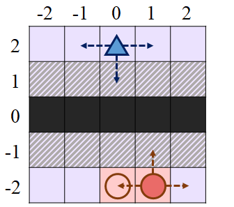
(a) The original grid

(b) The quantized grid

Figure 1: The wall defense problem with the initial conditions $x_{0}^{\text{ag}}=(0,2)$ and $y_{0}=(0,-2)$.

Recall from Subsection III-C that an information state at time $t$ is $\Pi_{t}=\big{(}X_{t}^{\text{ag}},D_{t},[[X_{t}^{\text{at}}|M_{t}]]\big{)}$. We construct an approximation of the conditional range $[[X_{t}^{\text{at}}|M_{t}]]$ at time $t$ using the quantization approach from Subsection IV-D and define the approximate range $\hat{A}_{t}=\big{\{}\mu_{t}(x_{t})\in\hat{\mathcal{X}}^{\text{at}}|x_{t}\in[[X_{t}^{\text{at}}|M_{t}]]\big{\}}$. The set of quantized cells $\hat{\mathcal{X}}^{\text{at}}$, with $\gamma_{t}=1$ for all $t$, is marked in Fig. 1(b) with dots. We consider the approximate information state $\hat{\Pi}_{t}=\big{(}X_{t}^{\text{ag}},D_{t},\hat{A}_{t},Y_{0}\big{)}$ for all $t$. The initial observation $Y_{0}$ in $\hat{\Pi}_{t}$ improves the prediction of $\hat{A}_{t+1}$. For five initial conditions, we compute the best control strategy for $T=6$ using both the information state (IS) and the approximate information state (AIS). In Fig. 2, we present the computational times (Run.) for both the DPs in seconds. Note that the approximate DP has a faster run-time in all cases. We also implement both strategies with random disturbances in the system with $T=6$. In Fig. 2, we also present the actual worst-case costs across $5\times 10^{3}$ implementations of both strategies and note that the AIS has a bounded deviation from the IS.

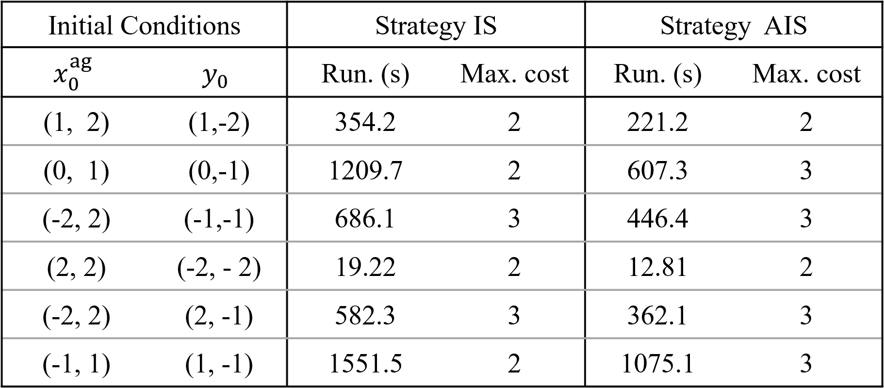
Figure 2: Costs and run-times for $5\times 10^{3}$ simulations and $T=6$.

V-B Pursuit Evasion Problem

In the pursuit evasion problem, we consider an agent who chases a moving target in a $9\times 9$ grid world with static obstacles. The agent aims to get close to the target over a time horizon $T$. For each $t=0,\dots,T$, we denote the position of the agent by $X_{t}^{\text{ag}}\in\mathcal{X}$ and that of the target by $X_{t}^{\text{ta}}\in\mathcal{X}$, where $\mathcal{X}=\big{\{}(-4,-4),\dots,(4,4)\big{\}}\setminus\mathcal{O}$ is the set of feasible grid cells and $\mathcal{O}\subset\mathcal{X}$ is the set of obstacles. The target starts at the position $X_{0}^{\text{ta}}\in\mathcal{X}$, which is updated as $X_{t+1}^{\text{ta}}=\mathbb{I}(X_{t}^{\text{ta}}+W_{t}$ $\in\mathcal{X})\cdot(X_{t}^{\text{ta}}+W_{t})+(1-\mathbb{I}(X_{t}^{\text{ta}}+W_{t}\in\mathcal{X}))\cdot X_{t}^{\text{ta}}$, where $W_{t}\in\mathcal{W}_{t}=\{(-1,0),(1,0),(0,0),(0,1),(0,-1)\}$ is the disturbance. At each $t$, the agent perfectly observes their own position and nosily observes the target’s position as $Y_{t}=\mathbb{I}(X_{t}^{\text{ta}}+N_{t}\in\mathcal{X})\cdot(X_{t}^{\text{ta}}+N_{t})+(1-\mathbb{I}(X_{t}^{\text{ta}}+N_{t}\in\mathcal{X}))$ $\cdot X_{t}^{\text{ta}}$, where $N_{t}\in\mathcal{N}_{t}=\mathcal{W}_{t}$ is the measurement noise. Next, starting with $X_{0}^{\text{ag}}\in\mathcal{X}$, the agent selects an action $U_{t}\in\mathcal{U}_{t}=\mathcal{W}_{t}$ to move as $X_{t+1}^{\text{ag}}=\mathbb{I}(X_{t}^{\text{ag}}+U_{t}\in\mathcal{X})\cdot(X_{t}^{\text{ag}}+U_{t})+(1-\mathbb{I}(X_{t}^{\text{ag}}+U_{t}\in\mathcal{X}))\cdot X_{t}^{\text{ag}}$. At time $T$, the agent selects no action and observes the target’s position $X_{T}^{\text{ta}}$ and incurs a cost $c_{T}(X_{T}^{\text{ta}},X_{T}^{\text{ag}})=\eta(X_{T}^{\text{ta}},X_{T}^{\text{ag}})\in\mathbb{R}_{\geq 0}$, where $\eta$ is the shortest distance between two cells, while avoiding obstacles. The distance between two adjacent cells is $1$ unit. The agent seeks to minimize the worst-case terminal cost without prior knowledge of either the observation function or the target’s evolution dynamics. Note that this is a reinforcement learning generalization of Problem 1. We illustrate the grid and one initial set up in Fig. 3(a). Here, the black cells are obstacles. The solid blue triangle, solid red circle and red ring are the agent, target, and observation, respectively, at $t=0$. The pink cells are feasible positions of the target given the observation.

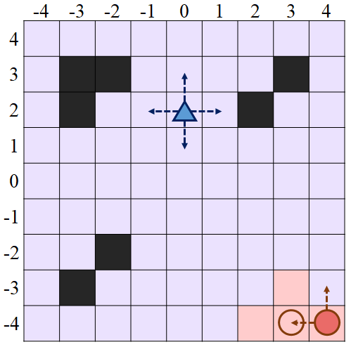
(a) The original problem

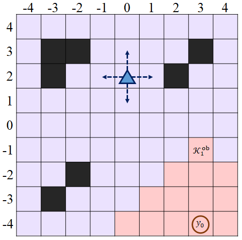
(b) Actual observation prediction

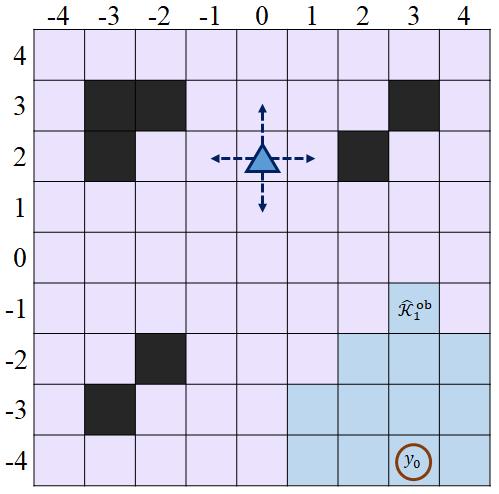
(c) Learned observation prediction

Figure 3: The pursuit evasion problem with the initial conditions $x_{0}^{\text{ag}}=(0,2)$ and $y_{0}=(3,-4)$.

We consider that the agent has access to $3\times 10^{7}$ observation trajectories from the target which are used to learn an approximate information state representation offline, as characterized in Subsection IV-C. First, we use the data on observation trajectories to construct estimates of the conditional range $\mathcal{K}^{\text{ob}}_{t+1}=[[Y_{t+1}|Y_{0:t}]]$ for all $t=0,\dots,T-2$ and $\mathcal{K}^{\text{ob}}_{T}=[[X_{T}^{\text{ta}}|Y_{0:T-1}]]$. Then, taking inspiration from [45], we set-up a deep neural network with an encoder-decoder structure for each $t=0,\dots,T$, as illustrated in Fig. 4. At each $t$, the encoder $\psi_{t}$ comprises of 3 layer neural network with sizes $(2,14)$, $(14,12)$, $(12+24,24)$ and ReLU activation for the first two layers, where the inputs are a $2$-d vector of coordinates for observation $Y_{t}$ and a $24$-d vector for the previous approximate information state $\hat{\Pi}_{t-1}$. The encoder compresses these inputs to a $24$-d vector representing the approximate information state $\hat{\Pi}_{t}$. At each $t$, the decoder $\phi_{t}$ is a 4 layer neural network of size $(24,48)$, $(48,56)$, $(56,64)$, $(64,74)$ with ReLU activation for the first three layers and sigmoid activation for the last layer. Its input is $\hat{\Pi}_{t}$ and its output is a $74$-d vector with each component taking values in $[0,1]$. Each component of the $74$-d output gives a set-inclusion value for a specific feasible cell in the $9\times 9$ grid, excluding obstacles. The output is thus interpreted as the conditional range $\hat{\mathcal{K}}^{\text{ob}}_{t+1}=[[Y_{t+1}~{}|~{}\hat{\Pi}_{t}]]$ for all $t=0,\dots,T-2$ and $\hat{\mathcal{K}}^{\text{ob}}_{T}=[[X_{T}^{\text{ta}}~{}|~{}\hat{\Pi}_{T-1}]]$. We consider a set-inclusion threshold of $0.5$ for inclusion in $\hat{\mathcal{K}}^{\text{ob}}_{t+1}$ at each $t$.

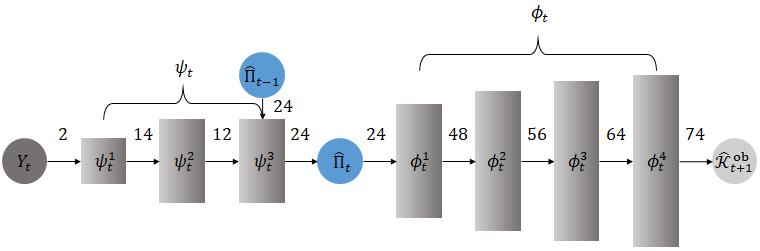
Figure 4: The neural network architecture for approximate information states at any $t=0,\dots,T-1$.

The learning objective of our neural network at each $t$ is to minimize $\mathcal{H}(\mathcal{K}^{\text{ob}}_{t+1},\hat{\mathcal{K}}^{\text{ob}}_{t+1})$, which is consistent with the characterization of approximate information states in Subsection IV-C. Note that at the terminal time step, this objective also minimizes the difference in maximum costs. Since the Hausdorff distance is not differentiable, we adapt the first surrogate function proposed in [92] as a learning objective to train the network weights. We train the network for $40$ epochs using $90\%$ of the available data with a learning rate of $0.0003$ and test it against the other $10\%$. To illustrate the training results, consider an out-of-sample initial observation $y_{0}=(3,-4)$. Then, the set $\mathcal{K}^{\text{ob}}_{1}$ constructed using data is shown by pink cells in 3(b) and the set $\hat{\mathcal{K}}^{\text{ob}}_{1}$ generated by of the trained network is shown by blue cells in 3(c). Note that the trained network’s output matches the conditional range constructed from data accurately except for one cell $(0,-4)$. We train a neural network for each $t$ up to $T=4$ to learn a complete approximate information state representation for the problem. Then, at each $t$, the agent uses the state $(X_{t}^{\text{ag}},\hat{\Pi}_{t})$ in the approximate DP (25) - (26) to compute an approximately optimal control strategy.

We compare the performance of this approximate strategy with a baseline strategy that uses the observation $Y_{t}$ at each $t$ instead of $\hat{\Pi}_{t}$. Thus, for this baseline we train a network to match the prediction $[[Y_{t+1}~{}|~{}Y_{t}]]$ to $[[Y_{t+1}~{}|~{}Y_{0:t}]]$ for all $t=0,\dots,T-2$ and $[[X_{T}^{\text{ta}}~{}|~{}Y_{T-1}]]$ to $[[X_{T}^{\text{ta}}~{}|~{}Y_{0:T-1}]]$ at time $T-1$. The neural network structure is the same as before except for a lack of $\hat{\Pi}_{t-1}$ in the encoder input at each $t$ and we use the same training parameters as before. Subsequently, the agent computes an approximately optimal strategy using the approximate DP with the state $(X_{t}^{\text{ag}},Y_{t})$ at each $t$.

For six initial conditions, we present in Fig. 5 the worst case costs obtained when implementing both the approximately optimal strategy (Maximum cost with AIS) and the baseline strategy (Maximum cost without AIS) for $T=4$. Across $10^{4}$ simulations with randomly generated uncertainties, we note that using the learned approximate information state consistently improves worst-case performance when compared to the baseline. Thus, learning an approximate information state representation is a viable approach for worst-case reinforcement learning. In general, we expect our approach to outperform the baseline more for longer time horizons.

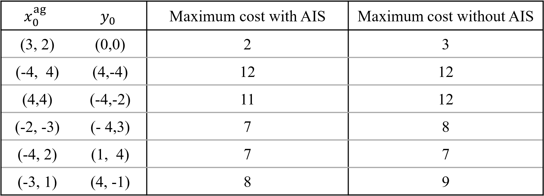
Figure 5: Worst-case costs for $10^{4}$ simulations and $T=4$.

VI Conclusion

In this paper, we presented a principled approach to worst-case control and learning in partially observed systems using non-stochastic approximate information states. We first presented two sets of properties to characterize information states and used them to construct a DP that yields an optimal control strategy. Then, we proposed two sets of properties to characterize approximate information states that can be constructed from output variables with knowledge of the dynamics or learned from output data with incomplete knowledge of the dynamics. We proved that approximate information states can be used in a DP to compute an approximate control strategy with a bounded loss in performance. We also presented theoretical examples of this bound and numerical examples to illustrate the performance of our approach in both worst-case control and reinforcement learning.

Our ongoing work is to specialize the approach in this paper to additive cost problems reported in [93]. Future work should consider extending our results to problems with an infinite time horizon, constructing tighter performance bounds for systems with specific dynamics, and combining these results with other reinforcement learning techniques, e.g., Q-learning [94].

Appendix A – $L$-invertible Functions

In this appendix, we present two classes of functions which are $L$-invertible: 1) all bi-Lipschitz functions which have a compact domain and a compact co-domain, and 2) all functions with a compact domain and a finite co-domain.

Lemma 8.

Let $\mathcal{X}$ and $\mathcal{Y}$ be two compact subsets of a metric space $(\mathcal{S},\eta)$. Then, any bi-Lipischitz function $f:\mathcal{X}\to\mathcal{Y}$ is $L$-invertible.

Proof.

We begin by considering the pre-image set for any $y\in\mathcal{Y}$ under the function $f$. Note that the function $f$ is continuous because it is bi-Lipschitz and the singleton $\{y\}$ is a compact subset of a metric space. Consequently, the pre-image $f^{-1}(y)$ is a bounded subset of $\mathcal{X}$. Next, let $\mathcal{B}(\mathcal{X})$ denote the set of all bounded subsets of $\mathcal{X}$. Given the first result, we can consider a set-valued mapping $f^{-1}:\mathcal{Y}\to\mathcal{B}(\mathcal{X})$ which returns the pre-image for each $y\in\mathcal{Y}$. Then, for any $y^{1},y^{2}\in\mathcal{Y}$, using the definition of the Hausdorff distance in (1):

$$\mathcal{H}\big{(}f^{-1}(y^{1}),f^{-1}(y^{2})\big{)}=\max\Big{\{}\sup_{x^{1}\in f^{-1}(y^{1})}\operatorname*{\vphantom{p}inf}_{x^{2}\in f^{-1}(y^{2})}\\ \eta(x^{1},x^{2}),\sup_{x^{2}\in f^{-1}(y^{2})}\operatorname*{\vphantom{p}inf}_{x^{1}\in f^{-1}(y^{1})}\eta(x^{1},x^{2})\Big{\}}.$$ (61)

In the RHS of (61), the bi-Lipschitz property of $f$ implies that there exist constants $\underline{L}_{f},\overline{L}_{f}\in\mathbb{R}_{>0}$ such that $\underline{L}_{f}\eta(x^{1},x^{2})\leq|f(x^{1})-f(x^{2})|\leq\overline{L}_{f}\eta(x^{1},x^{2}),$ for all $x^{1},x^{2}\in\mathcal{X}$. Thus, for all $x^{1}\in g^{-1}(y^{1})$ and $x^{2}\in g^{-1}(y^{2})$, we write that

$$\eta(x^{1},x^{2})\leq\underline{L}_{f}^{-1}\cdot\eta(y^{1},y^{2}).$$ (62)

The proof is complete by substituting (62) into (61) and defining the constant $L_{f^{-1}}:=\underline{L}_{f}^{-1}$. ∎

Lemma 9.

Let $\mathcal{X}$ be a compact subset and $\mathcal{Y}$ be a finite subset of $(\mathcal{S},\eta)$. Then, any function $f:\mathcal{X}\to\mathcal{Y}$ is $L$-invertible.

Proof.

Let $||\mathcal{Y}||>0$ denote the minimum distance between two distinct elements in the finite, non-empty set $\mathcal{Y}$. Then, for any $y^{1},y^{2}\in\mathcal{Y}$ such that $y^{1}\neq y^{2}$, $\dfrac{\mathcal{H}\big{(}f^{-1}(y^{1}),f^{-1}(y^{2})\big{)}}{\eta(y^{1},y^{2})}$ $\leq\sup_{y^{1},y^{2}\in\mathcal{Y}}\dfrac{\mathcal{H}\big{(}f^{-1}(y^{1}),f^{-1}(y^{2})\big{)}}{||\mathcal{Y}||}=:L_{f^{-1}},$ where $L_{f^{-1}}\in\mathbb{R}_{\geq 0}$ is guaranteed to be finite because the set $\mathcal{X}$ is bounded and thus, so is the numerator. Thus, the function $f$ is $L$-invertible as defined in (61). ∎

Appendix B – Approximation Bounds for Perfectly Observed Systems

In this appendix, we derive the values of $\epsilon_{t}$ and $\delta_{t}$ for all $t=0,\dots,T$ when an approximate information state is constructed using state quantization for a perfectly observed system, as described in Subsection IV-D. We first state a property of the Hausdorff distance which we will use in our derivation.

Lemma 10.

Let $\mathcal{X}$ be a metric space with compact subsets $\mathcal{A},\mathcal{B},\mathcal{C},\mathcal{D}\subset\mathcal{X}$. Then, it holds that

$$\mathcal{H}\big{(}\mathcal{A}\cup\mathcal{B},\mathcal{C}\cup\mathcal{D}\big{)}\leq\max\Big{\{}\mathcal{H}\big{(}\mathcal{A},\mathcal{C}\big{)},\mathcal{H}\big{(}\mathcal{B},\mathcal{D}\big{)}\Big{\}}.$$ (63)

Proof.

The proof for this result is given in [88, Theorem 1.12.15]. ∎

Next, we state and prove the main result of this appendix.

Theorem 5.

Consider a perfectly observed system, i.e., $Y_{t}=X_{t}$, for all $t=0,\dots,T$. Let $\mu_{t}:\mathcal{X}_{t}\to\hat{\mathcal{X}}_{t}$ such that $\max_{x_{t}\in\mathcal{X}_{t}}\eta(x_{t},\mu_{t}(x_{t}))\leq\gamma_{t}$ at each $t$. Then, $\hat{\Pi}_{t}=\mu_{t}(X_{t})$ is an approximate information state which satisfies (22) with $\epsilon_{t}=2L_{d_{t}}\cdot\gamma_{t}$ and (23) with $\delta_{t}=2\gamma_{t+1}+2L_{f_{t}}\cdot\gamma_{t}$ for all $t$, where $\gamma_{T+1}=0$, and where $L_{d_{t}}$, and $L_{f_{t}}$ are Lipschitz constants for $d_{t}$ and $f_{t}$, respectively.

Proof.

For all $t=0,\dots,T$, let $m_{t}=(x_{0:t},u_{0:t-1})$ be the realization of $M_{t}$ and let the approximate information state be $\hat{x}_{t}=\mu_{t}(x_{t})$. We first derive the value of $\epsilon_{t}$ in the RHS of (22). At time $t$, can expand the conditional ranges to write that $[[X_{t}|m_{t}]]=[[X_{t}|x_{t}]]=\{x_{t}\}$ and $[[X_{t}|\hat{x}_{t}]]=\{x_{t}\in\mathcal{X}~{}|~{}\eta(x_{t},\hat{x}_{t})\leq\gamma_{t}\}$. On substituting these into the LHS of (22), we state that $\big{|}\sup_{c_{t}\in[[C_{t}|m_{t},u_{t}]]}c_{t}-\sup_{c_{t}\in[[C_{t}|\mu_{t}(x_{t}),u_{t}]]}c_{t}\big{|}$ $=\big{|}d_{t}(x_{t},u_{t})-\sup_{\bar{x}_{t}\in[[X_{t}|\mu_{t}(x_{t})]]}d_{t}(\bar{x}_{t},u_{t})\big{|}$ $\leq\sup_{\bar{x}_{t}\in[[X_{t}|\mu_{t}(x_{t})]]}|d_{t}(x_{t},u_{t})-d_{t}(\bar{x}_{t},u_{t})|$ $\leq L_{d_{t}}\cdot\sup_{\bar{x}_{t}\in[[X_{t}|\mu_{t}(x_{t})]]}\eta(x_{t},\bar{x}_{t})$ $\leq L_{d_{t}}\cdot\big{(}\eta(x_{t},\mu_{t}(x_{t}))+\sup_{\bar{x}_{t}\in[[X_{t}|\mu_{t}(x_{t})]]}\eta(\mu_{t}(x_{t}),\bar{x}_{t})\big{)},$ $\leq 2L_{d_{t}}\cdot\gamma_{t}=:\epsilon_{t}$, where, in the third inequality, we use the triangle inequality. Next, to derive the value of $\delta_{t}$, we expand the LHS of (23) as

$$\mathcal{H}\big{(}[[\hat{X}_{t+1}|x_{t},u_{t}]],[[\hat{X}_{t+1}|\mu_{t}(x_{t}),u_{t}]]\big{)}$$

$$= \mathcal{H}\big{(}\big{\{}\mu_{t+1}(f_{t}(x_{t},u_{t},w_{t}))|w_{t}\in\mathcal{W}_{t}\big{\}},$$

$$\big{\{}\mu_{t+1}(f_{t}(\bar{x}_{t},u_{t},w_{t}))|\bar{x}_{t}\in[[X_{t}|\mu_{t}(x_{t})]],w_{t}\in\mathcal{W}_{t}\big{\}}\big{)}$$

$$\leq \sup_{w_{t}\in\mathcal{W}_{t}}\mathcal{H}(\{\mu_{t+1}(f_{t}(x_{t},u_{t},w_{t}))\},$$

$$\{\mu_{t+1}(f_{t}(\bar{x}_{t},u_{t},w_{t}))|\bar{x}_{t}\in[[X_{t}|\mu_{t}(x_{t})]]\}),$$ (64)

where, in the inequality, we use (63) from Lemma 10 and the fact that $\big{\{}\mu_{t+1}(f_{t}(x_{t},u_{t},w_{t}))|w_{t}\in\mathcal{W}_{t}\big{\}}=\cup_{w_{t}\in\mathcal{W}_{t}}\big{\{}\mu_{t+1}(f_{t}(\bar{x}_{t},u_{t},w_{t}))\big{\}}$. Once again using (63) in the RHS of (64), we conclude that $\mathcal{H}\big{(}[[\hat{X}_{t+1}|x_{t},u_{t}]],[[\hat{X}_{t+1}|\mu_{t}(x_{t}),u_{t}]]\big{)}\leq\sup_{w_{t}\in\mathcal{W}_{t},\bar{x}_{t}\in[[X_{t}|\mu_{t}(x_{t})]]}\eta\big{(}\mu_{t+1}\big{(}f_{t}(x_{t},u_{t},w_{t})\big{)},\mu_{t+1}\big{(}f_{t}(\bar{x}_{t},$ $u_{t},w_{t})\big{)}\big{)}$ $\leq\sup_{w_{t}\in\mathcal{W}_{t},\bar{x}_{t}\in[[X_{t}|\mu_{t}(x_{t})]]}\big{(}\eta\big{(}\mu_{t+1}(f_{t}(x_{t},u_{t},w_{t})),$ $f_{t}(x_{t},u_{t},w_{t})\big{)}+\eta\big{(}f_{t}(x_{t},u_{t},w_{t}),f_{t}(\bar{x}_{t},u_{t},w_{t})\big{)}+$ $\eta\big{(}f_{t}(\bar{x}_{t},u_{t},w_{t}),\mu_{t+1}(f_{t}(\bar{x}_{t},u_{t},w_{t}))\big{)}\big{)}\leq\gamma_{t+1}+2L_{f_{t}}\cdot\gamma_{t}+\gamma_{t+1}=:\delta_{t},$ where, in the second inequality, we use the triangle inequality. ∎

Appendix C – Approximation Bounds for Partially Observed Systems

In this appendix, we derive the values of $\epsilon_{t}$ and $\delta_{t}$ for all $t=0,\dots,T$, when an approximate information state is constructed using state quantization for a partially observed system, as described in Subsection IV-D.

Theorem 6.

Consider a partially observed system with $Y_{t}=h_{t}(X_{t},N_{t})$ for all $t=0,\dots,T$. Let $\mu_{t}:\mathcal{X}_{t}\to\hat{\mathcal{X}}_{t}$ such that $\sup_{x_{t}\in\mathcal{X}_{t}}\eta(x_{t},\mu_{t}(x_{t}))\leq\gamma_{t}$ at each $t$. Then, $\hat{\Pi}_{t}=\nu_{t}(\Pi_{t})$ is an approximate information state with $\epsilon_{t}=2L_{d_{t}}\cdot\gamma_{t}$ and $\delta_{t}=2\gamma_{t+1}+2L_{\bar{f}_{t}}\cdot L_{h_{t+1}}\cdot L_{f_{t}}\cdot\gamma_{t}$ for all $t$, where $\gamma_{T+1}=0$, and where $L_{d_{t}}$, $L_{\bar{f}_{t}}$, $L_{h_{t+1}}$, and $L_{f_{t}}$ are Lipschitz constants for the respective functions in the subscripts.

Proof.

For all $t=0,\dots,T$, let $m_{t}\in[[M_{t}]]$, $P_{t}=[[X_{t}|m_{t}]]\in\mathcal{P}_{t}$, and $\hat{P}_{t}=\nu_{t}(P_{t})\in\hat{\mathcal{P}}_{t}$ be the realizations of the memory $M_{t}$, the conditional range $\Pi_{t}$ and the approximate information state $\hat{\Pi}_{t}$, respectively. Note that the conditional range $P_{t}$ satisfies (14) and (15) from Definition 3. Next, to derive the value of $\epsilon_{t}$, we write the LHS of (22) using (14) as

$$\big{|}\sup_{c_{t}\in[[C_{t}|m_{t},u_{t}]]}c_{t}-\sup_{c_{t}\in[[C_{t}|\nu_{t}({P}_{t}),u_{t}]]}c_{t}\big{|}$$

$$= \big{|}\sup_{x_{t}\in P_{t}}d_{t}(x_{t},u_{t})-\sup_{\bar{x}_{t}\in[[X_{t}|\nu_{t}({P}_{t})]])}d_{t}(\bar{x}_{t},u_{t})\big{|}$$

$$\leq L_{d_{t}}\cdot\mathcal{H}(P_{t},[[X_{t}|\nu_{t}({P}_{t})]])$$

$$\leq L_{d_{t}}\cdot\big{(}\mathcal{H}(P_{t},\nu_{t}(P_{t}))+\mathcal{H}(\nu_{t}(P_{t}),[[X_{t}|\nu_{t}({P}_{t})]])\big{)},$$ (65)

where, in the equality, we use (14); in the first inequality, we use (34) from Lemma 5; and in the second inequality we use the triangle inequality for the Hausdorff distance. We can expand the first term in the RHS of (65) as $\mathcal{H}(P_{t},\nu_{t}(P_{t}))=\mathcal{H}(P_{t},\{\mu_{t}(x_{t})\in\hat{\mathcal{X}}_{t}\;|\;x_{t}\in P_{t}\})$ $=\mathcal{H}\big{(}\cup_{x_{t}\in P_{t}}\{x_{t}\},\cup_{x_{t}\in P_{t}}\{\mu_{t}(x_{t})\in\hat{\mathcal{X}}_{t}\}\big{)}\leq\sup_{x_{t}\in P_{t}}$ $\eta(x_{t},\mu_{t}(x_{t}))\leq\gamma_{t}$, where we use (63) from Lemma 10 in the first inequality. We can also expand the second term in the RHS of (65) as $\mathcal{H}(\nu_{t}(P_{t}),[[X_{t}|\nu_{t}({P}_{t})]]))=\mathcal{H}\big{(}\nu_{t}(P_{t}),\{x_{t}\in\mathcal{X}_{t}|\operatorname*{\vphantom{p}inf}_{\bar{x}_{t}\in\nu_{t}(P_{t})}\eta(x_{t},\bar{x}_{t})\leq\gamma_{t}\}\big{)}=\sup_{x_{t}\in[[X_{t}|\nu_{t}(P_{t})]]}\operatorname*{\vphantom{p}inf}_{\bar{x}_{t}\in\nu_{t}(P_{t})}\eta(x_{t},\bar{x}_{t})\leq\gamma_{t}$, where the second equality holds by expanding the Hausdorff distance and noting that $\nu_{t}(P_{t})\subseteq[[X_{t}|\nu_{t}(P_{t})]]$. The proof is complete by substituting the results for both terms in the RHS of (65).

Next, to derive the value of $\delta_{t}$, we note that $P_{t}=\sigma_{t}(m_{t})$. Then, using the triangle inequality in the LHS of (23),

$$\mathcal{H}\big{(}[[\nu_{t+1}(\Pi_{t+1})|m_{t},u_{t}]],[[\nu_{t+1}(\Pi_{t+1})|\nu_{t}(\sigma_{t}(m_{t})),u_{t}]]\big{)}$$

$$\leq \mathcal{H}\big{(}[[\nu_{t+1}(\Pi_{t+1})|m_{t},u_{t}]],[[\Pi_{t+1}|m_{t},u_{t}]]\big{)}+$$

$$\mathcal{H}\big{(}[[\Pi_{t+1}|m_{t},u_{t}]],[[\Pi_{t+1}|\nu_{t}(\sigma_{t}(m_{t})),u_{t}]]\big{)}+$$

$$\mathcal{H}\big{(}[[\Pi_{t+1}|\nu_{t}(\sigma_{t}(m_{t})),u_{t}]],[[\nu_{t+1}(\Pi_{t+1})|\nu_{t}(\sigma_{t}(m_{t})),u_{t}]]\big{)}$$

$$\leq 2\gamma_{t+1}+\mathcal{H}\big{(}[[\Pi_{t+1}|m_{t},u_{t}]],[[\Pi_{t+1}|\nu_{t}(\sigma_{t}(m_{t})),u_{t}]]\big{)},$$ (66)

where, in the second inequality we use the fact that $\mathcal{H}\big{(}P_{t+1},\nu_{t+1}(P_{t+1})\big{)}\leq\gamma_{t+1}$, which was proved above. We can write the second term in the RHS of (66) using (15) from Definition 3 as $\mathcal{H}\big{(}[[\Pi_{t+1}|m_{t},u_{t}]],[[\Pi_{t+1}|\nu_{t}(\sigma_{t}(m_{t})),u_{t}]]\big{)}=\mathcal{H}\big{(}[[\Pi_{t+1}|P_{t},u_{t}]],[[\Pi_{t+1}|\nu_{t}(P_{t}),u_{t}]]\big{)}$. Furthermore, note that $[[\Pi_{t+1}|\nu_{t}(P_{t}),u_{t}]]=\big{\{}\tilde{P}_{t+1}\in[[\Pi_{t+1}|\tilde{P}_{t},u_{t}]]$ $|\tilde{P}_{t}\in[[\Pi_{t}|\nu_{t}(P_{t})]]\big{\}}=\cup_{\tilde{P}_{t}\in[[\Pi_{t}|\nu(P_{t})]]}[[\Pi_{t+1}|\tilde{P}_{t},u_{t}]]$. Next, we use (63) from Lemma 10 to write that

$$\mathcal{H}\big{(}[[\Pi_{t+1}|P_{t},u_{t}]]),[[\Pi_{t+1}|\nu_{t}(P_{t}),u_{t}]]\big{)}$$

$$\leq \sup_{\tilde{P}_{t}\in[[\Pi_{t}|\nu_{t}(P_{t})]]}\mathcal{H}\big{(}[[\Pi_{t+1}|P_{t},u_{t}]]),[[\Pi_{t+1}|\tilde{P}_{t},u_{t}]]\big{)}$$

$$\leq L_{\bar{f}_{t}}\cdot\sup_{\tilde{P}_{t}\in[[\Pi_{t}|\nu_{t}(P_{t})]]}\mathcal{H}\big{(}[[Y_{t+1}|P_{t},u_{t}]]),[[Y_{t+1}|\tilde{P}_{t},u_{t}]]\big{)}$$

$$\leq L_{\bar{f}_{t}}\cdot L_{h_{t+1}}\cdot\sup_{\tilde{P}_{t}\in[[\Pi_{t}|\nu_{t}(P_{t})]]}\mathcal{H}\big{(}[[X_{t+1}|P_{t},u_{t}]]),[[X_{t+1}|\tilde{P}_{t},u_{t}]]\big{)},$$ (67)

where, in the second inequality we use the same arguments as in Lemma 6 and the third inequality can be proven by substituting $Y_{t+1}=h_{t+1}(X_{t+1},V_{t+1})$ into the equation. We can further expand the third term in the RHS of (67) and use (63) from Lemma (10) to write that $\sup_{\tilde{P}_{t}\in[[\Pi_{t}|\nu_{t}(P_{t})]]}\mathcal{H}\big{(}[[X_{t+1}|P_{t},u_{t}]]),[[X_{t+1}|\tilde{P}_{t},u_{t}]]\big{)}$ $\leq\sup_{\tilde{P}_{t}\in[[\Pi_{t}|\nu_{t}(P_{t})]],w_{t}\in\mathcal{W}_{t}}\mathcal{H}\big{(}\{f_{t}(x_{t},u_{t},w_{t})|x_{t}\in P_{t}\},$ $\{f_{t}(x_{t},u_{t},w_{t})|x_{t}\in\tilde{P}_{t}\}\big{)}$ $\leq L_{f_{t}}\cdot\sup_{\tilde{P}_{t}\in[[\Pi_{t}|\nu_{t}(P_{t})]]}\mathcal{H}\big{(}P_{t},\tilde{P}_{t}\big{)}$ $\leq L_{f_{t}}\cdot\sup_{\tilde{P}_{t}\in[[\Pi_{t}|\nu_{t}(P_{t})]]}\big{(}\mathcal{H}(P_{t},\nu_{t}(P_{t})\big{)}+\mathcal{H}\big{(}\nu_{t}(P_{t}),\tilde{P}_{t})\big{)}$ $\leq 2L_{f_{t}}\cdot\gamma_{t},$ where, in the third inequality, we use the triangle inequality and in the fourth inequality we use the fact that for all $\nu_{t}(\tilde{P}_{t})=\nu_{t}(P_{t})$, for all $\tilde{P}_{t}\in[[\Pi_{t}|\nu_{t}(P_{t})]]$. ∎

Aditya Dave (S’18) is a PhD candidate in the Department of Mechanical Engineering at the University of Delaware, Newark, USA since 2017. He received a B. Tech. in Mechanical Engineering from the Indian Institute of Technology, Bombay, India, in 2016. Prior to his PhD degree, he worked as a Project Manager at Cairn Energy, Gurugram, India from 2016-2017. His current research interests span several areas, including worst-case control, reinforcement learning, decentralized systems, and mechanism design. He is a student member of IEEE.

Nishanth Venkatesh S (S’21) is research engineer at the Department of Mechanical Engineering at the University of Delaware, Newark, USA. He received a Master’s degree in Robotics from the University of Delaware, Newark, USA, 2021. Prior to his Master’s he received a B. Tech. in Mechanical Engineering from the Indian Institute of Technology, Bombay, India, in 2019. His current research interests span several areas, including worst-case control, reinforcement learning, and decentralized systems. He is a student member of IEEE.

Andreas A. Malikopoulos (S’06–M’09–SM’17) received the Diploma in mechanical engineering from the National Technical University of Athens, Greece, in 2000. He received M.S. and Ph.D. degrees from the department of mechanical engineering at the University of Michigan, Ann Arbor, Michigan, USA, in 2004 and 2008, respectively. He is the Terri Connor Kelly and John Kelly Career Development Associate Professor in the Department of Mechanical Engineering at the University of Delaware, the Director of the Information and Decision Science (IDS) Laboratory, and the Director of the Sociotechnical Systems Center. Prior to these appointments, he was the Deputy Director and the Lead of the Sustainable Mobility Theme of the Urban Dynamics Institute at Oak Ridge National Laboratory, and a Senior Researcher with General Motors Global Research & Development. His research spans several fields, including analysis, optimization, and control of cyber-physical systems; decentralized systems; stochastic scheduling and resource allocation problems; and learning in complex systems. The emphasis is on applications related to smart cities, emerging mobility systems, and sociotechnical systems. He has been an Associate Editor of the IEEE Transactions on Intelligent Vehicles and IEEE Transactions on Intelligent Transportation Systems from 2017 through 2020. He is currently an Associate Editor of Automatica and IEEE Transactions on Automatic Control. He is a member of SIAM, AAAS, and a Fellow of the ASME.

References

- [1] K.-D. Kim and P. R. Kumar, “Cyber–physical systems: A perspective at the centennial,” Proceedings of the IEEE, vol. 100, no. Special Centennial Issue, pp. 1287–1308, 2012.
- [2] A. A. Malikopoulos, L. E. Beaver, and I. V. Chremos, “Optimal time trajectory and coordination for connected and automated vehicles,” Automatica, vol. 125, no. 109469, 2021.
- [3] A. Dave, I. V. Chremos, and A. A. Malikopoulos, “Social media and misleading information in a democracy: A mechanism design approach,” IEEE Transactions on Automatic Control, vol. 67, no. 5, pp. 2633–2639, 2022.
- [4] L. E. Beaver and A. A. Malikopoulos, “An Overview on Optimal Flocking,” Annual Reviews in Control, vol. 51, pp. 88–99, 2021.
- [5] P. R. Kumar and P. P. Varaiya, Stochastic Systems: Estimation, Identification, and Adaptive Control. Englewood Cliffs, NJ: Prentice-Hall, 1986.
- [6] N. Bäauerle and U. Rieder, “Partially observable risk-sensitive markov decision processes,” Mathematics of Operations Research, vol. 42, no. 4, pp. 1180–1196, 2017.
- [7] A. A. Malikopoulos, “A duality framework for stochastic optimal control of complex systems,” IEEE Transactions on Automatic Control, vol. 61, no. 10, pp. 2756–2765, 2016.
- [8] M. Ahmadi, N. Jansen, B. Wu, and U. Topcu, “Control theory meets pomdps: A hybrid systems approach,” IEEE Transactions on Automatic Control, vol. 66, no. 11, pp. 5191–5204, 2020.
- [9] A. Mahajan, N. C. Martins, M. C. Rotkowitz, and S. Yüksel, “Information structures in optimal decentralized control,” in 2012 IEEE 51st IEEE Conference on Decision and Control (CDC), pp. 1291–1306, IEEE, 2012.
- [10] A. Dave and A. A. Malikopoulos, “Decentralized stochastic control in partially nested information structures,” IFAC-PapersOnLine, vol. 52, no. 20, pp. 97–102, 2019.
- [11] A. Dave and A. A. Malikopoulos, “A dynamic program for a team of two agents with nested information,” in 2021 IEEE Conference on Decision and Control (CDC), pp. 3768–3773, IEEE, 2021.
- [12] A. Dave, N. Venkatesh, and A. A. Malikopoulos, “On decentralized control of two agents with nested accessible information,” in 2022 American Control Conference (ACC), pp. 3423–3430, IEEE, 2022.
- [13] A. A. Malikopoulos, “On team decision problems with nonclassical information structures,” IEEE Transactions on Automatic Control, 2023.
- [14] R. S. Sutton and A. G. Barto, Reinforcement learning: An introduction. MIT press, 2018.
- [15] R. K. Mishra, D. Vasal, and S. Vishwanath, “Decentralized multi-agent reinforcement learning with shared actions,” in 2021 55th Annual Conference on Information Sciences and Systems (CISS), pp. 1–6, IEEE, 2021.
- [16] K. Zhang, Z. Yang, and T. Başar, “Multi-agent reinforcement learning: A selective overview of theories and algorithms,” Handbook of Reinforcement Learning and Control, pp. 321–384, 2021.
- [17] H. Kao and V. Subramanian, “Common information based approximate state representations in multi-agent reinforcement learning,” in International Conference on Artificial Intelligence and Statistics, pp. 6947–6967, PMLR, 2022.
- [18] A. A. Malikopoulos, “Separation of learning and control for cyber-physical systems,” Automatica, 2023 (in press).
- [19] S. Mannor, D. Simester, P. Sun, and J. N. Tsitsiklis, “Bias and variance approximation in value function estimates,” Management Science, vol. 53, no. 2, pp. 308–322, 2007.
- [20] L. Brunke, M. Greeff, A. W. Hall, Z. Yuan, S. Zhou, J. Panerati, and A. P. Schoellig, “Safe learning in robotics: From learning-based control to safe reinforcement learning,” Annual Review of Control, Robotics, and Autonomous Systems, vol. 5, pp. 411–444, 2022.
- [21] T. Başar and P. Bernhard, H-infinity optimal control and related minimax design problems: a dynamic game approach. Springer Science & Business Media, 2008.
- [22] M. Rasouli, E. Miehling, and D. Teneketzis, “A scalable decomposition method for the dynamic defense of cyber networks,” in Game Theory for Security and Risk Management, pp. 75–98, Springer, 2018.
- [23] Y. Shoukry, J. Araujo, P. Tabuada, M. Srivastava, and K. H. Johansson, “Minimax control for cyber-physical systems under network packet scheduling attacks,” in Proceedings of the 2nd ACM international conference on High confidence networked systems, pp. 93–100, 2013.
- [24] M. Giuliani, J. Lamontagne, P. Reed, and A. Castelletti, “A state-of-the-art review of optimal reservoir control for managing conflicting demands in a changing world,” Water Resources Research, vol. 57, no. 12, p. e2021WR029927, 2021.
- [25] Q. Zhu and T. Başar, “Robust and resilient control design for cyber-physical systems with an application to power systems,” in 2011 50th IEEE Conference on Decision and Control and European Control Conference, pp. 4066–4071, IEEE, 2011.
- [26] K. J. Åström and P. R. Kumar, “Control: A perspective.,” Autom., vol. 50, no. 1, pp. 3–43, 2014.
- [27] V.-A. Le and A. A. Malikopoulos, “A Cooperative Optimal Control Framework for Connected and Automated Vehicles in Mixed Traffic Using Social Value Orientation,” in 2022 61th IEEE Conference on Decision and Control (CDC), pp. 6272–6277, 2022.
- [28] D. Hadfield-Menell, S. J. Russell, P. Abbeel, and A. Dragan, “Cooperative inverse reinforcement learning,” Advances in neural information processing systems, vol. 29, 2016.
- [29] M. Fatemi, T. W. Killian, J. Subramanian, and M. Ghassemi, “Medical dead-ends and learning to identify high-risk states and treatments,” Advances in Neural Information Processing Systems, vol. 34, pp. 4856–4870, 2021.
- [30] B. Kiumarsi, K. G. Vamvoudakis, H. Modares, and F. L. Lewis, “Optimal and autonomous control using reinforcement learning: A survey,” IEEE transactions on neural networks and learning systems, vol. 29, no. 6, pp. 2042–2062, 2017.
- [31] B. Recht, “A tour of reinforcement learning: The view from continuous control,” Annual Review of Control, Robotics, and Autonomous Systems, vol. 2, pp. 253–279, 2019.
- [32] D. Bertsekas and J. N. Tsitsiklis, Neuro-dynamic programming. Athena Scientific, 1996.
- [33] D. P. Bertsekas, “Dynamic programming and suboptimal control: A survey from adp to mpc,” European Journal of Control, vol. 11, no. 4-5, pp. 310–334, 2005.
- [34] W. B. Powell, Approximate Dynamic Programming: Solving the curses of dimensionality, vol. 703. John Wiley & Sons, 2007.
- [35] D. P. Bertsekas, Control of uncertain systems with a set-membership description of the uncertainty. PhD thesis, Massachusetts Institute of Technology, 1971.
- [36] D. Bertsekas, “Distributed asynchronous policy iteration for sequential zero-sum games and minimax control,” arXiv preprint arXiv:2107.10406, 2021.
- [37] O. Hernández-Lerma and J. B. Lasserre, Discrete-time Markov control processes: basic optimality criteria, vol. 30. Springer Science & Business Media, 2012.
- [38] J. Moon and T. Başar, “Minimax control over unreliable communication channels,” Automatica, vol. 59, pp. 182–193, 2015.
- [39] D. Bertsekas, Dynamic programming and optimal control: Volume I, vol. 1. Athena scientific, 2012.
- [40] C. H. Papadimitriou and J. N. Tsitsiklis, “The complexity of markov decision processes,” Mathematics of operations research, vol. 12, no. 3, pp. 441–450, 1987.
- [41] P. Bernhard, “A separation theorem for expected value and feared value discrete time control,” ESAIM: Control, Optimisation and Calculus of Variations, vol. 1, pp. 191–206, 1996.
- [42] M. L. Puterman, Markov decision processes: discrete stochastic dynamic programming. John Wiley & Sons, 2014.
- [43] A. Nayyar, A. Mahajan, and D. Teneketzis, “Decentralized stochastic control with partial history sharing: A common information approach,” IEEE Transactions on Automatic Control, vol. 58, no. 7, pp. 1644–1658, 2013.
- [44] A. Dave and A. A. Malikopoulos, “Structural results for decentralized stochastic control with a word-of-mouth communication,” in 2020 American Control Conference (ACC), pp. 2796–2801, IEEE, 2020.
- [45] J. Subramanian and A. Mahajan, “Approximate information state for partially observed systems,” in 2019 IEEE 58th Conference on Decision and Control (CDC), pp. 1629–1636, IEEE, 2019.
- [46] Y. Cong, X. Wang, and X. Zhou, “Rethinking the mathematical framework and optimality of set-membership filtering,” IEEE Transactions on Automatic Control, vol. 67, no. 5, pp. 2544–2551, 2021.
- [47] D. P. Bertsekas and I. B. Rhodes, “On the minimax reachability of target sets and target tubes,” Automatica, vol. 7, no. 2, pp. 233–247, 1971.
- [48] D. Bertsekas and I. Rhodes, “Sufficiently informative functions and the minimax feedback control of uncertain dynamic systems,” IEEE Transactions on Automatic Control, vol. 18, no. 2, pp. 117–124, 1973.
- [49] M. Gagrani and A. Nayyar, “Decentralized minimax control problems with partial history sharing,” in 2017 American Control Conference (ACC), pp. 3373–3379, IEEE, 2017.
- [50] A. Dave, N. Venkatesh, and A. A. Malikopoulos, “On decentralized minimax control with nested subsystems,” in 2022 American Control Conference (ACC), pp. 3437–3444, IEEE, 2022.
- [51] R. R. Moitié, M. Quincampoix, and V. M. Veliov, “Optimal control of discrete-time uncertain systems with imperfect measurement,” IEEE transactions on automatic control, vol. 47, no. 11, pp. 1909–1914, 2002.
- [52] C. Piccardi, “Infinite-horizon minimax control with pointwise cost functional,” Journal of Optimization Theory and Applications, vol. 78, no. 2, pp. 317–336, 1993.
- [53] P. Bernhard, “Minimax - or feared value - / control,” Theoretical computer science, vol. 293, no. 1, pp. 25–44, 2003.
- [54] M. Gagrani, Y. Ouyang, M. Rasouli, and A. Nayyar, “Worst-case guarantees for remote estimation of an uncertain source,” IEEE Transactions on Automatic Control, vol. 66, no. 4, pp. 1794–1801, 2020.
- [55] M. R. James, J. S. Baras, and R. J. Elliott, “Risk-sensitive control and dynamic games for partially observed discrete-time nonlinear systems,” IEEE transactions on automatic control, vol. 39, no. 4, pp. 780–792, 1994.
- [56] P. Bernhard, “Max-plus algebra and mathematical fear in dynamic optimization,” Set-Valued Analysis, vol. 8, no. 1, pp. 71–84, 2000.
- [57] J. S. Baras and N. S. Patel, “Robust control of set-valued discrete-time dynamical systems,” IEEE Transactions on Automatic Control, vol. 43, no. 1, pp. 61–75, 1998.
- [58] S. P. Coraluppi and S. I. Marcus, “Risk-sensitive and minimax control of discrete-time, finite-state markov decision processes,” Automatica, vol. 35, no. 2, pp. 301–309, 1999.
- [59] A. Dave, N. Venkatesh, and A. A. Malikopoulos, “Approximate information states for worst-case control of uncertain systems,” in Proceedings of the 61th IEEE Conference on Decision and Control (CDC), pp. 4945–4950, 2022.
- [60] S. P. Coraluppi and S. I. Marcus, “Mixed risk-neutral/minimax control of discrete-time, finite-state markov decision processes,” IEEE Transactions on Automatic Control, vol. 45, no. 3, pp. 528–532, 2000.
- [61] G. N. Iyengar, “Robust dynamic programming,” Mathematics of Operations Research, vol. 30, no. 2, pp. 257–280, 2005.
- [62] T. Osogami, “Robust partially observable markov decision process,” in International Conference on Machine Learning, pp. 106–115, PMLR, 2015.
- [63] E. Gallestey, M. James, and W. McEneaney, “Max-plus methods in partially observed h/sub/spl infin//control,” in Proceedings of the 38th IEEE Conference on Decision and Control (Cat. No. 99CH36304), vol. 3, pp. 3011–3016, IEEE, 1999.
- [64] N. Saldi, T. Linder, and S. Yüksel, “Asymptotic optimality and rates of convergence of quantized stationary policies in stochastic control,” IEEE Transactions on Automatic Control, vol. 60, no. 2, pp. 553–558, 2014.
- [65] S. Meyn, Control Systems and Reinforcement Learning. Cambridge University Press, 2022.
- [66] S. Levine, A. Kumar, G. Tucker, and J. Fu, “Offline reinforcement learning: Tutorial, review, and perspectives on open problems,” arXiv preprint arXiv:2005.01643, 2020.
- [67] A. A. Malikopoulos, P. Y. Papalambros, and D. N. Assanis, “A Real-Time Computational Learning Model for Sequential Decision-Making Problems Under Uncertainty,” Journal of Dynamic Systems, Measurement, and Control, vol. 131, 05 2009. 041010.
- [68] T. M. Moerland, J. Broekens, and C. M. Jonker, “Model-based reinforcement learning: A survey,” arXiv preprint arXiv:2006.16712, 2020.
- [69] J. Ramírez, W. Yu, and A. Perrusquía, “Model-free reinforcement learning from expert demonstrations: a survey,” Artificial Intelligence Review, vol. 55, no. 4, pp. 3213–3241, 2022.
- [70] J. Morimoto and K. Doya, “Robust reinforcement learning,” Neural computation, vol. 17, no. 2, pp. 335–359, 2005.
- [71] M. Heger, “Consideration of risk in reinforcement learning,” in Machine Learning Proceedings 1994, pp. 105–111, Elsevier, 1994.
- [72] G. Jiang, C.-P. Wu, and G. Cybenko, “Minimax-based reinforcement learning with state aggregation,” in Proceedings of the 37th IEEE Conference on Decision and Control (Cat. No. 98CH36171), vol. 2, pp. 1236–1241, IEEE, 1998.
- [73] A. Al-Tamimi, F. L. Lewis, and M. Abu-Khalaf, “Model-free q-learning designs for linear discrete-time zero-sum games with application to h-infinity control,” Automatica, vol. 43, no. 3, pp. 473–481, 2007.
- [74] J. Garcıa and F. Fernández, “A comprehensive survey on safe reinforcement learning,” Journal of Machine Learning Research, vol. 16, no. 1, pp. 1437–1480, 2015.
- [75] A. P. Valadbeigi, A. K. Sedigh, and F. L. Lewis, “H∞ static output-feedback control design for discrete-time systems using reinforcement learning,” IEEE transactions on neural networks and learning systems, vol. 31, no. 2, pp. 396–406, 2019.
- [76] S. Chakravorty and D. Hyland, “Minimax reinforcement learning,” in AIAA Guidance, Navigation, and Control Conference and Exhibit, p. 5718, 2003.
- [77] B. Kiumarsi, F. L. Lewis, and Z.-P. Jiang, “H∞ control of linear discrete-time systems: Off-policy reinforcement learning,” Automatica, vol. 78, pp. 144–152, 2017.
- [78] N. Agarwal, B. Bullins, E. Hazan, S. Kakade, and K. Singh, “Online control with adversarial disturbances,” in International Conference on Machine Learning, pp. 111–119, PMLR, 2019.
- [79] P. Gradu, J. Hallman, and E. Hazan, “Non-stochastic control with bandit feedback,” Advances in Neural Information Processing Systems, vol. 33, pp. 10764–10774, 2020.
- [80] M. Littman and R. S. Sutton, “Predictive representations of state,” Advances in neural information processing systems, vol. 14, 2001.
- [81] J. Subramanian, A. Sinha, R. Seraj, and A. Mahajan, “Approximate information state for approximate planning and reinforcement learning in partially observed systems,” Journal of Machine Learning Research, vol. 23, no. 12, pp. 1–83, 2022.
- [82] G. Patil, A. Mahajan, and D. Precup, “On learning history based policies for controlling markov decision processes,” arXiv preprint arXiv:2211.03011, 2022.
- [83] A. D. Kara and S. Yüksel, “Near optimality of finite memory feedback policies in partially observed markov decision processes.,” Journal of Machine Learning Research, vol. 23, pp. 11–1, 2022.
- [84] L. Yang, K. Zhang, A. Amice, Y. Li, and R. Tedrake, “Discrete approximate information states in partially observable environments,” in 2022 American Control Conference (ACC), pp. 1406–1413, IEEE, 2022.
- [85] T. W. Killian, H. Zhang, J. Subramanian, M. Fatemi, and M. Ghassemi, “An empirical study of representation learning for reinforcement learning in healthcare,” in Machine Learning for Health, pp. 139–160, PMLR, 2020.
- [86] G. N. Nair, “A nonstochastic information theory for communication and state estimation,” IEEE Transactions on automatic control, vol. 58, no. 6, pp. 1497–1510, 2013.
- [87] A. Girard and G. J. Pappas, “Approximation metrics for discrete and continuous systems,” IEEE Transactions on Automatic Control, vol. 52, no. 5, pp. 782–798, 2007.
- [88] M. F. Barnsley, Superfractals. Cambridge University Press, 2006.
- [89] G. Didinsky, Design of minimax controllers for nonlinear systems using cost-to-come methods. University of Illinois at Urbana-Champaign, 1995.
- [90] P. Bernhard, Sketch of a theory of nonlinear partial information min-max control. PhD thesis, INRIA, 1993.
- [91] D. Bertsekas, “Convergence of discretization procedures in dynamic programming,” IEEE Transactions on Automatic Control, vol. 20, no. 3, pp. 415–419, 1975.
- [92] D. Karimi and S. E. Salcudean, “Reducing the hausdorff distance in medical image segmentation with convolutional neural networks,” IEEE Transactions on medical imaging, vol. 39, no. 2, pp. 499–513, 2019.
- [93] A. Dave, N. Venkatesh, and A. A. Malikopoulos, “On non-stochastic approximate information states for uncertain systems with additive costs,” arXiv preprint, arXiv:2209.13787, 2022.
- [94] A. D. Kara and S. Yüksel, “Convergence and near optimality of q-learning with finite memory for partially observed models,” in 2021 60th IEEE Conference on Decision and Control (CDC), pp. 1603–1608, IEEE, 2021.