Extreme mass ratio inspirals in galaxies with dark matter halos

Abstract

Using the analytic, static and spherically symmetric metric for a Schwarzschild black hole immersed in dark matter (DM) halos with Hernquist type density distribution, we derive analytic formulae for the orbital period and orbital precession, the evolutions of the semi-latus rectum and the eccentricity for eccentric EMRIs with the environment of DM halos. We show how orbital precessions are decreased and even reverse the direction if the density of DM halo is large enough. The presence of local DM halos slows down the decrease of the semi-latus rectum and the eccentricity. Comparing the number of orbital cycles with and without DM halos over one-year evolution before the merger, we find that DM halos with the compactness as small as $10^{-4}$ can be detected. By calculating the mismatch between GW waveforms with and without DM halos, we show that we can use GWs from EMRIs in the environments of galaxies to test the existence of DM halos and detect the compactness as small as $10^{-5}$.

I Introduction

The first detection of gravitational waves (GWs) from the merger of black hole (BH) binary by the LIGO Scientific Collaboration and the Virgo Collaboration in 2015 [1, 2] opened a new window for probing gravitational physics and fundamental physics. Since then, tens of confirmed GW events have been detected by the ground-based GW observatories [3, 4, 5, 6]. The ground-based GW observatories are only sensitive to GWs in the frequency range of $10-10^{3}$ Hz. The space-based GW observatories such as LISA [7], TianQin [8] and Taiji [9, 10] will usher a new era in GW astronomy due to their unprecedented accuracy and their sensitive range of mHz [11, 12, 13, 14]. One particular interesting target of space-based GW detectors is a stellar-mass compact object (SCO) inspiralling onto a massive black hole (MBH), the extreme mass ratio inspirals (EMRIs) [15]. There are $10^{5}-10^{6}$ GW cycles in the detector band when the SCO inspirals deep inside the strong field region of the MBH, and rich information about the spacetime geometry around the MBH is encoded in GW waveforms. Therefore, the observations of GWs emitted from EMRIs present us a good opportunity for the study of astrophysics, gravity in the strong and nonlinear regions and the nature of BHs [15, 16, 17, 18, 19, 20].

Although the property of DM is still a mystery in physics, there are a lot of indirect evidence for the existence of dark matter (DM) in the Universe [21, 22, 23, 24, 25, 26, 27, 28, 29, 30]. DM may cluster at the center of galaxies and around BHs [31, 32, 33, 34], and affect the dynamics of binaries and hence GWs emitted from them. Since EMRIs are believed to reside in stellar clusters and the center of galaxies, so DM may affect the dynamics of EMRIs and the observations of GWs from EMRIs, especially those in DM environments may be used to understand the astrophysical environment surrounding EMRIs and probably confirm the existence of DM and uncover the nature of DM [35, 36, 37, 38, 39, 40, 41, 42, 43, 44, 45, 46, 47, 48, 49].

In the studies of DM effects discussed above, Newtonian approaches to the problems were applied and the gravitational effects of DM on the dynamical evolution of EMRIs were modeled at Newtonian level. In Ref. [50], the authors generalized Einstein clusters [51, 52] to include horizons, solved Einstein’s equations sourced by DM halo of Hernquist type density distribution [34] with a MBH at its center and obtained analytical formulae for the metric of galaxies harboring MBHs. Exact solutions for the geometry of a MBH immersed in DM halos with different density distributions were then derived [53, 54]. With the fully relativistic formalism, it was found that the leading order correction to the ringdown stage induced by the external matter and fluxes by orbiting particles is a gravitational redshift, and the difference between the number of GW cycles accumulated by EMRIs with and without DM halos over one year before the innermost stable circular orbit can reach about $500$ [50]. In galaxies harboring MBHs, tidal forces and geodesic deviation depend on the masses of the DM halos and the typical length scales of the galaxies [55]. Due to the gravitational pull of DM halos, the apsidal precession of the geodesic orbits for EMRIs is strongly affected and even prograde-to-retrograde drift can occur [56]. In prograde-to-retrograde orbital alterations, GWs show transient frequency phenomena around a critial non-precessing turning point [56]. A fully relativistic formalism to study GWs from EMRIs in static, spherically symmetric spacetimes describing a MBH immersed in generic astrophysical environments was established in Ref. [57] and it was shown how the astrophysical environment changes GW generation and propagation.

The above discussions are based on circular motions or eccentric cases without GW reaction. In this paper, we study eccentric orbital motions and GWs of EMRIs in galaxies with DM environments. The paper is organized as follows. A review of the spacetime of galaxies harboring MBHs is given first, then we discuss the geodesic motions of EMRIs in the spacetime in Section II. In Section III, we use the ”Numerical Klugde” method [58, 59, 60] to calculate GWs from eccentric EMRIs in galaxies with DM environments. To assess the capability of detecting DM halos with LISA, we calculate the mismatch between GWs from EMRIs with and without DM halos along with their signal-to noise (SNR) ratios in Section III. We draw conclusions in Section IV. In this paper we use the units $G=c=1$.

II The motions of binaries in the environments of galaxies

Following [50], we use the Hernquist-type density distribution [34] to describe the profiles observed in the bulges and elliptical galaxies

$$\rho_{\text{H}}=\frac{Mr_{0}}{2\pi r(r+r_{0})^{3}},$$ (1)

where $M$ is the total mass of the DM halo, and $r_{0}$ is the typical lengthscale of a galaxy. The energy-momentum tensor of a galaxy harboring a MBH with the mass $M_{\text{BH}}$ is assumed to be an anisotropic fluid

$$T^{\mu}_{\nu}={\rm diag}(-\rho_{\text{DM}},0,P_{t},P_{t}),$$ (2)

where the density profile for a MBH residing at the center of the distribution (1) is

$$4\pi\rho_{\text{DM}}=\frac{m^{\prime}}{r^{2}}=\frac{2M(r_{0}+2M_{\rm BH})(1-2M_{\rm BH}/r)}{r(r+r_{0})^{3}},$$ (3)

the mass function $m(r)$ is

$$m(r)=M_{\rm BH}+\frac{Mr^{2}}{(r_{0}+r)^{2}}\left(1-\frac{2M_{\rm BH}}{r}\right)^{2},$$ (4)

and the tangential pressure $P_{t}$ is

$$2P_{t}=\frac{m(r)\rho_{\text{DM}}}{r-2m(r)}.$$ (5)

Obviously, in the absence of the MBH, the density profile (3) reduces to Eq. (1). At large distance, $r\gg M_{\text{BH}}$, the density profile $\rho_{\text{DM}}$ becomes the Hernquist-type distribution (1) for large galaxies with $r_{0}\gg M_{\text{BH}}$, $\rho_{\text{DM}}\sim(M/r_{0})^{2}/(Mr)$, so the DM density $\rho_{\text{DM}}$ is smaller if the compactness $M/r_{0}$ is smaller with fixed $M$ or if $M$ is larger with fixed compactness $M/r_{0}$. Using the following ansatz for the static, spherically symmetric spacetime [50],

$$ds^{2}=-f(r)dt^{2}+\frac{dr^{2}}{1-2m(r)/r}+r^{2}(d\theta^{2}+\sin^{2}\theta\,d\phi^{2}),$$ (6)

and solving Einstein equations, we get [50]

$$\begin{split}f(r)&=\left(1-\frac{2M_{\rm BH}}{r}\right)e^{\Upsilon},\\ \Upsilon&=-\pi\sqrt{\frac{M}{\xi}}+2\sqrt{\frac{M}{\xi}}\arctan\left(\frac{r+r_{0}-M}{\sqrt{M\xi}}\right),\\ \xi&=2r_{0}-M+4M_{\rm BH}.\end{split}$$ (7)

The geometry (6) describes a BH spacetime with an horizon at $r=2M_{\rm BH}$ and a curvature singularity at $r=0$, the matter density vanishes at the horizon and the ADM mass of the spacetime is $M+M_{\text{BH}}$. In the absence of DM halo, $M=0$, the spacetime (6) reduces to Schwarzschild BH with mass $M_{\text{BH}}$. In galaxies, the compactness $M/r_{0}$ can be as large as $10^{-4}$ [32]. In general astrophysical environments the compactness $M/r_{0}$ is usually small. Expanding the function $f(r)$ in Eq. (7) about $M/r_{0}=0$ to the second order we get

$$\begin{split}f(r)&\simeq\left(1-\frac{2M_{\rm BH}}{r}\right)\left(1-\frac{2M}{r_{0}}+\frac{4M^{2}}{3r_{0}^{2}}+\frac{2Mr}{r_{0}^{2}}+\mathcal{O}[r_{0}^{-3}]\right)\\ &=\left(1-\frac{2M_{\rm BH}}{r}\right)(1+\alpha+r\beta),\end{split}$$ (8)

where $\alpha=-2M/r_{0}+4M^{2}/{3r_{0}^{2}}$ and $\beta=2M/{r_{0}^{2}}$.

Now we consider a MBH in the center of a DM halo and a SCO moving on geodesics around the MBH in the equatorial plane ($\theta=\pi/2$). The geodesic equation is

$$\frac{du_{\mu}}{d\tau}=\frac{1}{2}u^{\alpha}u^{\beta}\partial_{\mu}g_{\alpha\beta},$$ (9)

where $u^{\alpha}=dr^{\alpha}/d\tau$, $\tau$ is the proper time and $r^{\alpha}=(t,r,\theta,\phi)$. Because the spacetime is static and spherically symmetric, from the geodesic equation (9) we obtain two conserved quantities $u_{0}=-E/\mu$ and $u_{\phi}=L/\mu$,

$$u_{0} =-E/\mu=-\sqrt{1+2\varepsilon},$$ (10)

$$u_{\phi} =L/\mu=h,$$ (11)

where $E$ and $L$ represent the orbital energy and angular momentum of the system, respectively, and the reduced mass $\mu$ is approximately equal to the mass of the SCO. The radial equation of motion is

$$1+\left(\frac{dr}{d\tau}\right)^{2}\left(1-\frac{2m(r)}{r}\right)^{-1}+\frac{h^{2}}{r^{2}}=\frac{1+2\varepsilon}{f}.$$ (12)

For convenience, we introduce the orbital elements, the semi-latus rectum $p$ and the eccentricity $e$, to parameterize the orbital motion,

$$r=\frac{p}{1+e\cos\chi},$$ (13)

where $\chi$ is a parameter. Rewriting the variables $h$ and $\varepsilon$ in terms of $p$ and $e$, we obtain

$$h^{2} =\frac{p\,R_{s}\,(1+\alpha)+p^{3}\beta\,(1-e^{2})^{-1}}{2(1+\alpha)\left(1-\frac{1}{2}\frac{R_{s}}{p}(3+e^{2})\right)+p\,\beta\,\left(1-2\frac{R_{s}}{p}\right)},$$ (14)

$$\varepsilon =-\frac{\frac{R_{s}}{2p}(1-e^{2})\left(1-\frac{2R_{s}}{p}\right)+\alpha\,j+\alpha^{2}\,g+\beta\,k}{2\left(1-\frac{1}{2}\frac{R_{s}}{P}(3+e^{2})\right)(1+\alpha)+p\,\beta\left(1-2\frac{R_{s}}{p}\right)},$$ (15)

where $R_{s}=2M_{\text{BH}}$,

$$\begin{split}j&=-\left(1-\frac{2R_{s}}{p}\right)+\frac{R_{s}}{2p}\left(1-\frac{4R_{s}}{p}\right)(1-e^{2}),\\ g&=-\left(1-\frac{2R_{s}}{p}\right)-\frac{R_{s}^{2}}{p^{2}}(1-e^{2}),\\ k&=-\frac{p(3+e^{2})}{2(1-e^{2})}\left(1-2\frac{R_{s}}{p}\right)-\frac{2R_{s}^{2}}{p}.\end{split}$$ (16)

In terms of $\chi$, Eqs. (10) and (11) become

$$\begin{split}\frac{d\phi}{d\chi}&=\left[\frac{1}{2}\frac{R_{s}}{p}(1+\alpha)+\frac{1}{2}p\beta(1-e^{2})^{-1}\right]^{\frac{1}{2}}\bigg{\{}\frac{1}{2}\frac{R_{s}}{p}\left[1-\frac{R_{s}}{p}\left(3+e\cos\chi\right)\right]\\ &\quad+\alpha\,A+2\alpha^{2}\,A+\beta\,B\bigg{\}}^{-\frac{1}{2}}J_{1},\end{split}$$ (17)

$$\begin{split}\frac{dt}{d\chi}&=\frac{p}{(1+e\cos\chi)^{2}}\left(\left[1-(1+e)\frac{R_{s}}{p}\right]\left[1-(1-e)\frac{R_{s}}{p}\right]+C\right)^{\frac{1}{2}}\times\\ &\left[1-\frac{R_{s}}{p}(1+e\cos\chi)\right]^{-1}\left(\frac{1}{2}\frac{R_{s}}{p}\left[1-\frac{R_{s}}{p}(3+e\cos\chi)+\alpha A+2\alpha^{2}A+\beta B\right]\right)^{-\frac{1}{2}}J_{2},\end{split}$$ (18)

where

$$\begin{split}A&=\frac{R_{s}}{p}\left[1-\frac{R_{s}}{p}(3+e\cos\chi)\right],\\ B&=\frac{p}{2(1-e^{2})(1+e\cos\chi)}\biggl{\{}2\left(1-\frac{R_{s}}{p}\right)+\\ &\left[1-\frac{4R_{s}}{p}-\left(\frac{R_{s}}{p}\right)^{2}(1-e^{2})(1+e\cos\chi)-\frac{R_{s}}{p}e^{2}(1+\cos^{2}\chi)\right]\biggr{\}},\\ C&=\alpha\left[1-\frac{1}{2}(3+e^{2})\frac{R_{s}}{p}\right]+\frac{1}{2}p\beta\left(1-2\frac{R_{s}}{r}\right)-(\alpha j+\alpha^{2}g+\beta k),\\ \end{split}$$ (19)

$$\begin{split}J_{1}&=\left(1+\alpha+\frac{\beta p}{1+e\cos\chi}\right)^{\frac{1}{2}}\bigg{\{}1-\frac{2Mp/(1+e\cos\chi)}{a+p/(1+e\cos\chi)^{2}}\left[1-\frac{R_{s}}{p}(1+e\cos\chi)\right]\bigg{\}}^{-\frac{1}{2}},\\ J_{2}&=\left(1+\alpha+\frac{\beta p}{1+e\cos\chi}\right)^{-\frac{1}{2}}\bigg{\{}1-\frac{2Mp/(1+e\cos\chi)}{a+p/(1+e\cos\chi)^{2}}\left[1-\frac{R_{s}}{p}(1+e\cos\chi)\right]\bigg{\}}^{-\frac{1}{2}}.\end{split}$$ (20)

Eqs. (17) and (18) can be integrated to obtain $\phi(\chi)$ and $t(\chi)$. Taking different compactness and mass for the DM halo, using Cartesian coordinate $(x,y)=(r\cos{\phi},r\sin{\phi})$ in the equatorial plane, we show the orbits of EMRIs in galaxies with and without DM in Fig. 1. Due to the gravitational drag of DM halos, the orbits with DM halos are different from those without DM. From Fig. 1, we see that for the same value of $M$, the effect of DM halos on the orbital precession is larger if the compactness of the DM halo $M/r_{0}$ is bigger. DM halos decrease the orbital precessions, and can even reverse the direction of precession if the density of DM halo $\rho_{\text{DM}}$ is large enough. The result of retrograde precessions of the orbital motion in the spacetime (6) is consistent with that found in [56], and the anomalous precessions of binaries in DM environments were also found in [48, 61, 62].

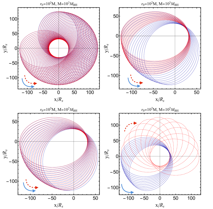
Figure 1: The orbits of EMRIs in galaxies with and without DM halos. The mass of MBHs is set as $M_{\text{BH}}=10^{6}M_{\odot}$, the eccentricity $e=0.6$, and the semi-latus rectum $p=20R_{s}$. We take the compactness $M/r_{0}$ as $10^{-2}$ and $10^{-3}$, and the total mass $M$ as $10^{2}M_{\text{BH}}$ and $10^{3}M_{\text{BH}}$. The red dashed lines show the trajectories with DM and the blue solid lines show the orbits without DM. The arrows represent the directions of orbital precessions.

To probe DM halos and study their impact on the orbits of EMRIs, we calculate the time $P$ and the orbital precession $\Delta\phi$ over one cycle when the orbital parameter $\chi$ increases by $2\pi$,

$$T =\int_{0}^{2\pi}\frac{dt}{d\chi}d\chi,$$ (21)

$$\Delta\phi =\int_{0}^{2\pi}\frac{d\phi}{d\chi}d\chi-2\pi.$$ (22)

Expanding Eqs. (17) and (18) about $R_{s}/p=0$ to the second order and substituting the results into Eqs. (21) and (22), we get

$$T =2\pi\sqrt{\frac{2p^{3}}{R_{s}}}\frac{1}{(1-e^{2})^{3/2}}\bigg{\{}1+\frac{3}{2}(1-e^{2})\frac{R_{s}}{p}+\frac{3}{2}(1-e^{2})\left[1+\frac{5}{4}(1-e^{2})^{\frac{1}{2}}\right]\left(\frac{R_{s}}{p}\right)^{2}$$

$$+\frac{M}{r_{0}}+\frac{5M^{2}}{6r_{0}^{2}}+\frac{Mp}{r_{0}^{2}(1-e^{2})}\left(e^{2}-\frac{11}{2}\right)-\frac{3Mp^{2}/{R_{s}}}{r_{0}^{2}(1-e^{2})}\bigg{\}},$$ (23)

$$\Delta\phi =3\pi\frac{R_{s}}{p}+\frac{3\pi}{8}(18+e^{2})\left(\frac{R_{s}}{p}\right)^{2}-\frac{2\pi}{1-e^{2}}\frac{Mp}{r_{0}^{2}}\left[3+\frac{1+e^{2}+2\frac{R_{s}}{p}}{(1-e^{2})^{1/2}}\right].$$ (24)

The terms with $M$ in the above Eqs. (II) and (24) come from DM halos. In the absence of DM, $M=0$, the above results (II) and (24) recover those for EMRIs with the central MBH being a Schwarzschild BH. The dominant contribution to the period $T$ in Eq. (II) is the first term, so $T$ becomes larger as the semi-latus rectum $p$ increases. However, there are positive and negative contributions from the local DM halos, the local DM halos may slow down the increase of $T$ as $p$ increases because the negative contribution in the last term in Eq. (II) and the presence of DM halos helps the increase of $T$ with $p$ if the last negative contribution is negligible. From Eq. (24), it is easy to understand that the presence of DM halo decreases the orbital procession and even retrogrades the orbital procession if the local density of DM halos $\rho_{\text{DM}}\sim M/r_{0}^{2}$ is large enough so that the third term dominates over the first two terms. As the orbit becomes larger, i.e., the semi-latus rectum $p$ increases, the orbital precession decreases and the prograde precession decreases faster in the presence of DM halos because the third term due to DM halos in Eq. (24) becomes bigger. With DM halos, the prograde-to-retrograde precession transition happens at some critial value of $p$ and then the prograde precessions change to retrograde precessions as $p$ increases further; afterwards, the retrograde precessions increase as $p$ increases. Choosing different values for the compactness $M/r_{0}$ and the total mass of DM halos $M$ and using Eqs. (II) and (24), we plot the results of the period $T$ and the orbital precession $\Delta\phi$ versus the semi-latus rectum $p$ in Fig. 2. As expected, the orbital period $T$ increases with $p$; the prograde precessions decrease with $p$ and DM halos help the decrease. For the case of $r_{0}=10^{2}M$ and $M=10^{2}M_{\text{BH}}$, the periapsis shifts change from prograde precessions to retrograde precessions at $p=60R_{s}$ and the retrograde precession increases with $p$ when $p\gtrsim 60R_{s}$.

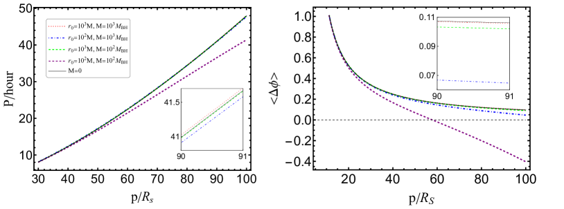
Figure 2: The results of orbital period and precession for EMRIs in galaxies with and without DM. The mass of central MBHs is set as $M_{\text{BH}}=10^{6}M_{\odot}$ and the eccentricity $e=0.6$. We take the compactness $M/r_{0}$ as $10^{-2}$ and $10^{-3}$, and the total mass $M$ as $10^{2}M_{\text{BH}}$, $10^{3}M_{\text{BH}}$ and $M=0$. The inserts show the evolution in a short time period.

From the above discussions, we see that the orbital motions of EMRIs are influenced by DM halos, and we expect that the effects of local DM halos will leave imprints on GWs so that we can probe local DM halos through the observations of GWs emitted from EMRIs.

III GWs of EMRIs in the environments of galaxies

Using the above results for the orbital motions of EMRIs, we get the leading order energy and angular momentum fluxes

$$\left<\frac{dE}{dt}\right>_{\text{GW}} \simeq\frac{32}{5}\left(\frac{\mu}{M_{\text{BH}}}\right)^{2}\left(\frac{M_{\text{BH}}}{p}\right)^{5}(1-e^{2})^{3/2}\left(1+\frac{73}{24}e^{2}+\frac{37}{96}e^{4}\right)\left(1-6\frac{M}{r_{0}}\right),$$ (25)

$$\left<\frac{dL}{dt}\right>_{\text{GW}} \simeq\frac{32}{5}\left(\frac{\mu}{M_{\text{BH}}}\right)^{2}M_{\text{BH}}\,\left(\frac{M_{\text{BH}}}{p}\right)^{7/2}(1-e^{2})^{3/2}\left(1+\frac{7}{8}e^{2}\right)\left(1-5\frac{M}{r_{0}}\right).$$ (26)

The last factors $1-6M/r_{0}$ and $1-5M/r_{0}$ are the corrections from DM halos around the MBH. Note that the effects of environmental DM halos on the losses of energy and angular momentum only depend on the compactness $M/r_{0}$ and the energy and angular momentum fluxes become smaller if the compactness is larger. In the absence of local DM halos, $M=0$, Eqs. (25) and (26) recover the standard results for eccentric binaries [63, 64]. Applying the energy and angular momentum balance equations

$$\left<\frac{dE}{dt}\right>_{\text{GW}} =-\left(\frac{dE}{dt}\right)_{\text{orbit}},$$ (27)

$$\left<\frac{dL}{dt}\right>_{\text{GW}} =-\left(\frac{dL}{dt}\right)_{\text{orbit}},$$ (28)

we get the leading order evolution of the orbital parameters $p(t)$ and $e(t)$ due to the emission of GWs,

$$\frac{dp}{dt} =-\frac{64}{5}\frac{\mu}{M_{\text{BH}}}\left(\frac{M_{\text{BH}}}{p}\right)^{3}\left(1-e^{2}\right)^{\frac{3}{2}}\left(1+\frac{7}{8}e^{2}\right)\left(1-5\frac{M}{r_{0}}\right),$$ (29)

$$\frac{de}{dt} =-\frac{304}{15}\frac{e}{p}\frac{\mu}{M_{\text{BH}}}\left(\frac{M_{\text{BH}}}{p}\right)^{3}\left(1-e^{2}\right)^{\frac{3}{2}}\left(1+\frac{121}{304}e^{2}\right)\left(1-5\frac{M}{r_{0}}\right).$$ (30)

Since the right sides of Eqs. (29) and (30) are negative, both the semi-latus rectum $p$ and the eccentricity decrease with time due to the radiation of GWs. The presence of local DM halos slows down the decrease of $p$ and $e$, the bigger the compactness $M/r_{0}$ is, the slower the semi-latus rectum $p(t)$ and the eccentricity decrease. In Fig. 3, we show the evolution of the orbital parameters $p(t)$ and $e(t)$ due to the emission of GWs. Comparing with the astrophysical environments without DM, it takes more time for EMRIs with DM halos to evolve from $p=20R_{\text{s}}$ to $p=3R_{\text{s}}$. The larger the compactness $M/r_{0}$ is, the more time it takes. The presence of DM halos also slows down the decrease rate of the eccentricity and the final eccentricity is a bit larger with larger compactness.

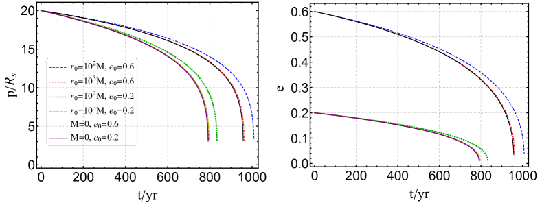
Figure 3: The evolution of the orbital parameters $p$ and $e$ from the initial $p=20R_{\text{s}}$ to $p=(3+e)R_{\text{s}}$. The mass of central MBHs is chosen as $M_{\text{BH}}=10^{6}M_{\odot}$, the mass of the SCO is $\mu=10M_{\odot}$ and the initial eccentricity is chosen as $e_{0}=0.2,0.6$. We consider two different values for the compactness of the DM halo, $M/r_{0}=10^{-2}$ and $10^{-3}$. The solid lines correspond to the cases without DM.

As discussed above, the effects of DM halos will be manifested in GW waveforms. The quadrupole formula of GWs is

$$h^{jk}=\frac{2}{d_{L}}{\ddot{I}}^{jk},$$ (31)

where $d_{L}$ is the luminosity distance between the detector and the source and $I_{jk}$ is the quadrupole moment of EMRIs. The tenser modes $h_{+}$ and $h_{\times}$ in the transverse-traceless gauge are given by

$$h_{+} =\frac{1}{2}\left(e^{j}_{X}e^{k}_{X}-e^{j}_{Y}e^{k}_{Y}\right)h_{jk},$$ (32)

$$h_{\times} =\frac{1}{2}\left(e^{j}_{X}e^{k}_{Y}-e^{j}_{Y}e^{k}_{X}\right)h_{jk},$$ (33)

where $e_{X}$ and $e_{Y}$ are the orthonormal vectors in the plane that is perpendicular to the direction from the detector to the GW source. Plugging the results for the orbital evolution obtained above into Eq. (31), we numerically calculate the time-domain GW waveforms. The time-domain plus-mode GW waveforms for EMRIs with and without DM halos are shown in Fig. 4. From Fig 4, we see that initially the difference between GW waveforms with and without DM halos is negligible. One year later, the two waveforms for EMRIs with and without DM halos are quite different.

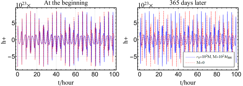
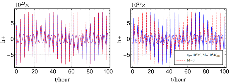
Figure 4: The time-domain plus mode GW waveforms for EMRIs with and without DM halos. The mass of central MBHs is $M_{\text{BH}}=10^{6}M_{\odot}$, the mass of the SCO is $\mu=10M_{\odot}$, the total mass of DM halos $M$ is $=10^{2}M_{\text{BH}}$, the inclination angle $\iota=\pi/6$, the luminosity distance $d_{L}=1\text{Gpc}$, the initial longitude of pericenter $\omega_{0}=0$ and the initial eccentricity $e_{0}=0.6$ at $p_{0}=20R_{s}$. $M=0$ corresponds to the case without DM halos. The left panels show the initial waveforms. The right panels show the waveforms after one year. The top panels are for $M/r_{0}=10^{-2}$ and the bottom panels are for $M/r_{0}=10^{-3}$.

In order to quantify the impact of DM halo environments on the dephasing of GW waveforms, we calculate the number of orbital cycles accumulated from time $t_{i}$ to $t_{f}$ [65, 66, 67]

$$\mathcal{N}(t)=\int_{t_{i}}^{t_{f}}\dot{\phi}(t)dt.$$ (34)

Over one-year evolution before the merger, the numbers of orbital cycles for EMRIs with and without DM halos are $\mathcal{N}_{\text{DM}}$ and $\mathcal{N}_{0}$ respectively. In Fig 5, we show the difference $\Delta\mathcal{N}=\mathcal{N}_{\text{DM}}-\mathcal{N}_{\text{0}}$ between the number of orbital cycles with and without DM halos accumulated over one year before the merger. Following [68], we choose $\Delta\mathcal{N}\sim 1\,\text{rad}$ as the threshold for a detectable dephasing. The results show that we can detect the compactness as small as $\lesssim 10^{-4}$. The results also show that eccentric orbits can help detect DM halos with smaller compactness.

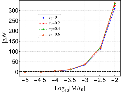
Figure 5: The difference between the orbital cycles with and without DM halos $\Delta\mathcal{N}(t)$ over one-year evolution before the merger for different compactness of halos $M/r_{0}$. The initial eccentricity $e_{0}$ is chosen at $p_{0}=20R_{s}$. The mass of central MBHs is $M_{\text{BH}}=10^{6}M_{\odot}$ and the mass of the SCO is $\mu=10M_{\odot}$. The masses of DM halos are $M=10^{2}M_{\text{BH}}$. The black dashed line corresponds to $\Delta\mathcal{N}=1\,\text{rad}$.

To distinguish the waveforms more accurately, we calculate the mismatch between GW signals emitted from EMRIs with and without DM halos. Given two signals $h_{1}(t)$ and $h_{2}(t)$, the inner product $(h_{1}|h_{2})$ is defined as

$$(h_{1}|h_{2})=2\int_{0}^{+\infty}\frac{\tilde{h}_{1}(f)\tilde{h}_{2}^{*}(f)+\tilde{h}_{2}(f)\tilde{h}_{1}^{*}(f)}{S_{h}(f)}\,df,$$ (35)

where $\tilde{h}(f)$ is the Fourier transformation of the time-domain signal $h(t)$, $\tilde{h}^{*}$ denotes the complex conjugate of $\tilde{h}$, and the SNR for the signal $h$ is $\sqrt{(h|h)}$. For LISA, the one-side noise power spectral density is [69]

$$S_{h}(f)=\frac{S_{x}}{L^{2}}+\frac{2S_{a}\left[1+\cos^{2}(2\pi\,fL/c)\right]}{(2\,\pi f)^{4}L^{2}}\left[1+\left(\frac{4\times 10^{-4}\text{Hz}}{f}\right)\right],$$ (36)

where $\sqrt{S_{a}}=3\times 10^{-15}\ \text{m s}^{-2}/\text{Hz}^{1/2}$ is the acceleration noise, $\sqrt{S_{x}}=1.5\times 10^{-11}\ \text{m/Hz}^{1/2}$ is the displacement noise and $L=2.5\times 10^{6}\text{ km}$ is the arm length of LISA [7]. The overlap between two GW signals is quantified as [60]

$$\mathcal{O}(\tilde{h}_{1},\tilde{h}_{2})=\frac{(\tilde{h}_{1}|\tilde{h}_{2})}{\sqrt{(\tilde{h}_{1}|\tilde{h}_{1})(\tilde{h}_{2}|\tilde{h}_{2})}},$$ (37)

and the mismatch between two signals is defined as

$$\text{Mismatch}=1-\mathcal{O}_{\text{max}}(\tilde{h}_{1},\tilde{h}_{2}),$$ (38)

where the maximum is evaluated with respect to time and phase shifts. The mismatch is zero if two signals are identical. Two signals are considered experimentally distinguishable if their mismatch is larger than $d/(2\,\text{SNR}^{2})$, where $d=13$ is the number of intrinsic parameters of the GW source [70, 71, 72]. Considering EMRIs with masses $(10^{6}+10)M_{\odot}$ at $d_{L}=1$ Gpc and integration time of one year before the coalescence, we calculate the mismatch between GW waveforms with and without DM halos and the results with LISA are shown in Fig 6. The SNR is about 32 for the GW signals from EMRIs considered above. The initial eccentricity $e_{0}$ is chosen at $p_{0}=20R_{s}$. As shown in Fig 6, if the compactness of DM halo $M/r_{0}$ is larger, then the mismatch between GW waveforms with and without DM halos is bigger, so more compact DM halos can be detected easier with LISA. Again eccentric orbits can detect smaller compactness. Therefore, we can use GWs from EMRIs in the environments of galaxies to test the existence of DM halos and detect the compactness of the halos $M/r_{0}$ as small as $10^{-5}$.

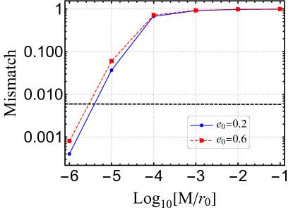
Figure 6: The results of the mismatch between GW waveforms with and without DM halos for different compactness $M/r_{0}$ and initial eccentricity $e_{0}$. The black dashed line corresponds to the threshold $d/(2\,\text{SNR}^{2})\approx 0.0072$.

IV Conclusions and Discussions

Using the analytic, static and spherically symmetric metric for a Schwarzschild black hole immersed in DM halos with Hernquist type density distribution, we derive analytic formulae for the orbital period and orbital precession for eccentric EMRIs with the environment of DM halos. The results show that the presence of DM halo decreases the orbital procession and even retrogrades the orbital procession if the local density of DM halos $\rho_{\text{DM}}\sim M/r_{0}^{2}$ is large enough. As the orbit becomes larger, the orbital precession decreases and the prograde precession decreases faster in the presence of DM halos. With DM halos, the prograde-to-retrograde precession transition happens at some critial value of $p$ and then the prograde precessions change to retrograde precessions as $p$ increases further; afterwards, the retrograde precessions increase as $p$ increases.

Taking the energy and angular momentum fluxes of GWs into consideration, we derive analytic formulae for the evolutions of the semi-latus rectum and the eccentricity. The presence of local DM halos slows down the decrease of the semi-latus rectum and the eccentricity. Comparing the numbers of orbital cycles with and without DM halos over one-year evolution before the merger, we find that DM halos with the compactness as small as $10^{-4}$ can be detected. By calculating the mismatch between GW waveforms with and without DM halos, we show that we can use GWs from EMRIs in the environments of galaxies to test the existence of DM halos and detect the compactness as small as $10^{-5}$. We also find that eccentric orbits can help detect DM halos with smaller compactness.

Binaries in the environments of galaxies are also affected by the dynamical frictions of the surrounding medium [73, 74, 75, 76, 77], and the accretion of the medium [78, 79, 46]. It is necessary to consider the effects of dynamical frictions and accretion when the medium is dense. To distinguish the effects of DM halos from other mediums (e.g. accretion disks), or modified gravity on GWs, further study is needed [43, 80, 81, 82, 68].