Probing lens-induced gravitational-wave birefringence as a test of general relativity

Abstract

Theories beyond general relativity (GR) modify the propagation of gravitational waves (GWs). In some, inhomogeneities (aka. gravitational lenses) allow interactions between the metric and additional fields to cause lens-induced birefringence (LIB): a different speed of the two linear GW polarisations ($+$ and $\times$). Inhomogeneities then act as non-isotropic crystals, splitting the GW signal into two components whose relative time delay depends on the theory and lens parameters. Here we study the observational prospects for GW scrambling, i.e when the time delay between both GW polarisations is smaller than the signal’s duration and the waveform recorded by a detector is distorted. We analyze the latest LIGO–Virgo–KAGRA catalog, GWTC-3, and find no conclusive evidence for LIB. The highest log Bayes factor that we find in favour of LIB is $3.21$ for GW$190521$, a particularly loud but short event. However, when accounting for false alarms due to (Gaussian) noise fluctuations, this evidence is below 1–$\sigma$. The tightest constraint on the time delay is $<0.51$ ms (90% C.L.) from GW$200311\_115853$. From the non-observation of GW scrambling, we constrain the optical depth for LIB, accounting for the chance of randomly distributed lenses (eg. galaxies) along the line of sight. Our LIB constraints on a (quartic) scalar-tensor Horndeski theory are more stringent than solar system tests for a wide parameter range and comparable to GW170817 in some limits. Interpreting GW190521 as an AGN binary (i.e. taking an AGN flare as a counterpart) allows even more stringent constraints. Our results demonstrate the potential and high sensitivity achievable by tests of GR, based on GW lensing.

I Introduction

The detection of gravitational waves (GW) using the LIGO–Virgo–KAGRA (LVK) detectors Aasi et al. (2015); Acernese et al. (2015); Aso et al. (2013) from mergers of compact objects Abbott et al. (2016, 2017a, 2019a, 2021a, 2021b); Nitz et al. (2020a, 2021); Venumadhav et al. (2020) has enabled precision tests of general relativity (GR) in the strong field regime Abbott et al. (2016); Abbott et al. (2019b, 2021c, 2021d). Far away from the source, GR predicts that GWs are well described as linear perturbations of the background Friedmann-Robertson-Walker (FRW) metric  Will (1998) Existing propagation tests hence typically consider modifications over the FRW background and its effect on the GW signals as measured at the detectors Ezquiaga and Zumalacárregui (2018); Arai and Nishizawa (2018); Nishizawa (2018).

GR also dictates that GWs have only two tensor polarisations ($+,\times$) which propagate independently from each other at the speed of light. However, in alternative theories of gravity, extra degrees of freedom (tensor, vector, scalar) Will (2014) can mix with GWs as they propagate, producing phenomena similar to neutrino oscillations (i.e. due to interactions between different neutrino flavors Workman and Others (2022)). In Lorentz invariant theories, the symmetries of the FRW restricts mixing effects to tensor degrees of freedom, either fundamental (e.g. in bigravity) or composite (e.g. multiple vector fields) Max et al. (2017, 2018); Belgacem et al. (2019); Jiménez et al. (2020); Ezquiaga et al. (2021a). However, inhomogeneities spontaneously break Lorentz symmetry, allowing interaction between GWs and scalar or vector degrees of freedom Ezquiaga and Zumalacárregui (2020); Dalang et al. (2021). This leads to new, testable predictions, and opens new opportunities to probe the gravitational sector beyond the FRW limit.

The evolution of GWs on an inhomogeneous background is described via propagation eigenstates: linear combinations of the interaction eigenstates ($h_{+},h_{\times}$ and perturbations of additional polarisations) with a well-defined dispersion relation (analogous to massive neutrinos). As the relation between interaction and propagation eigenstates and their speed depends on position and direction, an inhomogeneous region of space splits the original signal into several components, each arriving with a relative time delay Ezquiaga and Zumalacárregui (2020). Moreover, if deviations from GR are small, two eigenstates correspond to mostly-tensorial polarizations (linear combinations of $h_{+},h_{\times}$ plus a negligible correction distinguishing both), with a very small speed difference.

We will refer to the difference in propagation speed between the $+,\times$ polarizations as lens-induced birefringence (LIB). LIB is analogous to the way a non-isotropic crystal, such as calcite, splits light in two beams. This splitting is caused by a difference in the refractive index of the linear electromagnetic polarizations, which depends on the alignment of the polarization vector with the crystal structure. In our case birefringence is caused not by anisotropies in a crystal, but by the background configuration of additional, non-GR fields which spontaneously break Lorentz symmetry. Moreover, LIB splitting is independent of the frequency (in the high frequency approximation assumed), which would correspond to a perfectly isochromatic birefringent crystal. Because GW detectors have excellent time resolution and bad sky localization, our main observable will be the time delay between splitted signals and not their angular separation.

If the arrival time difference between the mostly-tensorial polarisations is larger than the duration of the binary merger signal then we would see only one polarisation at a time, mimicking a binary with either a zero inclination angle (face-on binary) or with $90\degree$ inclination angle (face-off binary), appearing as GW echoes. Since the detectors are more sensitive to face-on binaries, one can expect excess of near zero inclinations in case of birefringence for the population of binaries. If the delay between the polarisations is larger than typical observing runs or the amplitude of one of the polarisations decays faster than the other, e.g. in Chern-Simons gravity Okounkova et al. (2022), one would also expect an anisotropic inclination distribution. Current observations though show that the orientation distribution is consistent with being isotropic Vitale et al. (2022).

However, when the time delay is less than the duration the signal, the GW waveform would be distorted or “scrambled” due to the interference of both polarisations. Note that this effect is frequency-independent, and hence distinguishable from a different dispersion relation for the $+$ and $\times$ modes or the circularly polarized combinations (L-R), as predicted in GR de Rham and Tolley (2020); Andersson et al. (2021); Oancea et al. (2022) and alternative theories Wang et al. (2022); Haegel et al. (2022); Bombacigno et al. (2022). As it is not suppressed by the frequency, LIB is the dominant effect in the high-frequency limit for theories in which this effect is present.

Our study analyzes for the first time arrival time difference ($\Delta t_{12}$) between the two polarisation states due to different propagation speeds (frequency-independent dispersion relations) as a result of LIB. This is a new, model-independent test of a basic prediction of GR. We use these generic results to constrain GW lensing effects beyond GR, for example in scalar-tensor theories with derivative interactions  Ezquiaga and Zumalacárregui (2020).

LIB signatures are not linked to a specific regime of gravitational lensing in GR, such as strongly magnified or multiple images. The scale on which LIB can be observed is very sensitive to the theory parameters and independent of the Einstein radius $R_{E}$, which characterizes the regimes of gravitational lensing. Hence, for sufficiently strong deviations from GR, LIB can be detected for impact parameters much larger than $R_{E}$, typically associated to weak lensing. Therefore, LIB-tests can be applied to all the GW detections. In addition, LIB can be important for lenses very close to the source or the observer, for which $R_{E}$ vanishes. This is particularly interesting for sources merging near massive objects (e.g. a supermassive BH) since the background configuration of the additional fields enhances LIB.

The rest of the paper is organised as follows. In Sec. II we describe our LIB waveform model, methods for data analysis and introduce parameterized LIB observation probabilities. In Sec. III, we perform the birefringence test over a set of simulated GW events, and then to real events using the Bayesian model selection framework. In Sec. IV, we study the implications of the results in constraining LIB probabilities and beyond-GR theories. Finally, in Sec. V we summarize the main results and discuss future prospects.

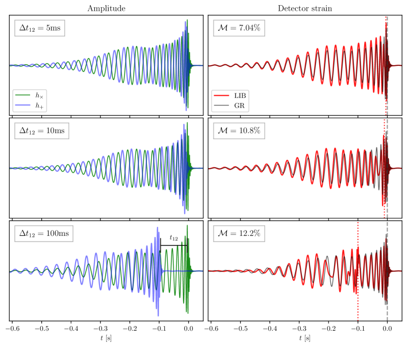
Figure 1: GW polarisations (left) and detector strain (right) for a CBC $(30+30)M_{\odot}$ with birefringent time delays $\Delta t_{12}=5,10,100$ ms (top to bottom). The sky localization and detector orientation correspond to $F^{+}=-0.38$, $F^{\times}=0.71$ and LIB strain is given by Eq.  5

II Method

In GR, GWs have only two polarisations $(+,\times)$ which propagate independently at the speed of light over the background FRW metric. A given ground-based detector $I$ measures the GW signal, $h(t)$ as a linear combination of these polarisations Veitch et al. (2015),

$$h_{I}(t)=F^{+}_{I}h_{+}(t)+F^{\times}_{I}h_{\times}(t)$$ (1)

where, $F^{+}_{I},F^{\times}_{I}$ are the detector antenna pattern functions. In the case of compact binary coalescence (CBC), the relative amplitude of the polarisation modes depends on the inclination and polarisation angles of the binary w.r.t to the line of sight, and also depends on the sensitivity of the detector for the source location at the time of arrival. The overall amplitude of the signal is inversely proportional to the luminosity distance of the source. Masses and spins of the source dictate the frequency evolution of the signal and its amplitude.

II.1 Parameterized Lens-induced Birefringence Waveforms

When there is any inhomogeneity along the travel path of a GW, e.g. an intervening galaxy, the GW can be gravitationally lensed. Gravitational lensing of a GW can produce multiple images of the original signal (strong lensing) or cause distortions (microlensing), but, in GR, both polarisations are affected in the same way, i.e. the polarisation rotation is negligible for any sensible astrophysical lens Ezquiaga et al. (2021b); Cusin and Lagos (2020). However, in alternative theories of gravity the additional fields can couple with the tensor polarizations around the lens and modify the GW propagation eigenstates. These eigenstates are a linear combination of original GW polarisations that evolve independently, each with a different speed, thus reaching the detectors at different times. We will assume spherically symmetric lenses, focus on the limit of small deviations from GR, so the mostly-metric propagation eigenstates correspond to linear combinations of $h_{+},h_{\times}$ (depending on the projected angle between the lens and the source), and neglect the additonal eigenstates (See Ref. Ezquiaga and Zumalacárregui (2020) and footnote 1).

This class of LIB of GWs can be captured in a phenomenological manner as proposed in Ref. Ezquiaga and Zumalacárregui (2020). After diagonalizing the propagation equations, the propagation eigenstates can be computed and one gets the transformation matrix ${\mathcal{S}}$ relating the polarisation amplitudes in GR and after the LIB:

$$[h_{+},h_{\times}]^{T}_{\text{LIB}}=\mathcal{S}[h_{+},h_{\times}]^{T}_{\mathrm{GR}}$$ (2)

where

$${\mathcal{S}}=\hat{\mathcal{M}}\ \text{diag}(1,\Delta)\hat{\mathcal{M}}^{-1}\,,$$ (3)

$$\hat{\mathcal{M}}=\left[\begin{array}[]{cc}-\sin(2\phi_{\mathrm{lens}})&\cos(2\phi_{\mathrm{lens}})\\ \cos(2\phi_{\mathrm{lens}})&\sin(2\phi_{\mathrm{lens}})\end{array}\right]\,,$$ (4)

and $\Delta=e^{-i\omega\Delta t_{12}}$ with $\Delta t_{12}$ is the time delay between the polarisations and $\phi_{\mathrm{lens}}$ as the angle between the lens and the source, relative to the direction of GWs propagation that dictates the polarisation mixing.

It is easy to note that for $\phi_{\mathrm{lens}}=\pi/2$, $\mathcal{S}=\mathrm{diag}(1,\Delta)$, hence the signal observed by the detectors will just be superposition of $(+,\times)$ arriving at different times.

$$h_{I}^{\text{LIB}}(t)=F^{+}_{I}h_{+}(t)+F^{\times}_{I}h_{\times}(t-\Delta t_{12})$$ (5)

whereas, if $\Delta t_{12}=0$ the LIB waveform morphology will be identical to the GR one, independent of $\phi_{\mathrm{lens}}$. Fig. 1 compares GR v/s LIB waveform polarisations and the detector strains for various values $\Delta t_{12}$. Under LIB, the polarisations interfere leading to waveform distortions.

Since lensing is an environmental effect which can occur through any local inhomogeneity in the path of GWs, the parameters $\Delta t_{12}$ and $\phi_{\rm lens}$ are expected to vary between GW events. The time delay distribution depends on the theory and the (usually unknown) lens properties and the configuration relative to the source. In general, one can only predict the probability of the birefringence parameters given a gravitational theory and matter distribution (unless further information or assumptions are employed about the source’s location or the signal’s trajectory), see Sec. II.4. This is in stark contrast to other tests of GW propagation (that are done with individual GW events) in which deviations represent a fundamental property of gravity (eg. massive graviton dispersion relations) and are thus the same across all events and only depend on their distance Will (2014).

II.2 Template Mismatch Studies

In order to quantify distortions due to GW birefringence, we calculate the mismatch between the GR and LIB waveforms as seen the LIGO-Virgo detectors. At each detector ($I$), the mismatch between the injected waveform ($h_{I}^{\mathrm{inj}}$) and the recovery waveform ($h_{I}^{\mathrm{rec}}$) is given by:

$$M_{I}=1-\frac{(h_{I}^{\mathrm{inj}}|h_{I}^{\mathrm{rec}})}{||h_{I}^{\mathrm{inj}}||.||h_{I}^{\mathrm{rec}}||}$$ (6)

where, $(\cdot\mid\cdot)$ symbolises the noise-weighted inner product:

$$(a~{}|~{}b)\equiv 2\int_{f_{\mathrm{min}}}^{f_{\mathrm{max}}}\frac{\tilde{a}(f)\tilde{b}^{*}(f)}{S_{n}(f)}df\,.$$ (7)

Here, $\tilde{a},\tilde{b}$ represent the Fourier transform of the time series $a(t),b(t)$; $[f_{\mathrm{min}},f_{\mathrm{max}}]$ is the frequency range over which the inner product is evaluated; ^∗ represents complex conjugation and $S_{n}(f)$ is the colored Gaussian noise power spectral density (PSD) at the detector. The norm $||h||=\sqrt{(h|h)}$ is the optimal SNR of a waveform. We define the total mismatch ($\mathcal{M}$) for network of detectors as the signal-to-noise ratio (SNR, $\rho_{I}$) squared weighted average of individual detector matches,

$$\mathcal{M}=\frac{\sum_{I}\rho_{I}^{2}M_{I}}{\sum_{I}\rho_{I}^{2}}$$ (8)

Note that the mismatch is a normalized quantity and is maximised over time and phase shifts. Thus, the mismatch quantifies differences in morphology between the signals. Whereas, during the parameter estimation (PE) from GW signals both the mismatch and SNR play a role as the log-likelihood $\propto\mathcal{M}{\sum_{I}\rho_{I}^{2}}$ around the maximum likelihood parameters. We first wish to quantify the overall detectability of the birefringence. Later, we will estimate parameters using Bayesian inference, accounting for correlations between all parameters.

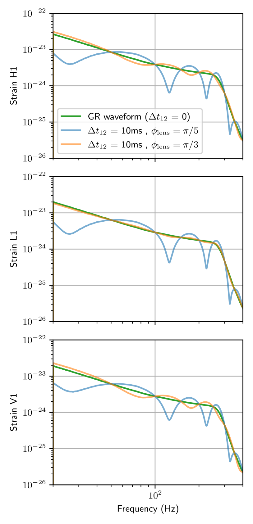
Figure 2: GR and LIB detector frame waveform amplitudes in frequency domain of GW150914-like CBC. The birefringence leads to additional frequency modulations and distorts the GR waveform. The magnitude of these distortions are however dependent on the two parameters: $\Delta t_{12}$ and $\phi_{\mathrm{lens}}$.

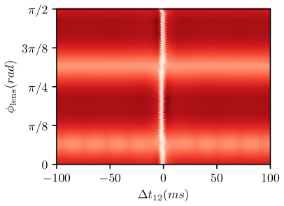
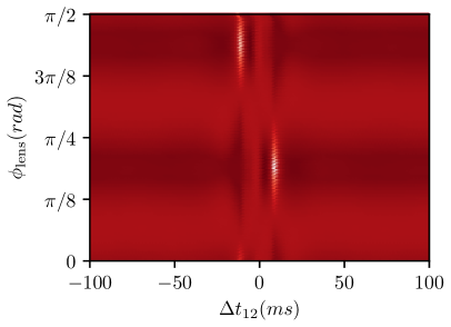
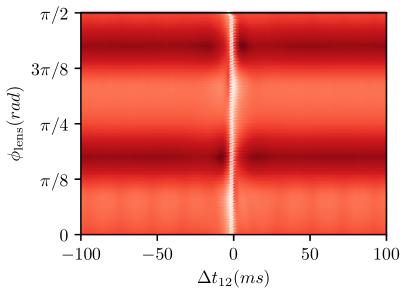
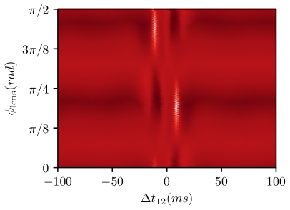
Figure 3: Mismatch between GR and LIB waveforms for GW150914-like CBC (top) and GW190814-like CBC (bottom). left pannel: GR injection i.e. $\Delta t_{12}^{\mathrm{inj}}=0$ and $\phi_{\mathrm{lens}}^{\mathrm{inj}}=0$. the mismatch is minimum for $\Delta t_{12}^{\mathrm{rec}}\simeq 0$. right pannel: a LIB injection with $\Delta t_{12}^{\mathrm{inj}}=10$ ms and $\phi_{\mathrm{lens}}^{\mathrm{inj}}=\pi/5$.The mismatch is minimum at $\Delta t_{12}^{\mathrm{rec}}\simeq\pm 10\mathrm{ms}$ and $\phi_{\mathrm{lens}}^{\mathrm{rec}}\simeq\pi/5,\pi/4+\pi/5$.

Fig. 2 shows frequency domain LIB and GR waveforms for a GW150914-like CBC. The waveforms are generated using the approximant IMRPhenomXPHM Pratten et al. (2021), as implemented in the LALSimulation module of the LALSuite software package LIGO Scientific Collaboration (2018). The waveforms are then projected onto the LIGO and Virgo detectors using their antenna pattern functions, as implemented in the bilby Ashton et al. (2019) software package. The LIB waveforms have additional frequency modulations which depend on the two parameters: $\Delta t_{12}$ and $\phi_{\mathrm{lens}}$ (see II.1). Therefore we calculate the mismatch between the GR and LIB waveforms, keeping all the other parameters identical and fixed for the two waveforms. In practice, we calculate ${M_{I}}$ using pycbc.filter Nitz et al. (2020b) module. The detector noise is generated using the zero-detuned high-power PSDs of Advanced LIGO and Advanced Virgo at their design sensitivities The Virgo Collaboration (2012); aLI (2018).

We consider two systems of binaries, one whose parameters resemble to that of the first CBC detection GW150914 and other of a higher mass-ratio CBC GW190814 where the presence of higher-order modes (HoMs) of GWs are significant. For both the systems, we inject a GR and a LIB waveform and recover with LIB waveform to calculate the mismatch. The parameters for both the CBCs are mentioned in Appendix A

Fig. 3 shows mismatches for a GW150914-like CBC (top) and GW190814-like CBC (bottom). As expected for a GR injection i.e. $\Delta t_{12}^{\mathrm{inj}}=0$ and $\phi_{\mathrm{lens}}^{\mathrm{inj}}=0$, the mismatch is minimum for $\Delta t_{12}^{\mathrm{rec}}\simeq 0$, for all $\phi_{\mathrm{lens}}$ as expected from Eq.  3. Additionally, the local minimum of mismatch is at $\phi_{\mathrm{lens}}^{\mathrm{rec}}\simeq\pi/3$, which could be because of vanishing polarisation ($+$ or $\times$) as seen at the detectors which further makes the mismatch independent of the time delay $\Delta t_{12}$. The waveform plots in Fig. 2 confirms this as the $\phi_{\mathrm{lens}}^{\mathrm{rec}}\simeq\pi/3$ waveform resembles the GR ones more as compared to the $\phi_{\mathrm{lens}}^{\mathrm{rec}}\simeq\pi/5$, especially in the Livingston (L1) detector for GW150914-like CBC.

We also checked the mismatch for the LIB injections (right panel Fig. 3) with $\Delta t_{12}^{\mathrm{inj}}=10$ ms and $\phi_{\mathrm{lens}}^{\mathrm{inj}}=\pi/5$ and the mismatch is minimum at, $\Delta t_{12}^{\mathrm{rec}}\simeq\pm 10$ ms and $\phi_{\mathrm{lens}}^{\mathrm{rec}}\simeq\pi/5,\pi/4+\pi/5$. We can infer the degeneracy between $\Delta t_{12}$ and the coalescence time ($t_{c}$) as follows, from Eq. (1)-(4) if $\phi_{\mathrm{lens}}\rightarrow\phi_{\mathrm{lens}}+\pi/4$ and $\Delta\rightarrow 1/\Delta$ then, one finds $S\rightarrow S/\Delta$, which implies that the modification at $(\Delta t_{12},\phi_{\mathrm{lens}},t_{c})$ is the same as at $(-\Delta t_{12},\phi_{\mathrm{lens}}+\pi/4,t_{c}+\Delta t_{12})$. Note that, this degeneracy stems from the fact that we do not know the composition of $h_{+,\times}$ before it encounters the lens. Additional information about the source could break this degeneracy, but we leave these investigations for the future.

II.3 Bayesian Inference

Bayesian model selection allows us to assign evidences for various hypotheses pertaining to the observed data, and also derive posterior probability distributions of the model parameters conditioned on individual hypotheses. Given the set of data $\{d\}$ from a network of detectors, the marginalized likelihood (or, Bayesian evidence) of the hypothesis $\mathcal{H_{A}}$ can be computed by

$$P(\{d\}|\mathcal{H_{A}})=\int d{\bm{\theta}}P({\bm{\theta}}|\mathcal{H_{A}})\,P(\{d\}|{\bm{\theta}},\mathcal{H_{A}}),$$ (9)

where ${\bm{\theta}}$ is a set of parameters that describe the signal under hypothesis $\mathcal{H_{A}}$ (including the masses and spins of the compact objects in the binary, location and orientation of the binary and the arrival time and phase of the signal), $P({\bm{\theta}}|\mathcal{H_{A}})$ is the prior distribution of ${\bm{\theta}}$ under hypothesis $\mathcal{H_{A}}$, and $P(\{d\}|{\bm{\theta}},\mathcal{H_{A}})$ is the likelihood of the data $\{d\}$, given the parameter vector ${\bm{\theta}}$ and hypothesis $\mathcal{H_{A}}$. Given the hypothesis $\mathcal{H_{A}}$ and data $\{d\}$, we can sample and marginalize the likelihood over the parameter space using an appropriate stochastic sampling technique such as nested sampling Skilling (2006).

Bayesian model selection allows us to compare multiple hypotheses. For e.g., the odds ratio $\mathcal{O}^{\text{LIB}}_{\mathrm{GR}}$ is the ratio of the posterior probabilities of the two hypotheses LIB and GR. When $O^{\text{LIB}}_{\mathrm{GR}}$ is greater than one then hypothesis LIB is preferred over GR and vice versa. Using Bayes theorem, the odds ratio can also be written as the product of the ratio of the prior odds $P^{\text{LIB}}_{\mathrm{GR}}$ of the hypotheses and the likelihood ratio, or Bayes factor $\mathcal{B}^{\text{LIB}}_{\text{GR}}$:

$$\mathcal{O}^{\text{LIB}}_{\mathrm{GR}}: =\frac{P(\mathcal{H}^{\text{LIB}}|\{d\})}{P(\mathcal{H}^{GR}|\{d\})}=\frac{P(\mathcal{H}^{\text{LIB}})}{P(\mathcal{H}^{GR})}\times\frac{P(\{d\}|\mathcal{H}^{\text{LIB}})}{P(\{d\}|\mathcal{H}^{GR})}$$ (10)

$$=\mathcal{P}^{\text{LIB}}_{\mathrm{GR}}\times\mathcal{B}^{\text{LIB}}_{\text{GR}}$$ (11)

Since GR has been tested well in a variety of settings, our prior odds are going to be highly biased towards it, i.e., $\mathcal{P}^{\text{LIB}}_{\mathrm{GR}}\ll 1$. Hence, in order to claim evidence of birefringence the corresponding Bayes factor supporting the LIB hypothesis has to be very large. Since the Bayes factor is the only quantity that is derived from data, for the rest of the paper, we focus on the Bayes factor, i.e. the ratio of evidences under the two hypothesis.

The waveforms under the GR and LIB hypotheses at each detector is the same way as described in Sec. II.2. We use the standard Gaussian likelihood model for estimating the posteriors of the parameters under different hypotheses (see, e.g., Veitch et al. (2015)). We use uniform priors in redshifted component masses of the binary, isotropic sky location (uniform in $\alpha,\sin\delta$) and orientation (uniform in $\cos\iota,\phi_{0}$), uniform in polarisation angle $\psi$, and a prior $\propto d_{L}^{2}$ on luminosity distance. Additionally for the LIB hypothesis, we choose the priors on $\Delta t_{12}$ as uniform $\in[-100,100]$ ms and $\phi_{\mathrm{lens}}$ as uniform $\in[0,\pi/2]$. To estimate the posterior distribution and evidences for the GR and LIB hypotheses, we use the open-source parameter estimation package bilby package Ashton et al. (2019) coupled with the dynamical nested sampler dynesty Speagle (2020).

II.4 Lensing Probabilities

The (non-)observation of birefringence can help us put constraints on theories beyond GR that predict LIB. According to GR, the strong lensing of GWs caused by galaxies occurs when sources lie inside the Einstein radius of the lens, which depends on lens mass and profile. This is the relevant scale determining the probability of lensing. However, birefringence beyond GR is in principle independent of the ratio between the impact parameter and the Einstein radius, changing the probability of observing LIB compared to strong lensing. It is thus possible to have LIB time delays without multiple images, but birefringence could also occur for strongly lensed GWs, in which case it applies to each image separately, as typical time delays between images will be larger than $\Delta t_{12}$ Ezquiaga and Zumalacárregui (2020).

Assuming that the lenses are randomly distributed, birefringence detection is described by Poisson statistics. A series of observations with $L$ lensed and $U$ unlensed GW events has an associated probability,

$$P=\exp\Big{(}{-\sum_{i}^{U}\lambda_{i}}\Big{)}\prod_{j}^{L}\left(1-e^{-\lambda_{j}}\right)\,.$$ (12)

The result depends on LIB rate for the $i^{th}$ event: $\lambda_{i}=\int dz_{s}d\vec{p}_{L}d\vec{p}_{S}\tau(z_{s},\vec{p}_{L})\mathcal{P}_{i}(z_{s},\vec{p}_{S})P(\vec{p}_{S},\vec{p}_{L})$. Here $S,L$ denote parameters corresponding to the source and lens/theory (i.e. beyond GR), $\mathcal{P}_{i}$ is the posterior distribution of the source parameters and $P$ is the prior, which includes relations between parameters (i.e. the measured $\Delta t_{12}$ as a function of lens mass and beyond-GR parameters). The birefringence optical depth, $\tau(z_{s},\vec{p}_{L})$ is the fraction of the sky for which LIB is detectable for sources at a redshift $z_{s}$. Hereafter we will assume the posterior to be sharply peaked at the mean source redshift $z_{s}$ and include the integration on the lens model parameters ($\vec{p}_{L}$) in the definition of the optical depth, so $\lambda_{i}\approx\tau(z_{s,i})$. If birefringence is excluded in all events, the probability only depends on the total optical depth $\tau_{tot}\approx\sum_{i=1..N}\tau_{i}\approx\sum_{i=1..N}\lambda_{i}$. In Appendix B we will comment on opportunities to study GW birefringence beyond the Poisson statistics.

The lensing optical depth $\tau\left(z_{s}\right)$ depends on the angular cross section $\hat{\sigma}\left(z_{s},\vec{p}_{L}\right)$ and the density of lenses $\hat{n}\left(\vec{p}_{L}\right)$ Xu et al. (2022). In the following we will explicitly write the lens redshift $z_{L}$ and let $\vec{p}_{L^{\prime}}$ denote the remaining properties (i.e. lens mass & theory parameters). The total density of lenses at redshift $z_{L}$ is then $\int\hat{n}\left(z_{L},\vec{p}_{L^{\prime}}\right)d\vec{p}_{L^{\prime}}$. The optical depth is computed directly by adding-up the cross-sections weighted by the density at different redshifts, i.e.

$$\tau\left(z_{s}\right)=\int_{0}^{z_{s}}dz_{L}\int d\vec{p}_{L^{\prime}}\frac{dV_{c}}{\delta\Omega dz_{L}}\hat{n}\left(z_{L},\vec{p}_{L^{\prime}}\right)\hat{\sigma}\left(z_{s},z_{L},\vec{p}_{L^{\prime}}\right)$$ (13)

where $dV_{c}=\delta\Omega D_{L}^{2}\frac{dz}{(1+z)H(z)}$ is the physical volume given the solid angle $\delta\Omega$, angular diameter distance to the lens $D_{L}$ and the Hubble parameter $H(z)$. For simplicity, we will assume point mass lenses of mass $M$ throughout. In GR, the lensing cross-section is $\sigma=\pi\theta_{E}^{2}$, where $\theta_{E}=R_{E}/D_{L}=(\frac{4GMD_{LS}}{c^{2}D_{L}D_{S}})^{1/2}$ is the Einstein angle, $D_{S}$ is the distance to the source from the earth and $D_{LS}$ is the distance between lens and source.

The relation between the LIB-time delays, the theory parameters and the configuration of the lensed system is complex (See Sec. VI of Ref. Ezquiaga and Zumalacárregui (2020) for a worked-out example in a viable Horndeski theory). For this reason we will first consider two phenomenological models with generic dependences of lensing cross section. As a first example, we will assume that the relevant LIB scale is proportional to the Einstein angle, $\theta^{E}_{X}=\alpha_{X}\theta_{E}$, so that the cross section becomes

$$\sigma^{E}_{X}=\pi\alpha_{X}^{2}\theta_{E}^{2}\,.$$ (14)

Then the optical depth is given by Eq. (74) in Ref. Ezquiaga and Zumalacárregui (2020) where the lenses have been assumed point-like.

Under these assumptions, lensing probabilities are independent of the mass function.

In our second example we assume that the relevant LIB scale is given by a constant physical scale associated to each halo. Moreover, we assume that this scale depends on the halo mass as a power law. Accordingly, the cross-section reads,

$$\sigma_{\rm ph}=\pi\frac{R_{12}^{2}}{D_{L}^{2}}\left(\frac{M}{10^{12}M_{\odot}}\right)^{2n}\,.$$ (15)

The scale $R_{12}$ fixes the probability of lensing for halos with $M=10^{12}M_{\odot}$, while $n$ allows us to extrapolate to different halo masses. Below we will discuss some cases of interest.

We now generalize the expression for the optical depth presented in Ref. Ezquiaga and Zumalacárregui (2020) (Eq. 76) to include a realistic halo mass function. The optical depth from Eq. (15) is given by

$$\tau^{\rm ph}(z_{s},n)=\Omega_{M}h\left(\frac{R_{12}}{22\rm kpc}\right)^{2}\hat{\tau}(z_{s},n)\,,$$ (16)

where

$$\begin{multlined}\hat{\tau}(z_{s},n)=\int_{0}^{z_{s}}dz\frac{(1+z)^{2}}{H(z)/H_{0}}\int d\log(M)\\ \times\left(\frac{M}{10^{12}M_{\odot}}\right)^{2n-1}{f(M,z)}.\end{multlined}\hat{\tau}(z_{s},n)=\int_{0}^{z_{s}}dz\frac{(1+z)^{2}}{H(z)/H_{0}}\int d\log(M)\\ \times\left(\frac{M}{10^{12}M_{\odot}}\right)^{2n-1}{f(M,z)}.$$ (17)

Here $f(M,z)=\frac{M^{2}}{\rho_{0}}\frac{d\hat{n}}{dM}$ is the scaled differential mass function (dimensionless) with $\rho_{0}$ as the matter density of universe at $z=0$. We will use the Tinker et al. form Tinker et al. (2008) as implemented in the Colossus package Diemer (2018). As our approach is phenomenological, we assume a Planck $\Lambda$CDM cosmology Aghanim et al. (2020). The true optical depth of a consistent LIB model will typically depend more strongly on the theory parameters (e.g. entering Eq. (15) via $R_{12}$) than on the precise values of $H(z),f(M,z)$ of the underlying LIB cosmology, including the effects of deviations from GR in cosmological expansion and structure formation. This is the case for the example theory discussed in Sec. IV.2: GW lensing effects are orders of magnitude more sensitive than solar-system tests (cf. Fig. 8), in turn more stringent than current cosmological observations Zumalacarregui (2020); Alonso et al. (2017) (for theories without a screening mechanism).

In addition to the Einstein radius scaling, Eq. (14), we will consider three cases of interest:

• $n=1$: the physical scale is proportional to the total halo mass, much like the Schwarzschild radius. The rates are dominated by large masses and saturate at $z_{s}\gtrsim 1$, as the more massive halos are exponentially suppressed at early times. This case captures the dependence of the time delay in a Horndeski model (Sec. IV.2).

• $n=1/2$: the scale has the same mass scaling as the Einstein radius and leads to rates independent of $M$. However, the overall redshift dependence is different, as $R_{E}$ depends also on $D_{S},D_{LS}$.

• $n=1/3$: this mass scaling favors lighter halos and thus grows very rapidly with redshift. It is motivated by the mass-dependence of the Vainshtein radius $R_{V}$, i.e. the classical strong-coupling scale Vainshtein (1972). For $n=1/3$ the contribution from lighter halos diverges and a low mass cutoff needs to be included (we will take $M>10^{7}M_{\odot}$). We will see this mass dependence when considering a binary merging near an active galactic nuclei in a Horndeski theory (Sec. IV.3).

The optical depths for each of the cases as a function of the source redshift are plotted in Fig. 7. Note that these phenomenological models assume that the cross section is independent of $\Delta t_{12}$, and thus common for all the analyzed events. Dependence in the time delay can be included, e.g. by multiplying Eqs. (14), (15) by a factor $(\Delta t_{12}/10{\rm\mathrm{ms}})^{-k}$. For the sake of simplicity, we will not include this dependence and instead interpret the obtained values of $\alpha_{X}$, $R_{12}(n)$ at the median 95% c.l. from all analyzed events.

III Results

In order to test our method and understand the observing capabilities, we first apply our pipeline to injections. We then proceed to analyse the latest GW catalog (GWTC-3).

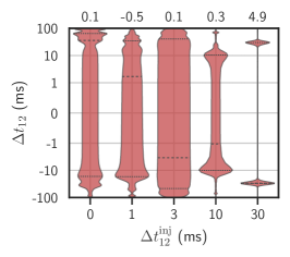
(a) $SNR$ $10$

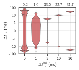
(b) $SNR$ $15$

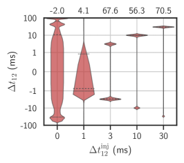
(c) $SNR$ $20$

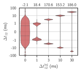
(d) $SNR$ $30$

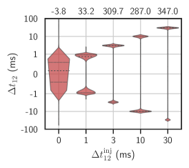
(e) $SNR$ $40$

Figure 4: Signal-to-noise ratio (SNR) dependence of $\Delta t_{12}(\mathrm{ms})$ posteriors and the $\log\mathcal{B}^{\text{LIB}}_{\text{GR}}$ (upper-x axis) for the GW150914-like injections with different values of $\Delta t_{12}^{\mathrm{inj}}$ (lower-x axis) and $\phi_{\mathrm{lens}}^{\mathrm{inj}}=\pi/5$. Time delays ($\Delta t_{12}$) as small as $1ms$ are recovered well with SNR 30 & 40 signals, and for SNR 10 signals time delays $<30ms$ are not measurable. Both model selection and time delay measurements (without the symmetry around $\Delta t_{12}=0$) improve with increase in SNR.

III.1 Injections

We inject GW150914-like signals in simulated Gaussian noise with $\Delta t_{12}^{\mathrm{inj}}\in\{0,1,3,10,30\}$ ms and $\phi_{\mathrm{lens}}^{\mathrm{inj}}=\pi/5$ rad and recover them by running the parameter estimation routines under the GR and LIB hypothesis, as mentioned in Sec. II.3. This allows us to compute the Bayes factors $\mathcal{B}^{\text{LIB}}_{\text{GR}}$ to compare the two hypothesis for each injection.

The injections are set to have $\mathrm{SNR}\in\{10,15,20,30,40\}$. These SNRs are achieved by inversely scaling the luminosity distance ($d_{L}$) of the injections. Fig. 4 shows the violin plots and the $\log$ Bayes Factors for these injections. The posteriors on $\phi_{\mathrm{lens}}$ are uninformative in all the cases and hence not shown in the figure. LIB time delays ($\Delta t_{12}$) as small as 1 ms are recovered well with SNR 30 and 40 signals, whereas for SNR 10 signals time delays $<30$ ms are not measurable. As one would expect, only with $\Delta t_{12}^{\mathrm{inj}}=0$, i.e. GR injection the $\log\mathcal{B}^{\text{LIB}}_{\text{GR}}<0$, i.e. consistent with the GR hypothesis, except for the SNR 10 case where $\log\mathcal{B}^{\text{LIB}}_{\text{GR}}=0.1$ is within the intrinsic sampling error on the calculation of evidence. For $\Delta t_{12}^{\mathrm{inj}}\in\{1,3,10,30\}$ ms we find that $\log\mathcal{B}^{\text{LIB}}_{\text{GR}}>0$, i.e. consistent with the LIB hypothesis for all the SNRs except 10. Hence, both model selection and sensitivity to measure the time delays improve with an increase in SNR.

We also note that the time delays are measurable up to a symmetry around $\Delta t_{12}=0$. This is because LIB waveform, Eq. (3), is identical at $(\Delta t_{12},\phi_{\mathrm{lens}},t_{c})$ and $(-\Delta t_{12},\phi_{\mathrm{lens}}+\pi/4,t_{c}+\Delta t_{12})$, which we also saw during mismatch studies with LIB injections, see right panel of Fig.  3. It is possible that for asymmetric and inclined binaries with significant HoMs a better measurement of $\phi_{\mathrm{lens}}$ could break the $\Delta t_{12}$ parity as well, however, this needs to be investigated further and is left for future studies.

Overall, as the sensitivity of the detectors improve we shall be able to measure the birefringence time delays as small as $1$ ms. On the other hand, in the absence of birefringence we expect to see $\Delta t_{12}$(s) posteriors which are consistent with the GR value, i.e. zero and bayes factors that favour the GR hypothesis. Most events in GWTC-3 have SNR $<30$. The time delay posteriors are hence expected to be broad, however the Bayes factors should already indicate whether LIB is present or not.

III.2 GWTC-3 Events

We now analyse 43 CBC events from the GWTC-3, that have low detection false alarm rate, $\mathrm{FAR}\lesssim 10^{-3}\ \mathrm{yr}^{-1}$. These are also the events that are considered for other tests of GR performed previously Abbott et al. (2016); Abbott et al. (2019b, 2021c, 2021d).

Fig. 5 shows the $\Delta t_{12}$ posteriors and the $\log$ Bayes Factors for the real events. We find that for almost all the events the $\Delta t_{12}$ posteriors are broad containing zero, i.e. consistent with GR. This is mostly due to the low SNRs of the events, as seen in our injection study. We also find the tightest 90% credible bounds on $|\Delta t_{12}|\lesssim 0.51$ ms coming from the event GW200311_115853 which has reasonably high SNR ($\simeq 17.8$) and moderate redshift ($z\sim 0.23$) as compared to other events. As expected $\phi_{\mathrm{lens}}$ posteriors are uninformative for almost all the events.

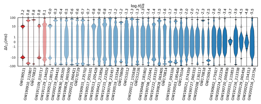
Figure 5: lens-induced birefringence (LIB) test of GWTC-3 events Abbott et al. (2021b). We show the posteriors on $\Delta t_{12}(\mathrm{ms})$ and Bayes Factors $\log\mathcal{B}^{\text{LIB}}_{\text{GR}}$ (upper $x$-axis). Events with positive Bayes factors are highlighted in red.

38 out of 43 events resulted in $\log\mathcal{B}^{\text{LIB}}_{\text{GR}}<0$, and hence consistent with the GR hypothesis. Only a few events showed preference to LIB hypothesis ($\log\mathcal{B}^{\text{LIB}}_{\text{GR}}>0$), with highest one for GW190521 (3.21) and then GW190910_112807 (0.8), GW170823 (0.8), GW191109_010717 (0.7) & GW191129_134029 (0.1).

The Bayes factors are known to be prior dependent and its value does not signify the confidence in preferring one hypothesis over the other, but rather the preference of one hypothesis over the other given a set of prior assumptions. The model with extra parameters (LIB) could be either fitting the noise or the signal, therefore we take a frequentist approach to determine the significance by considering different realisations of noise. We focus on the event with the highest Bayes factors (GW190521) and estimate its significance. We generate the background distribution of Bayes factors by injecting GR signals in Gaussian noise using the power spectral density around the trigger time. To calculate the false alarm probability corresponding to the observed Bayes Factor for the event GW190521, we simulate a hundred GR injections, whose parameters are taken from the posteriors of GW190521 event for the GR hypothesis. Fig. 6 shows the background distribution of the Bayes factors and the corresponding false alarm probability (FAP). The FAP corresponding to each $\mathcal{B}^{\text{LIB}}_{\text{GR}}=\kappa$ is calculated as the fraction of the background events having $\mathcal{B}^{\text{LIB}}_{\text{GR}}>\kappa$. We find that for the observed $\log\mathcal{B}^{\text{LIB}}_{\text{GR}}=3.2$ for GW190521 is $0.48$, i.e. its significance is less than $1\sigma$.

It is to be noted that GW190521 is a remarkably loud but short ($<100$ ms) signal, being easily fit by widely different hypotheses such as head on-collision of a boson star Calderón Bustillo et al. (2021) or left-right (L-R), frequency-dependent birefringence Wang et al. (2022). For the interested reader, in Appendix C (Fig. 10), we also plot posteriors and the waveforms corresponding to the maximum a posteriori parameters for both the hypothesis, over the whitened signals observed at each detector. The plots show that the LIB hypothesis is also fitting the noise, and might therefore give a high Bayes factor, $\mathcal{B}^{\text{LIB}}_{\text{GR}}$. The other events with $\mathcal{B}^{\text{LIB}}_{\text{GR}}>0$ are also show similar behavior and as their preference for LIB is marginal, we conclude that none of the events have any significant Bayes factor and find no strong evidence for birefringence.

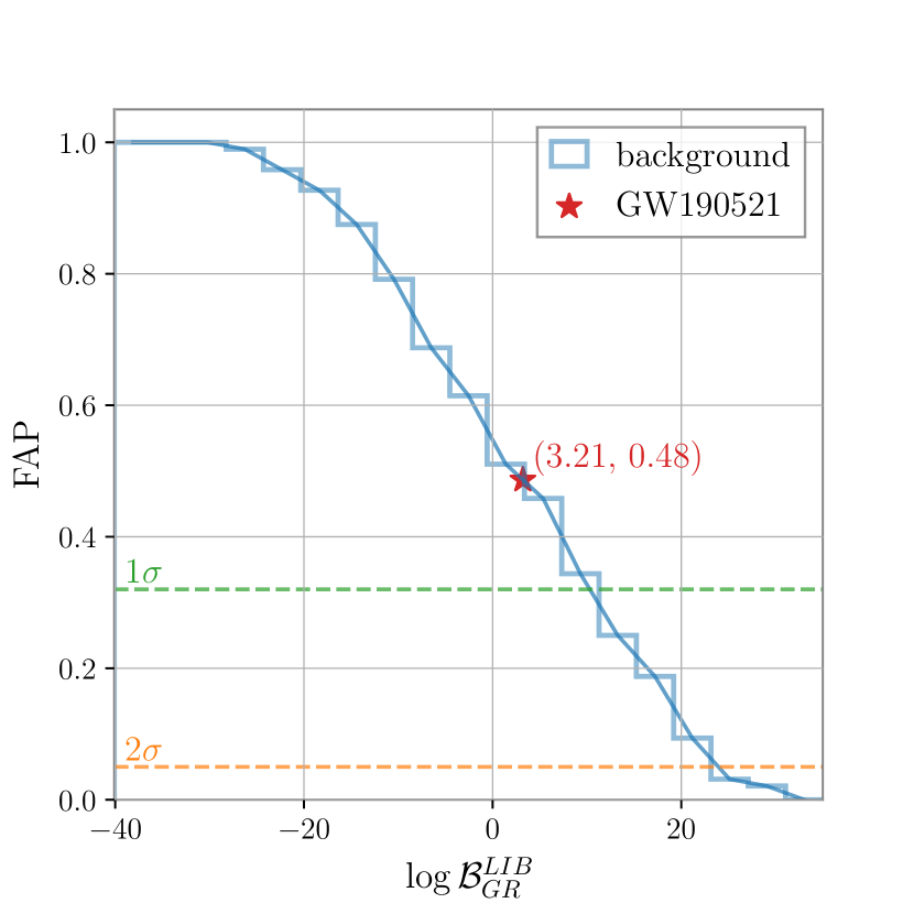
Figure 6: Bayes factors distributions for GW190521-like CBC, calculated by doing PE with both the hypothesis, for $\sim 100$ GR injections from the GW190521 posteriors in different realisations of gaussian noise. The false alarm probability for the observed $\log\mathcal{B}^{\text{LIB}}_{\text{GR}}=3.2$ is found to be $0.48$.

IV Implications

In our analysis of the latest GW catalog, we have found that the majority of the events disfavor birefringence. For a subset of them (most notably GW190521) while the Bayesian inference prefers the LIB hypothesis, a follow-up background study indicates that most simulated GR signals give comparable Bayes factors. In the following, we present the implications of these results. First, we consider the implications for generic LIB. Then, we study the constraints on a specific scalar-tensor theory that predicts LIB. Finally, we entertain the possibility that GW190521 was emitted in an active galactic nucleus (AGN) and is displaying evidence of birefringence.

IV.1 Constraints on generic LIB

From the non-observation of birefringence in the 43 events from GWTC-3 and using their median redshift values Abbott et al. (2021b), we estimate the total optical depth for the LIB models discussed in Sec. II.4. The non-observation of birefringence translates to constraints on the phenomenological model parameters, as summarized in Table 1. For reference, we also show the constraints obtained from the full GWTC-3 (90 events).

$\sigma_{\rm\text{LIB}}^{1/2}\hskip 5.69046pt$	95% c.l.	comment
$\propto M$	$R_{12}<4.4\,(2.9)$ kpc	Sec. IV.2
$\propto R_{E}$	$\alpha_{E}<3.0\,(1.6)$
$\propto M^{1/2}$	$R_{12}<20\,(12)$ kpc
$\propto M^{1/3}$	$R_{12}<12\,(6.9)$ kpc

Table 1: Constraints on the phenomenological models Eq. (14) and Eq. (15), assuming no birefringence detected for analysed (all) GWTC-3 events.

The higher redshift events have higher optical depth. Non-observation of birefringence in distant sources leads to more stringent constraints, although the SNR scales with the inverse luminosity distance: hence some of the highest redshift events will not be considered because of our FAR threshold. The final results depend strongly on the model via source redshift and halo mass function. Figure 7 shows the redshift dependence of the optical depth for the parameterizations discussed, adopting the 95% c.l. values found by our analysis along with the observed GWTC-3 redshift distribution.

Future observations will increase in number of events and their SNRs, allowing better constrain the birefringence probabilities and ruling out more of the parameter space in the alternative theories of gravity. Higher-redshift observations above our FAR threshold will be especially valuable to constrain $\alpha_{E}$ and $R_{12}$ for $n=1/3,1/2$ (see Fig. 7).

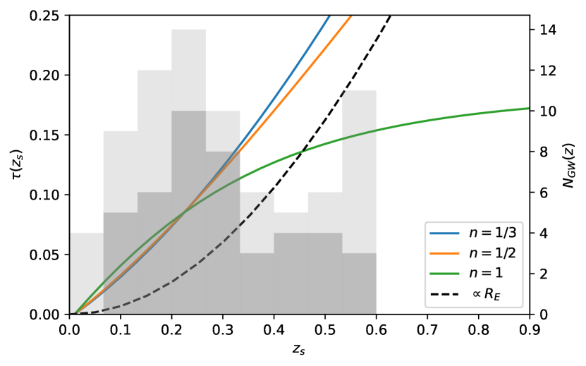
Figure 7: Birefringence optical depth for the phenomenological models considered here, using the parameters correspond to the 95% c.l. limit compatible with the non-observation of LIB. The dark (light) gray shaded histograms show the binned redshift distribution of analysed (all) GWTC-3 events. See Sec. II.4 for details.

IV.2 GW birefringence in Horndeski theories

Let us now use our results to a specific theory that predicts LIB. We will present the theory and translate the constraints of the phenomenological model (Table 1) into fundamental theory parameters. In the next subsection we will interpret a tentative detection of LIB in GW190521 as an AGN binary within the same theory. We will focus on a particular scalar-tensor theory within the Horndeski class Horndeski (1974), whose LIB predictions have been analyzed in detail, cf. Sec. 6 in Ref. Ezquiaga and Zumalacárregui (2020). The model is described by two parameters describing couplings between the Ricci scalar ($R$) and the new field $\phi$: a linear coupling $p_{4\phi}$ and a derivative coupling suppressed by an energy scale $\Lambda_{4}$. The Lagrangian of this theory can be written as Ezquiaga et al. (2016, 2017)

$$\mathcal{L}\sim-\frac{1}{2}(\nabla\phi)^{2}+\frac{M_{P}^{2}}{2}\left(1+\frac{p_{4\phi}\phi}{M_{P}}\right)R+\frac{\phi}{\Lambda_{4}^{2}}\nabla_{\mu}\nabla_{\nu}\phi G^{\mu\nu}\,,$$ (18)

where $R$ is the Ricci scalar, $G_{\mu\nu}$ is the Einstein tensor, $M_{P}$ is the Planck mass in units of $c=h=1$, and $\nabla$ the covariant derivative. The GR limit corresponds to $p_{4\phi}\to 0,\Lambda_{4}\to\infty$ . The parameters of this model are stringently constrained by the speed of GWs on the homogeneous FRW metric Ezquiaga and Zumalacárregui (2017); Creminelli and Vernizzi (2017); Baker et al. (2017); Sakstein and Jain (2017) (see also Brax et al. (2016); Lombriser and Taylor (2016); Bettoni et al. (2017)), as observed by the near-coincident arrival of GW170817 and its associated counterpart Abbott et al. (2017b): $|c_{g}/c-1|\lesssim 10^{-15}$. Compliance with this limit requires Ezquiaga and Zumalacárregui (2020)

$$p_{4\phi}\lesssim 10^{-8}\Lambda_{4}/H_{0}\quad\text{(GW170817)}\,.$$ (19)

While this constraint is extremely stringent, LIB allows comparable limits.

Specifying a model allows one to derive concrete predictions. The dependence of the time delay contributions (Shapiro, geometric) with the lens and theory parameters is complex. Nonetheless, we observed that the time delay decreases monotonically with the impact parameter. Moreover, its slope changes and becomes very sharp beyond the Vainshtein radius

$$r_{V}=1.2{\rm Mpc}\,p_{4\phi}^{1/3}\left(\frac{M}{10^{12}M_{\odot}}\right)^{1/3}\left(\frac{H_{0}}{\Lambda_{4}}\right)^{2/3}\,.$$ (20)

$r_{V}$ represents the scale at which the scalar field has a strong self-coupling near a massive object Vainshtein (1972). In many scalar-tensor theories this leads to screening: a suppression of scalar field fluctuations for $r<r_{V}$, allowing the theory to approximately recover GR around massive bodies. However, screening is not necessary in this model given the stringent constraint from GW170817 (Eq. (19)). In this case, the strong-interaction within $r_{V}$ represents a a large coupling between the scalar field and the Riemann tensor, the kind of interaction producing LIB.

For simplicity, we will focus on the Shapiro time delay. The geometric time delay is usually dominant for massive halos at intermediate distances. (Fig 12 in Ref. Ezquiaga and Zumalacárregui (2020)). It is proportional to the Einstein radius, and it could thus be captured generalizing Eq. 14 to extended lenses. Neglecting the geometric time delay is conservative but reasonable, since our constraints involve events at relatively low redshift ($z\lesssim 0.6$).

The LIB predictions have a simple dependence on the lens mass and theory parameters. We verified that $\Delta t_{12}\propto M\Lambda_{4}^{-4/3}$. The proportionality to the mass stems from the scaling with the Vainstein radius, as well as $\Delta t_{12}$, the impact parameter and the time spent by the GW on the region of sizeable birefringence are all $\propto r_{V}$. It allows us to directly connect the theory parameters to $R_{12}$ with $n=1$, as constrained in the phenomenological model (15). The scaling with $\Lambda_{4}$ allows us then to find $R_{12}$ by equating $\Delta t_{12}(R_{12})$ to the constrained value for different $p_{4\phi}$, but keeping $M=10^{12}M_{\odot}$, $\Lambda_{4}$ fixed. For simplicity, we will take a sensitivity of $\Delta t_{12}\sim 10$ ms to define $R_{12}$. Using the actual posteriors on $\Delta t_{12}$ for each of the GWTC-3 events analyzed will not qualitatively affect these constraints in any significant manner.

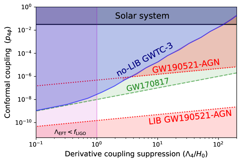
Figure 8: 95% c.l. constraints on the parameters of a quartic Horndeski theory Ezquiaga and Zumalacárregui (2020) using the lens-induced birrefringence (LIB) test. Shaded regions are excluded according to GWTC-3 (this work, blue solid), GW170817 Ezquiaga and Zumalacárregui (2017); Creminelli and Vernizzi (2017); Baker et al. (2017); Sakstein and Jain (2017) (green dashed) and GW190521 assuming an AGN binary  Graham et al. (2020) (red dotted, see Fig. 9). The GR limit corresponds to $p_{4\phi}\to 0,\Lambda_{4}\to\infty$, when the scalar field is decoupled from gravity and its derivative interactions suppressed. See sections IV.2, IV.3 for details. If GW190521 is associated to an AGN, the upper shaded region improves the overall GWTC-3 constraints for $\Lambda_{4}\gtrsim 3H_{0}$. If we further assume a detection of LIB, then the bottom red shaded region excludes GR. For reference, we also indicate Solar System constraints (gray horizontal) and the region there the GW frequencies at LIGO-Virgo detectors are larger than the (non-linear) energy scale of the effective field theory (magenta vertical).

The excluded region is shown in Fig. 8, along with constraints from the GW speed on FRW and lunar laser ranging (no screening, $p_{4\phi}\ll 1$, see Sec. VBc in Ref. Zumalacarregui (2020)). The change in slope at low $\Lambda$ corresponds to a transition in which $R_{12}$ surpasses the Vainsthein radius (20). For $\Lambda_{4}\ll H_{0}$ the birefringence constraints approach those of the GW speed: this happens when $r_{V}$ is so large that most GWs are effectively behind a lens. Then the constraints are satisfied in the limit $c_{\rm GW}\to c$, equivalent to Eq. (19). For the sensitivity of GWTC-3 this happens for $\Lambda_{4}\lesssim H_{0}$, where LVK frequencies lie beyond the validity of our framework as a classical effective field theory de Rham and Melville (2018). At increasing $\Lambda_{4}$ the constraints degrade, since probability becomes very suppressed, Eq. (20). For $\Lambda^{4}\gtrsim 10^{2}H_{0}$ solar system constraints become more efficient than birefringence.

IV.3 GW190521 as an AGN binary

Let us now discuss the implications of a possible birefringence detection associated to GW190521. Given the constraints from the speed of GWs (19) on our example Horndeski theory, the chances of birefringence being caused by a lens in the line of sight are very small. We will instead interpret our result, $\Delta t_{12}\gtrsim 9.5$ ms as due to an environmental effect near the source. We will follow the scenario outlined in Ref. Graham et al. (2020), where a candidate electromagnetic counterpart from an AGN J124942.3 + 344929, observed 34 days after the GW signal, suggests that the binary merged in the environment of a supermassive black hole (SMBH). Note that there are important uncertainties, both regarding the counterpart association (given large GW localization uncertainties Palmese et al. (2021)), and the significance of LIB detection (given our analysis of random noise realizations, Fig. 6). This discussion is therefore not a statement on the status of GR. Instead, it proves the potential of identifying environments of GW sources to test gravity theories.

Following Ref. Graham et al. (2020), we will assume an AGN binary scenario where the mass of the SMBH is $M_{\rm SMBH}\sim 10^{8}M_{\odot}$ and the source is located in a migration trap at $r\sim 700GM_{\rm SMBH}$. Then, using the framework of Ref. Ezquiaga and Zumalacárregui (2020) allows us to compute the time delay as a function of the angle between the observer and the source, relative to the SMBH. The results are shown in Fig. 9 for $p_{4\phi}=10^{-8},\Lambda_{4}=10H_{0}$, compatible GW170817 (19), and different distances to the SMBH (the dependence on $M_{\rm SMBH}$ is less pronounced, see below). The birefringent time delay becomes very large as $\theta\to 0$. Ultimately, the maximum time delay is limited by the existence of the horizon, $\theta_{s}\approx 2GM/r$. The birefringence also vanishes as $\theta\to\pi$ because of geometric cancellations in spherical symmetry.

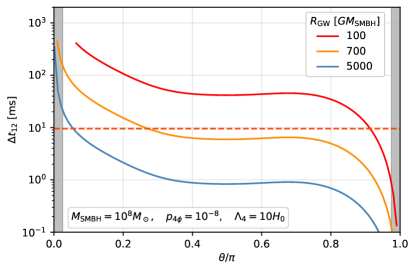
Figure 9: Birefringent time delay for a source near a SMBH as a function of the angle of the observer, relative to the SMBH. Each line corresponds to a different source distance, for model parameters compatible with GW170817 (see. Eq.  19). The horizontal line corresponds to the lower bound on $\Delta t_{12}=9.5$ ms from the analysis of GW190521. The region between the shaded areas encompasses 95% probability for a random observer. The lowest $\theta$ represents trajectories passing at 10 Schwarzschild radii of the SMBH.

We will translate these predictions into theory parameters and include the comparison to GW190521. We will take the values of $M_{\rm SMBH}$ and the source radius fixed, and consider the credible intervals as being determined by the angle $\theta$, cf. Eq. (21) and Appendix B. As we do not know the emission angle, we will assume a flat prior on the sphere $P(\theta)=\sin(\theta)$, and take the upper/lower 95% c.l. values based on $P(\theta)$ (excluding the shaded regions in Fig. 9). Limits on the theory parameters can be derived by noting that $\Delta t_{12}(\theta)\propto p_{4\phi}^{4/3}\Lambda_{4}^{-2/3}M_{\rm SMBH}^{1/3}$ including different assumptions about the SMBH mass. Note that $M_{\rm SMBH}$ enters with a different scaling than the lens mass in Sec. IV.2, due to the source being at a fixed distance from the SMBH and within its Vainsthein radius, rather than randomly located.

The implications of GW190521 for the example theory (18) are shown in Fig. 8. The orange regions are excluded if we assume the AGN scenario as discussed above. The lower region excludes the GR limit $p_{4\phi}\to 0,\Lambda_{4}\to\infty$ and relies on trusting the measured birefringence $\Delta t_{12}\gtrsim 9.5$ ms to be due to new gravitational physics. Even if the result is interpreted as noise (e.g. Fig. 6), assuming the AGN scenario leads to exclusion of the upper orange region (assuming sensitivity to $\Delta t_{12}\lesssim 9.5$ ms). Because of the different scaling with the theory parameters, the detection of an AGN binary becomes even more constraining than GW170817 for high $\Lambda_{4}$. The beyond GR interpretation can be further probed not only by AGN events but by high-redshift multi-messenger observations. In this case, the time delay between GWs and EM counterparts scales as $\approx 1s\left(10^{8}p_{4\phi}\frac{H_{0}}{\Lambda_{4}}\right)^{2}\frac{D}{40\rm Mpc}$ and can be probed by distant neutron-star mergers.

V Summary and Outlook

In this paper, we explored LIB as a test of GR using observations of GWs. LIB produces a difference in the arrival times of the GW polarisations in signals from the binary mergers, predicted by some alternatives to the GR. Using the Bayesian model selection framework, not only we can identify the signatures of birefringence, but also measure the time delay between the arrival of both polarisations ($\Delta t_{12}$). We show that this difference can be measured with high accuracy, of order few milliseconds with existing events and is likely to improve in the future following detector upgrades.

Using the latest GW catalog, GWTC-3, we find no strong evidence for the observation of the birefringence, with the highest $\log\mathcal{B}^{\text{LIB}}_{\text{GR}}=3.21$ for the heaviest binary black holes so far, GW190521. However, after simulating similar events under different noise realizations, we determine that there is a false alarm probability of 48%. This event has been associated with an AGN flare, possibly indicating that the merger occurred near a SMBH. This AGN scenario is especially favorable for the observation of LIB since the SMBH would act as a strong source of LIB. However, the AGN flare-GW association has been disputed, see e.g. Palmese et al. (2021). Moreover, the loudness and shortness of this event makes it susceptible to different astrophysical and fundamental physics interpretations. It has also been found to be violating many tests of GR and mimicking many exotic scenarios of compact binary such as head-on-collision of a boson star Calderón Bustillo et al. (2021) or left-right (L-R), frequency-dependent birefringence Wang et al. (2022). The latter effect is related to our flavour of LIB, with two important differences: first, L-R birefringence is defined in the basis of circularly polarized waves (left vs right, rather than $+$ vs $\times$), and second, it depends on the GW frequency. Both features also appear in the Gravitational spin Hall effect in GR, although the L-R time-delay is very suppressed Andersson et al. (2021); Oancea et al. (2022).

Of the 43 analyzed events, we find that the tightest bounds on the time delay between the two polarisations is $\Delta t_{12}\sim 0.51$ ms at 90% credible intervals coming from the GW$200311\_115853$ merger event, while the median is $\Delta t_{12}\simeq 80$ ms. From the non-observation of LIB, we constrained the lensing optical depths in a phenomenological parameterization in which the lensing cross-section is proportional to the Einstein radius or a fixed physical radius with a power law scaling in the halo mass.

Our constraints can be translated to gravitational theories that predict LIB. As an example, we presented novel constraints on a Horndeski scalar-tensor theory featuring a new dynamical field and two free parameters. The theory is stringently constrained by the speed of GWs on the homogeneous FRW background following GW170817. Nevertheless, the lack of observed LIB places stringent bounds, which can be orders of magnitude better than Solar System tests and in some limits as tight as the GW speed bound. As a proof of principle of LIB due to a known inhomogeneity, we interpret GW190521 as an AGN binary (assuming that the signal originated in close proximity to a SMBH Graham et al. (2020)) in terms of our example theory. Then, the large curvature is able to generate detectable LIB even when deviations from GR are minute. Our $|\Delta t_{12}|\gtrsim 9.5$ ms results would then exclude GR, placing a minimum value of the theory parameters. When interpreting this result as a fluctuation and GR to be correct, the AGN hypothesis is still able to produce very stringent bounds, that can even overcome those of the GW speed on FRW.

In future, the methods we developed here can be useful for studying new classes of events. Of particular interest will be signals where the merger is either near an SMBH or is known to have a lensed counterpart due to strong lensing. In such cases, the information about the lens may improve the constraints substantially, along the lines of the AGN-scenario we discussed. The increase in detection rate and a growing chance of strongly lensed GW identification makes LIB test also relevant for future runs of LVK detectors and upcoming GW detectors such as Einstein Telescope, Cosmic Explorer and LISA Kalogera et al. (2021); Sathyaprakash et al. (2012); Ding et al. (2015); Çalışkan et al. (2022). Lastly, the addition of ground-based detectors such as LIGO-India and KAGRA can allow us to measure extra linear combinations of the GW polarisations and construct a null-stream Chatziioannou et al. (2012) to extract each of the polarisations individually. The extracted polarisations can then be used to test their consistency with GR or other theories of gravity directly.

Strongly lensed GW signals may allow us to measure additional linear combinations of the same GW polarisations and hence improve various tests of GR  Goyal et al. (2021), including the one proposed here. Ultimately, developing LIB predictions for other alternative theories and generalizing the model-independent parameterizations presented here will allow our results to further test the landscape of theories beyond GR.

VI Acknowledgements

We are grateful to A. K. Mehta, P. Ajith, G. Brando, S. Savastano, G. Tambalo, Y. Wang, H. Villarrubia-Rojo and J. Tasson for fruitful discussions. SG and AV are supported by the Department of Atomic Energy, Government of India, under Project No. RTI4001. AV is also supported by a Fulbright Program grant under the Fulbright-Nehru Doctoral Research Fellowship, sponsored by the Bureau of Educational and Cultural Affairs of the United States Department of State and administered by the Institute of International Education and the United States-India Educational Foundation. J.M.E. is supported by the European Union’s Horizon 2020 research and innovation program under the Marie Sklodowska-Curie grant agreement No. 847523 INTERACTIONS, by VILLUM FONDEN (grant no. 37766), by the Danish Research Foundation, and under the European Union’s H2020 ERC Advanced Grant “Black holes: gravitational engines of discovery” grant agreement no. Gravitas–101052587. The numerical calculations reported in the paper are performed on the Alice computing cluster at ICTS-TIFR, with the aid of LALSuite LIGO Scientific Collaboration (2018), Bilby Ashton et al. (2019), PyCBC Nitz et al. (2020b) and Colossus Diemer (2018) software packages. This material is based upon work supported by NSF’s LIGO Laboratory which is a major facility fully funded by the National Science Foundation.

Appendix A Injection Parameters

Here we list the injection parameters for the mismatch and the parameter estimation studies. Note that the luminosity distances are scaled as per the SNRs and hence are not mentioned in the table below.

$m_{1}$	$m_{2}$	$\delta$	$\alpha$	$\iota$	$\chi_{1}$	$\chi_{2}$	$\psi$	$\phi_{c}$	$t_{c}$
$38.3$	$33.19$	$-1.2$	$2.3$	$2.9$	$0.3$	$0.27$	$1.6$	$1.9$	$1126259462.414$
$24.4$	$2.7$	$-0.4$	$0.2$	$0.5$	$0.06$	$0.46$	$1.5$	$4.4$	$1249852256.99$

Table 2: GW150914-like (top) and GW190814-like (bottom) CBC parameters used during mismatch calculations in Sec. II.2 and PE injection studies in Sec. III.

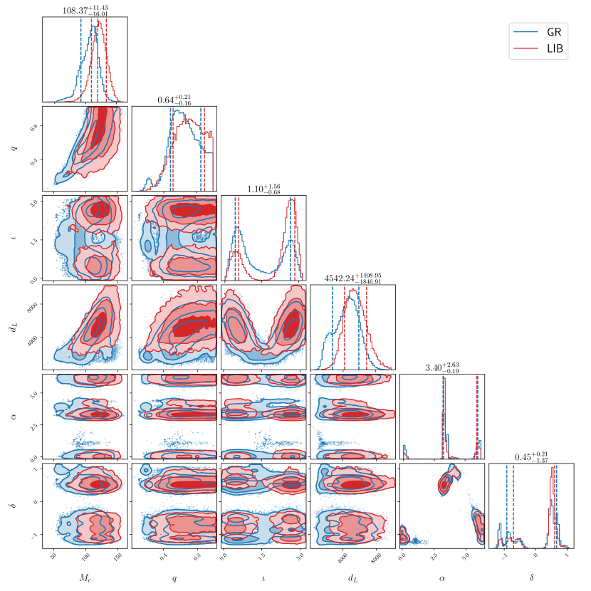
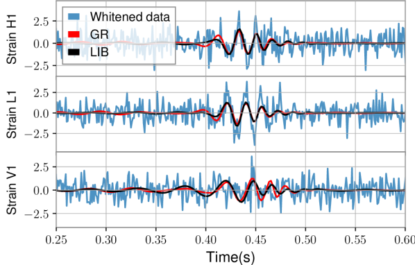
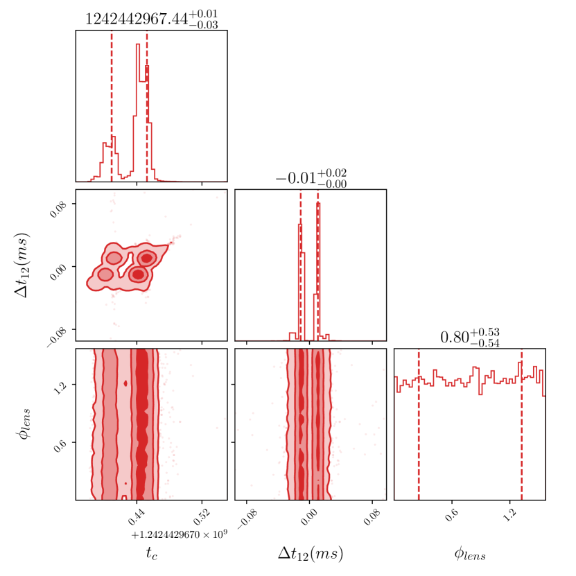
Figure 10: $GW190521$($\log\mathcal{B}^{\text{LIB}}_{\text{GR}}=3.21$) GR v/s LIB posteriors. $MaP$ (maximum a posteriori) waveforms under GR and LIB ($\Delta t_{12}=9.51\mathrm{ms},\phi_{\mathrm{lens}}=0.06\mathrm{rad}$) hypothesis with the whitened strain as observed at the LIGO-Virgo detectors.

Appendix B Beyond-Poisson statistics

The independent lens assumption fails to capture two circumstances that potentially enhance the detection of birefringence: the source environment and lensing by known objects. This situation is qualitatively different from strong lensing probabilities, which are weighted by the Einstein radius, which vanishes when $D_{L}\to D_{S}$ (near the source) or $D_{L}\to 0$ (near the detector). In contrast, birefringence probabilities do not suffer such suppression and can be sizeable for objects near the source or the observer. Our optical-depth framework (Sec. II.4) does not consider this possibility.

Source environment may play a role for LIB, as GW sources will generally be located in regions denser than the cosmic average. In this case, the host galaxy (or objects within it) would have a much larger density compared to the cosmological average used in, e.g. Eq. (16). In addition, the projected cross-section $\propto 1/D^{2}$ will be larger for nearby objects, thus enhancing the probabilities. Given a distribution of GW sources near an object, the posterior on the theory parameters $\vec{p}$ can be obtained as

$$P(\vec{p})=\int drd\theta P_{\rm s}(r)\sin(\theta)P\left(\Delta t_{12}(r,\theta,\vec{p})\right)\,.$$ (21)

Here we have assumed a symmetric $r$-dependent distribution. The $\theta$ dependence corresponds to a uniform prior on the sphere. This simple dependence could be used to model the effect of the source’s galaxy or nearby objects.

An extreme case of environmental enhancement is given by a binary merging in an AGN near a supermassive black hole (SMBH), as discussed in Sec. IV.3, taking the multi-messenger scenario of GW190521 and its implications for the example Horndeski theory. Estimates for the rate of such events are uncertain. Nonetheless, in some cases it might be possible to associate an event with a SMBH thanks to an EM counterpart Graham et al. (2020), multiple images due to strong lensing O’Leary et al. (2009); Kocsis and Levin (2012); D’Orazio and Loeb (2020) or strong-field propagation effects Oancea et al. (2022).

Another potential to improve the quoted result is by correlating GW arrival direction with known lenses. relevant in cases where the Milky Way (or perhaps even the Sun) may imprint an observable birefringence. Adding information on the GW direction, relative to known objects, will allow better constraints on those scenarios more effectively than assuming randomly located lenses. For instance, if stellar-scale lenses are relevant in a given theory and the cross-section scales as the physical radius (allowing nearby lenses to contribute), sources behind the milky way can probe a much larger effective cross-section than given by Eq. 17.

Finally, any confident detection of a lensed GW can be used to refine constraints within a given model. This would follow either through the identification of several GW detections as images of the same underlying source or through waveform distortions (millilensing). Both cases allow information about the lens mass and impact parameter to be recovered, at least when assuming a lens model Takahashi and Nakamura (2003); Çalışkan et al. (2022); Tambalo et al. (2022). That information can then place constraints within a specific theory of gravity.

Appendix C GW190521 posteriors under LIB and GR

In Fig. 10 we show the posteriors of the GW190521 event which has the highest log Bayes factor ($\ln\mathcal{B}^{\text{LIB}}_{\text{GR}}=3.21$) from the PE runs of LIB and GR hypothesis. The two posteriors are consistent with each other with LIB favouring a slightly higher luminosity distance ($d_{L}$) and chirp mass ($M_{c}$). Additionally, posteriors under LIB are marginally narrower as compared to GR, which might be a reason for its $\ln\mathcal{B}^{\text{LIB}}_{\text{GR}}>0$. It is worth noticing that $\Delta t_{12}$ is degenerate with $t_{c}$, which is itself poorly measured due to low SNR in Virgo. We also plot the waveforms using maximum a posteriori (MaP) parameters along with the whitened time series data Abbott et al. (2020) as observed in the Hanford (H1), Livingston (L1) and Virgo (V1) detectors. It’s easy to see that the signal duration is small and the two MaP waveforms are not very different from each other except for the tiny modulations in the LIB one. It can thus be concluded that the model selection favours the LIB hypothesis because it is fitting better the random noise at the detectors during the event GW190521.

References

- Aasi et al. (2015) J. Aasi et al. (LIGO Scientific), “Advanced LIGO,” Class. Quant. Grav. 32, 074001 (2015), arXiv:1411.4547 [gr-qc] .
- Acernese et al. (2015) F. Acernese et al. (Virgo), “Advanced Virgo: a second-generation interferometric gravitational wave detector,” Class. Quant. Grav. 32, 024001 (2015), arXiv:1408.3978 [gr-qc] .
- Aso et al. (2013) Yoichi Aso, Yuta Michimura, Kentaro Somiya, Masaki Ando, Osamu Miyakawa, Takanori Sekiguchi, Daisuke Tatsumi, and Hiroaki Yamamoto (KAGRA), “Interferometer design of the KAGRA gravitational wave detector,” Phys. Rev. D88, 043007 (2013), arXiv:1306.6747 [gr-qc] .
- Abbott et al. (2016) B. P. Abbott et al. (LIGO Scientific Collaboration and Virgo Collaboration), “Observation of gravitational waves from a binary black hole merger,” Phys. Rev. Lett. 116, 061102 (2016).
- Abbott et al. (2017a) B.?P. Abbott et al. (Virgo, LIGO Scientific), “GW170817: Observation of Gravitational Waves from a Binary Neutron Star Inspiral,” Phys. Rev. Lett. 119, 161101 (2017a), arXiv:1710.05832 [gr-qc] .
- Abbott et al. (2019a) B. P. Abbott et al. (LIGO Scientific, Virgo), “GWTC-1: A Gravitational-Wave Transient Catalog of Compact Binary Mergers Observed by LIGO and Virgo during the First and Second Observing Runs,” Phys. Rev. X9, 031040 (2019a), arXiv:1811.12907 [astro-ph.HE] .
- Abbott et al. (2021a) R. Abbott et al. (LIGO Scientific, Virgo), “GWTC-2: Compact Binary Coalescences Observed by LIGO and Virgo During the First Half of the Third Observing Run,” Phys. Rev. X 11, 021053 (2021a), arXiv:2010.14527 [gr-qc] .
- Abbott et al. (2021b) R. Abbott et al. (LIGO Scientific, Virgo, KAGRA), “GWTC-3: Compact Binary Coalescences Observed by LIGO and Virgo During the Second Part of the Third Observing Run,” (2021b), arXiv:2111.03606 [gr-qc] .
- Nitz et al. (2020a) Alexander H. Nitz, Thomas Dent, Gareth S. Davies, Sumit Kumar, Collin D. Capano, Ian Harry, Simone Mozzon, Laura Nuttall, Andrew Lundgren, and Márton Tápai, “2-OGC: Open Gravitational-wave Catalog of binary mergers from analysis of public Advanced LIGO and Virgo data,” Astrophys. J. 891, 123 (2020a), arXiv:1910.05331 [astro-ph.HE] .
- Nitz et al. (2021) Alexander H. Nitz, Sumit Kumar, Yi-Fan Wang, Shilpa Kastha, Shichao Wu, Marlin Schäfer, Rahul Dhurkunde, and Collin D. Capano, “4-OGC: Catalog of gravitational waves from compact-binary mergers,” (2021), arXiv:2112.06878 [astro-ph.HE] .
- Venumadhav et al. (2020) Tejaswi Venumadhav, Barak Zackay, Javier Roulet, Liang Dai, and Matias Zaldarriaga, “New binary black hole mergers in the second observing run of Advanced LIGO and Advanced Virgo,” Phys. Rev. D 101, 083030 (2020), arXiv:1904.07214 [astro-ph.HE] .
- Abbott et al. (2016) B. P. Abbott et al. (LIGO Scientific and Virgo Collaborations), “Tests of general relativity with gw150914,” Phys. Rev. Lett. 116, 221101 (2016).
- Abbott et al. (2019b) B.P. Abbott et al. (LIGO Scientific, Virgo), “Tests of General Relativity with the Binary Black Hole Signals from the LIGO-Virgo Catalog GWTC-1,” Phys. Rev. D 100, 104036 (2019b), arXiv:1903.04467 [gr-qc] .
- Abbott et al. (2021c) R. Abbott et al. (LIGO Scientific, Virgo), “Tests of general relativity with binary black holes from the second LIGO-Virgo gravitational-wave transient catalog,” Phys. Rev. D 103, 122002 (2021c), arXiv:2010.14529 [gr-qc] .
- Abbott et al. (2021d) R. Abbott et al. (LIGO Scientific, Virgo, KAGRA), “Tests of General Relativity with GWTC-3,” (2021d), arXiv:2112.06861 [gr-qc] .
- Will (1998) Clifford M. Will, “Bounding the mass of the graviton using gravitational wave observations of inspiralling compact binaries,” Phys. Rev. D57, 2061–2068 (1998), arXiv:gr-qc/9709011 [gr-qc] .
- Ezquiaga and Zumalacárregui (2018) Jose María Ezquiaga and Miguel Zumalacárregui, “Dark Energy in light of Multi-Messenger Gravitational-Wave astronomy,” Front. Astron. Space Sci. 5, 44 (2018), arXiv:1807.09241 [astro-ph.CO] .
- Arai and Nishizawa (2018) Shun Arai and Atsushi Nishizawa, “Generalized framework for testing gravity with gravitational-wave propagation. ii. constraints on horndeski theory,” Phys. Rev. D 97, 104038 (2018).
- Nishizawa (2018) Atsushi Nishizawa, “Generalized framework for testing gravity with gravitational-wave propagation. i. formulation,” Physical Review D 97 (2018), 10.1103/physrevd.97.104037.
- Will (2014) Clifford M. Will, “The Confrontation between General Relativity and Experiment,” Living Rev. Rel. 17, 4 (2014), arXiv:1403.7377 [gr-qc] .
- Workman and Others (2022) R. L. Workman and Others (Particle Data Group), “Review of Particle Physics,” PTEP 2022, 083C01 (2022).
- Max et al. (2017) Kevin Max, Moritz Platscher, and Juri Smirnov, “Gravitational Wave Oscillations in Bigravity,” Phys. Rev. Lett. 119, 111101 (2017), arXiv:1703.07785 [gr-qc] .
- Max et al. (2018) Kevin Max, Moritz Platscher, and Juri Smirnov, “Decoherence of Gravitational Wave Oscillations in Bigravity,” Phys. Rev. D97, 064009 (2018), arXiv:1712.06601 [gr-qc] .
- Belgacem et al. (2019) Enis Belgacem et al. (LISA Cosmology Working Group), “Testing modified gravity at cosmological distances with LISA standard sirens,” JCAP 07, 024 (2019), arXiv:1906.01593 [astro-ph.CO] .
- Jiménez et al. (2020) Jose Beltrán Jiménez, Jose María Ezquiaga, and Lavinia Heisenberg, “Probing cosmological fields with gravitational wave oscillations,” JCAP 04, 027 (2020), arXiv:1912.06104 [astro-ph.CO] .
- Ezquiaga et al. (2021a) Jose Maria Ezquiaga, Wayne Hu, Macarena Lagos, and Meng-Xiang Lin, “Gravitational wave propagation beyond general relativity: waveform distortions and echoes,” JCAP 11, 048 (2021a), arXiv:2108.10872 [astro-ph.CO] .
- Ezquiaga and Zumalacárregui (2020) Jose María Ezquiaga and Miguel Zumalacárregui, “Gravitational wave lensing beyond general relativity: birefringence, echoes and shadows,” Phys. Rev. D 102, 124048 (2020), arXiv:2009.12187 [gr-qc] .
- Dalang et al. (2021) Charles Dalang, Pierre Fleury, and Lucas Lombriser, “Scalar and tensor gravitational waves,” Phys. Rev. D 103, 064075 (2021), arXiv:2009.11827 [gr-qc] .
- Okounkova et al. (2022) Maria Okounkova, Will M. Farr, Maximiliano Isi, and Leo C. Stein, “Constraining gravitational wave amplitude birefringence and Chern-Simons gravity with GWTC-2,” Phys. Rev. D 106, 044067 (2022), arXiv:2101.11153 [gr-qc] .
- Vitale et al. (2022) Salvatore Vitale, Sylvia Biscoveanu, and Colm Talbot, “The orientations of the binary black holes in GWTC-3,” (2022), arXiv:2204.00968 [gr-qc] .
- de Rham and Tolley (2020) Claudia de Rham and Andrew J. Tolley, “Speed of gravity,” Phys. Rev. D 101, 063518 (2020), arXiv:1909.00881 [hep-th] .
- Andersson et al. (2021) Lars Andersson, Jérémie Joudioux, Marius A. Oancea, and Ayush Raj, “Propagation of polarized gravitational waves,” Phys. Rev. D 103, 044053 (2021), arXiv:2012.08363 [gr-qc] .
- Oancea et al. (2022) Marius A. Oancea, Richard Stiskalek, and Miguel Zumalacárregui, “From the gates of the abyss: Frequency- and polarization-dependent lensing of gravitational waves in strong gravitational fields,” (2022), arXiv:2209.06459 [gr-qc] .
- Wang et al. (2022) Yi-Fan Wang, Stephanie M. Brown, Lijing Shao, and Wen Zhao, “Tests of gravitational-wave birefringence with the open gravitational-wave catalog,” Phys. Rev. D 106, 084005 (2022), arXiv:2109.09718 [astro-ph.HE] .
- Haegel et al. (2022) Leïla Haegel, Kellie O’Neal-Ault, Quentin G. Bailey, Jay D. Tasson, Malachy Bloom, and Lijing Shao, “Search for anisotropic, birefringent spacetime-symmetry breaking in gravitational wave propagation from GWTC-3,” (2022), arXiv:2210.04481 [gr-qc] .
- Bombacigno et al. (2022) Flavio Bombacigno, Fabio Moretti, Simon Boudet, and Gonzalo J. Olmo, “Landau damping for gravitational waves in parity-violating theories,” (2022), arXiv:2210.07673 [gr-qc] .
- Veitch et al. (2015) J. Veitch et al., “Parameter estimation for compact binaries with ground-based gravitational-wave observations using the LALInference software library,” Phys. Rev. D91, 042003 (2015), arXiv:1409.7215 [gr-qc] .
- Ezquiaga et al. (2021b) Jose María Ezquiaga, Daniel E. Holz, Wayne Hu, Macarena Lagos, and Robert M. Wald, “Phase effects from strong gravitational lensing of gravitational waves,” Phys. Rev. D 103, 064047 (2021b), arXiv:2008.12814 [gr-qc] .
- Cusin and Lagos (2020) Giulia Cusin and Macarena Lagos, “Gravitational wave propagation beyond geometric optics,” Phys. Rev. D 101, 044041 (2020), arXiv:1910.13326 [gr-qc] .
- Pratten et al. (2021) Geraint Pratten, Cecilio García-Quirós, Marta Colleoni, Antoni Ramos-Buades, Héctor Estellés, Maite Mateu-Lucena, Rafel Jaume, Maria Haney, David Keitel, Jonathan E. Thompson, and Sascha Husa, “Computationally efficient models for the dominant and subdominant harmonic modes of precessing binary black holes,” Phys. Rev. D 103, 104056 (2021), arXiv:2004.06503 [gr-qc] .
- LIGO Scientific Collaboration (2018) LIGO Scientific Collaboration, “LIGO Algorithm Library - LALSuite,” free software (GPL) (2018).
- Ashton et al. (2019) Gregory Ashton, Moritz Hübner, Paul D. Lasky, Colm Talbot, Kendall Ackley, Sylvia Biscoveanu, Qi Chu, Atul Divakarla, Paul J. Easter, Boris Goncharov, Francisco Hernandez Vivanco, Jan Harms, Marcus E. Lower, Grant D. Meadors, Denyz Melchor, Ethan Payne, Matthew D. Pitkin, Jade Powell, Nikhil Sarin, Rory J. E. Smith, and Eric Thrane, “BILBY: A User-friendly Bayesian Inference Library for Gravitational-wave Astronomy,” Apjs 241, 27 (2019), 1811.02042 [astro-ph.IM] .
- Nitz et al. (2020b) Alex Nitz et al., “gwastro/pycbc: Pycbc release v1.16.8,” (2020b).
- The Virgo Collaboration (2012) The Virgo Collaboration, Advanced Virgo sensitivity curve study, Tech. Rep. VIR-0073D-12 (Virgo Collaboration, 2012).
- aLI (2018) The updated Advanced LIGO design curve, Tech. Rep. LIGO-T1800044-v5 (LIGO Document Control Center, 2018).
- Skilling (2006) John Skilling, “Nested sampling for general bayesian computation,” Bayesian Anal. 1, 833–859 (2006).
- Speagle (2020) Joshua S. Speagle, “dynesty: a dynamic nested sampling package for estimating Bayesian posteriors and evidences,” Mon. Not. Roy. Astron. Soc. 493, 3132–3158 (2020), arXiv:1904.02180 [astro-ph.IM] .
- Vitale et al. (2020) Salvatore Vitale, Davide Gerosa, Will M. Farr, and Stephen R. Taylor, “Inferring the properties of a population of compact binaries in presence of selection effects,” (2020), arXiv:2007.05579 [astro-ph.IM] .
- Xu et al. (2022) Fei Xu, Jose Marí a Ezquiaga, and Daniel E. Holz, “Please repeat: Strong lensing of gravitational waves as a probe of compact binary and galaxy populations,” The Astrophysical Journal 929, 9 (2022).
- Pei (1993) Y. Pei, “Probability of lensing magnification by cosmologically-distributed point masses.” Frontiers of Astronomy in 1990s. Proc. Workshop held in Beijing , 88–93 (1993).
- Zumalacarregui and Seljak (2018) Miguel Zumalacarregui and Uros Seljak, “Limits on stellar-mass compact objects as dark matter from gravitational lensing of type Ia supernovae,” Phys. Rev. Lett. 121, 141101 (2018), arXiv:1712.02240 [astro-ph.CO] .
- Tinker et al. (2008) Jeremy L. Tinker, Andrey V. Kravtsov, Anatoly Klypin, Kevork Abazajian, Michael S. Warren, Gustavo Yepes, Stefan Gottlober, and Daniel E. Holz, “Toward a halo mass function for precision cosmology: The Limits of universality,” Astrophys. J. 688, 709–728 (2008), arXiv:0803.2706 [astro-ph] .
- Diemer (2018) Benedikt Diemer, “COLOSSUS: A python toolkit for cosmology, large-scale structure, and dark matter halos,” Astrophys. J. Suppl. 239, 35 (2018), arXiv:1712.04512 [astro-ph.CO] .
- Aghanim et al. (2020) N. Aghanim et al. (Planck), “Planck 2018 results. VI. Cosmological parameters,” Astron. Astrophys. 641, A6 (2020), [Erratum: Astron.Astrophys. 652, C4 (2021)], arXiv:1807.06209 [astro-ph.CO] .
- Zumalacarregui (2020) Miguel Zumalacarregui, “Gravity in the Era of Equality: Towards solutions to the Hubble problem without fine-tuned initial conditions,” Phys. Rev. D 102, 023523 (2020), arXiv:2003.06396 [astro-ph.CO] .
- Alonso et al. (2017) David Alonso, Emilio Bellini, Pedro G. Ferreira, and Miguel Zumalacárregui, “Observational future of cosmological scalar-tensor theories,” Phys. Rev. D95, 063502 (2017), arXiv:1610.09290 [astro-ph.CO] .
- Vainshtein (1972) A. I. Vainshtein, “To the problem of nonvanishing gravitation mass,” Phys. Lett. B39, 393–394 (1972).
- Calderón Bustillo et al. (2021) Juan Calderón Bustillo, Nicolas Sanchis-Gual, Alejandro Torres-Forné, José A. Font, Avi Vajpeyi, Rory Smith, Carlos Herdeiro, Eugen Radu, and Samson H. W. Leong, “GW190521 as a Merger of Proca Stars: A Potential New Vector Boson of eV,” Phys. Rev. Lett. 126, 081101 (2021), arXiv:2009.05376 [gr-qc] .
- Horndeski (1974) Gregory Walter Horndeski, “Second-order scalar-tensor field equations in a four-dimensional space,” Int. J. Theor. Phys. 10, 363–384 (1974).
- Ezquiaga et al. (2016) Jose María Ezquiaga, Juan García-Bellido, and Miguel Zumalacárregui, “Towards the most general scalar-tensor theories of gravity: a unified approach in the language of differential forms,” Phys. Rev. D94, 024005 (2016), arXiv:1603.01269 [hep-th] .
- Ezquiaga et al. (2017) Jose María Ezquiaga, Juan García-Bellido, and Miguel Zumalacárregui, “Field redefinitions in theories beyond Einstein gravity using the language of differential forms,” Phys. Rev. D95, 084039 (2017), arXiv:1701.05476 [hep-th] .
- Ezquiaga and Zumalacárregui (2017) Jose María Ezquiaga and Miguel Zumalacárregui, “Dark Energy After GW170817: Dead Ends and the Road Ahead,” Phys. Rev. Lett. 119, 251304 (2017), arXiv:1710.05901 [astro-ph.CO] .
- Creminelli and Vernizzi (2017) Paolo Creminelli and Filippo Vernizzi, “Dark Energy after GW170817 and GRB170817A,” Phys. Rev. Lett. 119, 251302 (2017), arXiv:1710.05877 [astro-ph.CO] .
- Baker et al. (2017) T. Baker, E. Bellini, P. G. Ferreira, M. Lagos, J. Noller, and I. Sawicki, “Strong constraints on cosmological gravity from GW170817 and GRB 170817A,” Phys. Rev. Lett. 119, 251301 (2017), arXiv:1710.06394 [astro-ph.CO] .
- Sakstein and Jain (2017) Jeremy Sakstein and Bhuvnesh Jain, “Implications of the Neutron Star Merger GW170817 for Cosmological Scalar-Tensor Theories,” Phys. Rev. Lett. 119, 251303 (2017), arXiv:1710.05893 [astro-ph.CO] .
- Brax et al. (2016) Philippe Brax, Clare Burrage, and Anne-Christine Davis, “The Speed of Galileon Gravity,” JCAP 1603, 004 (2016), arXiv:1510.03701 [gr-qc] .
- Lombriser and Taylor (2016) Lucas Lombriser and Andy Taylor, “Breaking a Dark Degeneracy with Gravitational Waves,” JCAP 1603, 031 (2016), arXiv:1509.08458 [astro-ph.CO] .
- Bettoni et al. (2017) Dario Bettoni, Jose María Ezquiaga, Kurt Hinterbichler, and Miguel Zumalacárregui, “Speed of Gravitational Waves and the Fate of Scalar-Tensor Gravity,” Phys. Rev. D95, 084029 (2017), arXiv:1608.01982 [gr-qc] .
- Abbott et al. (2017b) B. P. Abbott et al. (Virgo, Fermi-GBM, INTEGRAL, LIGO Scientific), “Gravitational Waves and Gamma-rays from a Binary Neutron Star Merger: GW170817 and GRB 170817A,” Astrophys. J. 848, L13 (2017b), arXiv:1710.05834 [astro-ph.HE] .
- Graham et al. (2020) M. J. Graham et al., “Candidate Electromagnetic Counterpart to the Binary Black Hole Merger Gravitational Wave Event S190521g,” Phys. Rev. Lett. 124, 251102 (2020), arXiv:2006.14122 [astro-ph.HE] .
- de Rham and Melville (2018) Claudia de Rham and Scott Melville, “Gravitational Rainbows: LIGO and Dark Energy at its Cutoff,” Phys. Rev. Lett. 121, 221101 (2018), arXiv:1806.09417 [hep-th] .
- Palmese et al. (2021) Antonella Palmese, Maya Fishbach, Colin J. Burke, James T. Annis, and Xin Liu, “Do LIGO/Virgo Black Hole Mergers Produce AGN Flares? The Case of GW190521 and Prospects for Reaching a Confident Association,” Astrophys. J. Lett. 914, L34 (2021), arXiv:2103.16069 [astro-ph.HE] .
- Kalogera et al. (2021) Vicky Kalogera et al., “The Next Generation Global Gravitational Wave Observatory: The Science Book,” (2021), arXiv:2111.06990 [gr-qc] .
- Sathyaprakash et al. (2012) B. Sathyaprakash et al., “Scientific Objectives of Einstein Telescope,” Gravitational waves. Numerical relativity - data analysis. Proceedings, 9th Edoardo Amaldi Conference, Amaldi 9, and meeting, NRDA 2011, Cardiff, UK, July 10-15, 2011, Class. Quant. Grav. 29, 124013 (2012), [Erratum: Class. Quant. Grav.30,079501(2013)], arXiv:1206.0331 [gr-qc] .
- Ding et al. (2015) Xuheng Ding, Marek Biesiada, and Zong-Hong Zhu, “Strongly lensed gravitational waves from intrinsically faint double compact binaries—prediction for the Einstein Telescope,” JCAP 12, 006 (2015), arXiv:1508.05000 [astro-ph.HE] .
- Çalışkan et al. (2022) Mesut Çalışkan, Lingyuan Ji, Roberto Cotesta, Emanuele Berti, Marc Kamionkowski, and Sylvain Marsat, “Observability of lensing of gravitational waves from massive black hole binaries with lisa,” (2022).
- Chatziioannou et al. (2012) Katerina Chatziioannou, Nicolas Yunes, and Neil Cornish, “Model-Independent Test of General Relativity: An Extended post-Einsteinian Framework with Complete Polarization Content,” Phys. Rev. D86, 022004 (2012), [Erratum: Phys. Rev.D95,no.12,129901(2017)], arXiv:1204.2585 [gr-qc] .
- Goyal et al. (2021) Srashti Goyal, K. Haris, Ajit Kumar Mehta, and Parameswaran Ajith, “Testing the nature of gravitational-wave polarizations using strongly lensed signals,” Physical Review D 103 (2021), 10.1103/physrevd.103.024038.
- O’Leary et al. (2009) Ryan M. O’Leary, Bence Kocsis, and Abraham Loeb, “Gravitational waves from scattering of stellar-mass black holes in galactic nuclei,” Mon. Not. Roy. Astron. Soc. 395, 2127–2146 (2009), arXiv:0807.2638 [astro-ph] .
- Kocsis and Levin (2012) Bence Kocsis and Janna Levin, “Repeated Bursts from Relativistic Scattering of Compact Objects in Galactic Nuclei,” Phys. Rev. D 85, 123005 (2012), arXiv:1109.4170 [astro-ph.CO] .
- D’Orazio and Loeb (2020) Daniel J. D’Orazio and Abraham Loeb, “Repeated gravitational lensing of gravitational waves in hierarchical black hole triples,” Phys. Rev. D 101, 083031 (2020), arXiv:1910.02966 [astro-ph.HE] .
- Takahashi and Nakamura (2003) Ryuichi Takahashi and Takashi Nakamura, “Wave effects in gravitational lensing of gravitational waves from chirping binaries,” Astrophys. J. 595, 1039–1051 (2003), arXiv:astro-ph/0305055 .
- Tambalo et al. (2022) Giovanni Tambalo, Miguel Zumalacárregui, Liang Dai, and Mark Ho-Yeuk Cheung, “Gravitational wave lensing as a probe of halo properties and dark matter,” (2022), arXiv:2212.11960 [astro-ph.CO] .
- Abbott et al. (2020) R. Abbott et al. (LIGO Scientific, Virgo), “GW190521: A Binary Black Hole Merger with a Total Mass of ,” Phys. Rev. Lett. 125, 101102 (2020), arXiv:2009.01075 [gr-qc] .