First-principles thermal equation of state of fcc iridium

Abstract

The thermal equation of states for fcc iridium (Ir) is obtained from first-principles molecular dynamics up to 3000 K and 540 GPa. The equation of state (EoS) is globally fitted to a simplified free energy model and various parameters are derived. The theoretical principal Hugoniot is compared with shockwave experiments, where discrepancy suggests formation of new Ir phases. A few representative EoS parameters, such as bulk modulus $K_{T}$, thermal expansivity $\alpha$, Grüneisen parameter $\gamma$, and constant pressure capacity $C_{P}$, Debye temperature, ${\Theta_{\mathrm{D}}}$ are computed to compare with experimental data.

I Introduction

Iridium (Ir) is a 5d transition metal of the platinum group. It is the second-densest metal with a density of 22.56 g/cm³ at ambient condition, only slightly lower by about 0.12% than the densest metal osmium (Os). It has the largest shear modulus, G=210 GPa among the face-centered cubic (fcc) metals. The solid Ir remains in the fcc structure up to the melting point of 2719 K[1]. Due to its prominent thermophysical and mechanical properties and high corrosion resistance, it is used in many technological applications, such as crucibles, thermocouples, spark plugs, aircraft engine parts, and deep water pipes. The lack of phase transitions, simple fcc structure, high melting temperature, and non-reactivity, makes it ideal for experiments as a heater, absorber, or standard for example in diamond-anvil cell (DAC) experiments, and ideal for studying effects of compression on noble metals. Our understanding of the properties of Ir is still limited, and fundamental research on it remains of great interest.

With the advances in lab technologies, extreme conditions ($P>200$ GPa, $T>2000$ K) become more and more amenable to study. Fundamental to all studies at extreme conditions is the equation of state (EoS) that relates $P,V,T$, and $U$ or $F$, where symbols of $P,V,T,U$, and $F$ stand for pressure, volume, temperature, internal energy, and Helmholtz free energy. The earliest investigation of iridium EoS dates back to 1937 by P.W. Bridgman up to 7 GPa[2, 3], followed by work of Schock and Johnson [4] and then of Akella[5] up to 30 GPa. Cerenius and Dubrovinsky [6] measured the compressibility of Ir using DAC up to 65 GPa. Later, Cynn et al. found that Ir has the second-lowest compressibility of any element after Os from their DAC experiment up to 65 GPa, which was corroborated by first-principles calculations[7].

For the EoS diagrams, zero-temperature first-principles EoS can be supplemented with finite-temperature vibrational entropies from the phonon dispersions. Phonon frequencies can be calculated from finite differences, or with the density-functional perturbation theory (DFPT) [8]. Thanks to the development in the density functional theory toolkit, theoretical EoS for Ir appeared in several experimental work [7, 9, 10, 11, 12]. However, these theoretical EoS’s were limited to low temperatures (around 300 K) using static calculations fitted to Birch-Murnaghan (BM) EoS [13]. Anharmonic lattice vibrations were considered in Ref.[9], but the focus was the phase diagram and phase stability. Anzellini et al. studied Ir up to 80 GPa and 3100K combining in situ synchrotron X-ray diffraction using laser-heating DACs and density functional theory calculations [14]. A comprehensive study covering a larger range of temperatures and pressures has not been performed. Indeed, studying other phases would be interesting, but in applications as a standard in experiments, we focus on the fcc phase. In this work, we aim to provide the EoS for fcc Ir up to 3000 K and 540 GPa in first-principles molecular dynamics (FPMD).

II Theoretical EoS from FPMD

First principles methods have been widely adopted in the simulation of condensed phases where no phenomenological parameters are needed. They give access to a space of thermodynamic conditions, which are hard to reach for experimental efforts and can be used to help calibrate experiments, where, for example temperature data are not sometimes available at the desired conditions. FPMD takes into account of anharmonic vibrations of ions directly at finite temperatures through thermostatting. The electronic free energy is given by the Mermin-Kohn-Sham density functional theory (DFT) [15, 16]. FPMD becomes the most used tool for predicting the thermal EoS, subject to the exchange-correlation free energy functional approximations[17, 18, 19]. Classical molecular dynamics is suitable for high temperatures above the Debye temperature as it includes anharmonicity exactly, unlike other approaches. At lower temperature deviations from the $P-V-T$ equation of state are small, but heat capacities and high order properties such as thermal expansivity which show strong quantum effects at temperature below the Debye temperature are indeed less accurate.

II.1 FPMD details

First, we computed the static EoS of Ir at zero temperature. We used Quantum Espresso ver. 6.7 throughout this work [20]. We used the scalar-relativisitic (Garrity-Bennett-Rabe-Vanderbilt) GBRV ultrasoft pseudopotential [21] with Perdew-Burke-Erzernhorf (PBE) exchange-correlation (xc) functional [22, 23]. The electronic configuration for the pseudopotential is $[Xe]5p^{6.0}5d^{8.5}$. EoS was derived by fitting energy-volume curve in the 3rd-order BM equation. To validate the range of applicability of the pseudopotential, we performed similar calculations in linearized augmented planewave (LAPW) code Elk [24] and above two $P-V$ curves agree well up to 550 GPa (see Fig.1).

Figure 1: Static equations of state from GBRV pseudopotential planewaves (QE) and LAPW (elk) calculation are compared. The Vinet EoS was used to fit the energy-volume curve. Inset figure shows the pressure difference and the maximum is less than 10 GPa.

For the FPMD calculation, we prepared a cubic box containing 108 atoms in the fcc structure. The energy cutoffs for planewaves and density are 80 Ry and 320 Ry, respectively. Energy is converged within 5 meV per atom. Only $\Gamma$ point was sampled. The bands are occupied according to the Fermi-Dirac distribution at each temperature, and the number of bands are large enough to guarantee the occupation number is smaller than $10^{-7}$ for the highest occupied state. Early studies showed that the spin-orbit coupling does not affect the EoS and hence we used spin-unpolarized DFT neglecting spin-orbit coupling. Then conditions at a combination of lattice constants $a/a_{0}=0.86,0.88,0.90,0.92,0.96,1.00$ ($a_{0}=3.801$ Å) and temperatures $T=300,1000,1500,2000,2500,3000$ K were used in the simulations (see conditions in Table 1). The time step is 20 a.u. (0.9676 fs). The equilibrated time steps are more than 2000 to get the statistical means and standard deviations, which give less than $1\%$ standard deviation. The ionic temperature is regulated by the stochastic-velocity rescaling thermostat [25] and no quantum corrections to the ionic motion are included.

Table 1: Pressure $P$ and internal energy per atom $U$ and its standard deviation of the means $P_{\mathrm{err}}$ and $U_{\mathrm{err}}$ are extracted from FPMD simulations of fcc Ir for a given temperature $T$ and atomic volume $V$ (or the mass density $\rho$). The global minimum of $U$ is underlined.

$T$ (K)	$V$ (bohr3)	$\rho$ (g/cm3)	$P$ (GPa)	$P_{\mathrm{err}}$ (GPa)	$U$ (Ry)	$U_{\mathrm{err}}$ (Ry)
300	61.01	35.31	527.6	0.01	-181.353	0.00004
300	63.14	34.12	451.6	0.01	-181.423	0.00004
300	67.54	31.89	326.1	0.02	-181.538	0.00005
300	72.14	29.86	229.5	0.01	-181.624	0.00004
300	81.97	26.28	99.3	0.02	-181.729	0.00005
300	92.65	23.25	25.0	0.03	-181.770	0.00006
1000	61.01	35.31	531.3	0.04	-181.339	0.00012
1000	63.14	34.12	455.3	0.06	-181.410	0.00021
1000	67.54	31.89	330.0	0.04	-181.524	0.00014
1000	72.14	29.86	233.4	0.06	-181.611	0.00017
1000	81.97	26.28	103.5	0.06	-181.715	0.00016
1000	92.65	23.25	29.5	0.07	-181.756	0.00018
1500	61.01	35.31	533.9	0.08	-181.329	0.00039
1500	63.14	34.12	458.0	0.06	-181.400	0.00022
1500	67.54	31.89	332.8	0.07	-181.514	0.00021
1500	72.14	29.86	236.6	0.09	-181.600	0.00033
1500	81.97	26.28	106.4	0.09	-181.705	0.00027
1500	92.65	23.25	32.6	0.13	-181.746	0.00034
2000	61.01	35.31	536.9	0.10	-181.318	0.00037
2000	63.14	34.12	461.0	0.08	-181.389	0.00027
2000	67.54	31.89	335.6	0.08	-181.504	0.00027
2000	72.14	29.86	239.2	0.11	-181.591	0.00034
2000	81.97	26.28	109.4	0.17	-181.694	0.00054
2000	92.65	23.25	35.6	0.22	-181.735	0.00076
2500	61.01	35.31	539.5	0.14	-181.308	0.00038
2500	63.14	34.12	463.7	0.14	-181.379	0.00051
2500	67.54	31.89	338.6	0.10	-181.493	0.00032
2500	72.14	29.86	242.3	0.17	-181.579	0.00058
2500	81.97	26.28	112.5	0.15	-181.683	0.00046
2500	92.65	23.25	38.7	0.19	-181.725	0.00053
3000	61.01	35.31	542.5	0.11	-181.298	0.00037
3000	63.14	34.12	466.6	0.20	-181.368	0.00072
3000	67.54	31.89	341.1	0.16	-181.484	0.00057
3000	72.14	29.86	245.6	0.22	-181.568	0.00075
3000	81.97	26.28	115.1	0.23	-181.674	0.00068
3000	92.65	23.25	41.7	0.45	-181.714	0.00141

II.2 Free energy model

We fit the Helmholtz free energy ($F$) as a function of $V$ and $T$, $F(V,T)$. In FPMD, we have direct access to the variables of volume ($V$), temperature ($T$), pressure ($P$), and internal energy ($U$). Cohen and Gülseren [26] studied the thermal EoS of tantalum (Ta) in full potential LAPW and mixed-basis pseudopotential methods. An accurate high-temperature global EoS was formed from the $T=0$ K Vinet isotherm and the thermal free-energy was fitted by the polynomial expansion in $V$ and $T$ (see Eq. (11) in Ref. [26]). de Koker and Stixrude [27] computed the free energy of MgO periclase and MgSiO₃ perovskite using FPMD, where the excess free energy was fitted in a similar expansion. Incorporating the Debye model [28], the total free energy is approximated by the polynomial expansion up to order $N_{i},N_{j}$,

$$F(V,T)=\sum_{\begin{subarray}{c}i,j=0\end{subarray}}^{N_{i},N_{j}}A_{ij}T^{i}(V^{-\frac{2}{3}})^{j}+F_{0}\,.$$ (1)

Neglecting the zero-point motion, $F_{0}=k_{B}T\left[-D_{3}(x)+3\ln(1-e^{-x})\right]$ where a dimensionless parameter $x=\frac{{\Theta_{\mathrm{D}}}}{T}$ with Debye temperature ${\Theta_{\mathrm{D}}}$. $k_{B}$ is the Boltzmann constant. $D_{3}(x)$ is the third order Debye function (see Appendix B). $A_{ij}$ are fitting coefficients yet to be determined. For comparison, we mention the classical model, where $F_{0}=-3k_{B}T\ln T$, with $T\ln T$ giving the proper classical behavior at low temperatures. That is $C_{V}=3k_{B}$ and $S=-\infty$ at 0 K. The Debye temperature ${\Theta_{\mathrm{D}}}$ cannot be determined from the $U(T,V),P(T,V)$ data from the classical molecular dynamics, so we obtain ${\Theta_{\mathrm{D}}}$ from the RMS displacements (see below). For simplicity, the Debye temperature at $P=0$ GPa, $T$=300 K, is used.

III Results

We obtained the equilibrated quantities from FPMD, where $U,P$ includes the ionic kinetic energy and ideal gas pressure, respectively. We subtracted each internal energy by the global minimum, as only the energy difference matters. The pressure and internal energy are $P=-\left(\frac{\partial F}{\partial V}\right)_{T},U=F+TS=F-T\left(\frac{\partial F}{\partial T}\right)_{V}$. $(U,P)$ data are grouped as a pair and fitted together to avoid bias between these two quantities. The fitting was performed using the weighted least-square fit with the lm function including offset in R language. Internal energy $U$ and pressure $P$ were fitted simultaneously to $F(V,T)$. $w=1/\Delta^{2}$ is set for the weight, where $\Delta$ is the standard deviation of $U$ and $P$. We fitted Eq. (1) with $N_{i}=2,N_{j}=3$. We analyzed the MD trajectories using the code VMD, and computed the root-mean-square displacement (RMSD) for each run. From this we can obtain the effective Debye temperature ${\Theta_{\mathrm{D}}}$ using:

$$\langle u^{2}\rangle=\frac{3h^{2}}{4\pi^{2}Mk_{B}{\Theta_{\mathrm{D}}}}\left(\frac{D_{1}({\Theta_{\mathrm{D}}}/T)}{{\Theta_{\mathrm{D}}}/T}+\frac{1}{4}\right)\,,$$ (2)

where $\vec{u},M,h$ are the displacement vector, the ion mass, the Planck constant, and $D_{1}$ is the first order Debye function. The quantum correction term $\frac{1}{4}$ shall be omitted in the classical treatment. Since the phonon density of states is not exactly Debye-like, this is the effective Debye temperature for the second moment of the vibrational density of states (VDOS) , not exactly equal to the thermodynamic Debye temperature [29].

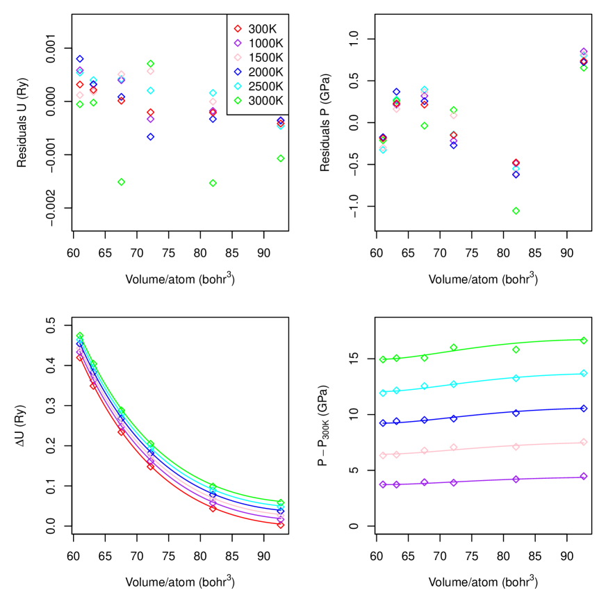
Figure 2: The residuals of the fit to Eq. (1) for the EoS of fcc iridium are shown in a) and b). $\Delta U=U-U_{min}$, where $U_{min}$ is the minimum in the dataset underlined in Table 1. The fitted curves are compared against the dataset in c) and d). $\Delta U$ and thermal pressure $P-P_{\mathrm{300K}}$ from the fit align well against the dataset.

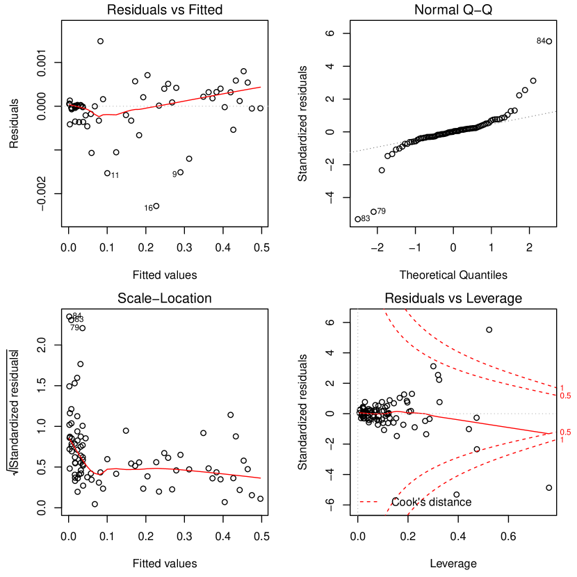
Figure 12: The fit summary plot from the lm function in R.

The residual is the deviation between the target function and the sample mean. From Fig. 2, we observe that the residuals are randomly distributed across the volume range. The absolute value of residuals for $U$ and $P$ are less than 0.002 Ry and 1.0 GPa (except for data point at 3000 K). For the internal energy, a global minimum $U_{min}$ is subtracted from the dataset. On the scale of half Ry, the internal energy is well represented. As for the pressure, we computed the pressure differences with respect to the $T=300$ K reference and the fitted curves aligned with the dataset. Only the $T=3000$ K fit is slightly off. The resultant fitting coefficients in atomic unit for both the Debye model and the classical model are tabulated (see Table 2). The statistical summary from lm function is included in the Appendix A (see Fig. 12).

Table 2: Coefficient matrix $A$ in atomic units for the choice of $F_{0}$, the Debye model and the classical model. The root mean squared errors (RMS) in the fitting for the pressure $P$ (in GPa) and the internal energy $U$ (in mRy) are listed.

	$A_{ij}$	$P$ RMS (GPa)	$U$ RMS (mRy)
Debye model	1.904 -62.84 88.81 8175 0 0.008698 -0.1175 0.5574 $6.681\times 10^{-09}$ $-3.752\times 10^{-07}$ $6.321\times 10^{-06}$ $-3.439\times 10^{-05}$	0.5380	0.706
Classical model	1.902 -62.83 88.68 8176 0 0.008676 -0.1171 0.5549 $6.567\times 10^{-09}$ $-3.667\times 10^{-07}$ $6.166\times 10^{-06}$ $-3.347\times 10^{-05}$	0.5378	0.661

III.1 $P-V-T$ EoS

The equilibrium atomic volume ($P=0$ GPa) at 300 K is 14.559 ų, 2.9% larger than the experimental value 14.145 ų. The overestimation of the lattice constants is expected for the PBE exchange-correlation functional. Experimental $P-V$ curves of 300 K isotherm are readily compared with our theoretical predictions. Pressures measured by Akella et al. [5] are underestimated for compression (see Fig. 3), $\Delta V/V_{0}$ larger than 0.05 with $\Delta V=V_{0}-V$. Overall the theoretical 300 K isotherm agrees well with the experiments within the uncertainty especially when the compression is smaller than 0.15 ($P<70$ GPa) [6, 30, 10]. In contrast, the 3rd order BM fit done by Monteseguro et al. [10] sits along our 1000 K isotherm for compression $>0.15$, and reflects the inadequecy of BM EoS at high compression. For comparison, we have also included the FPMD and experimental study of Anzellini et al. [14]. Their $P-V-T$ curves (both theory and experiments) below 80 GPa are obtained using the EoSFit7 package with ingredients such as the third-order BM EoS for the isothermal part. Their FPMD used the local density approximations and smaller energy cutoff (300 eV). Isotherm of 0 K compared well against our 300 K curve at low compression but not at high compression (compression $>$ 0.90). Similar for the isotherms of 1000 K and 3000 K. The shock-wave experiment by Al’tshuler et al. [31, 32, 33] exhibits quite distinct behavior in the $P-V$ curve. Around compression of 0.1, the temperature is pinned slightly above the isotherm of 1000 K and at compression of 0.22 the temperature is close to the 3000 K isotherm. The high compression pressure ($\approx 600$ GPa) of Al’tshuler et al. was mistakenly reported in Ref. [10]. The recent shockwave experimental work by Khishchenko [34] is also compared. We observe the room temperature isotherm of recent work by Khishchenko et al. align almost perfectly with our EoS data. The data by Monteseguro et al. runs along our 1000 K isotherm for compression over 0.1. It is well-known that dynamic compression experiment lead to a temperature rise. Contrary to the claim that the temperature effect is negligible by Monteseguro et al., [10] we believe the temperatures increase (not measured) along the shock compression $P-V$ curve is significant from our predicted EoS.

Figure 3: Theoretical and experimental EoS’s of fcc iridium are compared. The DAC experimental data for Yusenko [30] Monteseguro[10], Cerenius[6], and Akella[5] were compared at 300 K, where the BM EoS’s were available. Experimental and theoretical data from Anzellini [14] are included (pink, green, and yellow lines). The shockwave data (red cross) of Al’tshuler were taken from Ref. [10]. Room temperature isotherm of Khishchenko shock experiments [34] agrees very well against our FPMD results.

Figure 4: The thermal pressure of fcc iridium is roughly linear in $T$.

Thermal pressure measures the pressure change upon temperature increase at constant volume, $P_{th}(V,T)=P(V,T)-P(V,T_{0})$. The thermal pressure is quite linear in $T$ given that $\alpha K_{T}$ ($\alpha$ and $K_{T}$ are the thermal expansivity and the bulk modulus) is constant in the classical regime (above the Debye temperature), expressed as

$$P_{th}(V,T)=\int_{T_{0}}^{T}\!\!dT\left(\frac{\partial P}{\partial T}\right)_{V}=\int_{T_{0}}^{T}\!\!dT\,\alpha K_{T}\,.$$ (3)

An oversimplified linear equation (see Fig.4) could be given to the thermal pressure $P_{th}(T)=\lambda T$, with $\lambda=0.0056$ GPa/K for the equilibrium volume. One could also see the volume dependence is weak from the bottom right panel of Fig. 2.

The equilibrium bulk modulus $B_{0}$ (or inverse compressibility at room temperature and zero pressure) is an important parameter in the EoS formula, such as the Vinet EoS [35, 36]. The fitted bulk modulus is compared against earlier studies (see Table. 3). We note that Cerenius and Dubrovinsky [6] obtained similar bulk modulus, $354$ GPa versus $306$ GPa, by fitting the second order BM EoS with constraint $B_{0}^{\prime}=4$, or third-order BM EoS without constraint both using experimental equilibrium volume. Park et al. obtained the bulk modulus of 399 GPa and 344 GPa for the LDA and GGA functional in DFT, respectively [37]. We note that $B_{0}$ from our fit is close to the accepted value of about 365 GPa and evidently smaller than Cynn’s value 383 GPa [7]. The parameter $B_{0}^{\prime}$ from our model is $5.3$.

Table 3: Experimental equilibrium volume $V_{0}$ (ų per atom), bulk modulus $B_{0}$ (GPa), and $B_{0}^{\prime}$ at room temperature are compared against reported theoretical results. Data and method are briefly summarized, and the original references are given.

Method description	$V_{0}$	$B_{0}$	$B_{0}^{\prime}$	References
	(Å3/at)	(GPa)
Exp. data fitted to 3rd-order BM EoS	14.120	339	5.3	Monteseguro et al. [10]
Exp. data fitted to 3rd-order BM EoS	14.145	383	3.1	Cynn et al. [7]
Exp. data fitted to				Cerenius and Dubrovinsky[6]
2nd-order BM EoS, with $B_{0}^{\prime}=4$	14.173 (exp. value)	354	4.0
3rd-order BM EoS, without constraint	14.173 (exp. value)	306	6.8
DFT data fitted to BM EoS				Park et al. [37], Table 1 and 2
PAW LDA	13.925	399
PAW GGA	14.524	344
FPMD data fitted to 3rd-order BM EoS	14.150	366	5.0	Burakovsky et al. [9]
FPMD data fitted to our EoS	14.559	361	5.3	This work

III.2 Shock compression

High pressure high temperature conditions are generated by laser heating [38] or resistive heating [39] in a DAC or by laser or gas gun [40] driven shock compression. Strong shocks obey the Rankine-Hugoniot,

$$U-U_{0}+\frac{1}{2}(P+P_{0})(V-V_{0})=0\,.$$ (4)

Since the analytical expression for $U,P$ as a function of $V,T$ is known, for each volume $V$, we solve Eq. (4) by searching its root $T$ given the experimental value $V_{0},T_{0}$.

Figure 5: The principle Hugoniot curve from our theoretical EoS (solid black) of fcc Ir is compared against the shockwave experimental data (symbols). Round green is for the STAR Hugoniot [41], square blue for the LANL Hugoniot [42], and diamond orange for Al’tshuler [31, 32], respectively. Computed temperature from the Eq. (4) is shown in red. The dashed extension is beyond the simulation domain.

We compared our predicted principle Hugoniot with available shock experimental data from several facilities [43, 41] (Fig. 5). Our theoretical principle Hugoniot agrees well with that from earlier data of Al’tshuler and LANL March, as well as more recent data of STAR Hugoniot, for $P<200$ GPa. Above 200 GPa, our predicted pressure is higher than that of LANL and STAR but lower than Al’tshuler’s. Our theoretical Hugoniot below 3000 K (shock temperature) are fairly reliable which correspond to pressure less than 200 GPa. The shock temperature, calculated as the solution to Eq. (4), is shown.

III.3 Equation of state parameters

Thermal EoS parameters such as thermal expansivity $\alpha$, isothermal compressibility $\beta_{T}$, Grüneisen parameter $\gamma$, and the heat capacity $C_{V}$ and $C_{P}$ are obtained by differentiation and algebraic manipulation of Eq. (1). We now discuss some of these parameters.

Figure 6: Parameter $\alpha K_{T}$ as a function of temperature for various pressures.

As expected from the thermal pressure, $\alpha K_{T}$ is weakly dependent on the volume and temperature (see Fig. 6). The Grüneisen parameter

$$\gamma=V\left(\frac{\partial P}{\partial U}\right)_{V}=V\frac{\alpha K_{T}}{C_{V}}$$ (5)

is another important parameter. It is used in the Mie-Grüneisen EoS, where $\gamma$ is assumed independent of temperature. The span of $\gamma$ as a function of temperature reduces when the pressure increases (see Fig. 7). For high compressions, it is indeed fairly temperature independent.

Figure 7: Grüneisen parameter $\gamma$ as a function of temperature for various pressures.

Figure 8: The volumetric thermal expansivity $\alpha$ of fcc iridium as a function of pressure at various temperatures. Halvorson and Wimber measured the linear thermal expansion as $\alpha_{t}=a_{0}+a_{1}t+a_{2}t^{2}+a_{3}t^{3}$ with $a_{0}=6.167\times 10^{-6},a_{1}=3.038\times 10^{-9},a_{2}=-0.8448\times 10^{-12},a_{3}=0.5852\times 10^{-15}$, for $t$ expressed in ^∘C [44] at ambient pressure (see inset solid line), where one can show $\alpha=3(L_{0}/L_{t})\alpha_{t}$ for isotropic materials with reference length $L_{0}$.

The volumetric thermal expansivity $\alpha=-1/V(\partial V/\partial T)_{P}$ for isotropic materials is three times the linear thermal expansivity coefficient $\alpha_{L}$, $\alpha=3\alpha_{L}$. $\alpha$ in Fig. 8 is essentially temperature independent but rather volume sensitive. Our theoretical prediction is below the reported experimental value [44], but it is noted that around room temperature, our theory prediction gives the right thermal expansion coefficient. The expansivity has downsized by a factor of 4 when the pressure goes to 300 GPa.

Figure 9: Constant pressure heat capacity $C_{P}$ as a function of temperature (top panel) and pressure (bottom panel). Experimental value at ambient condition is 25.10 $\mathrm{J}\text{\,}{\mathrm{K}}^{-1}\text{\,}{\mathrm{mol}}^{-1}$[45]. The classical model (blue dash-dotted) for 0 GPa starts to deviate for $T$ below 500 K, and approaches the classical limit as $T\to 0$ K. Inset shows the constant volume heat capacity $C_{V}$. Heat capacity largely reduces when pressure goes up.

The heat capacity at high pressures are almost linear above 500 K, see Fig. 9. The higher the temperature, the slope of $C_{P}$ is smaller. At  0 GPa, the predicted value 25.68 $\mathrm{J}\text{\,}{\mathrm{K}}^{-1}\text{\,}{\mathrm{mol}}^{-1}$is fairly accurate and only 2.3% larger than the experimental heat capacity 25.10 $\mathrm{J}\text{\,}{\mathrm{K}}^{-1}\text{\,}{\mathrm{mol}}^{-1}$[45], given that we used the formula, $C_{P}=C_{V}(1+T\alpha\gamma)$ (see Appendix A) with errors in $C_{V},\alpha,$ and $\gamma$.

The RMSD is a critical quantity for the analysis of the phonon vibrations. Moseley et al. [46] presented temperature-dependent inelastic neutron scattering (INS) experiments as well as quasi-harmonic density functional theory calculations to study the thermodynamic properties of Ir. Our FPMD RMSD at 300 K agrees particularly well with their experimental findings. Their reported $\langle u^{2}\rangle$ at higher temperatures (T=673 K and 823 K, see Table I of Ref. [46]) however, are higher than our FPMD predictions. This is reasonable since our NVT ensembles at these temperatures lead to higher pressure and confined vibrations. It is worth to note that their phonon density of states (PDOS) integrates to 1, and is not fitted well at higher energies. Further investigation of PDOS with a FPMD simulation to compare against the experiments may give insight to the anharmonic effects. Debye temperatures of isochores using Eq. (2) exhibit weak temperature dependence(see Fig. 11).

Figure 10: RMSD as a function of temperature. Experimental data was obtained by Moseley et al. [46] for constant pressure.

Figure 11: Debye temperature ${\Theta_{\mathrm{D}}}$ as a function of temperature. Zero point motion is not included to obtain the Debye temperature. In the high temperature, classical region, our RMSD are classical from classical FPMD (Fig. 10) but when an effective classical Debye temperature is derived to model the RMSD, there is a large change with decreasing temperature into to quantum regime in the Debye model. A 4th order polynomial fit is done only for higher temperature due to the classical treatment to the ions.

IV Conclusions

We have performed a series of FPMD simulations for the fcc Ir at conditions up to 3000 K and 540 GPa. By using a simplified model for the free-energy as a function of temperature and volume and the statistical average quantities internal energy and pressure $(U,P)$, the thermal EoS is obtained by globally fitting to the model. We have compared previous experimental EoS’s and provided the thermal EoS up to 3000 K, and 540 GPa. The $P-V-T$ curve is reasonably agreeing with the fitted BM EoS at low compression but differs at high compression. Our first-principles EoS accords with the most recent shockwave experiment work by Khishchenko We find that $\alpha K_{T}$ and the thermal pressure is quite constant from its dependence in temperature and which turns out to be true for a wide range of materials. We have shown some representative derived thermal parameters against available experiments and found agreements and discrepancies. Further work might resolve these discrepancies.

V Acknowledgments

The work was done under the auspices of the US National Science Foundation CSEDI grant EAR-1901813 to R.E.C. and the National Natural Science Foundation of China (Grant No. 12104230) to K.L.; R.E.C. is supported by the Carnegie Institution for Science and gratefully acknowledges the Gauss Centre for Supercomputing e.V. for funding this project by providing computing time on the GCS Supercomputer Supermuc-NG at Leibniz Supercomputing Centre. All the FPMD calculations were performed on Supermuc-NG.

Appendix A Thermodynamic relations

Once the Helmholtz free energy $F=F(V,T)$ is known as a function of volume ($V$) and temperature ($T$), the following thermodynamical quantities can be obtained from it [47]:

$$P = -\left(\frac{\partial F}{\partial V}\right)_{T}\,,$$ (6)

$$S = -\left(\frac{\partial F}{\partial T}\right)_{V}\,,$$ (7)

$$K_{T} = \beta_{T}^{-1}=-V\left(\frac{\partial P}{\partial V}\right)_{T}=V\left(\frac{\partial^{2}F}{\partial V^{2}}\right)_{T}\,,$$ (8)

$$C_{V} = T\left(\frac{\partial S}{\partial T}\right)_{V}=-T\left(\frac{\partial^{2}F}{\partial T^{2}}\right)_{V}\,,$$ (9)

$$\alpha K_{T} = -\left(\frac{\partial^{2}F}{\partial T\partial V}\right)\,,$$ (10)

$$\gamma = V\left(\frac{\partial P}{\partial U}\right)_{V}=V\frac{\alpha K_{T}}{C_{V}}\,,$$ (11)

$$\frac{C_{P}}{C_{V}} = \frac{K_{S}}{K_{T}}=1+T\alpha\gamma\,,$$ (12)

$$U = F+TS\,,$$ (13)

where pressure, entropy, isothermal compressibility (its inverse is the bulk modulus $K_{T}$), constant volume molar heat capacity, volumetric expansion coefficient, Grüneisen parameter, internal energy are denoted by $P,S,\beta_{T},C_{V},\alpha,\gamma,U$. $C_{P}$ is the constant pressure molar heat capacity. The parameter $B_{0}^{\prime}$ (or $K_{0}^{\prime}=\left.\frac{\partial K}{\partial P}\right|_{P=0}$) can thus be computed using above relations:

$$K^{\prime} = \frac{\partial K}{\partial P}$$ (14)

$$= \left(\frac{\partial K}{\partial T}\right)_{V}\left(\frac{\partial T}{\partial P}\right)_{V}+\left(\frac{\partial K}{\partial V}\right)_{T}\left(\frac{\partial V}{\partial P}\right)_{T}$$

$$= \left(\frac{\partial K}{\partial T}\right)_{V}\frac{1}{\left(\frac{\partial P}{\partial T}\right)_{V}}+\left(\frac{\partial K}{\partial V}\right)_{T}\frac{1}{\left(\frac{\partial P}{\partial V}\right)_{T}}$$

$$= \left(\frac{\partial K}{\partial T}\right)_{V}\frac{1}{\left(\frac{\partial P}{\partial T}\right)_{V}}-\left(\frac{\partial K}{\partial V}\right)_{T}\frac{V}{K_{T}}\,.$$

Appendix B Debye Model

The Helmholtz free energy $F$ of a vibrating lattice at volume $V$ and temperature $T$, can be approximated as

$$F(V,T)=E(V)+F_{\mathrm{vib}}(V,T)+F_{el}(V,T)\,,$$ (15)

where $F_{\mathrm{vib}}$ is the vibrating energy of the lattice and $F_{el}$ is the thermal electronic free energy which is typically negligible. Moruzzi et al. [28] proposed an empirical Debye model with

$$F_{\mathrm{vib}}=k_{B}T\left[-D_{3}(x)+3\ln(1-e^{-x})\right]+\frac{9}{8}k_{B}{\Theta_{\mathrm{D}}}\,,$$ (16)

with Debye temperature ${\Theta_{\mathrm{D}}}$ and dimensionless parameter $x=\frac{{\Theta_{\mathrm{D}}}}{T}$. The last term is the zero-point energy. $D_{3}(x)$ is the third order Debye function. The $n$th order Debye function is defined as

$$D_{n}(x)=\int_{0}^{x}\frac{t^{n}}{e^{t}-1}dt,x\geq 0\,,$$ (17)

where $n$, a non-negative integer, is the order of the Debye function. The vibrational entropy is

$$S_{\mathrm{vib}}=4k_{B}D(x)-3k_{B}\ln(1-e^{-x})\,.$$ (18)

Neglecting the zero-point motion, the vibrational internal energy $U_{\mathrm{vib}}$ thus can be obtained

$$U_{\mathrm{vib}}=F_{\mathrm{vib}}+TS_{\mathrm{vib}}=3k_{B}TD(x)\,.$$ (19)

References

- Arblaster [2010] J. W. Arblaster, Platinum Metals Review 54, 93 (2010).
- Bridgman [1937] P. W. Bridgman, Proceedings of the American Academy of Arts and Sciences 71, 387 (1937).
- Bridgman [1952] P. W. Bridgman, Proceedings of the American Academy of Arts and Sciences 81, 165 (1952).
- Schock and Johnson [1971] B. Schock and Q. Johnson, Fiz . Metal. Metalloved. 31, 1101 (1971).
- Akella [1982] J. Akella, Journal of Physics and Chemistry of Solids 43, 941 (1982).
- Cerenius and Dubrovinsky [2000] Y. Cerenius and L. Dubrovinsky, Journal of Alloys and Compounds 306, 26 (2000).
- Cynn et al. [2002] H. Cynn, J. E. Klepeis, C.-S. Yoo, and D. A. Young, Phys. Rev. Lett. 88, 135701 (2002).
- Baroni et al. [2001] S. Baroni, S. de Gironcoli, A. Dal Corso, and P. Giannozzi, Rev. Mod. Phys. 73, 515 (2001).
- Burakovsky et al. [2016] L. Burakovsky, N. Burakovsky, M. J. Cawkwell, D. L. Preston, D. Errandonea, and S. I. Simak, Phys. Rev. B 94, 094112 (2016).
- Monteseguro et al. [2019] V. Monteseguro, J. Sans, V. Cuartero, F. Cova, I. A. Abrikosov, W. Olovsson, C. Popescu, S. Pascarelli, G. Garbarino, H. J. M. Jönsson, et al., Scientific reports 9, 1 (2019).
- Fang et al. [2010] H. Fang, B. Liu, M. Gu, X. Liu, S. Huang, C. Ni, Z. Li, and R. Wang, Physica B: Condensed Matter 405, 732 (2010).
- Kaptay [2015] G. Kaptay, J. Mater. Sci. 50, 678 (2015).
- Birch [1947] F. Birch, Phys. Rev. 71, 809 (1947).
- Anzellini et al. [2021] S. Anzellini, L. Burakovsky, R. Turnbull, E. Bandiello, and D. Errandonea, Crystals 11 (2021), 10.3390/cryst11040452.
- Kohn and Sham [1965] W. Kohn and L. J. Sham, Phys. Rev. 140, A1133 (1965).
- Mermin [1965] N. D. Mermin, Phys. Rev. 137, A1441 (1965).
- Karasiev et al. [2014] V. V. Karasiev, T. Sjostrom, J. Dufty, and S. B. Trickey, Phys. Rev. Lett. 112, 076403 (2014).
- Karasiev et al. [2016] V. V. Karasiev, L. Calderín, and S. B. Trickey, Phys. Rev. E 93, 063207 (2016).
- Karasiev et al. [2018] V. V. Karasiev, J. W. Dufty, and S. B. Trickey, Phys. Rev. Lett. 120, 076401 (2018).
- Giannozzi et al. [2009] P. Giannozzi, S. Baroni, N. Bonini, M. Calandra, R. Car, C. Cavazzoni, D. Ceresoli, G. L. Chiarotti, M. Cococcioni, I. Dabo, A. D. Corso, S. de Gironcoli, S. Fabris, G. Fratesi, R. Gebauer, U. Gerstmann, C. Gougoussis, A. Kokalj, M. Lazzeri, L. Martin-Samos, N. Marzari, F. Mauri, R. Mazzarello, S. Paolini, A. Pasquarello, L. Paulatto, C. Sbraccia, S. Scandolo, G. Sclauzero, A. P. Seitsonen, A. Smogunov, P. Umari, and R. M. Wentzcovitch, Journal of Physics: Condensed Matter 21, 395502 (2009).
- Garrity et al. [2014] K. F. Garrity, J. W. Bennett, K. M. Rabe, and D. Vanderbilt, Computational Materials Science 81, 446 (2014).
- Perdew et al. [1996] J. P. Perdew, K. Burke, and M. Ernzerhof, Physical Review Letters 77, 3865 (1996).
- Perdew et al. [1997] J. P. Perdew, K. Burke, and M. Ernzerhof, Phys. Rev. Lett. 78, 1396 (1997).
- [24] http://elk.sourceforge.net/, .
- Bussi et al. [2007] G. Bussi, D. Donadio, and M. Parrinello, The Journal of Chemical Physics 126, 014101 (2007).
- Cohen and Gülseren [2001] R. E. Cohen and O. Gülseren, Phys. Rev. B 63, 224101 (2001).
- De Koker and Stixrude [2009] N. De Koker and L. Stixrude, Geophysical Journal International 178, 162 (2009), https://academic.oup.com/gji/article-pdf/178/1/162/5992596/178-1-162.pdf .
- Moruzzi et al. [1988] V. L. Moruzzi, J. F. Janak, and K. Schwarz, Phys. Rev. B 37, 790 (1988).
- Wallace [1965] D. C. Wallace, Phys. Rev. 139, A877 (1965).
- Yusenko et al. [2019] K. V. Yusenko, S. Khandarkhaeva, T. Fedotenko, A. Pakhomova, S. A. Gromilov, L. Dubrovinsky, and N. Dubrovinskaia, Journal of Alloys and Compounds 788, 212 (2019).
- Al'tshuler and Bakanova [1969] L. V. Al'tshuler and A. A. Bakanova, Soviet Physics Uspekhi 11, 678 (1969).
- Al’Tshuler et al. [1981] L. Al’Tshuler, A. Bakanova, I. Dudoladov, E. Dynin, R. Trunin, and B. Chekin, Journal of Applied Mechanics and Technical Physics 22, 145 (1981).
- Nemoshkalenko et al. [1988] V. Nemoshkalenko, V. Y. Mil’Man, A. Zhalko-Titarenko, V. Antonov, and Y. L. Shitikov, Soviet Journal of Experimental and Theoretical Physics Letters 47, 295 (1988).
- Khishchenko [2022] K. V. Khishchenko, Journal of Physics: Conference Series 2154, 012009 (2022).
- Vinet et al. [1986] P. Vinet, J. Ferrante, J. R. Smith, and J. H. Rose, Journal of Physics C: Solid State Physics 19, L467 (1986).
- Vinet et al. [1987] P. Vinet, J. R. Smith, J. Ferrante, and J. H. Rose, Phys. Rev. B 35, 1945 (1987).
- Park et al. [2015] J. Park, B. D. Yu, and S. Hong, Current Applied Physics 15, 885 (2015).
- Meng et al. [2006] Y. Meng, G. Shen, and H. K. Mao, J. Phys.: Condens. Matter 18, S1097 (2006).
- Boehler [1993] R. Boehler, Nature 363, 534 (1993).
- Mitchell and Nellis [1981] A. C. Mitchell and W. J. Nellis, Review of Scientific Instruments 52, 347 (1981), https://doi.org/10.1063/1.1136602 .
- Seagle et al. [2019] C. Seagle, W. Reinhart, S. Alexander, J. Brown, and J.-P. Davis, “Shock compression of iridium,” 21st Biennial Conference of the APS Topical Group on Shock Compression of Condensed Matter (2019).
- Marsh [1980] S. P. Marsh, LASL shock Hugoniot data (University of California press, 1980).
- Fortov et al. [2013] V. Fortov, L. Altshuler, R. Trunin, and A. Funtikov, High-Pressure Shock Compression of Solids VII: Shock Waves and Extreme States of Matter, Shock Wave and High Pressure Phenomena (Springer New York, 2013).
- Halvorson and Wimber [1972] J. J. Halvorson and R. T. Wimber, Journal of Applied Physics 43, 2519 (1972), https://doi.org/10.1063/1.1661553 .
- Lide [2004] D. R. Lide, CRC handbook of chemistry and physics, Vol. 85 (CRC Press, 2004).
- Moseley et al. [2020] D. H. Moseley, S. J. Thébaud, L. R. Lindsay, Y. Cheng, D. L. Abernathy, M. E. Manley, and R. P. Hermann, Phys. Rev. Materials 4, 113608 (2020).
- Callen [1998] H. B. Callen, Thermodynamics and an Introduction to Thermostatistics (American Association of Physics Teachers, 1998).