Revisiting Pure State Transformations with Zero Communication

Abstract

It is known that general convertibility of bipartite entangled states is not possible to arbitrary error without some classical communication. While some trade-offs between communication cost and conversion error have been proven, these bounds can be very loose. In particular, there are many cases in which tolerable error might be achievable using zero-communication protocols. In this work we address these cases by deriving the optimal fidelity of pure state conversions under local unitaries as well as local operations and shared randomness (LOSR). We also use these results to explore catalytic conversions between pure states using zero communication.

I Introduction

The theory of quantum mechanics through the lens of information and vice versa [1, 2, 3] has afforded the physicist and the information scientist alike with a new way to view the objects and long-term goals of their study. No better example of this can be found than quantum resource theories. Quantum resource theories specify the relevant physical property in such a manner as to better tease apart the complexities of quantum mechanics while also establishing what tasks may be achieved with said resource [4]. Perhaps the earliest example of such a resource theory is the resource theory of entanglement. Entanglement may be viewed as a form of correlation that does not exist in the classical world [5]. Roughly speaking, the resource theory of entanglement asks (1) what tasks may be performed better using entangled states and (2) how entangled states may be converted from one to another under some class of free operations.

The most standard view of the resource theory of entanglement considers the set of free operations to be local operations and classical communication (LOCC) which captures the ‘distant lab’ paradigm where two (or more) parties share an entangled state in spatially separated labs and they can only perform operations on their respective portions and exchange classical information (See Fig. 1). Not only is this the most standard set of free operations, but in some respect it seems minimal. Indeed, Hayden and Winter showed that to convert one (pure) entangled state to another to sufficiently small precision requires a certain amount of communication between labs, regardless of how many auxiliary EPR pairs they share [6] (see also [7]). This is distinct not only from the classical setting [8], but also from quantum states that are not entangled [9, 10]. However, the results of Hayden and Winter, while fundamental, do not give us a complete picture of the tradeoff between communication and achievable tolerated error in pure state conversions. Indeed, it is easy to find examples of state conversions which, according to the best known lower bounds, still may be possible to perform with a tolerated error of $1\%$ using no communication (see Example 1 of Section III). This show that a relatively large gap in our understanding of zero-communication entanglement transformations still persists, and one we aim to address in this work.

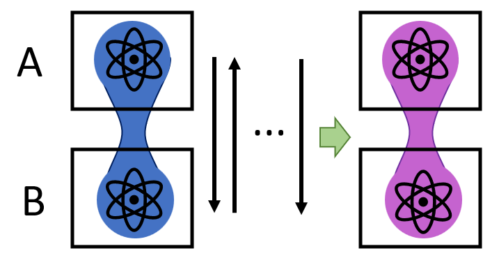
(a)

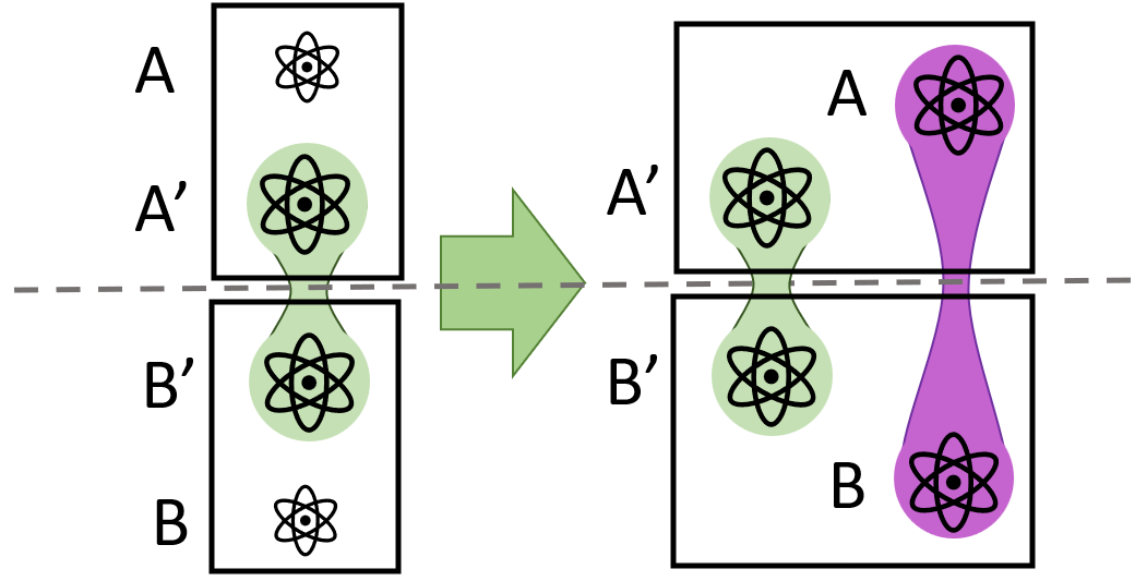
(b)

Figure 1: Conversion of pure states in distant labs. (a) The LOCC model where communication is exchanged. (b) The embezzling of quantum states where an auxiliary entangled state is used. This may be seen as a special case of catalytic conversion.

Moreover, the tools we develop to address this problem will also allow us to study pure state transformations using shared auxiliary entanglement. The operational paradigm in which parties are allowed to use arbitrary pre-shared entanglement but no communication is known as local operations and shared entanglement (LOSE) [11]. By itself, the problem of pure state convertibility $\ket{\psi}_{AB}\to\ket{\phi}_{AB}$ under LOSE is trivial since Alice and Bob could always just demand $\ket{\phi}$ as their pre-shared entanglement and then throw away $\ket{\psi}$ when it is given. However, if one demands that the pre-shared entanglement is also returned in addition to the target state $\ket{\phi}$, then the problem becomes quite interesting, i.e. $\ket{\psi}_{AB}\otimes\ket{\omega}_{A^{\prime}B^{\prime}}\to\ket{\phi}_{AB}\otimes\ket{\omega}_{A^{\prime}B^{\prime}}$ for auxiliary pre-shared entanglement $\ket{\omega}_{A^{\prime}B^{\prime}}$. Transformations of this form are known as catalytic transformations with $\ket{\omega}_{A^{\prime}B}$ being the catalyst. Remarkably, van Dam and Hayden have shown that there exists a family of entangled catalysts, known as universal embezzling states [12], such that for any tolerated non-zero error one can always prepare a pure state using a member of this family and zero communication. More amazingly, they showed that as the error tends to zero, it is roughly optimal since it scales nearly the same as if you add LOCC and allow the catalyst to be state dependent. This near optimality along with Hayden and Winter’s result has, understandably, largely ceased the study of entanglement transformations with zero communication, because when one needs entanglement transformations without communication, one uses embezzlement [13, 14]. It is however not clear what is the necessary error for embezzlement to become near optimal, which could be relevant in practical settings. Indeed, for any tolerated error, it is easy to find sufficient conditions on pure states to be converted with no catalyst at all (Example 2 of Section III). This is an indication that we also do not understand embezzling and catalytic convertibility sufficiently well.

I.1 Summary of Results

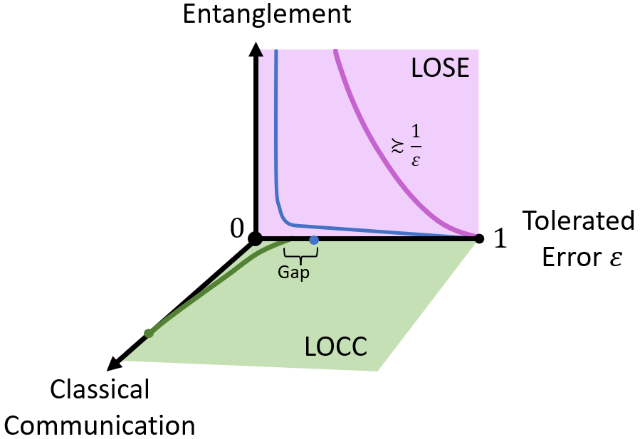
Figure 2: Comparison of [12] (dark pink),[17] (dark green), and this work’s results (blue). [17] finds lower bounds on the classical communication necessary to convert one state to another, but in the zero communication setting these are too loose. We find methods for solving this exactly (Section IV), which establishes that communication is necessary for larger tolerated errors. [12] establishes a method for pure state transformations with zero communication with massive amounts of entanglement, but it scales inversely with the error, which we find can be too strong for a relevant error range, even if ultimately it is optimal (Section VI).

The primary aim of this work is to provide tighter lower bounds on the error in pure state entanglement convertibility with zero communication. A high level comparison of our results to the aforementioned work on this topic are presented in Fig. 2. This depicts a ‘one-shot resource tradeoff’ region that must contain the ‘true’ one-shot resource tradeoff surface for a given pure state conversion. Hayden and Winter’s result provides a lower bound on the achievability independent of the amount of shared maximally entangled states, but their result can be too loose when considering zero communication. van Dam and Hayden’s result provides an outer bound on the achievability surface on the face pertaining to LOSE, but their result in fact can be too loose when the error is not sufficiently small. In this work, our results allow one to exactly solve the minimal error in the zero communication setting and also provide significantly tighter bounds than quantum embezzling for a relevant region on the LOSE face (See Fig. 2).

To formally establish our results, we reduce the class of questions regarding optimal pure state conversion to optimization problems that only concern probability distributions. This is because of a bijection between the equivalence classes of pure states under local unitaries— which are defined solely by their Schmidt coefficients— and the probability simplex. We do this by showing the optimal fidelity of pure state transformations with local unitaries is efficiently computable. Of course, in general one would not expect local unitaries to be the optimal strategy and we build on this result to present a non-convex optimization program over an optimization variable with bounded dimension. An immediate corollary of this result is the impossibility of pure state conversions with zero communication for negligible error. We also present efficient computable upper bounds on the achievable error using a semidefinite programming (SDP) relaxation. We also show that in the case where either the seed (i.e. initial) or target state is a two-qubit state, the local unitary strategy is optimal. However, we can show for larger dimensions this is not the case.

Having established general properties in the single copy case, we move to the multiple copy case, i.e. where the seed and/or target state is of independent and identically distributed (i.i.d.) form. This is standard in determining the rate of converting one state to another. In particular, we consider dilution and distillation where the seed state or target state respectively is many copies of a maximally entangled state and show these are convex optimization programs and may be seen as involving the Ky-Fan norms when extended to the regime where they are not a norm. Lastly, in a sense extending our earlier two-qubit results, we establish that if the target state is an $n-$fold copy of a two-qubit entangled state and the seed state’s Schmidt rank is less than the target state, then local unitaries are the optimal strategy.

Finally, given these results, we turn our attention to quantum embezzlement. We begin by noting that the correspondence between Schmidt coefficients and probability distributions means that quantum embezzlement implies a classical equivalent we call randomness embezzlement. We then proceed to use our new tools to consider the problem of catalyzed pure state conversion under local unitaries, in effect a generalization of embezzling, and compare it to embezzling. We show in particular that at least in general the optimality of the embezzling states is only for very small errors. Indeed, we show for reasonable tolerable errors, the embezzling state may have a Schmidt rank of many orders of magnitude larger than a simple catalyst. This may have practical relevance and strongly refines our understanding of pure state transformations under LOSE.

Organization of the Paper

The rest of the paper is organized as follows. In Sections II and III we present the necessary notation and background respectively to understand the rest of the paper. In Section IV, we

• Make explicit the correspondence between pure states under LU and the probability simplex and note this implies the existence of a classical variation of embezzlement (Theorem 2)

• Prove our equation for fidelity of state conversion under local unitaries (Theorem 5) and our optimization for fidelity of state conversion under local operations and shared randomness (Theorem 6)

• Establish computable upper bounds on the fidelity of state conversion under LOSR (Theorem 9).

In Section V we present the results where the target or seed state is of i.i.d. form. In Section VI we discuss catalysts under local unitaries, the general frameworks that includes quantum embezzlement,. In Section VII we discuss why our theory does not generalize beyond bipartite pure states.

II Notation

Our notation largely aligns with standard texts [18, 19]. In this paper we consider finite dimensional quantum systems. Given $n\in\mathbb{N}$, we define $[n]:=\{1,...,n\}$. A finite dimensional Hilbert space will be labeled with a capital roman letter, e.g. $A,B,$ etc. As they are finite dimensional, these Hilbert spaces may be identified by the isomorphism $A\cong\mathbb{C}^{d}$ where $d\in\mathbb{N}$. The space of linear maps from a Hilbert space $A$ into itself, i.e. the space of endomorphisms, is denoted $\mathrm{L}(A)$. The space of quantum states, or density matrices, with respect to a Hilbert space $A$, is the space of positive semidefinite operators with unit trace, i.e.  $\mathrm{D}(A):=\{\rho\in\mathrm{L}(A):\rho\succeq 0\,\&\Tr(\rho)=1\}$ where $\succeq$ is the Löwner order. If a quantum state is a joint state over multiple Hilbert spaces, we will use a subscript to specify this, e.g. $\rho_{AB}\in\mathrm{D}(A\otimes B)$. We say a quantum state $\rho_{A}\in\mathrm{D}(A)$ is pure if $\Tr(\rho^{2}_{A})=1$ which is equivalent to there being a unit vector $\ket{\psi}\in A$ such that $\rho_{A}=\outerproduct{\psi}{\psi}$, where we are using bra-ket notation. For this previous reason, we generally just specify a pure state by $\ket{\psi}_{A}$, or $\psi$ if we are considering its density matrix representation. We denote the space of pure states $\mathcal{S}(A)$, where $\mathcal{S}$ stands for unit sphere.

A state is classical if it is diagonal in a specific choice of basis for $\mathrm{L}(A)$. We call this the computational basis. The space of classical probability distributions over $d$ elements, the probability simplex which we denote $\mathcal{P}(d)$, may be viewed as the set of non-negative $d-$dimensional vectors that sum to one or the set of diagonal density matrices in the computational basis. To distinguish between the two, we write $P$ for the matrix version and $p$ for the vector version. We also define the set of entry-wise decreasing probability distributions over $d$ elements, i.e. elements of the form $p^{\downarrow}(1)\geq p^{\downarrow}(2)\geq...\geq p^{\downarrow}(d)$, by $\mathcal{P}^{\downarrow}(d)$.

A quantum channel $\mathcal{E}\in\mathrm{C}(A,B)$ is a (linear) completely positive, trace preserving map $\mathcal{E}:\mathrm{L}(A)\to\mathrm{L}(B)$. Any quantum channel admits an isometric representation, e.g. given $\mathcal{E}\in\mathrm{C}(A,B)$, there exists a Hilbert space $E$ such that $|E|\leq|A||B|$ and isometry $V:A\to B\otimes E$ such that $\Phi(X)=\Tr_{E}(VXV^{\dagger})$ where $\Tr_{E}$ is the partial trace on the $E$ space and $X^{\dagger}$ is the Hermitian conjugate.

Given the space of linear operators from $A\cong\mathbb{C}^{d}$ to $B\cong\mathbb{C}^{d^{\prime}}$, $\mathrm{L}(A,B)$, the vec mapping $\operatorname{vec}:\mathrm{L}(A\otimes B)\to A\otimes B$ is defined by $\operatorname{vec}(\ket{i}\bra{j})=\ket{j}\otimes\ket{i}$ where $\{\ket{i}\}_{i\in[d]}$ and $\{\ket{j}\}_{j\in[d^{\prime}]}$ are the computational bases for $A$ and $B$ respectively. This choice of vec mapping satisfies the identity

$$(X_{1}^{T}\otimes X_{0})\operatorname{vec}(Y)=\operatorname{vec}(X_{0}YX_{1})\ ,$$ (1)

where $X_{0}\in\mathrm{L}(A_{0},B_{0})$, $X_{1}\in\mathrm{L}(A_{1},B_{1})$, and $Y\in\mathrm{L}(B_{1},B_{0})$. The vec mapping is also an isometry in the sense that for all $X,Y\in\mathrm{L}(A,B)$,

$$\langle X,Y\rangle=\langle\operatorname{vec}(X),\operatorname{vec}(Y)\rangle\ ,$$

where $\langle\cdot,\cdot\rangle$ on the L.H.S. is the inner product on $\mathrm{L}(A,B)$ defined by $\langle X,Y\rangle=\Tr(X^{\dagger}Y)$ and the R.H.S. is the inner product on vectors $A\otimes B$ defined by $\bra{\psi}\ket{\phi}=\sum_{i}\overline{\psi(i)}\phi(i)$ where $\overline{\cdot}$ is the conjugate.

III Background & Motivation

Throughout this section we fix $A\cong\mathbb{C}^{d},B\cong\mathbb{C}^{d^{\prime}}$ for clarity.

Fidelity

The fidelity is a standard measure of similarity between two positive semidefinite operators $R,S\geq 0$.

$$F(R,S)=\left\|\sqrt{R}\sqrt{S}\right\|_{1}^{2}=\Tr\left(\sqrt{\sqrt{S}R\sqrt{S}}\right)^{2}\ ,$$ (2)

where the square root of a positive semidefinite operator is defined in the standard fashion on its spectral decomposition and $\|\cdot\|_{1}$ is the Schatten $1-$norm. It satisfies various properties that will be relevant for this work which we summarize here. All of these may be verified by direct calculation or by referring to standard texts.

Proposition 1 (Summary of Fidelity Properties).

Let $\rho,\sigma\in\mathrm{D}(A)$. The following hold:

1. $0\leq F(\rho,\sigma)\leq 1$ where the upper bound is saturated if and only if $\rho=\sigma$ and the lower bound saturates if and only if their images are orthogonal.

2. The fidelity is isometrically invariant, i.e. given isometry $V:A\to B$,

   $$F(V\rho V^{\dagger},V\sigma V^{\dagger})=F(\rho,\sigma)\ .$$

3. The fidelity satisfies data-processing. That is, for any quantum channel $\mathcal{E}\in\mathrm{C}(A,B)$,

   $$F(\rho,\sigma)\leq F(\mathcal{E}(\rho),\mathcal{E}(\sigma))\ .$$

4. If both states are pure,

   $$F(\outerproduct{\phi}{\phi},\outerproduct{\psi}{\psi})=|\bra{\psi}\ket{\phi}|^{2}\ ,$$

   and if one state is pure

   $$F(\outerproduct{\phi}{\phi},\sigma)=\bra{\phi}\sigma\ket{\phi}\ .$$

5. If both states are classical, $P,Q\in\mathcal{P}(d)$, then the fidelity reduces to the square of the Bhattacharyya coefficient:

   $$\hskip 28.45274ptF(P,Q)=\left(\sum_{i\in[d]}\sqrt{p(i)q(i)}\right)^{2}=BC(p,q)^{2}\ ,$$

   where $p(i)=P(i,i)$ and likewise for $Q$.

6. Given pure states with the same eigenbasis and real amplitudes, $\ket{\psi}=\sum_{x}\sqrt{p(x)}\ket{x}$, $\ket{\phi}=\sum_{x}\sqrt{q(x)}\ket{x}$ , the fidelity reduces to the square of the Bhattacharyya coefficient of the probability distributions defined by the amplitudes:

   $$F(\outerproduct{\phi}{\phi},\outerproduct{\psi}{\psi})=BC(p,q)^{2}\ .$$

We also note that in all of these definitions there is a pesky squaring that effectively we don’t care about. For this reason we could define the square root fidelity:

$$\sqrt{F}(R,S):=\sqrt{F(R,S)}\ .$$

Note the square root fidelity could be viewed as the quantum extension of the Bhattacharyya coefficient.

Norms

In defining the fidelity we used the Schatten $1-$norm. More generally, there are the Schatten $p-$norms which for $X\in\mathrm{L}(A,B)$ may be defined as $\|X\|_{p}:=\|\sigma(X)\|_{p}$ where $\sigma(X)$ is the ordered vector of singular values of $X$, $\sigma_{1}(X)\geq\sigma_{2}(X)\geq...\geq\sigma_{\mathrm{rank}(X)}(X)$ and it is being evaluated under the $L_{p}-$norm where $p\geq 1$. The infinity norm, $\infty-$norm, is $\lim_{p\to\infty}\|X\|_{p}=\|X\|_{\infty}=\max_{i}\sigma_{i}(X)$. The infinity norm was generalized to the Ky Fan $k-$norms $\|X\|_{(k)}:=\sum\sigma_{i}(X)$ for $1\leq k\leq\min\{d,d^{\prime}\}$. The Ky Fan norms have relevance in measuring entanglement [20]. A generalization of the Ky Fan and Schatten norms together is given by the $(k,p)-$norms [21]

$$\|X\|_{(k,p)}:=\left(\sum_{i\in[k]}\sigma_{i}(X)^{p}\right)^{1/p}\ ,$$ (3)

which also have use in measuring entanglement of pure states [22]. Much like is common to do for the Schatten $p-$norms, we can extend the $(k,p)-$norms to $p>0$ with the caveat they won’t be norms as they won’t in general satisfy subadditivity (the triangle inequality) for $p\in[0,1)$.

Entanglement Theory

A bipartite quantum state $\rho_{AB}$ is separable if there exists $n\in\mathbb{N}$, $p\in\mathcal{P}(n)$, $\{\sigma_{A}^{i}\}_{i\in[n]}\subset\mathrm{D}(A)$, and $\{\tau_{B}^{i}\}_{i\in[n]}$ such that

$$\rho_{AB}=\sum_{i\in[n]}p(i)\sigma_{A}^{i}\otimes\tau_{B}^{i}\ .$$

Otherwise the state is entangled. As a pure state $\outerproduct{\psi}{\psi}_{AB}$ is defined by a unit vector, this reduces to a pure state is separable, referred to product in this setting, if and only if there exists $\ket{\phi}_{A},\ket{\varphi}_{B}$ such that $\ket{\psi}=\ket{\phi}_{A}\otimes\ket{\varphi}_{B}$. While this is sufficient for determining if a bipartite pure state is entangled, there is also a notion of ‘how’ entangled a state is in terms of Schmidt rank. Every bipartite pure state $\ket{\psi}_{AB}$ admits a unique (up to re-ordering) decomposition of the form

$$\ket{\psi}_{AB}=\sum_{i\in[k]}\sqrt{p(i)}\ket{u_{i}}_{A}\otimes\ket{v_{i}}_{B}\ ,$$ (4)

where $k=\max\{d,d^{\prime}\}$, $p\in\mathcal{P}(k)$ and $\{\ket{u_{i}}\}_{i\in[k]},\{\ket{v_{i}}\}_{i\in[k]}$ are orthonormal bases of $A$ and $B$ respectively. The $\sqrt{p(i)}>0$ terms are referred to as the Schmidt coefficients. The Schmidt rank of $\ket{\psi}_{AB}$, $\mathrm{SR}(\ket{\psi})=\mathrm{supp}(p)$, i.e. the number of Schmidt coefficients. This may be viewed as a measure of entanglement in the sense that the Schmidt rank of a product state is 1 and the maximally entangled state $\ket{\Phi^{+}}_{\mathbb{C}^{d}\mathbb{C}^{d}}=\frac{1}{\sqrt{d}}\sum_{i}\ket{i}_{\mathbb{C}^{d}}\ket{i}_{\mathbb{C}^{d}}$ has Schmidt rank $d$. We define the set $\mathrm{SR}(d):=\{\ket{\psi}:\mathrm{SR}(\ket{\psi})\leq d\}$, where we note this set is independent of the dimension the state is embedded in.

Lastly we note a particularly nice property of pure states, known as Uhlmann’s theorem.

Lemma 1 (Uhlmann’s Theorem).

Given $\rho,\sigma\in\mathrm{D}(A)$ and $\ket{\psi}\in A\otimes B$ such that $\Tr_{B}(\psi)=\rho$, then

$$F(\rho,\sigma)=\max\{|\bra{\psi}\ket{\phi}|^{2}:\ket{\phi}\in A\otimes B\,,\,\Tr_{B}(\phi)=\sigma\}\ .$$

No-Go Theorems, Embezzling, & Motivation

With the established background, we now present the previous results related to zero communication pure state transformations which we will discuss our results in relation to. The first is a lower bound on the number of qubits or classical bits necessary to convert between pure states [6].

Proposition 2.

([6, Theorem 8]) Consider a state transformation via channel $\mathcal{E}\in\mathrm{C}(A\otimes B,A\otimes B)$ from seed state $\ket{\phi}_{AB}$ to target state $\ket{\psi}_{AB}$ such that $F(\mathcal{E}(\phi),\psi)\geq 1-\varepsilon$. Then, independent of any amount of entanglement assistance, for $\delta=\sqrt[8]{\varepsilon}$, in the implementation of $\mathcal{E}$, $q$ qubits were exchanged where

$$q\geq \frac{1}{2}\left[\Delta_{\delta}(\Tr_{B}(\outerproduct{\phi}{\phi}))-\Delta_{0}(\Tr_{B}(\outerproduct{\psi}{\psi}))\right]$$ (5)

$$\hskip 113.81102pt+\log(1-\delta)\ ,$$

where

$$\exp(\Delta_{\varepsilon}(P))=\min \operatorname{rank}(\widetilde{P})\cdot\lambda_{\max}(\widetilde{P})$$

s.t. $$\Tr(\widetilde{P})\geq 1-\varepsilon$$

$$\,\widetilde{P}=\Pi P\Pi\,$$

$$\,[P,\Pi]=0$$

$$\,\Pi^{2}=\Pi\ .$$

Moreover, the bound given in (5) holds for a necessary amount of classical communication by multiplying the R.H.S. by two.

While the above proposition is very powerful and implies two states with different Schmidt decompositions cannot be perfectly converted with zero communication, it is not sufficient in every scenario. In particular, the following example shows that in certain cases Proposition 2 cannot eliminate any state from being able to be converted to a given target state with relatively high fidelities.

Example 1 (On the necessity of communication).

Up to local unitaries, let the target state be $\ket{\psi}=0.54\ket{00}+0.02\ket{11}+0.44\ket{22}$, the seed state be any state $\ket{\phi}=\sum_{i\in[k]}\sqrt{p(i)}\ket{v_{i}}\ket{u_{i}}$, and assume we are interested in a state transformation $\mathcal{E}$ such that $F(\mathcal{E}(\phi),\psi)=0.99$. Then $\varepsilon=0.01$, so $\delta>0.56$. One may verify $\Delta_{\delta}(P)=\log(|1|\cdot 0.44)<-1.18$, by removing the $0.02$ and $0.54$ eigenvalues of $P$. It may be shown [6] that $\Delta_{0}(\Tr_{B}(\outerproduct{\psi}{\psi}))\geq 0$, and $\log(1-\delta)<0$. It follows that in this setting the R.H.S. of (5) is negative. Therefore, we have no proof from this bound that any transformation for any seed state which achieves this relatively high fidelity of $99\%$ requires any communication.

While the above example shows there are reasonably small tolerated errors $\varepsilon$ where Proposition 2 is not helpful, when the tolerated error is sufficiently small, it will imply the need for communication. This sort of structure for sufficiently small $\varepsilon$ also appears when considering quantum embezzlement [12], which may be seen as a solution to Proposition 2 implying communication is necessary. Quantum embezzlement in effect shows one can make pure state transformations with zero communication to any non-zero error if they have the right sufficiently large entangled catalyst.

Proposition 3.

([12]) Consider the family of catalyst states $\ket{\mu(n)}_{A^{\prime}B^{\prime}}=\frac{1}{\sqrt{H_{n}}}\sum_{j=1}^{n}\frac{1}{\sqrt{j}}\ket{j}_{A^{\prime}}\ket{j}_{B^{\prime}}$ where $H_{n}:=\sum_{i=1}^{n}n^{-1}$ is the Harmonic number. For any $\varepsilon>0$ and target bipartite pure state $\ket{\psi}_{AB}$ with Schmidt rank $m$, for $n>m^{1/\varepsilon}$ there exist unitaries $U_{AA^{\prime}},W_{BB^{\prime}}$ such that

$$F(U_{AA^{\prime}}\otimes W_{BB^{\prime}}(\ket{\mu(n)}_{A^{\prime}B^{\prime}}\ket{0}_{A}\ket{0}_{B}),$$

$$\hskip 85.35826pt\ket{\mu(n)}_{A^{\prime}B^{\prime}}\otimes\ket{\psi}_{AB})\geq 1-\varepsilon\ .$$

Moreover, $U,W$ are in effect permutations on the joint Schmidt bases.

One can see quantum embezzlement implies a way to convert one pure state to another to non-zero error by picking a large enough catalyst and then first ‘embezzling out’ the original state (uncomputing $\ket{\phi}$ to $\ket{0}\ket{0}$ via embezzling) and then ‘embezzling in’ the target state $\ket{\psi}$.

What is perhaps most remarkable about the above approach is that it was shown in the original work that even if we allow LOCC and a state dependent catalyst, the error scales as $\Omega(1/\log(n))$ whereas for the above result the errors scales as $O(1/\log(n))$, so as the error is driven down, embezzling is near optimal. That is, as $\varepsilon\to 0$, this strategy is effectively optimal. However, just as with the discussion pertaining to Proposition 2, it’s clear embezzling isn’t necessary for reasonable error levels in general. In fact, we show in the following example that for any non-zero error there exist states which can be converted without any catalyst.

Example 2 (On the necessity of embezzling).

As noted, as $\varepsilon\to 0$, embezzling is necessary. However, it is not in general clear at what point embezzling becomes necessary. This can be seen as follows. Consider $\varepsilon\in(0,1)$ and two probability distributions $p,q\in\mathcal{P}(m)$ such that the $\mathrm{BC}(p,q)^{2}\geq 1-\varepsilon$. Define the seed state as $\ket{\phi}=\sum_{i\in[m]}\sqrt{p(i)}\ket{i}_{A}\ket{i}_{B}$ and the target state as $\ket{\psi}=\sum_{i\in[m]}\sqrt{q(i)}\ket{i}_{A}\ket{i}_{B}$. Then we have

$$F(\outerproduct{\phi}{\phi},\outerproduct{\psi}{\psi})=BC(p,q)^{2}\geq 1-\varepsilon\ ,$$

where we have used Item 5 of Proposition 1. Therefore, given $\ket{\phi}$, it requires no communication or entanglement to generate $\ket{\psi}$ to error $\varepsilon$. In fact, as we show later (Proposition 4), this will be true for converting the set of states with Schmidt coefficients defined via $p$ to the set of states with Schmidt coefficients defined via $q$ in general.

Given these two examples, we see that while these results give strong characterizations of pure state transformations with zero communication, neither the need for communication by Proposition 2 nor the optimality of Proposition 3 when the error tends to zero give us a full understanding of this setting. It would therefore be of value to better understand this task, and this is what the rest of this work addresses.

IV Single Copy Pure State Conversion with Zero Communication

Our primary goal of this section is to determine the minimal error of conversion between pure states with zero communication, which would resolve the gap presented in Example 1. To do this, we will use the correspondence between the probability simplex and Schmidt coefficients under local unitaries (LU), which we establish in the following subsection. We also note that this implies the existence of a classical equivalent of embezzling, which we call randomness embezzling (Theorem 2). This correspondence motivates the idea that the optimal fidelity of pure state conversion under local unitaries is simply re-ordering the Schmidt coefficients, which we in fact prove (Theorem 5). We then use the local unitary result to establish a bounded but non-linear optimization program that determines the optimal achievable fidelity under conversion via local operations and shared randomness (LOSR), which does not require shared randomness (Theorem 6). We end the section by discussing the relationship between the LU and LOSR strategies and introducing an SDP relaxation for efficiently establishing upper bounds on the achievable fidelity of pure state conversions under LOSR.

IV.1 Correspondence Under Local Unitaries between Schmidt Coefficients and the Probability Simplex

In this subsection we establish the bijection between Schmidt coefficients, which define the equivalence classes of bipartite pure states under local unitaries, and the probability simplex. One reason for this is because the rest of the results of this work might be best seen as verifying that in the zero communication setting this correspondence is all that matters. Indeed, we will see this in the subsequent subsections which show that the minimal fidelity error of pure state transformations under zero communication will always be functions of only the Schmidt coefficients.

Proposition 4.

Up to local unitaries, any pure quantum state is of the form

$$\ket{\psi}_{AB}=\sum_{i\in[k]}\sqrt{p^{\downarrow}(i)}\ket{i}_{A}\otimes\ket{i}_{B}\ ,$$

where $p^{\downarrow}(i)\geq p^{\downarrow}(i+1)$ for all $i\in[k-1]$, $k=\max\{d,d^{\prime}\}$, $p^{\downarrow}\in\mathcal{P}^{\downarrow}(k)$, and $\{\ket{i}\}$ is the computational basis in both cases. In other words, there exist both equivalence classes on pure states under local unitary operations in terms of Schmidt coefficients and ordered Schmidt coefficients.

Proof.

Consider $\ket{\psi}_{AB}=\sum_{j\in[k]}\sqrt{p^{\prime}(j)}\ket{u_{j}}\otimes\ket{v_{j}}$ as decomposed in (4). Now fix the permutation $\pi$ on $[k]$ such that $p^{\prime}(\pi^{-1}(i))\geq p^{\prime}(\pi^{-1}(i+1))$ for all $i\in[k-1]$, i.e. $\pi$ re-labels $p^{\prime}$ so that it is decreasing. Define the unitaries $U_{A}=\sum_{j\in[k]}\ket{\pi(j)}\bra{u_{j}}$, $W_{B}=\sum_{j\in[k]}\ket{\pi(j)}\bra{v_{j}}$, which may be verified to be unitaries by direct calculation. Then $(U_{A}\otimes W_{B})\ket{\psi}_{AB}$ will be of the form given in the proposition statement. Finally, we could make this argument for any pure state without ordering the Schmidt coefficients to get one set of equivalence classes. As such, under local unitaries, we can define equivalence classes of pure states in terms of ordered or non-ordered Schmidt coefficients. This completes the proof. ∎

Definition 1.

The space of (representatives of the equivalence class of) ordered Schmidt coefficient pure states with Schmidt rank bounded by $d$ is given by $\mathrm{SR}^{\downarrow}(d)$. That is, if $\ket{\psi}\in\mathrm{SR}^{\downarrow}(d)$, then $\ket{\psi}=\sum_{i\in[d]}\sqrt{p^{\downarrow}(i)}\ket{u_{i}}\ket{i}\ket{i}$ where $p^{\downarrow}\in\mathcal{P}^{\downarrow}(d)$.

We can use the previous proposition to relate the (ordered) probability simplex over $d$ elements to to the equivalence classes of (ordered) Schmidt decompositions with Schmidt rank bounded by $d$.

Proposition 5.

Consider the functions $\operatorname{vec}(\sqrt{\cdot}):\mathrm{L}(\mathbb{C}^{d})\to\mathbb{C}^{d}\otimes\mathbb{C}^{d}$ and $\operatorname{vec}^{-1}(\cdot^{\odot 2}):\mathbb{C}^{d}\otimes\mathbb{C}^{d}\to\mathrm{L}(\mathbb{C}^{d})$ where $\cdot^{\odot 2}$ is the entry-wise square of a vector. These functions define a bijection between $\mathcal{P}(d)$ (resp. $\mathcal{P}^{\downarrow}(d)$) and the space of equivalence classes of Schmidt decompositions under local unitaries with Schmidt rank bounded by $d$ (resp. the space $\mathrm{SR}^{\downarrow}(d)$.)

Proof.

We prove it via direct calculation for $\mathcal{P}(d)$ and the space of Schmidt decompositions. The proof in the other case works the same. Let $C\cong\mathbb{C}^{d}$. First, consider $p\in\mathcal{P}(d)$ which we write in its density matrix form, e.g. $P=\sum_{i\in[d]}p(i)\outerproduct{i}{i}$. Then

$$\operatorname{vec}(\sqrt{P})= \operatorname{vec}\left(\sum_{i\in[d]}\sqrt{p(i)}\outerproduct{i}{i}\right)$$

$$= \sum_{i\in[d]}\sqrt{p(i)}\ket{i}_{C}\otimes\ket{i}_{C^{\prime}}\ ,$$

which is in the specified equivalence class by applying an isometries that take the computational bases from $C,C^{\prime}$ to $A,B$. In the other direction, take the Schmidt decomposition in the purified basis, $\ket{\psi}_{AB}=\sum_{i\in[d]}\sqrt{q(i)}\ket{i}_{A}\otimes\ket{i}_{B}$. We can convert the $A$ space to $C$ via the channel

$$\mathcal{F}_{A\to C}(\cdot):=V^{\dagger}\cdot V+(\mathbb{1}-V^{\dagger}V)\cdot(\mathbb{1}-V^{\dagger}V)\ ,$$

where $V=\sum_{i\in[d]}\ket{i}_{A}\bra{i}_{C}$ is the isometry that takes the $C$ space to the $A$ space as $|A|\geq|C|$ by assumption. The same type of conversion holds for the $B$ and $C^{\prime}$. Therefore, we have (up to equivalences) $\ket{\psi}_{AB}=\sum_{i\in[d]}\sqrt{q(i)}\ket{i}_{C}\ket{i}_{C^{\prime}}$. Then,

$$\operatorname{vec}^{-1}(\ket{\psi}^{\cdot 2})= \operatorname{vec}^{-1}(\sum_{i\in[d]}q(i)\ket{i}_{C}\ket{i}_{C^{\prime}})$$

$$= \sum_{i\in[d]}q(i)\outerproduct{i}{i}_{C}\ ,$$

where in the last line we used that $C^{\prime}\cong C$ so that $\mathrm{L}(C,C^{\prime})\cong\mathrm{L}(C)$. This completes the proof. ∎

The reason this is useful is it draws equivalence between the equivalence classes of entangled states in terms of Schmidt coefficients and probability distributions under fidelity.

Proposition 6.

Consider $\ket{\phi}=\sum_{i\in[d]}\sqrt{p(i)}\ket{i}_{A}\ket{i}_{B}$, $\ket{\psi}=\sum_{i\in[d]}\sqrt{q(i)}\ket{i}_{A}\ket{i}_{B}$. Then $F(\outerproduct{\phi}{\phi},\outerproduct{\psi}{\psi})=BC(p,q)^{2}$.

Proof.

First note $V:\ket{i}_{A}\to\ket{i}_{A}\ket{i}_{B}$ is an isometry. Thus by isometric equivalence of fidelity (Item 2 of Proposition 1), we have $F(\ket{\phi},\ket{\psi})=F(V\ket{\phi^{\prime}}V^{\dagger},V\ket{\psi^{\prime}}V^{\dagger})$ where the primed versions just remove the $B$ register. Then using Item 6 of Proposition 1 completes the proof. ∎

Randomness Embezzling

Before moving forward, we note that independent of the focus of this work, this equivalence between Schmidt coefficients and the probability simplex means that the proof of quantum embezzlement also proves the existence of a classical version. Specifically, if one looked at the proof of quantum embezzlement [12], one would only need to note the starting and ending state they bound the fidelity between are in the computational basis locally and use

$$F(\ket{\psi},\ket{\phi})=|\langle\psi,\phi\rangle|^{2}= \left|\langle\sqrt{P},\sqrt{Q}\rangle\right|^{2}$$

$$= \left(\sum_{i}\sqrt{p(i)q(i)}\right)^{2}$$

$$= \mathrm{BC}(p,q)^{2}\ ,$$

which follows the same argument as the previous few propositions, to ultimately conclude the same proof bounds a classical equivalent (Theorem 2). As we did not present the proof for embezzlement of quantum states, we present the proof of embezzlement of probability distributions in full for clarity in Appendix A.

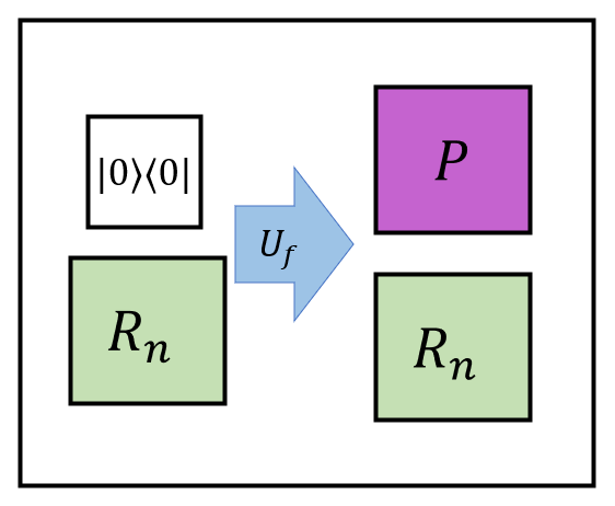
(a)

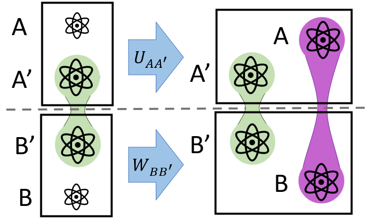
(b)

Figure 3: Comparison between embezzlement of classical distributions and quantum states. (a) The embezzlement of classical distributions happens within one lab and a local permutation of the joint computational basis. (b) The embezzling of quantum states happens across two labs where each party applies the permutation of the joint computational basis on their local halves.

Theorem 2.

For any $\varepsilon>0$ and target probability distribution $P\in\mathcal{P}(m)$, the catalyst distribution $R_{n}:=\frac{1}{H_{n}}\sum_{j=1}^{n}\frac{1}{j}\outerproduct{j}{j}$ is such that for $n>m^{1/\varepsilon}$ there exists a unitary representation of a basis relabeling $U_{f}$ of the joint distribution such that

$$F(U_{f}(R_{n}\otimes\outerproduct{0}{0})U_{f}^{\dagger},R_{n}\otimes P)\geq 1-\varepsilon\ .$$

We note the major difference between randomness and quantum embezzlement is the role of locality. In the classical case there is a single party and the distribution is not bipartite, both of which remove the notion of locality. These differences are non-trivial: one cannot construct a non-local classical equivalent of embezzling that at the same time demands that the catalyst remains decoupled as in Proposition 3, and one cannot find a quantum equivalent of the non-local classical variation that one can implement as follows from Proposition 2. As it is not central to the rest of this work, we provide an extended discussion of this nuance for the interested reader in Appendix A after the proof of Theorem 2.

IV.2 Pure State Conversion under Local Unitaries

Having established the relationship between the equivalence classes of pure states in terms of Schmidt coefficients and the probability simplex, we now show the optimal strategy for converting one pure state to another under local unitaries is simply re-labeling the Schmidt basis so the ordering of the Schmidt coeffficients is the same. This is not necessarily surprising. It is not clear what more one could do, and indeed this is the strategy that is used to implement quantum embezzlement [12]. For intuition, we quickly show the equivalent result in the classical setting first.

Proposition 7.

Let $p^{\downarrow},q^{\downarrow}\in\mathcal{P}^{\downarrow}(d)$ Then for any $i\in[d]$ and $d-k\geq k\geq 1$,

$$1\geq\sqrt{p^{\downarrow}(i)}\sqrt{q^{\downarrow}(i)}\geq\sqrt{p^{\downarrow}(i)}\sqrt{q^{\downarrow}(i+k)}\ .$$

Proof.

This just follows from the fact if $1\geq p^{\downarrow}(i)\geq p^{\downarrow}(i+1)$ and the same for $q^{\downarrow}$. ∎

Corollary 1.

Given $p,q\in\mathcal{P}(d)$,

$$\max_{\pi\in\mathcal{S}_{d}}BC(p,\pi q)=BC(p^{\downarrow},q^{\downarrow})\ ,$$

where $\mathcal{S}_{d}$ is the set of permutations on $d$ elements.

Proof.

All we are looking for is the permutation of the elements of $q$ such that $BC(p,\pi q)$ is maximized. We can apply the permutation $\sigma$ such that $\sigma P\sigma^{\dagger}=P^{\downarrow}$, the matrix representation of $p^{\downarrow}$, to both sides. By the isometric equivalence of fidelity and that permutations are group, the problem is the same. That is, we can consider

$$\max_{\pi\in\mathcal{S}_{d}}BC(p^{\downarrow},\pi q)=\max_{\pi\in\mathcal{S}_{d}}\sum_{i\in[d]}\sqrt{p^{\downarrow}(i)}\sqrt{q(\pi(i))}\ .$$

It immediately follows from Proposition 7 that the optimal $\pi$ is the one that takes $Q$ to $Q^{\downarrow}$. This completes the proof. ∎

The idea is then to lift this result to quantum states optimized over unitaries and then use this with Uhlmann’s theorem to lift to the bipartite setting with local unitaries. The main challenge is minimizing over unitaries in the lift of the previous result as now we have to deal with non-commutivity. This is done by reducing optimizing over unitaries to optimizing over permutations using the Birkhoff-von Neumann Theorem.

Lemma 3 (Birkhoff-von Neumann Theorem).

Let $d\in\mathbb{N}$. Given a linear operator $X\in\mathrm{L}(\mathbb{R}^{d})$, $X$ is bistochastic (non-negative entries such that each column and each row sums to one) if and only if there exists a probability distribution $p\in\mathcal{P}(|\mathcal{S}_{d}|)$ such that

$$X=\sum_{\pi\in\mathcal{S}_{d}}p(\pi)V_{\pi}\ ,$$

where $V_{\pi}(i,j):=\delta_{i,\pi(j)}$ are permutation matrices and $\delta_{i,j}$ is the Kronecker delta. That is, a linear operator is bistochastic if and only if it is a convex combination of permutation matrices.

Lemma 4.

Let $\rho,\sigma\in\mathrm{D}(\mathbb{C}^{d})$. Then

$$\max_{U}F(\rho,U\sigma U^{\dagger})=F(P^{\downarrow},Q^{\downarrow})\ ,$$

where $P^{\downarrow}=\sum_{i}\nu_{i}(\rho)\outerproduct{i}{i}$ and likewise for $Q^{\downarrow}$ but with respect to $\sigma$. In other words, the fidelity between $\rho$ and $\sigma$ maximized over unitaries is equal to the fidelity of their ordered eigenvalues.

Proof.

First, by the isometric invariance of fidelity (Item 2 of Proposition 1), $F(\rho,\sigma)=F(P^{\downarrow},V\sigma V^{\dagger})$ where $V$ is the unitary such that $V\rho V^{\dagger}=P^{\downarrow}=\sum_{i}\nu_{i}(\rho)\outerproduct{i}{i}$. As unitaries are closed under multiplication and conjugate transpose,

$$\max_{U}F(\rho,U\sigma U^{\dagger})=\max_{U^{\prime}}F(P^{\downarrow},U^{\prime}V\sigma V^{\dagger}{U^{\prime}}^{\dagger})$$

as the optimal $U^{\prime}=U^{\star}V^{\dagger}$ where $U^{\star}$ is the optimizer for the L.H.S. of the equality. Therefore we just define $Q\equiv V\sigma V^{\dagger}$ and focus on solving the R.H.S. for clarity. Therefore, we are interested in $\max_{U}F(P^{\downarrow},UQU^{\dagger})$.

Denote the spectral decomposition of $Q=\sum_{j}q(j)\outerproduct{\phi_{j}}{\phi_{j}}$. Note that without loss of generality, we may write $U=\sum_{j}\ket{\psi_{j}}\bra{\phi_{j}}$ for some orthonormal basis $\{\ket{\psi_{j}}\}$. Therefore, $UQU^{\dagger}=\sum_{j}q(j)\outerproduct{\psi_{j}}{\psi_{j}}$. Furthermore, define $\mathbb{P}(X):=\sum_{i}\outerproduct{i}{i}X\outerproduct{i}{i}$, which is the pinching, or dephasing, channel onto the computational basis. Then

$$\mathbb{P}(UQU^{\dagger})= \sum_{i,j}\outerproduct{i}{i}q(j)\outerproduct{\psi_{j}}{\psi_{j}}\outerproduct{i}{i}$$

$$= \sum_{i,j}q(j)|\bra{i}\ket{\psi_{j}}|^{2}\outerproduct{i}{i}\ .$$

Note that in contrast, $P^{\downarrow}$ is invariant under this pinching. Combining these points,

where the inequality is the data-processing inequality (Item 3 of Proposition 1) with the pinching channel along with the invariance of $P^{\downarrow}$ under this channel, the first equality is using the definition of fidelity (2), the second is just expanding everything, and the third is collapsing the implicit Kronecker deltas.

Now note the following trick. We can define the square matrix $A$ via its elements: $A(j,i):=|\bra{i}\ket{\psi_{j}}|^{2}$. We know $0\leq|\bra{i}\ket{\psi_{j}}|^{2}\leq 1$, $\sum_{i}|\bra{i}\ket{\psi_{j}}|^{2}=1$, and $\sum_{j}|\bra{i}\ket{j}|^{2}=1$ as $\{\ket{i}\}$ and $\{\ket{\psi_{j}}\}$ are orthonormal bases. It follows that $A$ is a bistochastic matrix by definition. Therefore, by the Birkhoff-von Neumann Theorem (Lemma 3), $A=\sum_{\pi\in\mathcal{S}_{d}}r(\pi)W_{\pi}$ where $W_{\pi}$ is the permutation matrix for $\pi$ and $r$ is a probability distribution over the permutations. Thus, plugging this back in to what we started with,

$$\max_{\left\{\ket{\psi_{j}}\right\}}\Tr[\left(\sum_{j,i}q(j)p^{\downarrow}(i)|\bra{i}\ket{\psi_{j}}|^{2}\outerproduct{i}{i}\right)^{1/2}]^{2}$$

$$= \max_{r}\Tr[\left(\sum_{j,i,\pi}q(j)p^{\downarrow}(i)r(\pi)W_{\pi}(j,i)\outerproduct{i}{i}\right)^{1/2}]^{2}\ .$$

Now note every permutation matrix is the identity matrix with columns permuted, i.e. $\pi=\begin{bmatrix}e_{\pi(0)}^{\mathrm{T}}&e_{\pi(1)}^{\mathrm{T}}&\ldots&e_{\pi(d-1)}^{\mathrm{T}}\end{bmatrix}^{\mathrm{T}}$, where $e_{i}:=\ket{i}$. It follows that

$$\sum_{\pi\in\mathcal{S}_{d}}r(\pi)W_{\pi}(j,i)$$

$$= \sum_{\pi}r(\pi)\mathbb{1}\{W_{\pi}(j,i)=1\}$$

$$= \sum_{\pi}r(\pi)\mathbb{1}\{\pi(j)=i\}=:\Pr_{r}[\pi(j)=i^{\prime}]\ ,$$

where $\mathbb{1}\{A\}$ is the indicator function for an event and the second equality is because $W(j,i)=1$ if and only if $\pi(j)=i$. We stress the final definition is a function of the choice of $r$ and $j,i$ and form a joint probability over $(j,i)$ as $\sum_{j}\Pr_{r}[\pi(j)=i]=1=\sum_{i}\Pr_{r}[\pi(j)=i]$ and every element is non-negative. This simplifies the problem to

$$\max_{r}\Tr[\left(\sum_{j,i,\pi}q(j)p^{\downarrow}(i)r(\pi)W_{\pi}(j,i)\outerproduct{i}{i}\right)^{1/2}]^{2}$$

$$= \max_{r}\left(\sum_{i}\sqrt{p^{\downarrow}(i)}\left\{\sum_{j}\sqrt{q(j)\Pr_{r}[\Pi(j)=i]}\right\}\right)^{2}\ ,$$

where we have just grouped terms and used that the operator is diagonal, so we can apply the square root entry-wise and take the sum to compute the trace.

So we want to determine the maximal distribution $r$, but we can show this is achieved by element-wise optimizing the sum. Note $\sqrt{p^{\downarrow}(1)}$ is the largest element and bounded above by $1$, so we want to multiply it by the largest value $\sum_{j}\sqrt{q(j)}\Pr_{r}[\pi(j)=i]$ can take. $\sqrt{q(j)}\leq 1$ for all $j$ and $\sum_{j}\Pr_{r}[\pi(j)=i]=1$ so the largest value this sum can take is $\max_{j}\sqrt{q(j)}$. Note if we pick a different distribution each term will be smaller than it could be by Proposition 7. This means we choose $r$ such that all non-zero probability permutations map $\text{argmax}_{j}\,q(j)$ to $1$. We then have the same problem as initially but with $\sqrt{p^{\downarrow}(2)}$ serving the largest element and $q$ not containing its largest element. Doing the argument recursively, we conclude the optimal distribution $r$ has unit probability on permutation $\sigma$ such that $\sum_{i}q(\sigma(i))=q^{\downarrow}$. Thus,

$$\max_{r}\left(\sum_{i}\sqrt{p^{\downarrow}(i)}\left\{\sum_{j}\sqrt{q(j)\Pr_{r}[\Pi(j)=i]}\right\}\right)^{2}$$

$$= \left[\sum_{i}\sqrt{p^{\downarrow}(i)}\sqrt{q^{\downarrow}(i)}\right]^{2}$$

$$= BC(p^{\downarrow},q^{\downarrow})^{2}$$

$$= F(P^{\downarrow},Q^{\downarrow}),$$

where the first equality is by the preceding explanation and the last two are using Item 5 of Proposition 1. Note this means we have established an upper bound as we used the data processing inequality at the beginning. However, this is clearly achievable by picking by the permutation unitary that maps $\sigma$ to $Q^{\downarrow}$. Thus this completes the proof. ∎

We now can use the above lemma to establish the pure state property we are actually interested in. For notational simplicity, we define the following notation:

$$F_{\mathrm{LU}}(\rho,\sigma):=\max_{U,V}F(\rho,(U\otimes V)(\sigma))\ ,$$

which is without loss of generality unitaries as we can just trivially embed the smaller dimensional state.

Theorem 5.

$$F_{\mathrm{LU}}(\ket{\psi},\ket{\phi})=F(P^{\downarrow},Q^{\downarrow})\ ,$$

where $P^{\downarrow}$ is the distribution defined by the decreasing Schmidt coefficients of $\ket{\psi}$ and likewise for $Q^{\downarrow}$ and $\ket{\phi}$. In other words, the optimal fidelity of converting $\ket{\phi}$ to $\ket{\psi}$ via local unitaries is given by the fidelity of their ordered Schmidt coefficients.

Proof.

Up to local unitaries, $\ket{\psi}=\sum_{i}\sqrt{p^{\downarrow}}\ket{i}\ket{i}$. Therefore without loss of generality, that can be taken as our target state by allowing free local unitaries on the seed state. We can take the seed state to be of the form $\ket{\phi}=\sum_{i}\sqrt{q(i)}\ket{i}\ket{i}$ by the same argument. Then by assumption, we are interested in $\max_{U,V}F(\ket{\psi},(U\otimes V)\ket{\phi})$ with the specified forms. Note

$$\Tr_{B}((U\otimes V)\outerproduct{\phi}{\phi}(U\otimes V)^{\dagger})$$

$$= \sum_{i,i^{\prime}}\sqrt{q(i)q(i^{\prime})}U\ket{i}\bra{i^{\prime}}U^{\dagger}\Tr(V\ket{i}\bra{i^{\prime}}V^{\dagger})$$

$$= \sum_{i}q(i)U\outerproduct{i}{i}U^{\dagger}=:UQU^{\dagger}.$$

Now for any unitary $U$ we define the following purification

$$\ket{w^{|U}}:= \operatorname{vec}(\sqrt{UQU^{\dagger}})$$

$$= (\overline{U}\otimes U)\operatorname{vec}(\sqrt{Q})=(\overline{U}\otimes U)\ket{\phi}\ ,$$

where we have used $\sqrt{UQU^{\dagger}}=U\sqrt{Q}U^{\dagger}$ and the vec map identity (1). Now we have

$$F(P^{\downarrow},UQU^{\dagger})= \max_{\ket{w^{\prime}}}F(\ket{\psi},\ket{w^{\prime}})$$ (6)

$$= \max_{V}F\left(\ket{\psi},(\mathbb{1}\otimes V)\ket{w^{|U}}\right)$$

$$= \max_{V}F(\psi,(\overline{U}\otimes VU)\ket{\phi})\ ,$$

where the first equality is by Uhlmann’s theorem (Lemma 1), the second is because all purifications of a given operator are unitarily equivalent on the purifying space, so there exists a $V$ such that $(\mathbb{1}\otimes V)\ket{w^{|U}}=\ket{w^{\prime}}$. The final line is just expanding the definition of $\ket{w^{|U}}$.

It follows,

$$\max_{W,V}F(\ket{\psi},(W\otimes V)\ket{\phi})$$

$$= \max_{\overline{U},V^{\prime}}F(\ket{\psi},(\overline{U}\otimes V^{\prime}U)\ket{\phi})$$

$$= \max_{\overline{U},V^{\prime}}F(\ket{\psi},(\mathbb{1}\otimes V)\ket{w^{|U}})$$

$$= \max_{U}F(P^{\downarrow},UQU^{\dagger})$$

$$= F(P^{\downarrow},Q^{\downarrow})\ ,$$

where the first equality is because unitaries are closed under multiplication and the optimizations are independent, the second and third are both by (6) for clarity, the third is because unitaries are closed under conjugation and then the final equality is by applying Lemma 4. This completes the proof. ∎

This means under local unitaries, it is efficient to compute the optimal fidelity and that in fact the optimal strategy is simply Alice and Bob re-ordering the basis so that the Schmidt coefficients are in the same relative ordering. It also follows from Item 1 of Proposition 1 that unless all the Schmidt coefficients are equal, the fidelity cannot be one under local unitary strategies.

IV.3 Pure State Conversions under Local Operations and Shared Randomness

While the previous section is nice in that it finds an efficient way of calculating the optimal conversion strategy under local unitaries, it would be natural to ask if local operations can do better than local unitaries as it is a much more general class of operations. In fact, we can see that it must do better in some cases in a trivial manner. Consider the target state $\ket{\psi}$ and the seed state $\ket{\phi}=\ket{\psi}\otimes\ket{\zeta}$ where $\ket{\zeta}$ is not product. Under local unitaries this transformation isn’t possible to arbitrary precision because of $\ket{\zeta}$, but of course in reality the parties could trace out whichever portion(s) of $\ket{\zeta}$ they hold. Thus, we need a theory of transformations under local operations.

Note that this trivial example we have given would not be resolved by local mixed unitary strategies. Indeed, we begin by noting that local mixed unitary strategies cannot ever outperform local unitary strategies.

Corollary 2.

Let $\ket{\psi}$ be the target state and $\ket{\phi}$ be the seed state and only optimize over Alice and Bob using mixed unitary channels. Then the optimal is the same as in Theorem 5.

Proof.

Letting $\mathcal{E}_{U},\mathcal{F}_{W}$ be local mixed unitary maps,

$$\max_{\mathcal{E}_{U},\mathcal{F}_{W}}F(\psi,(\mathcal{E}_{U}\otimes\mathcal{F}_{W})(\phi))$$

$$= \bra{\psi}(\mathcal{E}_{U}\otimes\mathcal{F}_{W})(\phi)\ket{\psi}$$

$$= \int_{U,W}\bra{\psi}(U\otimes W)(\phi)\ket{\psi}dU\,dW$$

$$\leq \int_{U,W}\max_{U,W}\bra{\psi}(U\otimes W)(\phi)\ket{\psi}$$

$$= \max_{U,W}\bra{\psi}(U\otimes W)(\phi)\ket{\psi}$$

$$= F(P^{\downarrow},Q^{\downarrow})\ ,$$

where the first equality is by Item 4 of Proposition 1, the second is letting the mixed unitary map be for any probability measures $dU$,$dW$ over the unitary group. The inequality is because the inner product is real and so it is lower bounded by the maximum. The second to last equality is by linearity, and the final equality is by Theorem 5. Noting that a specific choice of local unitaries is a special case of mixed unitary channels completes the proof. ∎

The above tells us that we must escape the use of unitaries to improve our bounds. Note however that in general the only maps that preserve pure states are isometries, and our results so far have been in terms of pure states, so we need to maintain this structure to build on them. For this reason, the following proof will make use of the isometric representation of quantum channels.

For notational simplicity, we define the optimal fidelity of conversion under local operations and shared randomness (LOSR) fidelity

$$F_{\mathrm{LOSR}}(\rho,\sigma):=\max_{\mu,\mathcal{E}_{\lambda},\mathcal{F}_{\lambda}}F(\rho,\int(\mathcal{E}_{\lambda}\otimes\mathcal{F}_{\lambda})(\sigma)d\mu(\lambda))\ ,$$

where $\mu$ is a probability measure over an index set for sets of local channels $\{\mathcal{E}_{\lambda}\}$ and $\{\mathcal{F}_{\lambda}\}$. Similarly, we can define optimal fidelity of conversion under local operations (LO) as

$$F_{LO}(\rho,\sigma):=\max_{\mathcal{E},\mathcal{F}}F(\rho,\mathcal{E}\otimes\mathcal{F})(\sigma))\ .$$

With these defined, we prove the following.

Theorem 6.

$$F_{LOSR}(\ket{\psi},\ket{\phi}) =F_{LO}(\ket{\psi},\ket{\phi})$$

$$=\max_{P^{\prime}\in\mathcal{P}(\Sigma)}F((P\otimes P^{\prime})^{\downarrow},Q^{\downarrow}_{\text{embed}})\ ,$$

where $|\Sigma|\leq\mathrm{SR}(\ket{\phi})\cdot\mathrm{SR}(\ket{\psi})$, $P$ is the probability distribution defined by $\ket{\psi}$’s Schmidt coefficients and likewise for $Q_{\text{embed}}$ with the Schmidt coefficients of $\ket{\phi}$ except the distribution is embedded into the joint space.

Proof.

The first equivalence follows similarly to the mixed unitary case. Clearly the class of LOSR strategies is more general than the class of LO strategies, so we just need to show LOSR is only as strong as LO here.

$$F_{\mathrm{LOSR}}(\phi,\psi)= F\left(\psi,\int(\mathcal{E}_{\lambda}\otimes\mathcal{F}_{\lambda})(\phi)d\mu(\lambda)\right)$$

$$= \int\bra{\psi}(\mathcal{E}_{\lambda}\otimes\mathcal{F}_{\lambda})(\phi)\ket{\psi}d\mu(\lambda)$$

$$\leq \int\max_{\mathcal{E},\mathcal{F}}\left[\bra{\psi}(\mathcal{E}\otimes\mathcal{F})(\phi)\ket{\psi}\right]d\mu(\lambda)$$

$$= \max_{\mathcal{E},\mathcal{F}}\bra{\psi}\mathcal{E}\otimes\mathcal{F})(\phi)\ket{\psi}$$

$$= F_{LO}(\phi,\psi)\ ,$$

where the first equality is by definition and denoting the optimizers by $\mu,\{\mathcal{E}_{\lambda}\},\{\mathcal{F}_{\lambda}\}$, the second is by linearity of the Lebesgue integral, the inequality is because $\bra{\psi}(\mathcal{E}\otimes\mathcal{F})(\phi)\ket{\psi}$ is a real number for any choice of local channels, the third equality is because $\mu$ is a probability measure that is now independent of the argumenbt of the integral, and the final equality is by definition. This proves the reduction of LOSR to LO if the target state is pure.

Next, we bound the dimension of $\Sigma$. We want to consider $\max_{\mathcal{E},\mathcal{F}}F(\psi,(\mathcal{E}\otimes\mathcal{F})(\phi))$. Without loss of generality, we assume the local spaces are ‘compressed’ such that $d_{in}:=\mathrm{SR}(\ket{\phi})$ so that $\mathcal{E},\mathcal{F}$ both act on $\mathrm{L}(\mathbb{C}^{d_{in}})$. We now show that without loss of generality we may restrict the output dimension of $\mathcal{E},\mathcal{F}$ to be $d_{out}:=\mathrm{SR}(\ket{\psi})$. This is just because we can project onto the support of the marginal of $\ket{\psi}$ on both local spaces, so we can restrict the local maps to this space. Formally, this can be seen as follows. Consider arbitrary $\mathcal{E},\mathcal{F}$ and let $\ket{\psi}=\sum_{i}\sqrt{p(i)}\ket{i}\ket{i}$. Define $\Pi_{P}:=\sum_{i:p(i)>0}$, i.e. the projector onto the support of $\Tr_{B}(\psi)=\Tr_{A}(\psi)$, where the equality is up to the change in space. Note $\mathrm{rank}(\Pi_{P})=\mathrm{Schmidt}(\psi)$. By construction, $(\Pi_{P}\otimes\Pi_{P})\ket{\psi}=\ket{\psi}$. Therefore,

$$F(\psi,(\mathcal{E}\otimes\mathcal{F})(\phi))$$

$$= \bra{\psi}(\mathcal{E}\otimes\mathcal{F})(\phi)\ket{\psi}$$

$$= \Tr[\outerproduct{\psi}{\psi}(\mathcal{E}\otimes\mathcal{F})(\phi)]$$

$$= \Tr[\psi\Pi_{P}^{\otimes 2}(\mathcal{E}\otimes\mathcal{F})(\phi)\Pi_{P}^{\otimes 2}]\ ,$$

where in the first equality we have used Item 4 of Proposition 1 and the other two use cyclicity of trace along with invariance of $\psi$ under the projector. Now we can expand,

$$\Pi_{P}^{\otimes 2}(\mathcal{E}\otimes\mathcal{F})(\phi)\Pi_{P}^{\otimes 2}$$

$$= \sum_{k,l}\Pi_{P}A_{k}\otimes\Pi_{P}B_{k}\phi A_{k}^{\dagger}\Pi_{P}\otimes B_{l}^{\dagger}\Pi_{P}$$

$$\equiv (\mathcal{E}_{\Pi}\otimes\mathcal{F}_{\Pi})(\psi)\ ,$$

where $\{A_{k}\},\{B_{l}\}$ are the Kraus operators of $\mathcal{E},\mathcal{F}$ respectively and $\mathcal{E}_{\Pi},\mathcal{F}_{\Pi}$ are CPTNI maps defined by $\{\Pi_{P}A_{k}\},\{\Pi_{P}B_{l}\}$ respectively. Note this equivalence holds as $(\Pi A_{k})^{\dagger}=A_{k}^{\dagger}\Pi_{P}$ since $\Pi_{P}^{\dagger}=\Pi_{P}$ so it is CP and it is TNI because

$$\sum_{k}(\Pi_{P}A_{k})^{\dagger}(\Pi_{P}A_{k})= \sum_{k}A_{k}^{\dagger}\Pi_{P}A_{k}$$

$$\leq \sum_{k}A_{k}^{\dagger}\mathbb{1}A_{k}=\mathbb{1}\ ,$$

where we used $\Pi_{P}^{2}=\Pi_{P}$ in the first equality, $\Pi_{P}\leq\mathbb{1}$ and that $\mathcal{E}$ is CP in the inequality, and that $\mathcal{E}$ is TP in the last inequality. An identical argument holds for $\mathcal{F}_{P}$. This proves the optimizer is achieved with CPTNI maps $\mathrm{T}(\mathrm{L}(\mathbb{C}^{d_{in}}),\mathrm{L}(\mathbb{C}^{d_{out}}))$. Finally, we can lift $\mathcal{E}_{P},\mathcal{F}_{P}$ to being CPTP, denoted $\widehat{\mathcal{E}},\widehat{\mathcal{F}}\in\mathrm{T}(\mathrm{L}(\mathbb{C}^{d_{in}}),\mathrm{L}(\mathbb{C}^{d_{out}}))$ by adding one Kraus operator, e.g. for $\mathcal{E}_{P}$ add the Kraus operator $Z\in\mathrm{L}(\mathbb{C}^{d_{in}},\mathbb{C}^{d_{out}})$ where $Z^{\dagger}Z=(\mathbb{1}-\sum_{k}A_{k}^{\dagger}\Pi A_{k})\geq 0$ which always exists by definition of the space of positive semidefinite operators. By linearity,

$$F(\psi,(\mathcal{E}\otimes\mathcal{F})\phi)= \Tr[\psi(\mathcal{E}_{\Pi}\otimes\mathcal{F}_{\Pi})(\phi)]$$

$$\leq \Tr[\psi(\widehat{\mathcal{E}}\otimes\widehat{\mathcal{F}})(\phi)]\ .$$

Therefore without loss of generality the optimal channels are $\mathcal{E},\mathcal{F}\in\mathrm{C}(\mathbb{C}^{d_{in}},\mathbb{C}^{d_{out}})$. Note this means that $\mathrm{Rank}(J_{\mathcal{E}})\leq d_{in}d_{out}$ and likewise for $J_{\mathcal{F}}$.

We now derive the equation using the isometric representation of the channel.

$$\max_{\mathcal{E},\mathcal{F}}F(\psi,(\mathcal{E}\otimes\mathcal{F})(\phi))$$

$$= \langle\psi,(\mathcal{E}\otimes\mathcal{F})(\phi)\rangle$$

$$= \max_{V_{1},V_{2},\ket{\zeta}}\left|\bra{\psi}\bra{\zeta}(V_{1}\otimes V_{2})\ket{\phi}\right|^{2}$$

$$= \max_{U_{1},U_{2},\ket{\zeta}}\left|\bra{\psi}\bra{\zeta}(U_{1}\otimes U_{2})\ket{\phi}\ket{0}_{E_{1}}\ket{0}_{E_{2}}\right|^{2}$$

$$= \max_{U_{1}^{\prime},U_{2}^{\prime},\ket{\zeta_{p^{\prime}}}}\left|\bra{\psi}\bra{\zeta_{p^{\prime}}}(U_{1}^{\prime}\otimes U_{2}^{\prime})\ket{\phi}\ket{0}_{E_{1}}\ket{0}_{E_{2}}\right|$$

$$= \max_{P^{\prime}}F((P\otimes P^{\prime})^{\downarrow},Q^{\downarrow}_{\mathrm{embed}})\ ,$$

where the second line is because there exists an isometric representation of each channel which means $(V_{1}\otimes V_{2})(\phi)$ is a pure state, so we can apply Uhlmman’s theorem to find a purification of $\ket{\psi}$ that saturates the bound, but as $\ket{\psi}$ is already pure, any purification will be a product state. The third line is because we can always convert an isometry into a unitary on the appropriately large space. The fourth line means that $\zeta_{p^{\prime}}=\sum_{i^{\prime}}\sqrt{p^{\prime}(i)}\ket{i}\ket{i}$, which can always be achieved by local unitaries on the $E_{1}$ and $E_{2}$ spaces, which result on new unitaries on the other side but the same maximum. The final equality is just using Theorem 5 and we write $Q_{\mathrm{embed}}$ to stress it is defined over the whole alphabet. Lastly, as we established bounds on the ranks of the local maps Choi matrices, we have bounds $E_{1},E_{2}\leq d_{in}d_{out}$, which justifies the maximum and tells us how large of a system we have to consider in the statement of the theorem. ∎

It is useful to see how this result works. It in effect shows the following equivalence of conversion when measured under fidelity

$$\ket{\phi}\xrightarrow[LO]{}\ket{\psi}\,=\,\max_{\ket{\zeta}}\,\left[\ket{\phi}\xrightarrow[LU]{}\ket{\psi}\otimes\ket{\zeta}\right]\ ,$$

which can be viewed both by proof and via intuition as a special case of the isometric representation of a channel. Moreover, it is easy to see in this form how it handles our motivating example. Indeed, if the target state is $\ket{\psi}$ and the seed state is $\ket{\psi}\otimes\ket{\zeta}$, then clearly the maximizer is chosen by the ancillary state being $\ket{\zeta}$ and the local unitaries being trivial.

IV.4 Relation between LO and LU Strategies

The natural question given the previous theorems is if we can better understand the relationship between LO and LU strategies. We first show that LU and LO strategies are equivalent when either the target or the seed state is a two qubit state.

IV.4.1 LU and LO Equivalence for Two-Qubit Seed or Target State

Proposition 8.

Consider entangled two qubit seed state $\ket{\phi}\in\mathbb{C}^{2}\otimes\mathbb{C}^{2}$. Let the target entangled state be $\ket{\psi}\in\mathbb{C}^{d}\otimes\mathbb{C}^{d^{\prime}}$. Then the optimal non-communicative strategy is the local unitary strategy.

Proof.

Without loss of generality, $q^{\downarrow}=(q,1-q)$ where $q\geq 1/2$ and $p^{\downarrow}=(p(1),p(2),...)$. Then the optimal local unitary strategy is $\sqrt{qp(1)}+\sqrt{(1-q)p(2)}$. For any $P^{\prime}$ we can write $(p^{\prime})^{\downarrow}=(p^{\prime}(1),p^{\prime}(2),...)$. The optimal CPTP strategy (up to a square) is of the form

$$\sqrt{qp(1)p^{\prime}(1)}+\sqrt{(1-q)\max\{p(1)p^{\prime}(2),p(2)p^{\prime}(1)\}}\ .$$

These values can only increase by assuming $p^{\prime}$ has two outcomes, so let us assume so without loss of generality and parameterize the distribution by $p^{\prime}\in[1/2,1]$ to obtain

$$\sqrt{qp(1)p^{\prime}}+\sqrt{(1-q)\max\{p(1)(1-p^{\prime}),p(2)p^{\prime}\}}\ .$$

Moreover note $p(2)p^{\prime}<p(2)$ unless $p^{\prime}=1$, which is equivalent to the LU strategy, so the second entry in the maximization would be lower than the LU setting. Therefore, we focus on the remaining case. We are specifically interested in when the following strict inequality holds:

$$\sqrt{qp(1)p^{\prime}}+\sqrt{(1-q)p(1)(1-p^{\prime})}$$

$$\hskip 56.9055pt>\sqrt{qp(1)}+\sqrt{(1-q)p(2)}$$

$$\Leftrightarrow\, g(p^{\prime}):=\sqrt{qp(1)}(\sqrt{p^{\prime}}-1)$$

$$\hskip 42.67912pt+\sqrt{1-q}(\sqrt{p(1)(1-p^{\prime})}$$

$$\hskip 113.81102pt-\sqrt{p(2)})>0\ .$$

Then $\frac{d}{dp^{\prime}}g(p^{\prime})=\frac{\sqrt{qp(1)}}{2\sqrt{p^{\prime}}}+\frac{\sqrt{p(1)(1-q)}}{2\sqrt{1-p^{\prime}}}$. It follows,

$$\frac{\sqrt{qp(1)}\sqrt{1-p^{\prime}}}{2\sqrt{p^{\prime}}\sqrt{1-p^{\prime}}}+\frac{\sqrt{p^{\prime}}\sqrt{p(1)(1-q)}}{2\sqrt{1-p^{\prime}}\sqrt{p^{\prime}}}\geq 0$$

$$\Leftrightarrow \sqrt{qp(1)}\sqrt{1-p^{\prime}}+\sqrt{p^{\prime}}\sqrt{p(1)(1-q)}\geq 0$$

$$\Leftrightarrow \sqrt{q}\sqrt{1-p^{\prime}}+\sqrt{p^{\prime}}\sqrt{(1-q)}\geq 0$$

$$\Leftrightarrow \sqrt{F}(Q^{\downarrow},P^{\prime\downarrow})\geq 0\ ,$$

where the first line is multiplying to get identical denominators, the second line is multiplying by the denominator, the third is dividing out $p(1)$, and the final is by the definition of square root fidelity. Note the final inequality will always hold strictly unless $q\in\{0,1\}$, i.e. the state is a product state, by Item 1 of Proposition 1. If $q\in\{0,1\}$, then the state is a product state which would contradict that we assume the state is entangled. Therefore, in our setting, $g(p^{\prime})$ only increases over its interval, $p^{\prime}\in[0,1]$. Thus, the optimal choice of $p^{\prime}$ is $p^{\prime}=1$, but in this case the value is $\sqrt{qp(1)}\leq\sqrt{qp(1)}+\sqrt{(1-q)p(2)}$, i.e. the optimal choice is lower bounding the optimal local unitary strategy. It follows this is never optimal. This completes the proof. ∎

Proposition 9.

Consider entangled two qubit target state $\ket{\psi}\in\mathbb{C}^{2}\otimes\mathbb{C}^{2}$ and any seed state $\ket{\phi}\in\mathbb{C}^{d}\otimes\mathbb{C}^{d^{\prime}}$. The optimal non-communicative strategy is the local unitary strategy.

Proof.

The proof is basically the same as for the two qubit seed case. Without loss of generality, $p^{\downarrow}=(p,1-p)$. We can re-order $\ket{\phi}$ such that it is $q^{\downarrow}=(q(1),q(2),...)$. The optimal CPTP strategy (up to a square) is of the form

$$\sqrt{q(1)p^{\prime}(1)p}+\sqrt{q(2)\max\{p^{\prime}(1)(1-p),p^{\prime}(2)p\}}\ .$$

This sum can only increase if $p^{\prime}(1)+p^{\prime}(2)=1$, so we can parameterize the distribution by $p^{\prime}\in[1/2,1]$ to obtain

$$\sqrt{q(1)p^{\prime}p}+\sqrt{q(2)\max\{p^{\prime}(1-p),(1-p^{\prime})p\}}\ .$$

Note that $p^{\prime}(1-p)<(1-p)$ unless $p^{\prime}=1$. If $p^{\prime}=1$, this is the LU strategy, if $p^{\prime}<1$, then this is worse than an LU strategy. Therefore, we only care about the other maximization case. That is, we are interested in when $p\in[1/2,1)$ and the following strict inequality holds:

$$\sqrt{q(1)p^{\prime}p}+\sqrt{q(2)p(1-p^{\prime})}$$

$$\hskip 56.9055pt>\sqrt{q(1)p}+\sqrt{q(2)(1-p)}\ .$$

However, $\sqrt{q(1)p^{\prime}p}<\sqrt{q(1)p}$ and $\sqrt{q(2)p(1-p^{\prime})}<\sqrt{q(2)(1-p)}$ as $p^{\prime}\in[1/2,1)$. Therefore this strict inequality can never hold. Therefore the optimal strategy is always the LU strategy. This completes the proof. ∎

IV.4.2 LU and LO Inequivalence for States with Schmidt Rank Greater than Two

If there is equivalence for two qubit seed or target states, it is natural to ask if this property persists. One might expect that this is a special property of qubit systems as are found throughout quantum information science results. Indeed, generally this property does not hold, which we will prove via example.

Theorem 7.

For seed and target state with Schmidt rank $\geq 3$, the optimal LO strategy may be better than the optimal LU strategy.

Proof.

We construct an example for Schmidt rank $3$. By continuity of the fidelity, one can embed the target and seed in bigger spaces with arbitrarily small perturbations for it to hold in higher dimensions, which is why this is sufficient. Consider target state $\ket{\psi}=0.85\ket{00}+0.08\ket{11}+0.07\ket{22}$ and seed state $\ket{\phi}=0.45(\ket{00}+\ket{11})+0.1\ket{22}$. Then, the optimal LU strategy fidelity is

$$F(P^{\downarrow},Q^{\downarrow})$$

$$= \left(\sqrt{0.45}(\sqrt{0.85}+\sqrt{0.08})+\sqrt{0.1(0.07)}\right)^{2}$$

$$< 0.796\ .$$

In contrast, if we consider $P^{\prime}=[0.55,0.28,0.17]$, then

$$F((P\otimes P^{\prime})^{\downarrow},Q^{\downarrow})$$

$$= \left(\sqrt{0.45}\sqrt{0.4675}+\sqrt{0.45}\sqrt{0.238}+\sqrt{0.1}\sqrt{0.1445}\right)^{2}$$

$$> 0.82\ .$$

As we maximize over $P^{\prime}$, the optimal LO strategy achieves a value that is strictly above the LU strategy. This completes the proof. ∎

IV.5 Inefficiency of Optimal LOSR Fidelity and Computable Upper Bounds

In the above we have constructed an example where the local operations strategy outperforms the local unitary strategy (though we have not shown what the strategy itself is). A natural question would then be how easy it is to solve for the optimal fidelity value or even a bound. By Theorem 5, we can conclude the optimal local unitary strategy is polynomial time to solve as all one needs to do is sort the Schmidt coefficients and calculate the fidelity. Indeed, one could solve for the ordering of the Schmidt coefficients using the linear program for sorting a vector.

In contrast, for optimizing LO strategies, we have no such luck. In effect this is because there are two things to optimize over at once. Indeed, recall

$$F_{LO}(\ket{\psi},\ket{\phi})=\max_{P^{\prime}\in\mathcal{P}(\Sigma)}F((P\otimes P^{\prime})^{\downarrow},Q^{\downarrow})\ .$$

Then the problem is that one must first tensor $P$ onto variable $P^{\prime}$ and then re-order the vector. One cannot even in general order an optimization variable, which we will refer to as ‘sorting,’ as sorting is in general non-convex. In sorting a vector using a linear program, one relaxes to bistochastic channels and considers a linear function so that the optimizer is an extreme point which by the Birkhoff von Neumann theorem is a specific permutation. However, we are many levels of involvement above that: we want the distribution $P^{\prime}$ such that its product distribution $P\otimes P^{\prime}$ when sorted optimizes the fidelity with $Q^{\downarrow}$. Therefore, we need to optimize over $P^{\prime}$ and the permutation at the same time. It’s not clear that we can actually relax to bistochastic strategies because of the joint concavity of fidelity. That is to say, for any bistochastic channel $\mathcal{E}$,

$$F(\mathcal{E}(P\otimes P^{\prime}),Q^{\downarrow})= F(\sum_{\pi}r(\pi)V_{\pi}(P\otimes P^{\prime}),Q^{\downarrow})$$

$$\geq \sum_{\pi}F(r(\pi)V_{\pi}(P\otimes P^{\prime}),r(\pi)Q^{\downarrow})$$

$$= \sum_{\pi}r(\pi)F(V_{\pi}(P\otimes P^{\prime}),Q^{\downarrow})\ ,$$

where the first line is Birkhoff-von Neumann theorem, the second is joint concavity using $Q^{\downarrow}=\sum_{\pi}r(\pi)Q^{\downarrow}$ as $r$ is a probability distribution, and the last line is because $F(\lambda P,Q)=\lambda F(P,Q)=F(P,\lambda Q)$. Thus any bistochastic channel may strictly do better than the average of its extreme points. Moreover, even if we could optimize over bistochastic channels, we would have a non-convex objective function as the bistochastic channel, an optimization variable, would be applied to $P\otimes P^{\prime}$ which is also partially an optimization variable.

Given the above, it seems likely the best option if one were to try and find a (near) optimum would be to use gradient descent from random initial $P^{\prime}$, realizing it will only work locally and will break down at ‘kinks’ where the ordering changes. Otherwise more sophisticated non-convex optimization techniques might be used.

Computable Upper Bound Methods

Perhaps even worse than our inability to calculate the exact fidelity, is that it is not clear in general how to determine good bounds. Certainly we have the following result.

Theorem 8.

Unless the target state is $\ket{\psi}=\ket{\phi}\otimes\ket{\zeta}$ where $\ket{\phi}$ is the seed state, there exists $\varepsilon>0$ such that there does not exist local operations that will take $\ket{\phi}$ to $\ket{\psi}$.

Proof.

This follows from Theorem 6 along with Item 1 of Proposition 1. ∎

The above theorem, while derived from a very different strategy than Proposition 2, does not seem to give us much more information as to at what point communication is necessary. What we would want to efficiently improve this would be to establish upper bounds on the equation given in Theorem 6 that have a closed form that does not depend on $P^{\prime}$. One option is to use the data processing inequality for fidelity. This can be seen in the following proposition.

Proposition 10.

Consider target state $\ket{\psi}$ and seed state $\ket{\phi}$ with corresponding Schmidt distributions $p,q$ respectively. If $p_{\max}\leq q_{\max}$, then

$$F_{LO}(\ket{\psi},\ket{\phi})\leq F(\overline{p},\overline{q})\ ,$$

where $\overline{p}=p_{\max}\outerproduct{0}{0}+(1-p_{\max})\outerproduct{1}{1}$ and likewise for $\overline{q}$.

Proof.

Without loss of generality let $d$ be the maximum local dimension. Let $\mathcal{E}(\cdot)=\outerproduct{0}{0}\cdot\outerproduct{0}{0}+\sum_{i\in\{1,...,d-1\}}\ket{1}\bra{i}\cdot\ket{i}\bra{1}$. That is, $\mathcal{E}$ coarse-grains a probability distribution to the Bernoulli distribution with its first element untouched and the sum of all the others as the other outcome. Then using data processing of fidelity (Item 3 of Proposition 1),

$$\max_{P^{\prime}\in\mathcal{P}(\Sigma)}F((P\otimes P^{\prime})^{\downarrow},Q^{\downarrow})$$

$$\leq \max_{P^{\prime}\in\mathcal{P}(\Sigma)}F(\mathcal{E}((P\otimes P^{\prime})^{\downarrow}),\mathcal{E}(Q^{\downarrow}))$$

$$= \max_{p^{\prime}\in[0,1]}F\left(\widetilde{P}(p^{\prime}),\mathcal{E}(Q^{\downarrow})\right)\ ,$$

where $\widetilde{P}(p^{\prime}):=p_{\max}p^{\prime}\outerproduct{0}{0}+(1-p_{\max}p^{\prime})\outerproduct{1}{1}$ and $\mathcal{E}(Q^{\downarrow})=q_{\max}\outerproduct{0}{0}-(1-q_{\max})\outerproduct{1}{1}$. Now note that by assumption $p_{\max}\leq q_{\max}$. As the fidelity will only decrease as $p_{\max}p^{\prime}$ moves away from $q_{\max}$, the optimal choice is $p^{\prime}=1$. This completes the proof. ∎

The problem with the above bound is that there will be cases where $p_{\max}>q_{\max}$. Why the inequality in the other direction was required was to know for a fact what element of $p$ was relevant, namely $p_{\max}$ and that any choice of $p^{\prime}\neq 1$ would be sub-optimal. In general this strategy would require $q^{\downarrow}(j)$ is sufficiently large relative to $p^{\downarrow}(j)$. This can be determined in some cases. Here we provide a simple example.

Example 3.

Let

$$p^{\downarrow}=[3/4,1/8,1/8]^{\mathrm{T}}\quad q^{\downarrow}=[1/2,1/2]^{\mathrm{T}}\ .$$

Then $(p\otimes p^{\prime})^{\downarrow}[1:2]=p^{\prime}(1)[3/4,1/8]^{\mathrm{T}}$, and so we can coarse-grain on the second element to obtain $\overline{P}(p^{\prime})=1/8p^{\prime}\outerproduct{0}{0}+(1-1/8p^{\prime})\outerproduct{1}{1}$ and $\overline{Q}=Q^{\downarrow}$. Then as $1/8p^{\prime}<1/2$, the upper bound is $F(\frac{1}{8}\outerproduct{0}{0}+\frac{7}{8}\outerproduct{1}{1},\frac{1}{2}\mathbb{1})\approx 0.83$.

The above shows that while data processing can be sufficient in certain cases, it does not provide an easy general method. Another common alternative in quantum information theory is semidefinite relaxations of optimization problems because semidefinite programs are efficient to evaluate. In Appendix B, we establish the following upper bound and show it may be expressed as a semidefinite program, which, as everything is in terms of probability distributions, is due to the non-linearity of fidelity and nothing particularly quantum.

Theorem 9.

Consider target state $\ket{\psi}$ and seed state $\ket{\phi}$. Let $\mathrm{SR}(\psi)=d$ and $\mathrm{SR}(\phi)=d^{\prime}$. Define $A=\mathbb{C}^{d}$, $B=\mathbb{C}^{d\cdot d^{\prime}}$. Then,

$$F_{\mathrm{LOSR}}(\ket{\psi},\ket{\phi})\leq\max \;F(R,Q^{\downarrow}_{\text{embed}})$$ (7)

$$\mathrm{s.t.} \;\Tr_{B}[R]=P^{\downarrow}$$

$$\;R\in\mathcal{P}^{\downarrow}(d^{2}\cdot d^{\prime})\ ,$$

where $P$ and $Q$ are the distributions defined by $\ket{\psi}$ and $\ket{\phi}$’s Schmidt coefficients respectively. Moreover, this admits the following simple semidefinite program over the reals:

$$\max \sum_{i\in[d^{2}\cdot d^{\prime}]}x(i)$$ (8)

s.t. $$\;\begin{pmatrix}\text{diag}(r)&\text{diag}(x)\\ \text{diag}(x)&\text{diag}(q^{\downarrow}_{\text{embed}})\end{pmatrix}\succeq 0$$

$$\Tr_{B}[\text{diag}(r)]=P^{\downarrow}$$

$$r\in\mathcal{P}^{\downarrow}([d^{2}\cdot d])$$

$$x\in\mathbb{R}^{d^{2}\cdot d^{\prime}}\ ,$$

Physically, this relaxation may be seen as relaxing the isometric representation of the optimal LOSR strategy to one where one allows the ancillary environment start off entangled with the local system. Mathematically, this is not too loose because we require this entangled pure state has a notion of “local Schmidt coefficients” that pertain to the original target state, although this physically does not seem to have a clean interpretation. Nonetheless, we can see that (7) will not achieve unity unless there exists a joint distribution $Q=R$, which would require $Q^{\downarrow}_{\text{embed}}$ to have $P^{\downarrow}$ as it’s marginal, which seems highly restrictive. Therefore, (7) should provide an upper bound that is non-trivial.

V Many Copy Pure State Conversion with Zero Communication

Having established what happens for single copies, we consider many copies. We provide two motivations for doing this. First, we note that it’s not clear what the limiting behaviour will be even in the LU setting. A reader may recall from other works that the fidelity is multiplicative so if $F(P,Q)<1$, then $\lim_{n\to\infty}F(P^{\otimes n},Q^{\otimes n})=\lim_{n\to\infty}F(P,Q)^{n}\to 0$. However, we lose the multiplicativity as we are considering $\lim_{n\to\infty}F((P^{\otimes n})^{\downarrow},(Q^{\otimes n})^{\downarrow})$. This issue is further aggravated if we consider local operations and the ancillary variable.

The second motivation is that what was initially considered in the literature, albeit with LOCC [23], was the conversion of many copies of states. A particular focus in the referenced work and subsequent ones is the case where either the target or seed state is the maximally entangled state, known as distillation and dilution respectively. With LOCC, we know there are ‘rates’ in the conversions. By [6] along with previous results in this work, we would not expect there to be non-negative rates without the communication assuming the error is required to be vanishing, i.e. $\varepsilon\to 0$.

In this section we establish convex optimization problems for dilution and distillation in the zero communication setting. These results are established in terms of the not-actually-a-norm $\|\cdot\|_{(k,1/2)}$, which we remind the reader is the $(k,p)-$norms extended to $p<1$ introduced in Section III with the choice of $p=1/2$. We also look at the limiting behaviour as the number of copies grows. In particular, we find a closed form when trying to convert $n-$fold two qubit states to a different $n-$fold two qubit state. Moreover, we prove the fidelity goes to zero in this case. We discuss the extension of this to entangled states with larger Schmidt rank.

V.0.1 Dilution Under Local Operations

We begin by determining the limits of dilution. For intuition, we begin with local unitaries where there is no optimization. Recall that the Schmidt coefficients of the maximally entangled state are all $\sqrt{d^{-1}}$, so they correspond to the maximally mixed distribution under our bijection between Schmidt coefficients and probability distributions.

Proposition 11.

For local unitary strategies the optimal dilution fidelity is given by

$$F_{LU}\left(\ket{\psi},\ket{\Phi^{+}_{d}}^{\otimes n}\right)=d^{-n}\left\|P\right\|_{(d^{n},1/2)}\ .$$

Proof.

Generally, if $\ket{\psi}\neq\ket{\Phi^{+}_{d}}$,

$$1> F(P^{\downarrow},\pi_{d}^{\otimes n})^{\downarrow})$$

$$= F(P^{\downarrow},\pi_{d}^{\otimes n})$$

$$= \left[d^{-n/2}\sum_{i\in[d^{n}]}\sqrt{P^{\downarrow}(i)}\right]^{2}$$

$$= d^{-n}\left[\sum_{i\in[d^{n}]}\sqrt{P^{\downarrow}(i)}\right]^{2}$$

$$= d^{-n}\|P\|_{(d^{n},1/2)}\ ,$$

where the first equality is because $\pi^{\otimes n}_{d}$ is invariant under ordering, the second is using the definition of fidelity and that $\pi^{\otimes n}_{d}$ has uniform coefficients, and the final equality is the definition of the $(k,p)-$norms. In particular note we have dropped the sorting. ∎

We remark we could have set $\ket{\phi}=\ket{\phi^{\prime}}^{\otimes m}$ to get a tradeoff, but this does not seem to provide any insight.

Just as in the one-shot setting, we know the above result isn’t as useful in general because it can’t throw out resources, so we now present the general result.

Proposition 12.

The optimal fidelity of converting $n$ $d-$local dimensional EPR pairs to $\ket{\psi}$ under local operations is given by

$$F_{LO}(\ket{\psi},\ket{\Phi^{+}_{d}}^{\otimes n})=d^{-n}\max_{P^{\prime}\in\mathcal{P}(\Sigma)}\|(P\otimes P^{\prime})\|_{(d^{n},1/2)}\ ,$$

where $\|\cdot\|_{(k,p)}$ is $(k,p)-$norm generalized to $p\geq 0$. Moreover, for fixed $n$, this is a convex optimization problem.

Proof.

Starting from the result of Theorem 6,

$$\max_{P^{\prime}\in\mathcal{P}(\Sigma)}F((P\otimes P^{\prime})^{\downarrow},(\pi_{d}^{\otimes n})^{\downarrow})$$

$$= \max_{P^{\prime}\in\mathcal{P}(\Sigma)}F((P\otimes P^{\prime})^{\downarrow},\pi_{d}^{\otimes n})$$

$$= \left[\frac{1}{d^{n/2}}\max_{P^{\prime}\in\mathcal{P}(\Sigma)}\sum_{i\in[d^{n}]}\sqrt{(P\otimes P^{\prime})^{\downarrow}(i)}\right]^{2}\quad(\star)$$

$$= \frac{1}{d^{n}}\max_{P^{\prime}\in\mathcal{P}(\Sigma)}\|P\otimes P^{\prime}\|_{(d^{n},1/2)}\ ,$$

the first inequality is invariance of $\pi_{d}^{\otimes n}$ under sorting, the second is definition of fidelity and that each element of $\pi_{d}^{\otimes n}$ is the same, the last is the definition of $(k,p)$-norm extended to $p\geq 0$.

To show this is a convex optimization problem, note that $\Phi_{P}(\cdot):=P\otimes\cdot$ is linear, $-\sqrt{\cdot}$ is operator convex, and the sum of the $k$ largest eigenvalues of a PSD $P$, which we will denote $\Sigma_{k}(P)$ is convex. Thus, starting from $(\star)$,

$$\left[d^{-n/2}\max_{P^{\prime}\in\mathcal{P}(\Sigma)}\sum_{i\in[d^{n}]}\sqrt{P\otimes P^{\prime}}^{\downarrow}(i)\right]^{2}$$

$$= \left[-d^{-n/2}\min_{P^{\prime}\in\mathcal{P}(\Sigma)}{{\Sigma}}_{d^{n}}\left(-\sqrt{\Phi_{P}(P^{\prime})}\right)\right]^{2}\ ,$$

where we have used $\max_{x\in\mathcal{C}}f(x)=-\min_{x\in\mathcal{C}}-f(x)$ and our definitions. Then ignoring the $-d^{-n/2}$ factor and the square, the optimization problem is over the probability simplex, which is a convex subset of the positive semidefinite matrices, and the objective function is convex over the positive semidefinite cone as $-\sqrt{\Phi_{P}(\cdot)}$ is operator convex and $\Sigma_{d^{n}}$ is a convex function over the space of Hermitian operators. this completes the proof. ∎

Unfortunately, while this gives computable bounds, it is not clear how one could determine the optimal value analytically.

V.0.2 Distillation Under Local Operations

We now present the same results in the distillation case, where we take some state to many EPR states. For completeness, we state the local unitaries case.

Proposition 13.

The fidelity of distillation under local unitaries and zero communication is given by

$$F_{LU}(\ket{\Phi^{+}_{d}}^{\otimes m},\ket{\psi}^{\otimes n})=d^{-m}\|P^{\otimes n}\|_{|S|,1/2}\ ,$$

where $S=[\min\{d^{m},\mathrm{rank}(P)^{n}\}]$.

Proof.

The proof is effectively identical to the dilution case by symmetry of the fidelity. ∎

In contrast to the local unitary case, the symmetry is broken when one considers local operations.

Theorem 10.

For fixed $d,m,n$ the optimal fidelity for dilution under local operations is given by

$$F_{LO}(\ket{\Phi^{+}_{d}}^{\otimes m},\ket{\psi}^{\otimes n})$$

$$= d^{-m}\left[\min_{P^{\prime}\in\mathcal{P}^{\downarrow}(\Sigma)}-\sum_{i\in\mathcal{I}}\alpha_{i}\sqrt{p^{\prime}(i)}\right]^{2}\ ,$$

where $\mathcal{P}^{\downarrow}(\Sigma)$ is the set of decreasing distributions as defined in Section III, $\mathcal{I}\equiv[\lceil\operatorname{rank}(P)^{n}/d^{m}\rceil]$, and $\alpha_{i}:=\sum_{j\in[(i-1)d^{m}:\min\{i\cdot d^{m},\operatorname{rank}(P)^{n}\}]}\sqrt{p^{\downarrow}_{n}(i)}$. Note the minimization is a convex optimization program.

Proof.

Yet again, we use the square root fidelity and then take the square at the end. Then, using Theorem 6, we have

$$F_{LO}((\Phi^{+}_{d})^{\otimes m},\psi^{\otimes n})$$

$$= \max_{P^{\prime}\in\mathcal{P}(\Sigma)}F((\pi_{d}^{\otimes m}\otimes P^{\prime})^{\downarrow},(P^{\otimes n})^{\downarrow})$$

$$= \left[\max_{P^{\prime}\in\mathcal{P}(\Sigma)}\sum_{i\in S}\sqrt{(\pi^{\otimes m}_{d}\otimes p^{\prime})^{\downarrow}(i)}\sqrt{p_{n}^{\downarrow}(i)}\right]^{2}\ .$$

Next, note

$$(\pi^{\otimes m}_{d}\otimes P^{\prime})^{\downarrow}=d^{-m/2}\sum_{i^{\prime}\in\Sigma}p^{\downarrow}(i^{\prime})\mathbb{1}_{\mathbb{C}^{d^{m}}}\ ,$$

where we have just used that $\pi_{d}^{\otimes m}$ is invariant under ordering. It follows that if we let $\mathcal{I}\equiv[\lceil\operatorname{rank}(P)^{n}/d^{m}\rceil]$, we can rewrite,

$$F_{LO}((\Phi^{+}_{d})^{\otimes m},\psi^{\otimes n})$$

$$= d^{-m}\Bigg{[}\max_{P^{\prime}\in\mathcal{P}(\Sigma)}\sum_{i\in\mathcal{I}}\sqrt{(p^{\prime})^{\downarrow}(i)}$$

$$\hskip 42.67912pt\cdot\sum_{j\in[(i-1)d^{m}:\min\{i\cdot d^{m},\operatorname{rank}(P)^{n}\}]}\sqrt{p^{\downarrow}_{n}(i)}\Bigg{]}^{2}\ .$$

Now first define $\alpha_{i}:=\sum_{j\in[(i-1)d^{m}:\min\{i\cdot d^{m},\operatorname{rank}(P)^{n}\}]}\sqrt{p^{\downarrow}_{n}(i)}$ as these coefficients may be pre-computed. Second, note that the probability simplex restricted to descending distributions, $\mathcal{P}^{\downarrow}(\Sigma)$ is itself convex as $r_{\lambda}^{\downarrow}:=\lambda p^{\downarrow}+(1-\lambda)q^{\downarrow}$ satisfies

$$\lambda p^{\downarrow}(i)+(1-\lambda)q^{\downarrow}(i)\geq\lambda p^{\downarrow}(i+1)+(1-\lambda)q^{\downarrow}(i)\ ,$$

for all $i\in[|r|]$. Thus we have,

$$F_{LO}(\ket{\Phi^{+}_{d}}^{\otimes m},\ket{\psi}^{\otimes n})$$

$$= \Bigg{[}-d^{-m}\min_{P^{\prime}\in\mathcal{P}^{\downarrow}(\Sigma)}-\sum_{i\in\mathcal{I}}\alpha_{i}\sqrt{p^{\prime}(i)}\Bigg{]}^{2}\ .$$

The minimization is a convex optimization problem because if we consider $f(p^{\prime}):=-\sum_{i}\alpha_{i}\sqrt{p^{\prime}(i)}$, then its Hessian is $\nabla^{2}f=\sum_{i}[\alpha_{i}/4p^{\prime}(i)^{-3/2}]\outerproduct{i}{i}$, which is positive semidefinite on the interior of the probability simplex (i.e. when $p^{\prime}(i)>0$ for all $i$). This completes the proof. ∎

V.0.3 Two Qubit Setting

We have now seen that even in the basic dilution and distillation setting, while we can determine convex optimization programs, we can’t seem to get clean analytic results. In this section we consider an even more tractable setting to attempt to resolve this: many copy two-qubit seed and target states. We show in this setting under certain assumptions the local unitary strategy is optimal and lobby this to show in particular that the optimal fidelity of converting $n$ copies of $\ket{\phi}$ to $n$ copies $\ket{\psi}$ goes to zero as $n$ goes to infinity. We note that this setting is more manageable because we effectively only have to reason about Bernoulli distributions.

Lemma 11.

Given Bernoulli distribution $P=p\outerproduct{0}{0}+(1-p)\outerproduct{1}{1}$, then $P^{\otimes n}$ is such that the sequence $x^{n}$ with $(n-k)$ zeros has probability $p^{n-k}(1-p)^{k}$. Moreover, there are $\binom{n}{k}$ sequences with probability $p^{k}(1-p)^{n-k}$ and the same for $p^{n-k}(1-p)^{k}$.

Proof.

The claim that $x^{n}$ with $(n-k)$ zeros has probability $p^{n-k}(1-p)^{k}$ is straightforward. The second point actually just follows from the fact there are $\binom{n}{k}$ sequences with $k$ zeros, which could be proven by induction in a straightforward manner. ∎

We can now use the above lemma along with Theorem 5 to get the optimal LU fidelity as a function of the number of copies $n$.

Corollary 3.

Consider entangled states $\ket{\psi},\ket{\phi}\in\mathbb{C}^{2}\otimes\mathbb{C}^{2}$. Then,

$$F_{LU}(\psi^{\otimes n},\phi^{\otimes n})$$

$$\hskip 14.22636pt=\sum_{k\in[n]}\binom{n}{k}(pq)^{(n-k)/2}((1-p)(1-q))^{k/2}\ .$$

Proof.

By Theorem 5 we can reduce to the Bernoulli distributions from the Schmidt coefficients, $\ket{\psi}^{\otimes n}\mapsto P^{\otimes n}$, $\ket{\phi}^{\otimes n}\mapsto Q^{\otimes n}$. Since these are Bernoulli distributions, if we assume without loss of generality $p\geq(1-p)$, we can order the probabilities simply by the exponent, e.g. $p^{j-k}(1-p)^{k}\geq p^{j-k-k^{\prime}}(1-p)^{k+k^{\prime}}$ for any $0\leq k^{\prime}\leq j-k$. Moreover, the cardinality of each set of sequences will be the same for both $P^{\otimes n}$ and $Q^{\otimes n}$ because $\ket{\psi},\ket{\phi}$ are only entangled if their Schmidt rank is two. Therefore,

$$F((P^{\otimes n})^{\downarrow},(Q^{\otimes n})^{\downarrow})$$

$$= \sum_{k\in[n]}\binom{n}{k}(pq)^{(n-k)/2}((1-p)(1-q))^{k/2}\$$

where the sum is over the number of zeros in the string, the cardinality was proven in the previous lemma, and the last term is just a re-writing of $\sqrt{p^{n-k}(1-p)^{k}}\sqrt{q^{n-k}(1-q)^{k}}$. ∎

We note it is straightforward to generalize the above result to the case where you have the number of states differs between the seed and the target, but the form would be ugly as one would need to count how many sequences of a given probability there are and keep track of this in the sum. Indeed at this point the problem is elaborate enough that there is no advantage with dealing with two-qubit states as it’s a question of the type classes [24]. We state this as a remark.

Remark 1.

Consider states $\ket{\psi},\ket{\phi}$ respectively with ordered probability distributions corresponding to their Schmidt coefficients, $P$ and $Q$ respectively. $F_{LU}(\ket{\psi}^{\otimes n},\ket{\phi}^{\otimes m})$ can be computed. This is because the probability of a given sequence drawn in i.i.d. form from a distribution has a closed form [24, Theorem 11.1.2]. It follows that as long as one determines the type classes exactly and takes into account that the sizes of the type classes may differ between $P$ and $Q$, the computation is possible, albeit tedious.

Rather than dealing with the computational nightmare of generalizing beyond two qubit states, we now show that the term in Corollary 3 always goes to zero as $n$ goes to infinity.

Proposition 14.

Consider entangled states $\ket{\psi},\ket{\phi}\in\mathbb{C}^{2}\otimes\mathbb{C}^{2}$.

$$\lim_{n\to\infty}F_{LU}(\ket{\phi}^{\otimes n},\ket{\psi}^{\otimes n})=0\ .$$

Proof.

Let the probability distributions corresponding to their Schmidt coefficients be parameterized by $p$ and $q=p+\varepsilon$ where $\varepsilon\in[-1/2,1/2]$. Then, That way,

$$F_{LU}(\ket{\psi}^{\otimes n},\ket{\phi}^{\otimes n})$$

$$= \sum_{k\in[n]}\binom{n}{k}(p^{2}+\varepsilon)^{(n-k)/2}$$

$$\hskip 56.9055pt\cdot[(1-p)^{2}-\varepsilon(1-p)]^{k/2}\ .$$

Now note $p^{2}+\varepsilon<1$ as otherwise $\ket{\psi}$ is product. Define $\alpha:=(p^{2}+\varepsilon)^{1/2}<1$. Then we have

$$\binom{n}{k}(p^{2}+\varepsilon)^{(n-k)/2}\cdot[(1-p)^{2}-\varepsilon(1-p)]^{k/2}$$

$$\leq \left(\frac{n\cdot e}{k}\right)^{k}\alpha^{n-k}[(1-p)^{2}-\varepsilon(1-p)]^{k/2}$$

$$= \left(\frac{e}{k}\alpha^{-1}\right)^{k}[(1-p)^{2}-\varepsilon(1-p)]^{k/2}n^{k}\cdot\alpha^{n}$$

$$= O(\mathrm{poly}(n))O(\mathrm{exp}(-n))$$

$$\to 0\ ,$$

where in the inequality we have used an upper bound on the binomial coefficient, in the first equality we have grouped terms by scaling, in the next equality we have used that the first portion is a polynomial in $n$ and that $\alpha<1$, so $\alpha^{n}$ scales inverse exponentially in $n$. The limiting factor is then because an inverse exponential times a polynomial goes to zero. We also remark that the term where $k=n$ will also go to zero as $[(1-p)^{2}-\varepsilon(1-p)]^{k/2}$ will go to zero as $k$ goes to infinity as its magnitude will be bounded by 1.

Therefore, each term in the sum goes to zero as $n$ goes to infinity, so the entire sum will go to zero. This completes the proof. ∎

We note our proof tells us nothing about the scaling as a function of the difference between $p$ and $q$ nor does it tell us how fast it goes to zero compared to $F(P^{\otimes n},Q^{\otimes n})$. These are shown numerically for specific cases in Fig. 4.

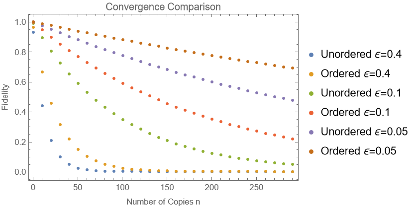
(a) Fidelity under local unitaries as $n$ grows for various choices of $q=p+\varepsilon$.

(b) Fidelity under local unitaries as $n$ grows for various choices of $q=p+\varepsilon$ compared to $F(P,Q)^{\otimes n}$.

Figure 4: Degradation of fidelity of trying to convert $n$ copies of one pure two-qubit entangle state to another for various differences in Schmidt coefficients, $q=p+\varepsilon$ where we choose $p=0.55$. (a) Shows the rate that the local unitary strategy degrades is a nonlinear function of the size of $\varepsilon$. (b) Compares to the case where one does not re-order the Schmidt coefficients, i.e. compares to $F(P,Q)^{n}$.

It is then natural to ask if what we have seen so far is something special to local unitaries. We show that under sufficient conditions, just like in the single copy case, when two-qubit seed states are involved, local unitary strategies are optimal.

Theorem 12.

Let $\ket{\psi}\in\mathbb{C}^{2}\otimes\mathbb{C}^{2}$ and the target state be $\ket{\psi}^{\otimes n}$. Let the seed state $\ket{\phi}$ satisfy $\mathrm{SR}(\ket{\phi})\leq n\mathrm{SR}(\ket{\psi})$. Then the optimal local operations strategy is the optimal local unitary strategy.

Proof.

By Theorem 6,

$$F_{LO}(\ket{\psi}^{\otimes n},\ket{\phi})$$

$$= \max_{P^{\prime}\in\mathcal{P}(\Sigma)}F((P^{\otimes n}\otimes P^{\prime})^{\downarrow},Q^{\downarrow})$$

$$= \sum_{i\in|Q|}\sqrt{Q^{\downarrow}(i)}\sqrt{(P^{\otimes n}\otimes P^{\prime})^{\downarrow}(i)}\ .$$

We will show that $P^{\prime}$ should be the delta distribution. If $p\neq 1/2$, $p^{\prime}(1)<1$, then for any $0\leq k\leq n$, we have the inequalities

$$p^{n-k}(1-p)^{k}> p^{n-k}(1-p)^{k}p^{\prime}(1)$$

$$> p^{n-k}(1-p)^{k}p^{\prime}(2)$$

and

$$p^{n-k}(1-p)^{k}> p^{n-k}(1-p)^{k}p^{\prime}(1)$$

$$> p^{n-(k+1)}(1-p)^{k+1}p^{\prime}(1)$$

$$> p^{n-(k+1)}(1-p)^{k+1}p^{\prime}(2)$$

As square root is a monotone, this holds when we take the square root. Note that by assumption $P^{\otimes n}$ has enough entries by itself for there to be one corresponding to each $q^{\downarrow}$. Therefore, given the inequalities above, it follows if $p^{\prime}(1)\neq 1$, each term in the sum only decreases. Therefore, $p^{\prime}(1)$ is optimal for every $n$ and $k$. Thus, when $p\neq 1/2$, the optimal value is obtain by $P^{\prime}$ being a delta distribution, which means it’s equivalent to the local unitary strategy.

Finally, if $p=1/2$, then $p^{n-k}(1-p)^{k}=2^{-n}$ for all $k$. Therefore, if $p^{\prime}(1)<1$, the inequalities simplifies for all $0\leq k\leq n$:

$$p^{n-k}(1-p)^{k}p^{\prime}(1)= p^{n-(k+1)}(1-p)^{k+1}p^{\prime}(1)$$

$$> p^{n-(k+1)}(1-p)^{k+1}p^{\prime}(2)$$

and

$$p^{n-k}(1-p)^{k}p^{\prime}(1)>p^{n-k}(1-p)^{k}p^{\prime}(2)\ .$$

Again because each $q$ term is paired up already, this means if $p^{\prime}(1)\neq 1$, the value decreases. Therefore, we again conclude the optimal strategy is the LU strategy. This completes the proof. ∎

We note that a trivial example of why we need the Schmidt rank constraint in the previous theorem is our original example for the advantage of LO strategies: if $\ket{\phi}^{\otimes n+\ell}$ where $\ell\geq 1$, then there is a better LO strategy than an LU strategy. Finally, we note it immediately follows from these previous results that

Corollary 4.

If $\ket{\phi},\ket{\psi}\in\mathbb{C}^{2}\otimes\mathbb{C}^{2}$ are both entangled, then

$$\lim_{n\to\infty}F_{LO}(\ket{\psi}^{\otimes n},\ket{\phi}^{\otimes n})=0\ .$$

VI On Catalytic Conversion

We now have established a rather robust theory of pure state transformations under local operations. It is natural to return to the topic of conversion of one state to another using an ancillary entanglement, i.e. cataltyic transformations, which is a special case of the setting, and includes quantum embezzlement. Of course, it is immediate from our results so far that we know the optimization program that determines the optimal pure state catalyst, as we state in the following proposition.

Proposition 15.

For any Schmidt rank $d$, the optimal pure state catalyst for state conversion $\ket{\phi}$ to $\ket{\psi}$ is the quantum state $\ket{\zeta}=\operatorname{vec}(\sqrt{R})$ that is determined via the optimization

$$\max_{R\in\mathcal{P}(d),\mathrm{P^{\prime}}\in\mathcal{P}(\Sigma)}F((P\otimes P^{\prime})^{\downarrow},(Q\otimes R)^{\downarrow})\ .$$

Proof.

This immediately follows from the input being $\ket{\phi}\otimes\operatorname{vec}(\sqrt{R})$ and then applying Theorem 6. Note this means $|\Sigma|$ scales as function of $d$. ∎

However, as we have already addressed, even without a free variable for the catalyst, the optimization in Theorem 6 seems unmanageable directly. While in principle one could use the relaxation in Theorem 9 to obtain efficient upper bounds, it is less obvious how often these will be non-trivial given that $R$ is a free variable.

The next most natural setting would be that of catalytic state conversion under local unitaries, i.e. we consider transformations of the form

$$\ket{\phi}\ket{\zeta}\xleftrightarrow{LU}\,\approx_{\varepsilon}\ket{\psi}\ket{\zeta}\ ,$$

where $\ket{\zeta}$ is the catalytic resource and the arrow going in both directions is because local unitaries are reversible. This may be seen as a generalization of embezzlement where $\ket{\phi}=\ket{0}_{A}\ket{0}_{B}$ and $\ket{\zeta}=\ket{\mu(n)}$.

Now as noted in the background, embezzling is known to be in effect optimal for sufficiently small $\varepsilon$. It follows for sufficiently small error $\varepsilon>0$, the strategy that embezzles out the seed state and then embezzles in the target state is roughly optimal, i.e.

$$\ket{\phi}\ket{\mu(n)}\xleftrightarrow{LU}\ket{0}\ket{0}\ket{\mu(n)}\xleftrightarrow{LU}\ket{\psi}\ket{\mu(n)}$$

is effectively optimal. Nonetheless, we may explore at what point this becomes necessary.

Using Theorem 5, we know the optimal strategy is given by

$$\max_{R\in\mathcal{P}(d)}F((P\otimes R)^{\downarrow},(Q\otimes R)^{\downarrow})\ .$$

Even in the case $P,Q,R\in\mathcal{P}(2)$ this technically can’t be solved using gradient methods as one has to sort the $p(1-r)$ and $(1-p)r$ terms of $p\otimes r$ and likewise for $q\otimes r$. Nonetheless, it is hopefully clear that $r\in[\min\{p,q\},\max\{p,q\}]$, as it is trying to make the distributions be more similar. Nonetheless, this issue will only grow in difficulty with the dimension and it is unclear how one would prove an ansatz is optimal in general. Therefore, we provide two-qubit examples which characterizes the general insights.

Example 4 (Resource Gap Between Embezzling and Optimal Catalyst).

Consider Bernoulli distributions $P,Q,R$ parameterized by $p=0.5,q=0.7$ and we leave $r$ unspecified for now. In other words, one of the states is the maximally entangled states and the other is, up to local unitaries, $\sqrt{0.7}\ket{00}+\sqrt{0.3}\ket{11}$. Therefore, depending on which way one runs the transformation, we are considering entanglement dilution or distillation with a catalytic resource. Without the resource,

$$F_{LO}(\ket{\psi},\ket{\phi})=F(P^{\downarrow},Q^{\downarrow})\approx 0.958.$$

One can verify that the optimal choice of $r^{\star}\approx 0.6$ in this case. For this choice

$$F_{LU}(\ket{\psi}\ket{\zeta},\ket{\phi}\ket{\zeta})= F((P\otimes R^{\star})^{\downarrow},(Q\otimes R^{\star})^{\downarrow})$$

$$> 0.979\ .$$

The first problem is that $0.979$ is not an acceptably high fidelity even by contemporary standards. Nonetheless, note that to get this state via embezzling (and ignoring that embezzling out the initial state introduces error), it would require generating $\ket{\mu(n)}$ where $n>m^{1/(1-0.979)}=2\cdot 10^{14}$. That is, even to embezzle a two-qubit pure state would require generating an inconceivable amount of entanglement. For this reason, specially engineered catalysts seems a significant improvement up to any error that can be achieved.

On the other hand, one might note that if we could generate $R$ where $r=0.55$, then we may as well have just used this state to begin with as

$$F(P^{\downarrow},R^{\downarrow})= 0.98989$$

$$> F((P\otimes R^{\star})^{\downarrow},(Q\otimes R^{\star}))\ .$$

From a practical perspective we agree with this critique. Nonetheless, from a basic science perspective, if we are interested in local unitary conversions under catalysts, then the above tells us there are better choices in general than embezzlement, although embezzling has the special property of being universal and optimal for sufficiently small $\varepsilon$.

We close this consideration with two final remarks. First, if one picks two states that are more similar to begin with, then the scaling of the embezzling state will be even larger. Second, we have not presented how the fidelity for this example scales as the local dimension of $\ket{\zeta}$ grows. Both the dimension scaling and two states that are more similar are considered in Fig. 5 where the near-optimal fidelities are found via brute force numerical search.

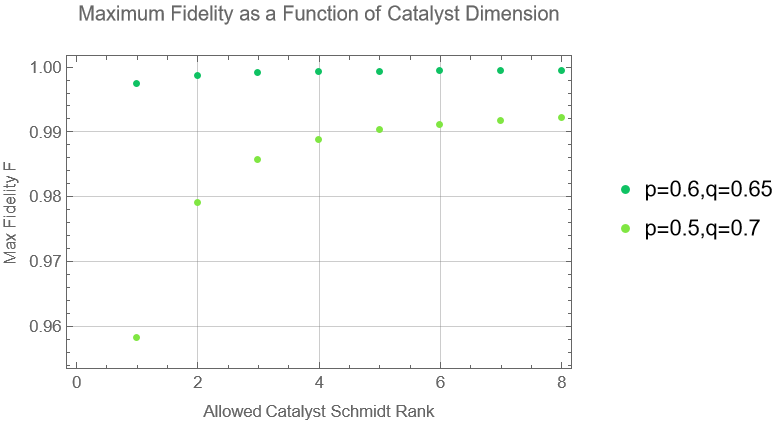
(a) Maximum achievable fidelity of transformation under local unitaries as a function of the Schmidt rank of the catalyst.

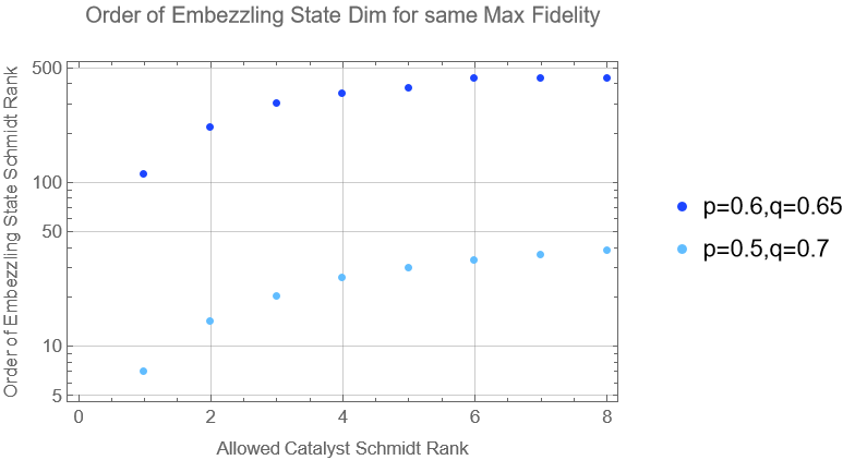
(b) Order of the Schmidt Rank of embezzling state $\ket{\mu(n)}$ to achieve same fidelity.

Figure 5: Plots regarding dimension scaling in Example 4. (a) The achievable fidelity of converting one two-qubit entangled state to another parameterized by $p$ and $q$ under local unitaries using a catalyst with a given local dimension (equivalently, Schmidt rank) using brute force search. (b) The order (i.e. the power of 10) in the Schmidt rank of the embezzling state $\ket{\mu(n)}$ to obtain the same maximum fidelity. This is calculated using $2^{1/(1-F_{\max})}$ following Proposition 3. All optimizer catalysts provided in an appendix for verification.

VII On Extensions of the Theory

As a final consideration, we discuss the application of our results beyond bipartite pure states. First we remark upon extensions to multipartite pure states. In this case the problem is that in establishing all of the results, we have used that local unitaries can take the Schmidt decomposition of the state to one of a canonical form. However, in the multipartite case, the Schmidt decomposition does not even exist in general [25]. As such this argument immediately breaks down. Furthermore, in the proof of Theorem 5 we used Uhlmann’s theorem, which requires partitioning the state into two pieces, one of which is the purification. Therefore, it seems no multipartite extension of this work holds.

Similarly, there are issues with approaching mixed states. One issue is to note that all relationships we have been able to establish have stemmed from the fidelity under local unitaries of pure states. Even in the case where local operations made a pure state no longer pure, we purified operations so that the states were pure. We simply cannot do this if we start with mixed states in both arguments of the fidelity. We also cannot purify the states as by data-processing, any optimization without tracing off the purifying space only gets us a lower bound. Moreover, this lower bound would require establishing results for tripartite systems, which returns to the issues with the multipartite pure state case. Therefore, we believe in effect these are the most general settings where these proof methods will be of use.

Appendix A Randomness Embezzling Proof and Discussion on Locality

In this section we provide the proof of Theorem 2 and then briefly discuss how it differs from quantum embezzlement.

Proof.

The proof is largely the same as for embezzlement of quantum states [12]. Let $P=\sum_{i}p(i)\outerproduct{i}{i}$. Define $W_{n}$ as $R_{n}\otimes P$ except with probabilities in decreasing order. Note

$$R_{n}\otimes P=\frac{1}{H_{n}}\sum_{i,j}\frac{p(i)}{j}\outerproduct{i}{i}\otimes\outerproduct{j}{j}\ ,$$

so there exists a relabeling on $\{(i,j)\}$ that will take this to $W_{n}$. In particular, letting $f:[m]\times[n]\to[m\cdot n]$ be a bijection, we have $\ket{i}\ket{j}\to\ket{f(i,j)}\equiv\ket{i^{\prime}}\ket{j^{\prime}}$ such that $\left\{z_{f(i,j)}:=\frac{p(i)}{jH_{n}}\right\}_{(i,j)}$ satisfy $z_{k}\geq z_{k+1}$ for all $k\in[m\cdot n]$. Therefore it suffices to approximate $W_{n}$, which means we want to bound the overlap of this with $R_{n}\otimes P$.

For fixed $t$ and $i$, we let

$$N^{t}_{i}:=\left|\left\{(i,j):\frac{p(i)}{jH_{n}}>\frac{1}{tH_{n}}\right\}\right|\ .$$

The inequality may be manipulated to imply $1\leq j<p(i)t$. It follows that $N^{t}_{i}<p(i)t$. From this we obtain $\sum_{i=1}^{m}N^{t}_{i}<\sum_{i=1}^{m}p(i)t<t$, where we have used $\sum_{i}p(i)=1$. As $z_{1}\geq z_{2}\geq...$, it follows $z_{j}\leq\frac{1}{jH_{n}}$ for all $1\geq j\geq n$. We may restate this as for $1\leq j\leq n$, there are at most $t^{\prime}-1$ pairs $(i,j)$ such that $p(i)/(jH_{n})>1/(t^{\prime}H_{n})$. Recalling $z_{1}\geq z_{2}\geq...$, this means that $z_{1}<1/H_{n}$ and that there is at most one pair $(i,j)$ pair such that $p(i)/(jH_{n})<1/(2H_{n})$, which, since $z_{1}\geq z_{2}$, means if such a pair exists, it is $z_{1}$. By applying this argument in effect recursively, we see that for $t^{\prime}$, there are at most $t^{\prime}-1$ $(i,j)$ pairs such that $p(i)/(jH_{n})>1/(t^{\prime}H_{n})$ and since $z_{k}\geq z_{k+1}$, if all of these pairs exist, then it must be $z_{1},...,z_{t^{\prime}-1}$. Therefore, $z_{j}\leq 1/(jH_{n})$ for all $1\leq j\leq n$. We can now use this to bound the fidelity.

$$F(R_{n}\otimes\outerproduct{0}{0},W_{n})= \left(\sum_{j=1}^{n}\sqrt{\frac{z_{j}}{jH_{n}}}\right)^{2}$$

$$\geq \left(\sum_{j=1}^{n}\sqrt{z_{j}}\right)^{2}\geq\sum_{j=1}^{n}z_{j},$$

where in the equality we have used the definition of fidelity, in the second we used our established inequality, and in the third we have used $\sqrt{x}+\sqrt{y}\geq\sqrt{x+y}$ for $x,y\geq 0$ to pull the square root out around the sum and cancel with the square.

Now we want to lower bound this sum, which requires managing the $z_{j}$ terms. We consider $T_{n}=R_{n}\otimes\pi_{m}$ with probabilities $t(j)$ where $\pi_{m}:=\frac{1}{m}\sum_{i=1}^{m}\outerproduct{i}{i}$. Now note that $z_{k}\geq t_{k}$ for all $k\in[m\cdot n]$, and this is independent of what the distribution $P$ is. We can then bound the relevant sum by the sum for $T_{n}$. It follows

$$\sum_{j=1}^{n}t_{j}=\sum_{j=1}^{\lfloor n/m\rfloor}\sum_{i=1}^{m}\frac{1}{jH_{n}m}= \sum_{j=1}^{\lfloor n/m\rfloor}\frac{1}{jH_{n}}$$

$$= \frac{H_{\lfloor n/m\rfloor}}{H_{m}}$$

$$\geq \frac{\ln(n/m)}{\ln(n)}=1-\frac{\log(m)}{\log(n)}\ ,$$

where the second inequality is using $H_{n}\geq\ln(n)$ and the final form is converting from $\ln$ to $\log$ in both the numerator and denominator so it cancels. Finally, leting $1-\log(m)/\log(n)>1-\varepsilon$ will result in $n>m^{1/\varepsilon}$, which completes the proof. ∎

With the proof established, we expand upon the distinction between the entangled and classical distribution cases of embezzlement in terms of locality briefly mentioned in the main text. In the classical case, one party embezzles a distribution locally by themselves, whereas in the entangled case two parties act locally on a non-local distribution. Mathematically, this simply follows from the fact the $\operatorname{vec}(\cdot)$ map and its inverse converts between bipartite states and a probability distribution. However, it is also physically interesting that these are the two cases that align as it is clear other variations are either classically or quantumly impossible as we now explain.

The first reasonable variation would be if there is a non-local classical case where two parties try and construct some joint distribution $p_{XY}$ using catalyst $r_{X^{\prime}Y^{\prime}}$. It is easy to see that they cannot in general satisfy the decoupling condition that is satisfied in quantum embezzlement, i.e. they cannot satisfy $p_{XY}\otimes r_{X^{\prime}Y^{\prime}}$ in this setting. This is because without loss of generality the state will be of the form

$$q_{XYX^{\prime}Y^{\prime}}= \sum_{x,x^{\prime},y,y^{\prime}}q(x|x^{\prime})q^{\prime}(y|y^{\prime})r(x,y)$$

$$\hskip 56.9055pt\cdot\outerproduct{x,y,x^{\prime},y^{\prime}}{x,y,x^{\prime},y^{\prime}}\ .$$

This form means that $X$ will be correlated to $X^{\prime}$ and $Y$ to $Y^{\prime}$ unless $q_{XY}$ may be generated non-locally without a seed state to correlate the two which means they are (up to the allowed error) independent, i.e. $q_{XY}\approx_{\varepsilon}q_{X}\otimes q_{Y}$. In this sense, there cannot be a classical non-local equivalent of quantum embezzlement.

On the other hand, if one does not require the decoupling, then this is a task that is possible in the classical setting and is known as distributed source simulation, where the question is the minimal needed shared randomness as the seed state to generate the target state up to an (arbitrary) error [26]. This was determined asymptotically in the classical case by Wyner [8], extended to separable states by Hayashi [9], and recently generalized to the one-shot setting for separable states in [10]. However, as in this setting variation there is no communication between the acting parties and the catalyst acts as the seed state, it follows from Proposition 2 that distributed source simulation cannot admit an entangled state equivalent. For these reasons, not only does the $\operatorname{vec}$ bijection specify the correspondence of embezzlement in the classical and quantum setting, but deviating from it makes either a quantum or classical version impossible.

Appendix B Semidefinite Program Relaxation of Max Fidelity of Pure State Transformation Under LOSR

In this section we prove Theorem 9. We begin by establishing (7) is true.

Lemma 13.

Consider target state $\ket{\psi}$ and seed state $\ket{\phi}$. Let $\mathrm{SR}(\psi)=d$ and $\mathrm{SR}(\phi)=d^{\prime}$. Define $A=\mathbb{C}^{d}$, $B=\mathbb{C}^{d\cdot d^{\prime}}$. Then,

$$F_{\mathrm{LOSR}}(\ket{\psi},\ket{\phi})\leq\max \;F(R,Q^{\downarrow}_{\text{embed}})$$

$$\mathrm{s.t.} \;\Tr_{B}[R]=P^{\downarrow}$$

$$\;R\in\mathcal{P}^{\downarrow}(d^{2}\cdot d^{\prime})\ ,$$

where $P$ and $Q$ are the distributions defined by $\ket{\psi}$ and $\ket{\phi}$’s Schmidt coefficients respectively.

Proof.

The above seems intuitively true from Theorem 6 as we have just relaxed the tensor product structure with the partial trace constraint. The technical issue is the ordering operation $\cdot^{\downarrow}$ is defined in terms of a permutation of a fixed basis, so we need to make sure this works with the partial trace.

Note the feasible set, the set we can optimizer over, in Theorem 6 is $S_{1}(P):=\{(P\otimes P^{\prime})^{\downarrow}:P^{\prime}\in\mathcal{P}(\Sigma)\}$. Now note this is the same as the set

$$S_{2}(P):=\{(P^{\downarrow}\otimes{P^{\prime}}^{\downarrow})^{\downarrow}:P^{\prime}\in\mathcal{P}(\Sigma)\}\ ,$$

because the ordering applied to the tensor product will result in the same thing regardless of whether or not $P,P^{\prime}$ were ordered. Therefore, we can focus on $P^{\downarrow}\otimes{P^{\prime}}^{\downarrow}$ to make the explanation clearer.

In general, in terms of vectors,

$$(p^{\downarrow}\otimes{p^{\prime}}^{\downarrow})^{\downarrow}=\begin{pmatrix}p^{\downarrow}(1){p^{\prime}}^{\downarrow}\\ p^{\downarrow}(2){p^{\prime}}^{\downarrow}\\ \vdots\\ p^{\downarrow}(d){p^{\prime}}^{\downarrow}\end{pmatrix}\ ,$$

where $p(i)\geq p(i+k)$ for $k\geq 0$. Formally, we also have

$$p^{\downarrow}(i){p^{\prime}}^{\downarrow}(1)\geq p^{\downarrow}(i+k){p^{\prime}}^{\downarrow}(j)$$

for all $i\in[d]$, $k\in\{0,...,d-i\}$, and $j\in\Sigma$. In particular what this means is that without loss of generality for any $i\in[d]$, $p^{\downarrow}(i){p^{\prime}}^{\downarrow}(1)$ appears before any element that is not of the form $p^{\downarrow}(i-\ell){p^{\prime}}^{\downarrow}(j)$ for some $0<\ell\leq i-1$. It follows that under the ordering of $(p^{\downarrow}\otimes{p^{\prime}}^{\downarrow})^{\downarrow}$, when the partial trace marginalizes to the $A$ space, the induced ordering on the local space will be the ordering based on $p^{\downarrow}$. Formally, this can be expressed as

$$\Tr_{\mathbb{C}^{|\Sigma|}}[(P^{\downarrow}\otimes{P^{\prime}}^{\downarrow})^{\downarrow}]$$

$$= \sum_{j\in\Sigma}\mathbb{1}_{A}\otimes\bra{j}(P^{\downarrow}\otimes{P^{\prime}}^{\downarrow})^{\downarrow}\ket{j}$$

$$= \sum_{i\in[d]}p^{\downarrow}(i)\outerproduct{i}{i}\ ,$$

where the first equality is a representation of the partial trace and the second is using the property noted of the ordering on the joint ordered distribution.

Thus, if $X\in S_{2}(P)$, $\Tr_{C^{|\Sigma|}}(X)=P^{\downarrow}$ and $X\in\mathcal{P}^{\downarrow}(d\cdot|\Sigma|)$. Noting that $|\Sigma|=d\cdot d^{\prime}$, this is the feasible set we have defined in the proposition. This completes the proof. ∎

The remaining point is to prove this is the semidefinite program given in (8). There is much to the theory of semidefinite programs for quantum information [19], but for our purposes all we will need is the following definition.

Definition 2.

A semidefinite program may be expressed as

$$\max \Tr(AX)$$

s.t. $$\;\Phi(X)=B$$

$$X_{\mathbb{C}^{d}}\preceq 0\ ,$$

where $\Phi\in\mathrm{T}(\mathbb{C}^{d},\mathbb{C}^{d^{\prime}})$ is a Hermitian-preserving map, $A\in\mathrm{Herm}(\mathbb{C}^{d})$, $B\in\mathrm{Herm}(\mathbb{C}^{d^{\prime}})$, and $\mathrm{Herm}(\cdot)$ is the space of Hermitian operators on a given Hilbert space.

The fidelity is known to be a semidefinite program [19], so we are really just verifying all of our constraints work and that we can write the SDP simply by making use of that.

Lemma 14.

The optimization program in the previous lemma, may be expressed as the following semidefinite program over the reals.

$$\max \sum_{i\in[d^{2}\cdot d^{\prime}]}x(i)$$

s.t. $$\;\begin{pmatrix}\text{diag}(r)&\text{diag}(x)\\ \text{diag}(x)&\text{diag}(q^{\downarrow}_{\text{embed}})\end{pmatrix}\succeq 0$$

$$\Tr_{B}[\text{diag}(r)]=P^{\downarrow}$$

$$r\in\mathcal{P}^{\downarrow}([d^{2}\cdot d])$$

$$x\in\mathbb{R}^{d^{2}\cdot d^{\prime}}\ ,$$

where $d,d^{\prime}$ are defined in the previous lemma.

Proof.

We begin by expressing the objective function of the previous lemma, which is in terms of fidelity, using the primal problem for the SDP for fidelity from [19, Theorem 3.17]:

$$\max \frac{1}{2}\left[\Tr(X)+\Tr(X^{\dagger})\right]$$

$$\;\begin{pmatrix}R&X\\ X^{\dagger}&Q^{\downarrow}_{\text{embed}}\end{pmatrix}\geq 0$$

$$X\in\mathrm{L}(\mathbb{C}^{[d^{2}\cdot d^{\prime}]})\ .$$

Now our goal is to reduce $X$ to the diagonal of a real vector.

Note that $R,Q^{\downarrow}_{\text{embed}}$ are always invariant under pinching onto the computational basis of $\mathbb{C}^{[d^{2}\cdot d^{\prime}]}$, which we can denote $\Delta$. Note that this pinching is a CPTP, so by the CP property,

$$(\mathrm{id}_{\mathbb{C}^{2}}\otimes\Delta)\begin{pmatrix}R&X\\ X^{\dagger}&Q^{\downarrow}_{\text{embed}}\end{pmatrix}$$

$$= \begin{pmatrix}R&\Delta(X)\\ \Delta(X^{\dagger})&Q^{\downarrow}_{\text{embed}}\end{pmatrix}\geq 0\ .$$

It also then follows as a positive semidefinite operator is always Hermitian that

$$\begin{pmatrix}R&\Delta(X^{\dagger})\\ \Delta(X)&Q^{\downarrow}_{\text{embed}}\end{pmatrix}\geq 0\ .$$

Thus by taking these two cases and averaging them, we have that

$$\begin{pmatrix}R&\frac{1}{2}\left(\Delta(X+X^{\dagger})\right)\\ \frac{1}{2}\left(\Delta(X+X^{\dagger})\right)&Q^{\downarrow}_{\text{embed}}\end{pmatrix}\geq 0\ .$$

Define $\overline{X}:=\frac{1}{2}\left(\Delta(X+X^{\dagger})\right)$. Then note

$$\frac{1}{2}\left(\Tr(X)+\Tr(X^{\dagger})\right)$$

$$= \frac{1}{2}\left(\Tr(\Delta(X))+\Tr(\Delta(X^{\dagger}))\right)$$

$$= \frac{1}{2}\left(\Tr(\overline{X})+\Tr(\overline{X}^{\dagger})\right)=\Tr(\overline{X})\ ,$$

where the first equality is because the pinching is trace preserving, the second is by definition of $\overline{X}$, as is the final equality. Thus, for any $X$ that satisfies the positivity constraint, we could replace it with $\overline{X}$ without loss of generality as we are considering a maximization. Finally, note that $\overline{X}$ is a real diagonal matrix by the pinching along with the fact $a+a^{\ast}=2\Re{a}$. Thus $\overline{X}=\text{diag}(x)$ for some $x\in\mathbb{R}^{d^{2}\cdot d^{\prime}}$. Combining all these points and using $\Tr(\overline{X})=\sum_{i\in[d^{2}\cdot d^{\prime}]}x(i)$, we have reduced to considering

$$\max \sum_{i\in[d^{2}\cdot d^{\prime}]}x(i)$$

$$\;\begin{pmatrix}\text{diag}(r)&\text{diag}(x)\\ \text{diag}(x)&\text{diag}(q^{\downarrow}_{\text{embed}})\end{pmatrix}\geq 0$$

$$x\in\mathbb{R}^{d^{2}\cdot d^{\prime}}\ .$$

This argument works for any choice of diagonal $r$, so this is the major reduction.

What remains is to prove all the constraints are Hermitian maps. One can write the constraints for $r\in\mathcal{P}^{\downarrow}$ as $r(i)\geq r(i+1)$ for all $i$, which are semidefinite constraints and can be written as Hermitian preserving maps on the variables $r,x$. diag is a Hermitian preserving map as is the partial trace, so $\Tr_{C}[\text{diag}(r)]$ is a Hermitian preserving map. Likewise is the block matrix mapping if one allows for the complex conjugate in the lower left block, but noting $\text{diag}(x)^{\dagger}=\text{diag}(x)$, we can leave it as written. Thus all the maps are Hermitian-preserving.

The conversion to actual standard form we then omit as it provides no insight. This completes the proof. ∎

The above two proofs establish Theorem 9.

Appendix C Data for Catalyst Figure

For $p=0.5,q=0.7$:

Dimension	Optimal distribution $r$
1	n/a
2	$\frac{1}{100}[4,6]$
3	$\frac{1}{100}[21,32,47]$
4	$\frac{1}{100}[12,18.5,0.28,0.415]$
5	$\frac{1}{100}[7,11,17,26,39]$
6	$\frac{1}{100}[5,8,11,16,24,35]$
7	$\frac{1}{100}[3,5,8,11,16,23,24]$
8	$\frac{1}{100}[5,6,9,9,13,14,19,25]$

For $p=0.6,q=0.65$:

Dimension	Optimal distribution $r$
1	n/a
2	$\frac{1}{100}[32,63]$
3	$\frac{1}{100}[18,31,51]$
4	$\frac{1}{100}[10,17,28,45]$
5	$\frac{1}{100}[6,10,16,26,42]$
6	$\frac{1}{100}[7,11,12,18,20,32]$
7	$\frac{1}{100}[0,7,11,12,18,20,32]$
8	$\frac{1}{100}[0,0,7,11,12,18,20,32]$

References

- Wheeler [1989] J. A. Wheeler, Information, physics, quantum: The search for links, in Proceedings III International Symposium on Foundations of Quantum Mechanics (1989) pp. 354–358.
- Zur [1990] Complexity, Entropy, and the Physics of Information, Vol. VIII (Addison-Wesley, The Advanced Book Program, 1990).
- Landauer [1991] R. Landauer, Information is physical, Physics Today 44, 23 (1991).
- Chitambar and Gour [2019] E. Chitambar and G. Gour, Quantum resource theories, Reviews of Modern Physics 91, 025001 (2019).
- Bell [1964] J. S. Bell, On the einstein podolsky rosen paradox, Physics Physique Fizika 1, 195 (1964).
- Hayden and Winter [2003] P. Hayden and A. Winter, Communication cost of entanglement transformations, Physical Review A 67, 012326 (2003).
- Harrow and Lo [2004] A. Harrow and H.-K. Lo, A tight lower bound on the classical communication cost of entanglement dilution, IEEE Transactions on Information Theory 50, 319 (2004).
- Wyner [1975] A. Wyner, The common information of two dependent random variables, IEEE Transactions on Information Theory 21, 163 (1975).
- Hayashi [2006] M. Hayashi, Quantum Information: An Introduction (Springer, 2006).
- George et al. [2022] I. George, M.-H. Hsieh, and E. Chitambar, One-shot distributed source simulation: As quantum as it can get (2022), in Preparation.
- Schmid et al. [2021] D. Schmid, H. Du, M. Mudassar, G. Coulter-de Wit, D. Rosset, and M. J. Hoban, Postquantum common-cause channels: the resource theory of local operations and shared entanglement, Quantum 5, 419 (2021).
- van Dam and Hayden [2003] W. van Dam and P. Hayden, Universal entanglement transformations without communication, Physical Review A 67, 060302 (2003).
- Bennett et al. [2014] C. H. Bennett, I. Devetak, A. W. Harrow, P. W. Shor, and A. Winter, The quantum reverse shannon theorem and resource tradeoffs for simulating quantum channels, IEEE Transactions on Information Theory 60, 2926 (2014).
- Anshu et al. [2021] A. Anshu, S. B. Hadiashar, R. Jain, A. Nayak, and D. Touchette, One-shot quantum state redistribution and quantum markov chains, in 2021 IEEE International Symposium on Information Theory (ISIT) (IEEE, 2021) pp. 130–135.
- Leung and Wang [2014] D. Leung and B. Wang, Characteristics of universal embezzling families, Phys. Rev. A 90, 042331 (2014).
- Dinur et al. [2015] I. Dinur, D. Steurer, and T. Vidick, A parallel repetition theorem for entangled projection games, Computational Complexity 24, 201 (2015).
- Hayden et al. [2004] P. Hayden, R. Jozsa, D. Petz, and A. Winter, Structure of states which satisfy strong subadditivity of quantum entropy with equality, Communications in mathematical physics 246, 359 (2004).
- Wilde [2011] M. M. Wilde, From classical to quantum shannon theory, arXiv preprint arXiv:1106.1445 (2011).
- Watrous [2018] J. Watrous, The Theory of Quantum Information (Cambridge University Press, 2018).
- de Vicente and Huber [2011] J. I. de Vicente and M. Huber, Multipartite entanglement detection from correlation tensors, Physical Review A 84, 062306 (2011).
- Mudholkar and Freimer [1985] G. S. Mudholkar and M. Freimer, A structure theorem for the polars of unitarily invariant norms, Proceedings of the American Mathematical Society 95, 331 (1985).
- Johnston [2012] N. Johnston, Norms and Cones in the Theory of Quantum Entanglement, Ph.D. thesis, University of Guelph (2012).
- Bennett et al. [1996] C. H. Bennett, H. J. Bernstein, S. Popescu, and B. Schumacher, Concentrating partial entanglement by local operations, Physical Review A 53, 2046 (1996).
- Cover and Thomas [2006] T. M. Cover and J. A. Thomas, Elements of Information Theory (John Wiley & Sons, Inc., 2006).
- Peres [1995] A. Peres, Higher order schmidt decompositions, arXiv preprint quant-ph/9504006 (1995).
- Yu and Tan [2022] L. Yu and V. Y. F. Tan, Common information, noise stability, and their extensions, Foundations and Trends® in Communications and Information Theory 19, 107 (2022).