Construction of Wannier functions from the spectral moments of correlated electron systems

Abstract

When the first four spectral moments are considered, spectral features missing in standard Kohn-Sham (KS) density-functional theory (DFT), such as upper and lower Hubbard bands, as well as spectral satellite peaks, can be described, and the bandwidths can be corrected. Therefore, we have devised a moment-functional based spectral density functional theory (MFbSDFT) recently. However, many computational tools in theoretical solid state physics, such as the construction of maximally localized Wannier functions (MLWFs), have been developed for KS-DFT and require modifications if they are supposed to be used in MFbSDFT. Here, we show how generalized Wannier functions may be constructed from the first four spectral moment matrices. We call these functions maximally localized spectral moment Wannier functions (MLSMWFs). We demonstrate how MLSMWFs may be used to compute the anomalous Hall effect (AHE) in fcc Ni by Wannier interpolation. More generally, MLSMWFs may be computed from the first $2P$ moments ($P=1,2,3,\dots$). Using more than 4 moments opens the perspective of reproducing all spectral features accurately in MFbSDFT.

I Introduction

Maximally localized Wannier functions (MLWFs) have become a widely-applied tool in computational solid state physics. Recent reviews [1, 2] give a comprehensive overview of their applications. Using Wannier interpolation [3] one may significantly reduce the computing time requirements of calculations of response functions such as the anomalous Hall effect (AHE) [4], thermoelectric coefficients [5], and the spin-orbit torque (SOT) [6, 7].

The Wannier interpolation of the AHE does not suffer from band truncation errors, because it directly interpolates the Berry curvature. In order to interpolate the SOT and the Dzyaloshinskii-Moriya interaction without band truncation errors one may use higher-dimensional Wannier functions [8] in order to interpolate the mixed Berry curvature [9, 10]. Response functions that cannot be expressed in terms of these geometric properties of the electronic bands cannot be treated within the conventional Wannier interpolation method without any band truncation error. However, for such response functions Wannier function perturbation theory has been developed recently [11].

All these MLWF-based interpolation methods have been devised essentially in the context of KS-DFT. While impressive progress has been achieved in developing exchange-correlation functionals for KS-DFT that describe ground state properties of solids with high precision [12], experimental spectra are often not reproduced well by standard KS-DFT [13]. In Ref. [14] and in Ref. [15] we have explained how the spectral function may be constructed from the first four spectral moment matrices. These moment matrices may be obtained either by computing several correlation functions self-consistently [14], or by evaluating suitable moment functionals [15]. We expect that the moment potentials required for the latter approach, which we call MFbSDFT, are universal functionals of the spin density.

Indeed, we have shown that parameter-free moment functionals can be found that improve the spectra of Na and SrVO₃ significantly [16] in comparison to standard KS-DFT with LDA. In order to formulate these parameter-free moment functionals we have used an existing model of the second moment of the uniform electron gas (UEG) [17] as well as models of the momentum distribution function $n_{{\bm{k}}}$ of the UEG [18, 19, 20]. However, formulating universal moment functionals that are generally applicable is still a long way. Notably, the correct inclusion of spin-polarization and the extension by gradient corrections are important necessary developments left for future work.

Nevertheless, even while the universal moment functionals are not yet available, one may generally improve spectra by optimizing the parameters in suitable parameterized moment functionals. Adjusting in this way e.g. the bandwidths and gaps in order to reproduce experimental data will increase the accuracy of response function calculations, in particular those of optical responses, such as laser-induced currents [21] and torques [22], which are expected to be generally sensitive to gaps, bandwidths, and band positions, because they are not Fermi-surface effects like the AHE [23, 24, 25] for example.

We have demonstrated that MFbSDFT can be used to improve the description of the electronic structure of fcc Ni significantly in comparison to LDA, because it yields bandwidth, exchange splitting, and satellite peak positions in good agreement with the experimental spectrum [15, 16]. The satellite peak in Ni roughly 6 eV below the Fermi energy is a correlation effect [26, 27, 28], which is missing in the KS-spectrum. Since the method of spectral moments captures the splitting of bands into lower and upper Hubbard bands, it cannot be mapped onto a non-interacting effective KS Hamiltonian in general without changing the spectrum. The question therefore poses itself of how to obtain generalized Wannier functions from the spectral moment matrices.

The method of spectral moments yields state energies, state wavefunctions, and corresponding spectral weights, in contrast to KS-DFT, where the spectral weights are by definition unity. Moreover, the state wavefunctions corresponding to different energies are not guaranteed to be orthogonal. While many-body generalizations of Wannier functions have been considered before [29], these generalizations are not optimized to construct localized Wannier functions from the first four spectral moment matrices. For example, Ref. [29] does not take the spectral weights of the quasiparticles into account and does not consider the possibility that the quasiparticle wavefunctions do not necessarily form a set of mutually orthogonal functions. However, the standard method of constructing MLWFs assumes the Bloch functions of different bands to be orthogonal [30, 31]. Here, we will show that spectral weights and non-orthogonality of quasiparticle wavefunctions can be taken into account by generalizing the MLWFs concept for the method of spectral moments.

We demonstrate the construction of MLSMWFs for fcc Ni and use them to compute the AHE by Wannier interpolation. We choose fcc Ni because it is known that standard KS-DFT overestimates the bandwidth and the exchange splitting in this material [27] and it predicts the AHE to be significantly larger than the experimental value [32, 33, 34]. Moreover, even the sign of the magnetic anisotropy energy (MAE) is not predicted correctly by standard KS-DFT, i.e., LDA does not predict the correct easy axis [35]. Previously, we have demonstrated that MFbSDFT can be used to reproduce the experimental values of the exchange splitting, the bandwidth, and the position of the satellite peaks [15, 16]. Here, we demonstrate that also the AHE is predicted to be close to the experimental value if MFbSDFT is used.

The rest of this paper is structured as follows. In Sec. II we explain how we construct MLSMWFs from the first four spectral moment matrices. Practical issues, such as the use of the wannier90 code [2] for the generation of MLSMWFs are described in Sec. II.5 and in Sec. II.6. MLSMWFs with spin-orbit interaction (SOI) are discussed in Sec. II.7. In Sec. II.8 we explain that ab-initio programs which can compute MLWFs can be extended easily to compute additionally MLSMWFs. In Sec. II.9 we describe Wannier interpolation based on MLSMWFs using the example of the AHE. The interpolation of additional matrix elements such as spin and torque operators is discussed in Sec. II.10. In Sec. III we explain how the method of Sec. II may be generalized to include the first $2P$ moments ($P=3,4,\dots$). In Sec. IV we present applications of our method to fcc Ni. This paper ends with a summary in Sec. V.

II Theory

Before discussing the construction of MLSMWFs from the first four spectral moment matrices in Sec. II.4 we first revisit the generation of MLWFs in Sec. II.1 as well as the calculation of the spectral function in Sec. II.2. This will help us to explain the necessary modifications of the MLWFs formalism in Sec. II.4, when MLSMWFs are constructed from the spectral moment matrices.

II.1 MLWFs and Wannier interpolation

The Bloch functions $|\psi_{{\bm{k}}m}\rangle$ are eigenfunctions of the KS-Hamiltonian $H$ with eigenenergies $\mathcal{E}_{{\bm{k}}m}$:

$$H|\psi_{{\bm{k}}m}\rangle=\mathcal{E}_{{\bm{k}}m}|\psi_{{\bm{k}}m}\rangle,$$ (1)

where ${\bm{k}}$ is the ${\bm{k}}$-point and $m$ is the band index. The MLWFs $|W_{{\bm{R}}n}\rangle$ are constructed from these Bloch functions by the transformation [30]

$$|W_{{\bm{R}}n}\rangle=\frac{1}{\mathcal{N}}\sum_{{\bm{k}}}\sum_{m=1}^{N_{\rm B}}U_{mn}^{({\bm{k}})}e^{-i{\bm{k}}\cdot{\bm{R}}}|\psi_{{\bm{k}}m}\rangle,$$ (2)

where $\mathcal{N}$ is the number of ${\bm{k}}$ points. The matrix ${\bm{U}}^{({\bm{k}})}$ is a rectangular matrix when the number of bands $N_{\rm B}$ is larger than the number of MLWFs $N_{\rm W}$, otherwise it is a square matrix, which may occur for example when MLWFs are constructed from isolated groups of bands [31]. The matrix ${\bm{U}}^{({\bm{k}})}$ is determined by the condition that the MLWFs minimize the spatial spread

$$\Omega=\sum_{n=1}^{N_{\rm W}}\left[\langle W_{{\bm{R}}n}|{\bm{r}}^{2}|W_{{\bm{R}}n}\rangle-\left(\langle W_{{\bm{R}}n}|{\bm{r}}|W_{{\bm{R}}n}\rangle\right)^{2}\right].$$ (3)

Due to the localization of the MLWFs in real-space the matrix elements of the Hamiltonian $H$ decay rapidly when the distance between the MLWFs increases:

$$\lim_{{\bm{R}}\rightarrow\infty}\langle W_{{\bm{0}}m}|H|W_{{\bm{R}}n}\rangle\rightarrow 0.$$ (4)

This localization property is important for Wannier interpolation, because it implies that in order to interpolate the electronic structure at any desired ${\bm{k}}$ point it is sufficient to provide the matrix elements $\langle W_{{\bm{0}}m}|H|W_{{\bm{R}}n}\rangle$ for a finite and small set of ${\bm{R}}$ vectors. The reason for this is that the electronic structure at any desired ${\bm{k}}$ point may be computed by performing a Fourier transformation of $\langle W_{{\bm{0}}m}|H|W_{{\bm{R}}n}\rangle$ and that the computational time for this is small if the set of ${\bm{R}}$ vectors is small. Explicitly, the matrix elements of the Hamiltonian may be written as

$$\langle W_{{\bm{0}}m}|H|W_{{\bm{R}}n}\rangle=$$ (5)

$$=\frac{1}{\mathcal{N}}\sum_{{\bm{k}}}\sum_{m^{\prime}=1}^{N_{\rm B}}e^{-i{\bm{k}}\cdot{\bm{R}}}\mathcal{E}_{{\bm{k}}m^{\prime}}\left[U^{({\bm{k}})}_{m^{\prime}m}\right]^{*}U^{({\bm{k}})}_{m^{\prime}n}.$$

In order to describe the AHE in magnetically collinear ferromagnets, the spin-orbit interaction (SOI) has to be taken into account. Wannier interpolation is very efficient in computing the AHE [4]. In the presence of SOI, the Bloch functions are spinors

$$\langle{\bm{r}}|\psi_{{\bm{k}}m}\rangle=\psi_{{\bm{k}}m}({\bm{r}})=\begin{pmatrix}\chi_{{\bm{k}}m\uparrow}({\bm{r}})\\ \chi_{{\bm{k}}m\downarrow}({\bm{r}})\end{pmatrix},$$ (6)

and the MLWFs are spinors as well:

$$\langle{\bm{r}}|W_{{\bm{R}}n}\rangle=\begin{pmatrix}W_{{\bm{R}}n\uparrow}({\bm{r}})\\ W_{{\bm{R}}n\downarrow}({\bm{r}})\end{pmatrix}.$$ (7)

For the interpolation of the AHE in bcc Fe [4] one first constructs MLWFs using a coarse ${\bm{k}}$ mesh, e.g. an $8\times 8\times 8$ mesh. Next, one computes the matrix elements of the Hamiltonian according to Eq. (5). Finally, one may Fourier transform these matrix elements for all ${\bm{k}}$ points in the fine interpolation mesh, e.g. an $800\times 800\times 800$ mesh. Using this interpolated Hamiltonian, one may compute the AHE numerically efficiently [4].

II.2 Construction of the spectral function from the first four spectral moment matrices

In Ref. [15] we describe an algorithm to construct the spectral function from the first four spectral moments. In the following we assume that the spectral moments are so expressed in a basis set of $N_{\rm S}$ orthonormalized functions $\phi_{{\bm{k}}n}({\bm{r}})$ that they are given by $N_{\rm S}\times N_{\rm S}$ matrices. Due to the orthonormalization of the basis functions, the zeroth moment ${\bm{M}}_{{\bm{k}}}^{(0)}$ is simply the unit matrix. When the spectral function is determined approximately from the first four spectral moments (${\bm{M}}_{{\bm{k}}}^{(0)}$, ${\bm{M}}_{{\bm{k}}}^{(1)}$, ${\bm{M}}_{{\bm{k}}}^{(2)}$, and ${\bm{M}}_{{\bm{k}}}^{(3)}$), the poles of the single-particle spectral function are given by the eigenenergies of the hermitean $2N_{\rm S}\times 2N_{\rm S}$ matrix [15]

$${\bm{\mathcal{H}}}_{{\bm{k}}}=\left(\begin{array}[]{cc}{\bm{M}}_{{\bm{k}}}^{(1)}&{\bm{B}}_{1{\bm{k}}}\\ {\bm{B}}_{1{\bm{k}}}^{\dagger}&{\bm{D}}_{1{\bm{k}}}\end{array}\right),$$ (8)

where ${\bm{M}}_{{\bm{k}}}^{(1)}$ is the first moment, ${\bm{B}}_{1{\bm{k}}}={\bm{\mathcal{U}}}_{{\bm{k}}}\sqrt{{\bm{\mathcal{D}}}_{{\bm{k}}}}$, ${\bm{B}}_{2{\bm{k}}}=[{\bm{M}}_{{\bm{k}}}^{(3)}-{\bm{M}}_{{\bm{k}}}^{(2)}{\bm{M}}_{{\bm{k}}}^{(1)}][{\bm{B}}_{1{\bm{k}}}^{\dagger}]^{-1}$, and ${\bm{D}}_{1{\bm{k}}}={\bm{B}}_{1{\bm{k}}}^{-1}[{\bm{B}}_{2{\bm{k}}}-{\bm{M}}_{{\bm{k}}}^{(1)}{\bm{B}}_{1{\bm{k}}}]$. Here, ${\bm{\mathcal{D}}}_{{\bm{k}}}$ is a diagonal matrix, and ${\bm{\mathcal{U}}}_{{\bm{k}}}$ is a unitary matrix so that ${\bm{\mathcal{U}}}_{{\bm{k}}}{\bm{\mathcal{D}}}_{{\bm{k}}}{\bm{\mathcal{U}}}_{{\bm{k}}}^{\dagger}={\bm{M}}_{{\bm{k}}}^{(2)}-{\bm{M}}_{{\bm{k}}}^{(1)}{\bm{M}}_{{\bm{k}}}^{(1)}$.

The eigenvectors of ${\bm{\mathcal{H}}}_{{\bm{k}}}$, Eq. (8), may be written as

$${\bm{\Psi}}_{{\bm{k}}n}=\begin{pmatrix}{\bm{\psi}}_{{\bm{k}}n\rightarrow}\\ {\bm{\psi}}_{{\bm{k}}n\leftarrow}\end{pmatrix},$$ (9)

where ${\bm{\psi}}_{{\bm{k}}n\rightarrow}$ and ${\bm{\psi}}_{{\bm{k}}n\leftarrow}$ are both column vectors with $N_{\rm S}$ components, while ${\bm{\Psi}}_{{\bm{k}}n}$ is a column vector with $2N_{\rm S}$ entries. We denote the eigenvalues of ${\bm{\mathcal{H}}}_{{\bm{k}}}$ by $\mathscr{E}_{{\bm{k}}n}$, i.e.,

$${\bm{\mathcal{H}}}_{{\bm{k}}}{\bm{\Psi}}_{{\bm{k}}n}=\mathscr{E}_{{\bm{k}}n}{\bm{\Psi}}_{{\bm{k}}n}.$$ (10)

Within MFbSDFT, the charge density is computed only from the upper part ${\bm{\psi}}_{{\bm{k}}n\rightarrow}$ of the state vector ${\bm{\Psi}}_{{\bm{k}}n}$ (Eq. (9)), while the lower part plays the role of an auxiliary component. Note that while the eigenfunctions $|\psi_{{\bm{k}}m}\rangle$ of the KS-Hamiltonian (Eq. (1)) are orthonormal, i.e.,

$$\langle\psi_{{\bm{k}}m}|\psi_{{\bm{k}}^{\prime}n}\rangle=\delta_{nm}\delta_{{\bm{k}}{\bm{k}}^{\prime}},$$ (11)

the upper parts ${\bm{\psi}}_{{\bm{k}}n\rightarrow}$ of the state vectors ${\bm{\Psi}}_{{\bm{k}}n}$ (Eq. (9)) are not even orthogonal, i.e.,

$$\left[{\bm{\psi}}_{{\bm{k}}m\rightarrow}\right]^{\dagger}{\bm{\psi}}_{{\bm{k}}n\rightarrow}\not\propto\delta_{nm},$$ (12)

while the complete state vectors are orthonormal:

$$\left[{\bm{\Psi}}_{{\bm{k}}m}\right]^{\dagger}{\bm{\Psi}}_{{\bm{k}}n}=\delta_{nm}.$$ (13)

We may obtain the spectral weight of the state ${\bm{\Psi}}_{{\bm{k}}n}$ from

$$a_{{\bm{k}}n}=\left[{\bm{\psi}}_{{\bm{k}}n\rightarrow}\right]^{\dagger}{\bm{\psi}}_{{\bm{k}}n\rightarrow}=\sum_{m^{\prime}=1}^{N_{\rm S}}[{\bm{\psi}}_{{\bm{k}}nm^{\prime}\rightarrow}]^{*}{\bm{\psi}}_{{\bm{k}}nm^{\prime}\rightarrow}.$$ (14)

Here, $\psi_{{\bm{k}}nm^{\prime}\rightarrow}$ is the $m^{\prime}$-th entry in the column vector ${\bm{\psi}}_{{\bm{k}}n\rightarrow}$. These spectral weights are useful to quantify the relative importance of a given state with energy $\mathscr{E}_{{\bm{k}}n}$. For example, it may occur that the spectral function has a pole at $\mathscr{E}_{{\bm{k}}n}$ with a spectral weight $a_{{\bm{k}}n}\ll 1$. Due to the small spectral weight this pole might not be observable in the experimental spectrum. Therefore, both the poles $\mathscr{E}_{{\bm{k}}n}$ and the spectral weights $a_{{\bm{k}}n}$ are generally necessary to discuss the spectrum.

In order to construct MLSMWFs from the state vectors ${\bm{\Psi}}_{{\bm{k}}n}$, we need their real-space representation $\Psi_{{\bm{k}}n}({\bm{r}})$. Clearly, ${\bm{\psi}}_{{\bm{k}}n\rightarrow}$ is given by

$$\psi_{{\bm{k}}n\rightarrow}({\bm{r}})=\sum_{m=1}^{N_{\rm S}}\phi_{{\bm{k}}m}({\bm{r}})\psi_{{\bm{k}}nm\rightarrow},$$ (15)

in real-space, where $\phi_{{\bm{k}}m}({\bm{r}})$ is the $m$-th function in the orthonormal set used to express the spectral moments at ${\bm{k}}$.

In MFbSDFT the functions $\psi_{{\bm{k}}n\rightarrow}({\bm{r}})$ replace the KS wavefunctions from standard KS-DFT [15]: The charge density and the DOS may be obtained from $\psi_{{\bm{k}}n\rightarrow}({\bm{r}})$, while the auxiliary vector ${\bm{\psi}}_{{\bm{k}}n\leftarrow}$ is only needed to solve Eq. (10), and may often be discarded afterwards. However, as will become clear in Sec. II.4, we need the lower part $\psi_{{\bm{k}}n\leftarrow}({\bm{r}})$ for the construction of MLSMWFs. The matrices ${\bm{B}}_{1{\bm{k}}}$ and ${\bm{B}}_{2{\bm{k}}}$ describe linear maps from the space of eigenfunctions of ${\bm{M}}_{{\bm{k}}}^{(2)}-{\bm{M}}_{{\bm{k}}}^{(1)}{\bm{M}}_{{\bm{k}}}^{(1)}$ to the space of orthonormal basis functions $\phi_{{\bm{k}}n}({\bm{r}})$. Consequently, the matrix ${\bm{D}}_{1{\bm{k}}}$ describes a linear map from the space of eigenfunctions of ${\bm{M}}_{{\bm{k}}}^{(2)}-{\bm{M}}_{{\bm{k}}}^{(1)}{\bm{M}}_{{\bm{k}}}^{(1)}$ to itself. Therefore, the components of ${\bm{\psi}}_{{\bm{k}}n\leftarrow}$ refer to the space of eigenfunctions of ${\bm{M}}_{{\bm{k}}}^{(2)}-{\bm{M}}_{{\bm{k}}}^{(1)}{\bm{M}}_{{\bm{k}}}^{(1)}$ and an additional unitary transformation to the space of orthonormal basis functions $\phi_{{\bm{k}}n}({\bm{r}})$ is necessary to obtain the real-space representation of ${\bm{\psi}}_{{\bm{k}}n\leftarrow}$:

$$\psi_{{\bm{k}}n\leftarrow}({\bm{r}})=\sum_{m,m^{\prime}=1}^{N_{\rm S}}\mathcal{U}_{{\bm{k}}mm^{\prime}}\phi_{{\bm{k}}m}({\bm{r}})\psi_{{\bm{k}}nm^{\prime}\leftarrow}.$$ (16)

Another approach leading to Eq. (16) considers the unitary transformation

$$\mathscrbf{U}_{{\bm{k}}}=\begin{pmatrix}{\bm{1}}&{\bm{0}}\\ {\bm{0}}&{\bm{\mathcal{U}}}_{{\bm{k}}}\end{pmatrix},$$ (17)

where ${\bm{1}}$ is the $N_{\rm S}\times N_{\rm S}$ unit matrix, while ${\bm{0}}$ is the $N_{\rm S}\times N_{\rm S}$ zero matrix. When this transformation is applied to ${\bm{\mathcal{H}}}_{{\bm{k}}}$ it does not change its eigenvalues $\mathscr{E}_{{\bm{k}}n}$ nor the upper part ${\bm{\psi}}_{{\bm{k}}n\rightarrow}$ of the eigenvectors. Only the lower part ${\bm{\psi}}_{{\bm{k}}n\leftarrow}$ of the eigenvectors is changed so that Eq. (10) turns into

$$\bar{{\bm{\mathcal{H}}}}_{{\bm{k}}}\begin{pmatrix}{\bm{\psi}}_{{\bm{k}}n\rightarrow}\\ {\bm{\mathcal{U}}}_{{\bm{k}}}{\bm{\psi}}_{{\bm{k}}n\leftarrow}\end{pmatrix}=\mathscr{E}_{{\bm{k}}n}\begin{pmatrix}{\bm{\psi}}_{{\bm{k}}n\rightarrow}\\ {\bm{\mathcal{U}}}_{{\bm{k}}}{\bm{\psi}}_{{\bm{k}}n\leftarrow}\end{pmatrix},$$ (18)

where

$$\bar{{\bm{\mathcal{H}}}}_{{\bm{k}}}=\mathscrbf{U}_{{\bm{k}}}{\bm{\mathcal{H}}}_{{\bm{k}}}\mathscrbf{U}_{{\bm{k}}}^{\dagger}$$ (19)

is the transformed Hamiltonian. $\bar{{\bm{\mathcal{H}}}}_{{\bm{k}}}$ describes a map $\mathscr{V}_{{\bm{k}}}\times\mathscr{V}_{{\bm{k}}}\rightarrow\mathscr{V}_{{\bm{k}}}\times\mathscr{V}_{{\bm{k}}}$, where we denote the space of orthogonal basis functions $\phi_{{\bm{k}}n}({\bm{r}})$ by $\mathscr{V}_{{\bm{k}}}$. Since the lower components of the eigenvectors of $\bar{{\bm{\mathcal{H}}}}_{{\bm{k}}}$ are given by ${\bm{\mathcal{U}}}_{{\bm{k}}}{\bm{\psi}}_{{\bm{k}}n\leftarrow}$ according to Eq. (18), it is clear that the real-space representation of ${\bm{\psi}}_{{\bm{k}}n\leftarrow}$ is given by Eq. (16).

II.3 Choice of the moment functionals

The spectral moment matrices ${\bm{M}}_{{\bm{k}}}^{(I)}$ ($I=1,2,3,\dots$) may be obtained either by computing several correlation functions self-consistently [14], or by evaluating suitable moment functionals [15, 16]. In the latter approach, which we call MFbSDFT, the $I$-th moment is decomposed into the $I$-th power of the first moment plus the additional contribution ${\bm{M}}_{{\bm{k}}}^{(I+)}$ [15, 16]:

$${\bm{M}}_{{\bm{k}}}^{(I)}=\left[{\bm{M}}_{{\bm{k}}}^{(1)}\right]^{I}+{\bm{M}}_{{\bm{k}}}^{(I+)}.$$ (20)

The first moment, ${\bm{M}}_{{\bm{k}}}^{(1)}$, may be obtained easily within the standard KS framework: It is simply given by the KS Hamiltonian, if instead of the full exchange-correlation potential only the first-order exchange is used. The additional contributions ${\bm{M}}_{{\bm{k}}}^{(I+)}$ may be computed from suitable potentials $\mathcal{V}^{(I+)}({\bm{r}})$ [15, 16]:

$$M_{{\bm{k}}nm}^{(I+)}=\int d^{3}r\mathcal{V}^{(I+)}({\bm{r}})\phi_{{\bm{k}}n}^{*}({\bm{r}})\phi_{{\bm{k}}m}({\bm{r}}).$$ (21)

We expect that the $\mathcal{V}^{(I+)}({\bm{r}})$ depend only on the electron density $n({\bm{r}})$, i.e., there are universal functionals of $n({\bm{r}})$, from which $\mathcal{V}^{(I+)}({\bm{r}})$ may be obtained. This expectation is corroborated by our finding [16] that parameter-free expressions for the moment potentials can be found that improve the spectra of Na and of SrVO₃ significantly in comparison to standard KS-DFT with LDA. However, general and accurate expressions for $\mathcal{V}^{(I+)}({\bm{r}})$ are currently not yet available. Therefore, we proposed several parameterizations of $\mathcal{V}^{(I+)}({\bm{r}})$, which can be used to reproduce spectral features such as satellite peaks and to correct the band width e.g. in Ni [15, 16].

Defining the dimensionless density parameter

$$r_{s}({\bm{r}})=\frac{1}{a_{\rm B}}\left(\frac{3}{4\pi n({\bm{r}})}\right)^{\frac{1}{3}},$$ (22)

where $a_{\rm B}$ is Bohr’s radius, we may express $\mathcal{V}^{(I+)}({\bm{r}})$ through [15]

$$\mathcal{V}^{(I+)}({\bm{r}})=\frac{c^{(I+)}}{[r_{s}({\bm{r}})]^{I}}+\dots$$ (23)

in the low-density limit, i.e., when $r_{s}({\bm{r}})$ is large. Alternatively, one may use [15, 16]

$$\mathcal{V}^{(I+)}({\bm{r}})=d^{(I+)}[V_{c}(r_{s})]^{I}+\dots,$$ (24)

where

$$V_{c}=\frac{d(\epsilon_{c}n)}{dn}$$ (25)

is the correlation potential, and $\epsilon_{c}$ is the correlation energy.

In these parameterized expressions of $\mathcal{V}^{(I+)}$ one may treat e.g. $d^{(2+)}$ and $d^{(3+)}$ as independent parameters and optimize both in order to match the experimental spectra as well as possible. Alternatively, one may compute $\mathcal{V}^{(3+)}$ for a given $\mathcal{V}^{(2+)}$ by enforcing the constraint of the momentum distribution function of the UEG [16].

II.4 Construction of MLSMWFs from the first four spectral moment matrices

In order to compute MLSMWFs from the first four spectral moment matrices, we need to use the states Eq. (9) instead of the usual Bloch functions. An obvious generalization of Eq. (2) based on these state vectors is

$$\begin{pmatrix}\langle{\bm{r}}|\mathcal{W}_{{\bm{R}}n\rightarrow}\rangle\\ \langle{\bm{r}}|\mathcal{W}_{{\bm{R}}n\leftarrow}\rangle\end{pmatrix}=\frac{1}{\mathcal{N}}\sum_{{\bm{k}}}\sum_{m=1}^{2N_{\rm S}}U_{mn}^{({\bm{k}})}e^{-i{\bm{k}}\cdot{\bm{R}}}\begin{pmatrix}\psi_{{\bm{k}}m\rightarrow}({\bm{r}})\\ \psi_{{\bm{k}}m\leftarrow}({\bm{r}})\end{pmatrix}$$ (26)

where $\psi_{{\bm{k}}m\rightarrow}({\bm{r}})$ and $\psi_{{\bm{k}}m\leftarrow}({\bm{r}})$ are given in Eq. (15) and Eq. (16), respectively, and the $2N_{\rm S}\times N_{\rm W}$ matrix ${\bm{U}}^{({\bm{k}})}$ is so chosen that the spread

$$\Omega= \sum_{n=1}^{N_{\rm W}}\left[\langle\mathcal{W}_{{\bm{R}}n\rightarrow}|{\bm{r}}^{2}|\mathcal{W}_{{\bm{R}}n\rightarrow}\rangle-\left(\langle\mathcal{W}_{{\bm{R}}n\rightarrow}|{\bm{r}}|\mathcal{W}_{{\bm{R}}n\rightarrow}\rangle\right)^{2}\right]$$ (27)

$$+ \sum_{n=1}^{N_{\rm W}}\left[\langle\mathcal{W}_{{\bm{R}}n\leftarrow}|{\bm{r}}^{2}|\mathcal{W}_{{\bm{R}}n\leftarrow}\rangle-\left(\langle\mathcal{W}_{{\bm{R}}n\leftarrow}|{\bm{r}}|\mathcal{W}_{{\bm{R}}n\leftarrow}\rangle\right)^{2}\right]$$

is minimized.

As a consequence of the spatial localization, the matrix elements $\langle\mathcal{W}_{{\bm{0}}m}|\mathcal{H}|\mathcal{W}_{{\bm{R}}n}\rangle$ decay rapidly in real-space similar to Eq. (4):

$$\lim_{{\bm{R}}\rightarrow\infty}\langle\mathcal{W}_{{\bm{0}}m}|\mathcal{H}|\mathcal{W}_{{\bm{R}}n}\rangle\rightarrow 0.$$ (28)

Explicitly, these matrix elements are given by

$$\mathcal{H}_{{\bm{R}}mn}=\langle\mathcal{W}_{{\bm{0}}m}|\mathcal{H}|\mathcal{W}_{{\bm{R}}n}\rangle=$$ (29)

$$=\frac{1}{\mathcal{N}}\sum_{{\bm{k}}}\sum_{m^{\prime}=1}^{2N_{\rm S}}e^{-i{\bm{k}}\cdot{\bm{R}}}\mathscr{E}_{{\bm{k}}m^{\prime}}\left[U^{({\bm{k}})}_{m^{\prime}m}\right]^{*}U^{({\bm{k}})}_{m^{\prime}n}.$$

The derivation of Eq. (29) shows clearly that both $\psi_{{\bm{k}}n\rightarrow}({\bm{r}})$ and $\psi_{{\bm{k}}n\leftarrow}({\bm{r}})$ need to be taken into account in the construction of MLSMWFs: Only when both components, ${\bm{\psi}}_{{\bm{k}}n\rightarrow}$ and ${\bm{\psi}}_{{\bm{k}}n\leftarrow}$, are considered, ${\bm{\Psi}}_{{\bm{k}}n}$ is an eigenvector of ${\bm{\mathcal{H}}}_{{\bm{k}}}$. Moreover, it is clear that both components, $\langle{\bm{r}}|\mathcal{W}_{{\bm{R}}n\rightarrow}\rangle$ and $\langle{\bm{r}}|\mathcal{W}_{{\bm{R}}n\leftarrow}\rangle$, have to be localized together to minimize Eq. (27), because otherwise Eq. (28) is not valid and the Fourier transformation below in Eq. (30) cannot be performed numerically efficiently.

In order to obtain the interpolated band structure, we first carry out the Fourier transformation

$$\tilde{{\bm{\mathcal{H}}}}_{{\bm{k}}}=\sum_{{\bm{R}}}e^{i{\bm{k}}\cdot{\bm{R}}}{\bm{\mathcal{H}}}_{{\bm{R}}},$$ (30)

where $\mathcal{H}_{{\bm{R}}}$ is the matrix with the components $\mathcal{H}_{{\bm{R}}mn}$ defined in Eq. (29). Next, we diagonalize $\tilde{{\bm{\mathcal{H}}}}_{{\bm{k}}}$:

$$[{\bm{\mathcal{X}}}_{{\bm{k}}}]^{\dagger}\tilde{{\bm{\mathcal{H}}}}_{{\bm{k}}}{\bm{\mathcal{X}}}_{{\bm{k}}}=\tilde{\mathscrbf{E}}_{{\bm{k}}}.$$ (31)

Here, ${\bm{\mathcal{X}}}_{{\bm{k}}}$ is a unitary matrix and $\tilde{\mathscrbf{E}}_{{\bm{k}}}$ is a diagonal matrix holding the interpolated energies:

$$\tilde{\mathscr{E}}_{{\bm{k}}nm}=\tilde{\mathscr{E}}_{{\bm{k}}n}\delta_{nm}.$$ (32)

Often, we would like to interpolate not only the band energies but also the spectral weights $a_{{\bm{k}}n}$, Eq. (14). For this purpose, we first need to compute the matrix elements

$$s_{{\bm{k}}nm} =({\bm{\psi}}^{\dagger}_{{\bm{k}}n\rightarrow},{\bm{\psi}}^{\dagger}_{{\bm{k}}n\leftarrow})\begin{pmatrix}{\bm{1}}&{\bm{0}}\\ {\bm{0}}&{\bm{0}}\end{pmatrix}\begin{pmatrix}{\bm{\psi}}_{{\bm{k}}m\rightarrow}\\ {\bm{\psi}}_{{\bm{k}}m\leftarrow}\end{pmatrix}$$ (33)

$$={\bm{\psi}}^{\dagger}_{{\bm{k}}n\rightarrow}{\bm{\psi}}_{{\bm{k}}m\rightarrow}$$

for all ${\bm{k}}$ points in the coarse ${\bm{k}}$ mesh that are used in the construction of the MLSMWFs. Here, ${\bm{0}}$ is the $N_{\rm S}\times N_{\rm S}$ zero matrix and ${\bm{1}}$ is the $N_{\rm S}\times N_{\rm S}$ unit matrix. Next, these matrix elements need to be expressed in the MLSMWF basis:

$$s_{{\bm{R}}nm}=\frac{1}{\mathcal{N}}\sum_{{\bm{k}}}\sum_{n^{\prime},m^{\prime}=1}^{2N_{\rm S}}s_{{\bm{k}}n^{\prime}m^{\prime}}\left[\mathcal{U}^{({\bm{k}})}_{n^{\prime}n}\right]^{*}\mathcal{U}^{({\bm{k}})}_{m^{\prime}m}e^{-i{\bm{k}}\cdot{\bm{R}}}.$$ (34)

After carrying out these preparations before the actual Wannier interpolation step, one may interpolate $s_{{\bm{k}}nm}$ to a given ${\bm{k}}$ point in the fine interpolation mesh by performing the Fourier transformation

$$\tilde{s}_{{\bm{k}}nm}=\sum_{{\bm{R}}}s_{{\bm{R}}nm}e^{i{\bm{k}}\cdot{\bm{R}}}$$ (35)

in the course of the Wannier interpolation. Finally, $\tilde{s}_{{\bm{k}}nm}$ needs to be transformed into the eigenbasis in order to obtain the interpolated spectral weights:

$$\tilde{a}_{{\bm{k}}n}=\sum_{n^{\prime}m^{\prime}}\tilde{s}_{{\bm{k}}n^{\prime}m^{\prime}}\mathcal{X}_{{\bm{k}}m^{\prime}n}\left[\mathcal{X}_{{\bm{k}}n^{\prime}n}\right]^{*}.$$ (36)

While the applications shown below in Sec. IV use the MFbSDFT approach of Ref. [15] in order to obtain the spectral moments, the theory for the construction of the MLSMWFs from the spectral moment matrices that we present here can also be used when the spectral moments are obtained by computing several correlation functions self-consistently as in Ref. [14].

II.5 Wavefunction overlaps

The wannier90 code [2] computes the spread Eq. (3) from the overlaps between the lattice periodic parts $u_{{\bm{k}}m}({\bm{r}})=e^{-i{\bm{k}}\cdot{\bm{r}}}\psi_{{\bm{k}}m}({\bm{r}})$ of the Bloch functions at the nearest-neighbor $k$-points ${\bm{k}}$ and ${\bm{k}}+{\bm{b}}$. Therefore, the matrix elements

$$M_{mn}^{({\bm{k}},{\bm{b}})}=\langle u_{{\bm{k}}m}|u_{{\bm{k}}+{\bm{b}},n}\rangle$$ (37)

need to be provided to wannier90 in order to determine the MLWFs through the matrix $U^{({\bm{k}})}_{mn}$ in Eq. (2), which minimizes the spread Eq. (3).

In order to find the matrix $U^{({\bm{k}})}_{mn}$ that defines the MLSMWFs in Eq. (26) one may use the wannier90 code [2] as well. In this case one needs to provide the matrix elements

$$M_{mn}^{({\bm{k}},{\bm{b}})}=\langle u_{{\bm{k}}m\rightarrow}|u_{{\bm{k}}+{\bm{b}},n\rightarrow}\rangle+\langle u_{{\bm{k}}m\leftarrow}|u_{{\bm{k}}+{\bm{b}},n\leftarrow}\rangle$$ (38)

to wannier90, which ensures that all contributions to the spread in Eq. (27) are taken into account.

II.6 Initial projections

In order to obtain a good starting point for the iterative minimization of the spreads, Eq. (3) (for MLWFs) and Eq. (27) (for MLSMWFs), one may define first guesses $|g_{n}\rangle$ for these Wannier functions [30, 31]. In the case of MLWFs the matrix elements

$$A_{mn}^{({\bm{k}})}=\langle\psi_{{\bm{k}}m}|g_{n}\rangle$$ (39)

may be computed and provided to the wannier90 code [2] for this purpose. In order to provide the first guesses in the case of MLSMWFs, one may generalize Eq. (39) as follows:

$$A_{mn}^{({\bm{k}})}=\langle\psi_{{\bm{k}}m\rightarrow}|g_{n\rightarrow}\rangle+\langle\psi_{{\bm{k}}m\leftarrow}|g_{n\leftarrow}\rangle.$$ (40)

When one computes MLWFs of bulk transition metals such as bcc Fe, fcc Ni, fcc Pt, and fcc Pd, one typically constructs 9 MLWFs per spin in order to obtain Wannier functions that describe the valence bands and the first few conduction bands. In this case suitable initial projections are one $s$, three $p$, and five $d$ states, which are 9 states in total. Alternatively, one may use 6 $sp^{3}d^{2}$ hybrid states plus $d_{xy}$, $d_{yz}$, and $d_{zx}$. From Sec. II.4 it follows that the number of MLSMWFs is typically chosen twice as large as the number of MLWFs would be chosen in the same material. If we assume that for half of the MLSMWFs the $\rightarrow$-component is larger than the $\leftarrow$-component, while for the remaining other half of the MLSMWFs the $\leftarrow$-component is more dominant than the $\rightarrow$-component, an obvious choice for the initial projections is to use states that are purely $\leftarrow$ or purely $\rightarrow$.

II.7 Construction of MLSMWFs in systems with SOI

In magnetically collinear systems without SOI, one typically constructs MLWFs separately for spin-up and spin-down, i.e., one constructs two sets of MLWFs. In the presence of SOI this is not possible, because the Hamiltonian couples the spin-up and spin-down bands. Consequently, only a single set of MLWFs is constructed. For example, in ferromagnetic fcc Ni one computes 9 spin-up MLWFs and 9 spin-down MLWFs when SOI is not taken into account, while one constructs 18 spinor-MLWFs (see Eq. (7)) when SOI is considered.

Analogously, only a single set of MLSMWFs is constructed in systems with SOI. In this case every MLSMWF has four components:

$$\langle{\bm{r}}|\mathcal{W}_{{\bm{R}}n}\rangle=\begin{pmatrix}\langle{\bm{r}}|\mathcal{W}_{{\bm{R}}n\rightarrow\uparrow}\rangle\\ \langle{\bm{r}}|\mathcal{W}_{{\bm{R}}n\rightarrow\downarrow}\rangle\\ \langle{\bm{r}}|\mathcal{W}_{{\bm{R}}n\leftarrow\uparrow}\rangle\\ \langle{\bm{r}}|\mathcal{W}_{{\bm{R}}n\leftarrow\downarrow}\rangle\end{pmatrix}.$$ (41)

Similarly, the eigenvectors ${\bm{\Psi}}_{{\bm{k}}n}$ in Eq. (10) have four components:

$${\bm{\Psi}}_{{\bm{k}}n}=\begin{pmatrix}{\bm{\psi}}_{{\bm{k}}n\rightarrow}\\ {\bm{\psi}}_{{\bm{k}}n\leftarrow}\\ \end{pmatrix}=\begin{pmatrix}{\bm{\psi}}_{{\bm{k}}n\rightarrow\uparrow}\\ {\bm{\psi}}_{{\bm{k}}n\rightarrow\downarrow}\\ {\bm{\psi}}_{{\bm{k}}n\leftarrow\uparrow}\\ {\bm{\psi}}_{{\bm{k}}n\leftarrow\downarrow}\end{pmatrix}.$$ (42)

Consequently, the matrix elements

$$M_{mn}^{({\bm{k}},{\bm{b}})}=\sum_{p=\rightarrow,\leftarrow}\sum_{\sigma=\uparrow,\leftarrow}\langle u_{{\bm{k}}mp\sigma}|u_{{\bm{k}}+{\bm{b}},np\sigma}\rangle$$ (43)

and

$$A_{mn}^{({\bm{k}})}=\sum_{p=\rightarrow,\leftarrow}\sum_{\sigma=\uparrow,\leftarrow}\langle\psi_{{\bm{k}}mp\sigma}|g_{np\sigma}\rangle$$ (44)

need to be provided to the wannier90 code in this case in order to determine the MLSMWFs.

II.8 Implementation within the FLAPW method

In Ref. [36] we describe in detail how the matrix elements $M_{mn}^{({\bm{k}},{\bm{b}})}$ and $A_{mn}^{({\bm{k}})}$ required by wannier90 for the calculation of the MLWFs may be implemented within the full-potential linearized augmented plane-wave method (FLAPW). For the construction of the MLSMWFs we need to compute these matrix elements according to the prescriptions of Eq. (38) and Eq. (40) (when SOI is included in the calculations Eq. (43) and Eq. (44) should be used instead). It is straightforward to extend the implementation described in Ref. [36] by adding the additional loop over the MFbSDFT indices $\rightarrow$ and $\leftarrow$.

II.9 Wannier interpolation of response functions

In Ref. [14] we have described how the AHE conductivity may be computed within the method of spectral moments using correlation functions such as $\langle[[c^{\dagger}_{{\bm{k}}\alpha}c_{{\bm{k}}\beta},H]_{-},c^{\dagger}_{{\bm{k}}\gamma}c_{{\bm{k}}\delta}]_{-}\rangle$ (see e.g. Eq. (34), Eq. (C1), and Eq. (C2) in Ref. [14]). However, we have also reported in Ref. [14] that in the case of the Hubbard-Rashba model the AHE is well-approximated by

$$\sigma_{xy}=\frac{e^{2}\hbar}{V\mathcal{N}}\sum_{{\bm{k}}}\sum_{n,n^{\prime}=1}^{N_{\rm W}}[f_{{\bm{k}}n}-f_{{\bm{k}}n^{\prime}}]\times$$ (45)

$$\times\frac{{\rm Im}\left[\langle\psi_{{\bm{k}}n\rightarrow}|v_{x}|\psi_{{\bm{k}}n^{\prime}\rightarrow}\rangle\langle\psi_{{\bm{k}}n^{\prime}\rightarrow}|v_{y}|\psi_{{\bm{k}}n\rightarrow}\rangle\right]}{(\mathscr{E}_{{\bm{k}}n^{\prime}}-\mathscr{E}_{{\bm{k}}n})^{2}+0^{+}},$$

which does not require us to compute correlation functions such as $\langle[[c^{\dagger}_{{\bm{k}}\alpha}c_{{\bm{k}}\beta},H]_{-},c^{\dagger}_{{\bm{k}}\gamma}c_{{\bm{k}}\delta}]_{-}\rangle$. Here, we assume that Eq. (45) can also be used to compute the AHE of realistic materials approximately within the spectral moment approach. We leave if for future work to test this approximation by computing the AHE also from the correlation functions $\langle[[c^{\dagger}_{{\bm{k}}\alpha}c_{{\bm{k}}\beta},H]_{-},c^{\dagger}_{{\bm{k}}\gamma}c_{{\bm{k}}\delta}]_{-}\rangle$, and focus on the evaluation of Eq. (45) in order to provide an example of Wannier interpolation with MLSMWFs.

We may obtain $\langle\psi_{{\bm{k}}n\rightarrow}|v_{x}|\psi_{{\bm{k}}n^{\prime}\rightarrow}\rangle$ from Wannier interpolation by computing first the matrix elements

$$h_{{\bm{k}}nm}=\sum_{n^{\prime},m^{\prime}=1}^{N_{\rm S}}M^{(1)}_{n^{\prime}m^{\prime}}\psi_{{\bm{k}}mm^{\prime}\rightarrow}\left[\psi_{{\bm{k}}nn^{\prime}\rightarrow}\right]^{*}$$ (46)

of the first moment for all ${\bm{k}}$ points in the coarse ${\bm{k}}$ mesh that are used in the construction of the MLSMWFs. Subsequently, we compute the corresponding matrix elements in the MLSMWFs basis:

$$h_{{\bm{R}}nm}=\frac{1}{\mathcal{N}}\sum_{{\bm{k}}}\sum_{n^{\prime},m^{\prime}=1}^{2N_{\rm S}}h_{{\bm{k}}n^{\prime}m^{\prime}}\left[\mathcal{U}^{({\bm{k}})}_{n^{\prime}n}\right]^{*}\mathcal{U}^{({\bm{k}})}_{m^{\prime}m}e^{-i{\bm{k}}\cdot{\bm{R}}}.$$ (47)

These are preparatory steps that are carried out before the actual Wannier interpolation. In order to interpolate $h_{{\bm{k}}nm}$ to a given ${\bm{k}}$ point in the fine interpolation mesh we first carry out the Fourier-transformation

$$\tilde{h}_{{\bm{k}}nm}=\sum_{{\bm{R}}}h_{{\bm{R}}nm}e^{i{\bm{k}}\cdot{\bm{R}}}.$$ (48)

The velocity operator matrix elements are obtained from the ${\bm{k}}$ derivative:

$$\tilde{{\bm{v}}}_{{\bm{k}}nm}=\frac{1}{\hbar}\sum_{{\bm{R}}}i{\bm{R}}e^{i{\bm{k}}\cdot{\bm{R}}}h_{{\bm{R}}nm}.$$ (49)

Finally, we need to transform these matrix elements into the eigenbasis, which we obtain from Eq. (31):

$$\langle\psi_{{\bm{k}}n\rightarrow}|{\bm{v}}|\psi_{{\bm{k}}m\rightarrow}\rangle=\sum_{n^{\prime}m^{\prime}}\tilde{{\bm{v}}}_{{\bm{k}}n^{\prime}m^{\prime}}\mathcal{X}_{{\bm{k}}m^{\prime}m}\left[\mathcal{X}_{{\bm{k}}n^{\prime}n}\right]^{*},$$ (50)

where $\mathcal{X}_{{\bm{k}}m^{\prime}m}$ are the elements of the unitary matrix defined in Eq. (31). Now, the matrix elements Eq. (50) may be used together with the eigenvalues $\mathscr{E}_{{\bm{k}}n}$ and the Fermi factors $f_{{\bm{k}}n}=f(\mathscr{E}_{{\bm{k}}n})$ (where $f$ is the Fermi function) to evaluate Eq. (45).

This interpolation approach suffers from a band truncation error, because only Wannier interpolated states are used to evaluate Eq. (45). However, the band truncation error has been shown to be small in the case of AHE [4] and also in the case of SHE [11].

II.10 Wannier interpolation of the spin and torque operators

Within MFbSDFT, the matrix elements of the spin operator are defined by

$${\bm{S}}_{{\bm{k}}nm} =\frac{\hbar}{2}({\bm{\psi}}^{\dagger}_{{\bm{k}}n\rightarrow},{\bm{\psi}}^{\dagger}_{{\bm{k}}n\leftarrow})\begin{pmatrix}{\bm{\sigma}}&{\bm{0}}\\ {\bm{0}}&{\bm{0}}\end{pmatrix}\begin{pmatrix}{\bm{\psi}}_{{\bm{k}}m\rightarrow}\\ {\bm{\psi}}_{{\bm{k}}m\leftarrow}\end{pmatrix}$$ (51)

$$=\frac{\hbar}{2}{\bm{\psi}}^{\dagger}_{{\bm{k}}n\rightarrow}{\bm{\sigma}}{\bm{\psi}}_{{\bm{k}}m\rightarrow}$$

$$=\frac{\hbar}{2}({\bm{\psi}}^{\dagger}_{{\bm{k}}n\rightarrow\uparrow},{\bm{\psi}}^{\dagger}_{{\bm{k}}n\rightarrow\downarrow}){\bm{\sigma}}\begin{pmatrix}{\bm{\psi}}_{{\bm{k}}m\rightarrow\uparrow}\\ {\bm{\psi}}_{{\bm{k}}m\rightarrow\downarrow}\end{pmatrix}.$$

In order to compute for example spin photocurrents [21] from Wannier interpolation within MFbSDFT, these matrix elements need to be interpolated. We obtain the interpolated $\tilde{{\bm{S}}}_{{\bm{k}}nm}$ similarly to Eq. (34) and Eq. (35) (replace ${\bm{s}}_{{\bm{k}}nm}\rightarrow{\bm{S}}_{{\bm{k}}nm}$, ${\bm{s}}_{{\bm{R}}nm}\rightarrow{\bm{S}}_{{\bm{R}}nm}$, and $\tilde{{\bm{s}}}_{{\bm{k}}nm}\rightarrow\tilde{{\bm{S}}}_{{\bm{k}}nm}$ in these equations). Finally, the interpolated $\tilde{{\bm{S}}}_{{\bm{k}}nm}$ may be transformed into the eigenbasis similarly to Eq. (50):

$$\langle\psi_{{\bm{k}}n\rightarrow}|{\bm{S}}|\psi_{{\bm{k}}m\rightarrow}\rangle=\sum_{n^{\prime}m^{\prime}}\tilde{{\bm{S}}}_{{\bm{k}}n^{\prime}m^{\prime}}\mathcal{X}_{{\bm{k}}m^{\prime}m}\left[\mathcal{X}_{{\bm{k}}n^{\prime}n}\right]^{*}.$$ (52)

The torque operator ${\bm{\mathcal{T}}}$ is needed for the calculation of the SOT [6, 7]. At first glance, it is tempting to define the torque operator by

$${\bm{\mathcal{T}}}_{{\bm{k}}nm}=-\mu_{\rm B}\int d^{3}r[\psi_{{\bm{k}}n\rightarrow}({\bm{r}})]^{\dagger}{\bm{\sigma}}\psi_{{\bm{k}}m\rightarrow}({\bm{r}})\times{\bm{\Omega}}^{\rm xc}({\bm{r}})$$ (53)

within MFbSDFT, where $\mu_{\rm B}$ is the Bohr magneton, and ${\bm{\Omega}}^{\rm xc}({\bm{r}})$ is the exchange field. However, the moment potentials $\mathcal{V}^{(2+)}_{\sigma}({\bm{r}})$ and $\mathcal{V}^{(3+)}_{\sigma}({\bm{r}})$ (see Eq. (21)) may be spin-polarized in general, similarly to the exchange potential in the first moment. There is no convincing argument that one may substitute the exchange potential of the first moment for ${\bm{\Omega}}^{\rm xc}({\bm{r}})$ in Eq. (53). Instead, we expect that a suitable expression for ${\bm{\Omega}}^{\rm xc}({\bm{r}})$ may be derived within the MFbSDFT framework, and that it will depend on the potentials of the first, second, and third moments.

Therefore, we consider the alternative expression for the torque operator

$${\bm{\mathcal{T}}}_{{\bm{k}}nm}=-\frac{i}{2}\int d^{3}r[\psi_{{\bm{k}}n\rightarrow}({\bm{r}})]^{\dagger}[H^{\rm SOI}({\bm{r}}),{\bm{\sigma}}]\psi_{{\bm{k}}m\rightarrow}({\bm{r}}),$$ (54)

where $H^{\rm SOI}({\bm{r}})$ is the SOI. The torque operator may be interpolated analogously to the interpolation of the spin operator discussed above.

The torque operator may also be used to compute the MAE [37, 6]. Within MFbSDFT, the torque due to the magnetic anisotropy is given by

$${\bm{T}}^{\rm mae}=-\frac{1}{\mathcal{N}}\sum_{{\bm{k}}n}f_{{\bm{k}}n}\langle\psi_{{\bm{k}}n\rightarrow}|{\bm{\mathcal{T}}}|\psi_{{\bm{k}}n\rightarrow}\rangle.$$ (55)

III Extension to more moments

In Ref. [16] we present an efficient algorithm to construct the spectral function from the first $2P$ spectral moment matrices, where $P=1,2,3,\dots$. The algorithm described in Ref. [15], which we revisit briefly in Sec. II.2, is the special case with $P=2$ of this more general algorithm. We expect that the accuracy of the MFbSDFT approach can be enhanced by increasing $P$. For example, in Ref. [16] we explain that it easy to reproduce the jump of the momentum distribution function $n_{{\bm{k}}}$ of the UEG at $k_{\rm F}$ when $P\geq 3$, while this is difficult to achieve with $P=2$.

In Sec. II.4 we describe the generation of MLSMWFs when $P=2$. The extension to $P>2$ is straightforward. As an example, consider the case $P=3$, i.e., assume that we construct the spectral function from the first 6 spectral moment matrices using the algorithm described in Ref. [16]. In this case the poles of the spectral function are the eigenvalues of a $3N_{\rm S}\times 3N_{\rm S}$ matrix ${\bm{\mathcal{H}}}_{{\bm{k}}}$. The eigenvectors of ${\bm{\mathcal{H}}}_{{\bm{k}}}$ have $3N_{\rm S}$ components in this case and they may be written in the form

$${\bm{\Psi}}_{{\bm{k}}n}=\begin{pmatrix}{\bm{\psi}}_{{\bm{k}}n\rightarrow}\\ {\bm{\psi}}_{{\bm{k}}n\nwarrow}\\ {\bm{\psi}}_{{\bm{k}}n\swarrow}\end{pmatrix},$$ (56)

where ${\bm{\psi}}_{{\bm{k}}n\rightarrow}$, ${\bm{\psi}}_{{\bm{k}}n\nwarrow}$, and ${\bm{\psi}}_{{\bm{k}}n\swarrow}$ are $N_{\rm S}$-component vectors. ${\bm{\psi}}_{{\bm{k}}n\rightarrow}$ is the physical component from which the charge density, the DOS, the spectral weights, and the expectation values of operators can be computed. ${\bm{\psi}}_{{\bm{k}}n\nwarrow}$, and ${\bm{\psi}}_{{\bm{k}}n\swarrow}$ are auxiliary components, which may be discarded in a standard MFbSDFT selfconsistency loop after diagonalizing ${\bm{\mathcal{H}}}_{{\bm{k}}}$. However, like in Sec. II.4, these auxiliary components need to be included into the generation of the MLSMWFs. Therefore, we construct the MLSMWFs from

$$\begin{pmatrix}\langle{\bm{r}}|\mathcal{W}_{{\bm{R}}n\rightarrow}\rangle\\ \langle{\bm{r}}|\mathcal{W}_{{\bm{R}}n\nwarrow}\rangle\\ \langle{\bm{r}}|\mathcal{W}_{{\bm{R}}n\swarrow}\rangle\end{pmatrix}=\frac{1}{\mathcal{N}}\sum_{{\bm{k}}}\sum_{m=1}^{3N_{\rm S}}U_{mn}^{({\bm{k}})}e^{-i{\bm{k}}\cdot{\bm{R}}}\begin{pmatrix}\psi_{{\bm{k}}m\rightarrow}({\bm{r}})\\ \psi_{{\bm{k}}m\nwarrow}({\bm{r}})\\ \psi_{{\bm{k}}m\swarrow}({\bm{r}})\end{pmatrix}$$ (57)

in this case. Here, ${\bm{U}}^{({\bm{k}})}$ is a $3N_{\rm S}\times N_{\rm W}$ matrix.

IV Applications

When the magnetization is along the [001] direction, GGA predicts the intrinsic AHE in Ni to be -2200 S/cm, which is significantly larger than the experimental value of -646 S/cm [34]. Using GGA+$U$ with $U=1.9$ eV, one obtains the intrinsic AHE of -1066 S/cm [34]. The remaining discrepancy between experiment and theory is 420 S/cm. This discrepancy can be explained by the side-jump AHE [32].

MFbSDFT may be used to reproduce the experimental values of the exchange splitting, of the band width, and of the valence band satellite position in fcc Ni [15, 16]. To compute the AHE in Ni from MLSMWFs, we first perform self-consistent MFbSDFT calculations with SOI. We perform these calculations with various different $d^{(2+)}$ parameters in the range 15-20 to investigate the dependence of the AHE on $d^{(2+)}$, i.e. we use Eq. (24), but we set $d^{(3+)}=0$. In order to keep the magnetic moment fixed at around 0.6 $\mu_{\rm B}$, which is the value measured in experiments, we need to spin-polarize $\mathcal{V}^{(2+)}$. We use $\mathcal{V}^{(2+)}_{\sigma}=\zeta^{t}_{\sigma}\mathcal{V}^{(2+)}$, where $\zeta_{\sigma}=(1-\sigma(n_{\uparrow}-n_{\downarrow})/n)$, and $t$ is determined at every value of $d^{(2+)}$ to match the experimental magnetic moment. Next, we compute the matrix elements $M_{mn}^{({\bm{k}},{\bm{b}})}$ and $A_{mn}^{({\bm{k}})}$ as discussed in Sec. II.5, Sec. II.6, and Sec. II.7. We generate MLSMWFs using the wannier90 code [2] and disentanglement, where we set the lower bound of the frozen window at around 80 eV below the Fermi energy and the upper bound at around 4 eV above the Fermi energy. We construct 36 spinor MLSMWFs from 72 MFbSDFT bands.

In Fig. 1 we plot the AHE obtained from MLSMWFs as explained in Sec. II.9 as a function of the prefactor $d^{(2+)}$ used in the potential of the second moment. With increasing $d^{(2+)}$ the magnitude of $\sigma_{xy}$ decreases. At $d^{(2+)}=20.0$ the intrinsic AHE is -1000 S/cm. If we assume that the side-jump contribution to the AHE is around 400 S/cm [32], this is in good agreement with the experimental value of -646 S/cm.

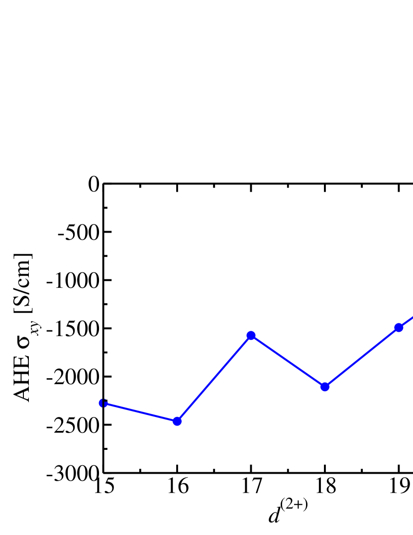
Figure 1: AHE conductivity $\sigma_{xy}$ vs. the prefactor $d^{(2+)}$ of the second moment potential.

In Ref. [15] we used $d^{(2+)}=15.0$ in order to reproduce the experimental bandwidth, exchange splitting, and position of the satellite peak. However, using $d^{(2+)}=20.0$ instead reproduces these experimental features also quite well, which we show in Fig. 2. In Ref. [16] we have found that the valence band satellite is in much better agreement with DMFT calculations and with experiment if the third moment potential is computed from the second moment potential using the constraint of the momentum distribution function of the UEG. However, since we have currently developed this procedure only for the UEG without spin-polarization we needed to apply a similar spin-polarization factor $\zeta^{t}_{\sigma}$ like in the present calculations. As a result, the spectral density of Ni in Ref. [16] matches experiment concerning the spin-polarization of the satellite peak, and the band width of the main band. However, it suffers from a similar overestimation of the exchange splitting as standard KS-DFT with LDA. In contrast, the present calculation yields the exchange-splitting close to experiments. Since the AHE depends strongly on the Fermi surface [23, 24, 25] we therefore use here the simpler approach of Eq. (24) instead of the improved approach of Ref. [16].

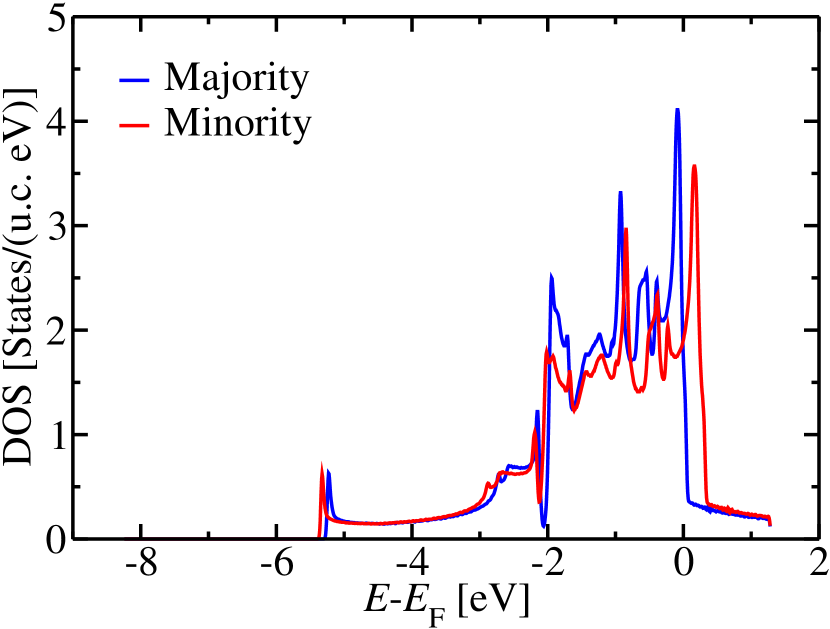
Figure 2: DOS in fcc Ni obtained from MFbSDFT.

V Summary

We describe the construction of Wannier functions from the first 4 spectral moment matrices. We show that these MLSMWFs can be used for the efficient interpolation of material property tensors such as the AHE within MFbSDFT. This paves the way for the application of MFbSDFT to compute response properties of materials. We demonstrate that MFbSDFT is able to reproduce the experimentally measured AHE in fcc Ni, similarly to LDA+$U$. Finally, we discuss that MLSMWFs may be computed also from the first 6 moments, and generally from the first $2P$ moments. This opens the perspective of using as many moments as necessary to reproduce all spectral features accurately in MFbSDFT.

References

- Marzari et al. [2012] N. Marzari, A. A. Mostofi, J. R. Yates, I. Souza, and D. Vanderbilt, Maximally localized wannier functions: Theory and applications, Rev. Mod. Phys. 84, 1419 (2012).
- Pizzi et al. [2020] G. Pizzi, V. Vitale, R. Arita, S. Blügel, F. Freimuth, G. Géranton, M. Gibertini, D. Gresch, C. Johnson, T. Koretsune, and et al., Wannier90 as a community code: new features and applications, J. Phys.: Condens. Matter 32, 165902 (2020).
- Yates et al. [2007] J. R. Yates, X. Wang, D. Vanderbilt, and I. Souza, Spectral and fermi surface properties from wannier interpolation, Phys. Rev. B 75, 195121 (2007).
- Wang et al. [2006] X. Wang, J. R. Yates, I. Souza, and D. Vanderbilt, Ab initio calculation of the anomalous hall conductivity by wannier interpolation, Phys. Rev. B 74, 195118 (2006).
- Pizzi et al. [2014] G. Pizzi, D. Volja, B. Kozinsky, M. Fornari, and N. Marzari, Boltzwann: A code for the evaluation of thermoelectric and electronic transport properties with a maximally-localized wannier functions basis, Computer Physics Communications 185, 422 (2014).
- Freimuth et al. [2014] F. Freimuth, S. Blügel, and Y. Mokrousov, Spin-orbit torques in co/pt(111) and mn/w(001) magnetic bilayers from first principles, Phys. Rev. B 90, 174423 (2014).
- Freimuth et al. [2015] F. Freimuth, S. Blügel, and Y. Mokrousov, Direct and inverse spin-orbit torques, Phys. Rev. B 92, 064415 (2015).
- Hanke et al. [2015] J.-P. Hanke, F. Freimuth, S. Blügel, and Y. Mokrousov, Higher-dimensional wannier functions of multiparameter hamiltonians, Phys. Rev. B 91, 184413 (2015).
- Hanke et al. [2020] J.-P. Hanke, F. Freimuth, B. Dupé, J. Sinova, M. Kläui, and Y. Mokrousov, Engineering the dynamics of topological spin textures by anisotropic spin-orbit torques, Phys. Rev. B 101, 014428 (2020).
- Hanke et al. [2018] J.-P. Hanke, F. Freimuth, S. Blügel, and Y. Mokrousov, Higher-dimensional wannier interpolation for the modern theory of the dzyaloshinskii–moriya interaction: Application to co-based trilayers, Journal of the Physical Society of Japan 87, 041010 (2018).
- Lihm and Park [2021] J.-M. Lihm and C.-H. Park, Wannier function perturbation theory: Localized representation and interpolation of wave function perturbation, Phys. Rev. X 11, 041053 (2021).
- Teale et al. [2022] A. M. Teale, T. Helgaker, A. Savin, C. Adano, B. Aradi, A. V. Arbuznikov, P. Ayers, E. J. Baerends, V. Barone, P. Calaminici, E. Cances, E. A. Carter, P. K. Chattaraj, H. Chermette, I. Ciofini, T. D. Crawford, F. D. Proft, J. Dobson, C. Draxl, T. Frauenheim, E. Fromager, P. Fuentealba, L. Gagliardi, G. Galli, J. Gao, P. Geerlings, N. Gidopoulos, P. M. W. Gill, P. Gori-Giorgi, A. Görling, T. Gould, S. Grimme, O. Gritsenko, H. J. A. Jensen, E. R. Johnson, R. O. Jones, M. Kaupp, A. Koster, L. Kronik, A. I. Krylov, S. Kvaal, A. Laestadius, M. P. Levy, M. Lewin, S. Liu, P.-F. cois Loos, N. T. Maitra, F. Neese, J. Perdew, K. Pernal, P. Pernot, P. Piecuch, E. Rebolini, L. Reining, P. Romaniello, A. Ruzsinszky, D. Salahub, M. Scheffler, P. Schwerdtfeger, V. N. Staroverov, J. Sun, E. Tellgren, D. J. Tozer, S. Trickey, C. A. Ullrich, A. Vela, G. Vignale, T. A. Wesolowski, X. Xu, and W. Yang, Dft exchange: Sharing perspectives on the workhorse of quantum chemistry and materials science, Physical chemistry chemical physics. (2022).
- Mandal et al. [2019] S. Mandal, K. Haule, K. M. Rabe, and D. Vanderbilt, Systematic beyond-dft study of binary transition metal oxides, npj Computational Materials 5, 115 (2019).
- Freimuth et al. [2022a] F. Freimuth, S. Blügel, and Y. Mokrousov, Construction of the spectral function from noncommuting spectral moment matrices, Phys. Rev. B 106, 045135 (2022a).
- Freimuth et al. [2022b] F. Freimuth, S. Blügel, and Y. Mokrousov, Moment functional based spectral density functional theory, Phys. Rev. B 106, 155114 (2022b).
- Freimuth et al. [2022c] F. Freimuth, S. Blügel, and Y. Mokrousov, Moment potentials for spectral density functional theory: Exploiting the momentum distribution of the uniform electron gas (2022c), arXiv:2212.12624 .
- Vogt et al. [2004] M. Vogt, R. Zimmermann, and R. J. Needs, Spectral moments in the homogeneous electron gas, Phys. Rev. B 69, 045113 (2004).
- Gori-Giorgi and Ziesche [2002] P. Gori-Giorgi and P. Ziesche, Momentum distribution of the uniform electron gas: Improved parametrization and exact limits of the cumulant expansion, Phys. Rev. B 66, 235116 (2002).
- Ortiz and Ballone [1994] G. Ortiz and P. Ballone, Correlation energy, structure factor, radial distribution function, and momentum distribution of the spin-polarized uniform electron gas, Phys. Rev. B 50, 1391 (1994).
- Ortiz and Ballone [1997] G. Ortiz and P. Ballone, Erratum: Correlation energy, structure factor, radial distribution function, and momentum distribution of the spin-polarized uniform electron gas [phys. rev. b 50, 1391 (1994)], Phys. Rev. B 56, 9970 (1997).
- Adamantopoulos et al. [2022] T. Adamantopoulos, M. Merte, D. Go, F. Freimuth, S. Blügel, and Y. Mokrousov, Laser-induced charge and spin photocurrents at the surface: A first-principles benchmark, Phys. Rev. Res. 4, 043046 (2022).
- Freimuth et al. [2021] F. Freimuth, S. Blügel, and Y. Mokrousov, Laser-induced torques in spin spirals, Phys. Rev. B 103, 054403 (2021).
- Haldane [2004] F. D. M. Haldane, Berry curvature on the fermi surface: Anomalous hall effect as a topological fermi-liquid property, Phys. Rev. Lett. 93, 206602 (2004).
- Wang et al. [2007] X. Wang, D. Vanderbilt, J. R. Yates, and I. Souza, Fermi-surface calculation of the anomalous hall conductivity, Phys. Rev. B 76, 195109 (2007).
- Vanderbilt et al. [2014] D. Vanderbilt, I. Souza, and F. D. M. Haldane, Comment on “weyl fermions and the anomalous hall effect in metallic ferromagnets”, Phys. Rev. B 89, 117101 (2014).
- Liebsch [1979] A. Liebsch, Effect of self-energy corrections on the valence-band photoemission spectra of ni, Phys. Rev. Lett. 43, 1431 (1979).
- Nolting et al. [1989] W. Nolting, W. Borgiel/, V. Dose, and T. Fauster, Finite-temperature ferromagnetism of nickel, Phys. Rev. B 40, 5015 (1989).
- Borgiel and Nolting [1990] W. Borgiel and W. Nolting, Many body contributions to the electronic structure of nickel, Zeitschrift für Physik B Condensed Matter 78, 241 (1990).
- Hamann and Vanderbilt [2009] D. R. Hamann and D. Vanderbilt, Maximally localized wannier functions for gw quasiparticles, Phys. Rev. B 79, 045109 (2009).
- Souza et al. [2001] I. Souza, N. Marzari, and D. Vanderbilt, Maximally localized wannier functions for entangled energy bands, Phys. Rev. B 65, 035109 (2001).
- Marzari and Vanderbilt [1997] N. Marzari and D. Vanderbilt, Maximally localized generalized wannier functions for composite energy bands, Phys. Rev. B 56, 12847 (1997).
- Weischenberg et al. [2011] J. Weischenberg, F. Freimuth, J. Sinova, S. Blügel, and Y. Mokrousov, Ab initio theory of the scattering-independent anomalous hall effect, Phys. Rev. Lett. 107, 106601 (2011).
- Weischenberg et al. [2013] J. Weischenberg, F. Freimuth, S. Blügel, and Y. Mokrousov, Scattering-independent anomalous nernst effect in ferromagnets, Phys. Rev. B 87, 060406 (2013).
- Fuh and Guo [2011] H.-R. Fuh and G.-Y. Guo, Intrinsic anomalous hall effect in nickel: A gga + study, Phys. Rev. B 84, 144427 (2011).
- Yang et al. [2001] I. Yang, S. Y. Savrasov, and G. Kotliar, Importance of correlation effects on magnetic anisotropy in fe and ni, Phys. Rev. Lett. 87, 216405 (2001).
- Freimuth et al. [2008] F. Freimuth, Y. Mokrousov, D. Wortmann, S. Heinze, and S. Blügel, Maximally localized wannier functions within the flapw formalism, Phys. Rev. B 78, 035120 (2008).
- Wang et al. [1996] X. Wang, R. Wu, D.-s. Wang, and A. J. Freeman, Torque method for the theoretical determination of magnetocrystalline anisotropy, Phys. Rev. B 54, 61 (1996).