EXIF as Language: Learning Cross-Modal
Associations Between Images and Camera Metadata

Abstract

We learn a visual representation that captures information about the camera that recorded a given photo. To do this, we train a multimodal embedding between image patches and the EXIF metadata that cameras automatically insert into image files. Our model represents this metadata by simply converting it to text and then processing it with a transformer. The features that we learn significantly outperform other self-supervised and supervised features on downstream image forensics and calibration tasks. In particular, we successfully localize spliced image regions “zero shot” by clustering the visual embeddings for all of the patches within an image.

Figure 1: (a) We learn a joint embedding between image patches and the EXIF metadata that cameras automatically insert into image files. Our model treats this metadata as a language-like modality: we convert the EXIF tags to text, concatenate them together, and then processes the result with a transformer. (b) We apply our representation to tasks that require understanding camera properties. For example, we can detect image splicing “zero shot” (and without metadata at test time) by finding inconsistent embeddings within an image. We show a manipulated image that contains content from two source photos. Since these photos were captured with different cameras, the two regions have dissimilar embeddings (visualized by PCA). We localize the splice by clustering the image’s patch embeddings.

1 Introduction

A major goal of the computer vision community has been to use cross-modal associations to learn concepts that would be hard to glean from images alone [2]. A particular focus has been on learning high level semantics, such as objects, from other rich sensory signals, like language and sound [59, 63]. By design, the representations learned by these approaches typically discard imaging properties, such as the type of camera that shot the photo, its lens, and the exposure settings, which are not useful for their cross-modal prediction tasks [18].

We argue that obtaining a complete understanding of an image requires both capabilities — for our models to perceive not only the semantic content of a scene, but also the properties of the camera that captured it. This type of low level understanding has proven crucial for a variety of tasks, from image forensics [34, 81, 53] to 3D reconstruction [35, 36], yet it has not typically been a focus of representation learning. It is also widely used in image generation, such as when users of text-to-image tools specify camera properties with phrases like “DSLR photo” [64, 60].

We propose to learn low level imaging properties from the abundantly available (but often neglected) camera metadata that is added to the image file at the moment of capture. This metadata is typically represented as dozens of Exchangeable Image File Format (EXIF) tags that describe the camera, its settings, and postprocessing operations that were applied to the image: e.g.,  Model: “iPhone 4s” or Focal Length: “35.0 mm”. We train a joint embedding through contrastive learning that puts image patches into correspondence with camera metadata (Fig. 1a). Our model processes the metadata with a transformer [76] after converting it to a language-like representation. To do this conversion, we take advantage of the fact that EXIF tags are typically stored in a human-readable (and text-based) format. We convert each tag to text, and then concatenate them together. Our model thus closely resembles contrastive vision-and-language models, such as CLIP [63], but with EXIF-derived text in place of natural language.

We show that our model can successfully estimate camera properties solely from images, and that it provides a useful representation for a variety of image forensics and camera calibration tasks. Our approaches to these tasks do not require camera metadata at test time. Instead, camera properties are estimated implicitly from image content via multimodal embeddings.

We evaluate the learned feature of our model on two classification tasks that benefit from a low-level understanding of images: estimating an image’s radial distortion parameter, and distinguishing real and manipulated images. We find that our features significantly outperform alternative supervised and self-supervised feature sets.

We also show that our embeddings can be used to detect image splicing “zero shot” (i.e., without labeled data), drawing on recent work [8, 55, 34] that detects inconsistencies in camera fingerprints hidden within image patches. Spliced images contain content from multiple real images, each potentially captured with a different camera and imaging pipeline. Thus, the embeddings that our model assigns to their patches, which convey camera properties, will have less consistency than those of real images. We detect manipulations by flagging images whose patch embeddings do not fit into a single, compact cluster. We also localize spliced regions by clustering the embeddings within an image (Fig. 1b).

We show through our experiments that:

• Camera metadata provides supervision for self-supervised representation learning.

• Image patches can be successfully associated with camera metadata via joint embeddings.

• Image-metadata embeddings are a useful representation for forensics and camera understanding tasks.

• Image manipulations can be identified “zero shot” by identifying inconsistencies in patch embeddings.

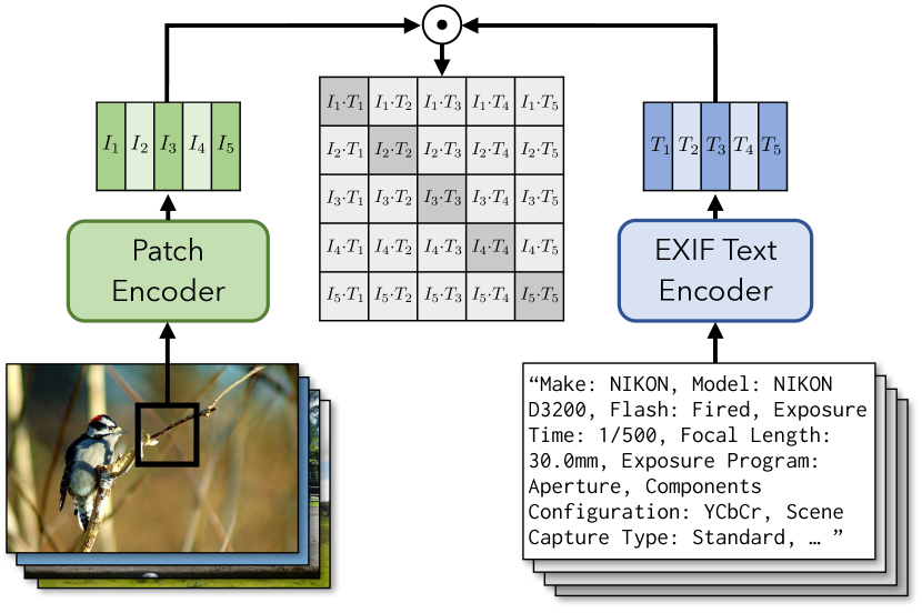
Figure 2: Cross-modal image and camera metadata model. We use contrastive learning to associate each image patch with the EXIF metadata that was extracted from its image file. We represent the metadata as text, which is obtained by concatenating the EXIF tags together. We then process it using a transformer.

2 Related Work

Estimating camera properties.

Camera metadata has been used for a range of tasks in computer vision, such as for predicting focal length [1, 72, 51, 32], performing white balancing [21, 50] and estimating camera models [75, 7, 40]. It has also been used as extra input for recognition tasks [73, 20]. Instead of estimating camera properties directly (which can be highly error prone [34]), our model predicts an embedding that distinguishes a patch’s camera properties from that of other patches in the dataset.

Image forensics.

Early work used physically motivated cues, such as misaligned JPEG blocks [22, 6], color filter array mismatches [24, 79, 3, 4], inconsistencies in noise patterns [48, 49, 62, 38], and compression or boundary artifacts [83, 33, 27, 5]. Other works use supervised learning methods [67, 41, 54, 86, 82, 81, 80, 77, 78, 65]. The challenge of collecting large datasets of fake images has led to alternative approaches, such as synthetic examples [54, 86, 82, 80]. Other work uses self-supervised learning, such as methods based on denoising [14], or that detect image manipulations by identifying image content that appears to come from different camera models [9, 7, 55]. Huh et al. [34] learned a patch similarity metric in two steps: they determined which EXIF tags are shared between the patches, then use these binary predictions as features for a second classifier that predicts whether two patches come from the same (or different) images. In contrast, we obtain a visual similarity metric that is well-suited to splice localization directly from our multimodal embeddings.

Language supervision in vision.

Recent works have obtained visual supervision from language. The formulation includes specific keyword prediction [56], bag-of-word multilabel classification [37], $n$-gram classification [47] and autoregressive language models [17, 69, 85]. Recently, Radford et al. [63] obtained strong performance by training a contrastive model on a large image-and-language dataset. Our technical approach is similar, but uses text from camera metadata in lieu of image captions.

Work in text-to-image synthesis often exploits camera information through prompting, such as by adding text like “DSLR photo of…” or “Sigma 500mm f/5” to prompts [60]. These methods, however, learn these camera associations through the (relatively rare) descriptions of cameras provided by humans, while ours learns them from an abundant and complementary learning signal, camera metadata.

3 Associating Images with Camera Metadata

We desire a visual representation that captures low level imaging properties, such as the settings of the camera that were used to shoot the photo. We then apply this learned representation to downstream tasks that require an understanding of camera properties.

3.1 Learning Cross-Modal Embeddings

We train a model to predict camera metadata from image content, thereby obtaining a representation that conveys camera properties. Following previous work in multimodal contrastive learning [63], we train a joint embedding between the two modalities, allowing our model to avoid the (error prone) task of directly predicting the attributes. Specifically, we want to jointly learn an image encoder and metadata encoder such that, given $N$ images and $N$ pieces of metadata information, the corresponding image–metadata pairs can be recognized by the model by maximizing embedding similarity. We use full-resolution image patches rather than resized images, so that our model can analyze low-level details that may be lost during downsampling.

Given a dataset of image patches and their corresponding camera metadata $\{(\mathbf{v}_{i},\mathbf{m}_{i})\}_{i=1}^{N}$, we learn visual and EXIF representations $f_{\theta}(\mathbf{v})$ and $g_{\phi}(\mathbf{m})$ by jointly training $f_{\theta}$ and $g_{\phi}$ using a contrastive loss [58]:

$$\mathcal{L}_{i}^{V,M}=-\log\frac{\exp{(f_{\theta}(\mathbf{v}_{i})\cdot g_{\phi}(\mathbf{m}_{i})/\tau)}}{\sum_{j=1}^{N}\exp(f_{\theta}(\mathbf{v}_{i})\cdot g_{\phi}(\mathbf{m}_{j})/\tau)},$$ (1)

where $\tau$ is a small constant. Following prior work [63], we define an analogous loss $\mathcal{L}^{M,V}$ that sums over visual (rather than metadata) examples in the denominator, and minimize a combined loss $\mathcal{L}=\mathcal{L}^{V,M}+\mathcal{L}^{M,V}$.

3.2 Representing the Camera Metadata

This formulation raises a natural question: how should we represent the metadata? The metadata within photos is stored as a set of EXIF tags, each indicating a different image property as shown in Table 1. EXIF tags span a range of formats and data types, and the set of tags that are present in a given photo can be highly inconsistent. Previous works that predict camera properties from images typically extract attributes of interest from the EXIF tags, and cast them to an appropriate data format — e.g., extracting a scalar-valued focal length category. This tag-specific processing limits the amount of metadata information that can be used as part of learning, and requires special-purpose architectures.

We exploit the fact that EXIF tags are typically stored in a human-readable format and can be straightforwardly converted to text (Fig. 2). This allows us to directly process camera metadata using models from natural language processing — an approach that has successfully been applied to processing various text-like inputs other than language, such as math [46] and code [11]. Specifically, we create a long piece of text from a photo’s metadata by converting each tag’s name and value to strings, and concatenating them together. We separate each tag name and value with a colon and space, and separate different tags with a space and comma. We evaluate a number of design decisions for this model in Sec. 4.4, such as the text format, choice of tags, and network architecture.

EXIF tag	Example values	#values
Camera Make	Canon, NIKON Corporation, Apple	312
Camera Model	NIKON D90, Canon EOS 7	3071
Software	Picasa, Adobe Photoshop, QuickTime	1711
Exposure Time	1/60 sec, 1/125 sec, 1/250 sec	2062
Focal Length	18.0 mm, 50.0 mm, 6.3 mm	931
Aperture Value	F2.8, F4, F5.6, F3.5	137
Scene Capture Type	Landscape, Portrait, Night Scene	5
Exposure Program	Aperture priority, Manual control	9
White Balance Mode	Auto, Manual	3
Thumbnail Compression	JPEG, Uncompressed	3
Digital Zoom Ratio	1, 1.5, 2, 1.2	49
ISO speed Ratings	100, 400, 300	460
Shutter Speed Value	1/60 sec, 1/63 sec, 1/124 sec	1161
Date/Time Digitized	2013:03:28 04:20:46	95932

Table 1: What information is contained within photo EXIF metadata? We list several of the most common EXIF tags, along with the common values and number of values they contain in the YFCC100M dataset [74].

3.3 Application: Zero-shot Image Forensics

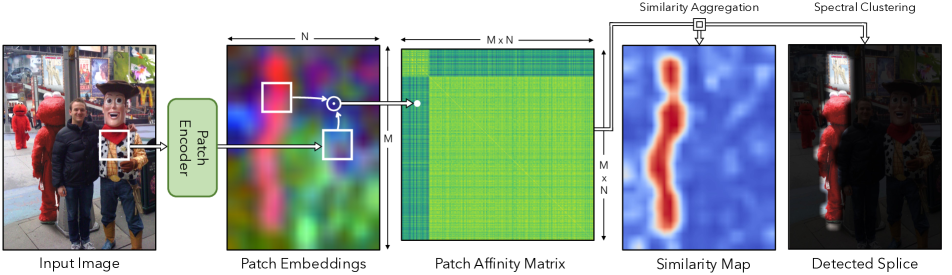
Figure 3: Zero shot splice localization. Given a spliced image (left), we compute our cross-modal embeddings for each image patch, which we visualize here using projections onto the top 3 principal components. We then compute the affinity matrix by taking dot product for every pair of patches. We localize the spliced region by clustering these embedding vectors.

After learning cross-modal representations from images and camera metadata, we can use them for downstream tasks that require an understanding of camera properties. One way to do this is by using the learned visual network features as a representation for classification tasks, following other work in self-supervised representation learning [30, 12]. We can also use our learned visual embeddings to perform “zero shot” image splice detection, by detecting inconsistencies in an input image’s imputed camera properties.

Spliced images are composed of regions from multiple real images. Since they are typically designed to fool humans, forensic models need to rely more on subtle (often non-semantic) cues to detect them. We got inspiration from Huh et al. [34], which predicts whether two image patches share the same camera properties. If two patches are predicted to have very different camera properties, then this provides evidence that they come from different images. In our work, we can naturally obtain this patch similarity by computing the dot product between two patches’ embeddings, since they have been trained to convey camera properties. We note that, unlike Huh et al. [34], we do not train a second, special-purpose classifier for this task, nor do we use augmentation to provide synthetic training examples (e.g., by applying different types of compression to the patches).

To determine whether an image is likely to contain a splice, we first compute an affinity matrix $A_{ij}=f_{\theta}(\mathbf{v}_{i})\cdot f_{\theta}(\mathbf{v}_{j})$ whose entries are the dot product between patches’ normalized embedding vectors. We score an image $\mathbf{v}$ using the sum of the exponentiated dot products between embeddings, $\phi(\mathbf{v})=\sum_{i,j}\exp(A_{ij}/\tau)$. This score indicates the likelihood that the image is unmodified, since high dot products indicate high similarity in imputed camera properties. To localize the spliced image regions within an image, we aggregate the similarity scores in $A_{ij}$ by clustering the rows using mean shift, following [34]. This results in a similarity map indicating the likelihood that each patch was extracted from the largest source photo that was used to create the composite. Alternatively, we can visualize the spliced region by performing spectral clustering via normalized cuts [34, 70], using $A_{ij}$ as an affinity matrix between patches. We visualize this approach in Fig. 3.

4 Results

4.1 Implementation

Architecture.

We use ResNet-50 pretrained on ImageNet as our image encoder. We found that the text encoder in models trained on captioning, such as CLIP [63], were not well-suited to our task, since they place low limits on the number of tokens. For the EXIF text encoder, we use DistilBERT [68] pretrained on Wikipedia and the Toronto Book Corpus [87]. We compute the feature representation of the EXIF as the activations for the end-of-sentence token from the last layer which is layer normalized and then linearly projected into multi-modal embedding space.

Training.

To train our model, we use 1.5M full-resolution images and EXIF pairs from a random subset of YFCC100M [74]. We discard images that have less than 10 of the EXIF tags. Because many images only have a small number of EXIF tags available, we only use tags that are present in more than half of these images. This results in 44 EXIF tags (see supplementary for the complete list). In contrast to other work [34], we do not rebalance the images to increase the rate of rare tags. During training, we randomly crop $124\times 124$ patches from high-resolution images. We use the AdamW optimizer [39] with a learning rate of $10^{-4}$, weight decay of $10^{-3}$, and mixed precision training. We use a cosine annealing learning rate schedule [52]. The batch size is set to 1024, and we train our model for 50 epochs.

Other model variations.

To study the importance of metadata supervision on the learned representation, we train a similar model that performs contrastive learning but does not use metadata. The model resembles image-image contrastive learning [88, 12, 30, 34], which has been shown to be highly effective for representation learning, and which may learn low-level camera information [18]. Different from typical contrastive learning approaches, we use strict cropping augmentation so that the views for our model (Eq. 1) come from different crops of the same image, to encourage it to learn low-level image features. We call this model CropCLR. Additionally, we evaluate a number of ablations of our model, including models that are trained with individual EXIF tags, that use different formats for the EXIF-derived text, and different network architectures (Table 5).

Models	Forensics				Radial Distortion
	CASIA I		CASIA II		Dresden	RAISE
	0.1pt10blackresize	0.1pt10blackcrop	0.1pt10blackresize	0.1pt10blackcrop	0.1pt10blackresize	0.1pt10blackresize
ImageNet pretrained	0.69	0.64	0.71	0.72	0.23	0.24
MoCo	0.67	0.67	0.68	0.69	0.24	0.28
CLIP	0.71	0.82	0.84	0.81	0.21	0.22
Ours - CropCLR	0.70	0.81	0.86	0.80	0.28	0.32
Ours - Full	0.75	0.85	0.87	0.84	0.31	0.35

Table 2: We do linear probing on top of learned representation to predict two camera related properties that are not presented in EXIF files. The good performance indicates that our model learns general imaging properties. resize  and crop  denote the image preprocessing applied.

4.2 Evaluating the learned features

First, we want to measure how well the learned features convey camera properties. Since EXIF file is already embedded with a lot of camera properties such as camera model, focal length, shuttle speed, etc., it should be unsurprising if we can predict those properties from images (we provide such results in Sec. 4.4). Instead, we want to study if the feature learned by the model can be generalized to other imaging properties that are not provided in the EXIF file. Specifically, we fit a linear classifier to our learned features on two prediction tasks: radial distortion estimation and forensic feature evaluation.

We compare the features from our image encoder with several other approaches, including supervised ImageNet pretraining [66], a state-of-the-art self-supervised model MoCo [30], CLIP [63], which obtains strong semantic representations using natural language supervision (rather than EXIF supervision), and finally the CropCLR variation of our model. To ensure a fair comparison, the backbone architectures for all approaches are the same (ResNet-50).

Radial distortion estimation.

Imperfections in camera lens production often lead to radial distortion artifacts in captured images. These artifacts are often removed as part of multi-view 3D reconstruction [71, 28], using methods that model distortion as a 4th-order polynomial of pixel position. Radial distortion is not typically specified directly by the camera metadata, and is thus often must be estimated through calibration [10], bundle adjustment [71], or from monocular cues [51].

We followed the evaluation setup of Lopez et al. [51], which estimates the quadratic term of the radial distortion model, $k_{1}$, directly from synthetically distorted images. This term can be used to provide an estimate of radial distortion that is sufficient for many tasks [61, 51]. We synthesized the $512\times 512$ images from the Dresden Image Database [26] and RAISE dataset [15] using $k_{1}$ parameters uniformly sampled in the range $[-0.4,0]$. To predict $k_{1}$, we used a regression-by-classification approach, quantizing the values of $k_{1}$ into 20 bins (We also show result in regression RMSE metrics in supplementary). We extracted features from different models, and trained a linear classifier on this 20-way classification problem. We provided them with a $512\times 512$ image as input, and obtained image features from the global average pooling layer after the final convolutional layer (i.e., the penultimate layer of a typical ResNet).

Representation learning for image forensics.

We evaluate our model’s ability to distinguish real and manipulated images. This is a task that requires a broader understanding of low level imaging properties, such as spotting unusual image statistics. We use the CASIA I [19] and CASIA II [44] datasets. The former contains only spliced fakes, while the latter contains a wider variety of manipulations. We again perform linear classification using the features provided by different models. We evaluate two types of preprocessing, resizing and center cropping, to test whether this low level task is sensitive to these details.

In both tasks, we found that our model’s features significantly outperformed those of the other models (Table 2). Our method achieves much better performance than traditional representational learning methods [31, 30, 63], perhaps because these models are encouraged to discard low-level details, while for our training task they are crucially important. Interestingly, the variation of our model that does not use EXIF metadata, CropCLR, outperforms the supervised [31] and self-supervised baselines [30], but significantly lags behind our full method. This is perhaps because it often suffices to use high-level cues (e.g. color histograms and object co-occurrence) to solve CropCLR’s pretext task. This suggests metadata supervision is an important learning signal and can effectively guide our model to learn general imaging information.

Style	Method	Columbia [57]		DSO [16]		RT [43]		In-the-Wild [34]		Hays [29]
		0.2pt10blackp-mAP	0.2pt10blackcIoU	0.2pt10blackp-mAP	0.2pt10blackcIoU	0.2pt10blackp-mAP	0.2pt10blackcIoU	0.2pt10blackp-mAP	0.2pt10blackcIoU	0.2pt10blackp-mAP	0.2pt10blackcIoU
Handcrafted	CFA [25]	0.76	0.75	0.24	0.46	0.40	0.63	0.27	0.45	0.22	0.45
	DCT [84]	0.43	0.41	0.32	0.51	0.12	0.50	0.41	0.51	0.21	0.47
	NOI [53]	0.56	0.47	0.38	0.50	0.19	0.50	0.42	0.52	0.27	0.47
Supervised	MantraNet [81]	0.78	0.88	0.53	0.78	0.50	0.54	0.50	0.63	0.27	0.56
	MAG [42]	0.69	0.77	0.48	0.56	0.51	0.55	0.47	0.59	0.30	0.61
	OSN [80]	0.68	0.90	0.55	0.85	0.51	0.81	0.66	0.88	0.28	0.57
Unsupervised	Noiseprint [14]	0.71	0.83	0.66	0.90	0.29	0.80	0.50	0.78	0.22	0.53
	EXIF-SC [34]	0.89	0.97	0.47	0.81	0.22	0.75	0.49	0.79	0.26	0.54
	Ours - CropCLR	0.87	0.96	0.48	0.81	0.23	0.74	0.47	0.80	0.26	0.55
	Ours - Full	0.92	0.98	0.56	0.85	0.23	0.74	0.51	0.82	0.30	0.58

Table 3: Zero shot splice localization. We evaluate our model on several datasets using permutation-invariant mean average precision (p-mAP) over pixels and class-balanced IOU (cIoU) with optimal threshold selected per image. The result indicates that our model is comparable to state-of-the-art methods, although not specially optimized for this task.

Dataset	Columbia [57]	DSO [16]	RT [43]
CFA [25]	0.83	0.49	0.54
DCT [84]	0.58	0.48	0.52
NOI [53]	0.73	0.51	0.52
EXIF-SC	0.98	0.61	0.55
Ours - CropCLR	0.96	0.62	0.52
Ours - Full	0.99	0.66	0.53

Table 4: Zero-shot splice detection: We compare our splice detection accuracy on 3 datasets. We measure the mean average precision (mAP) of detecting whether an image has been spliced.

4.3 Zero Shot Splice Detection and Localization

We evaluate our model on the task of detecting spliced images without any labeled training data. This is in contrast to Sec. 4.2, which used labeled data. We perform both splice detection (distinguish an image being spliced or not) and splice localization (localize spliced region within an image).

Implementation.

For fair evaluation, we closely follow the approach of Huh et al. [34]. Given an image, we sample patches in a grid, using a stride such that the number of patches sampled along the longest image dimension is 25. To increase the spatial resolution of each similarity map, we average the predictions of overlapping patches. We consider the smaller of the two detected regions to be the splice.

Evaluation.

In splice localization task, we compare our model to a variety of forensics methods. These include traditional methods that use handcrafted features [25, 84, 53], supervised methods [81, 42, 80], and self-supervised approaches [34, 14]. The datasets we use include Columbia [57], DSO [16], Realistic Tampering (RT) [43], In-the-Wild [34] and Hays and Efros inpainting images [29]. Columbia and DSO are created purely via image splicing, while Realistic Tampering contains a diverse set of manipulations. In-the-Wild is a splicing image dataset composed of internet images, which may also contain a variety of other manipulations. Hays and Efros [29] perform data-driven image inpainting. The quantitative comparison in terms of permuted-mAP (0.2pt10blackp-mAP) and class-balanced IoU (0.2pt10blackcIoU) following [34] are presented in Table 3. We also include splice image detection result in Table 8, where we compare our model to methods that enable splice detection.

Our model ranks first or second place for metrics in most datasets, and obtains performance comparable to top self-supervised methods that are specially designed for this task. In particular, our model significantly outperforms the most related technique, EXIF-SC [34]. We note that both our method and EXIF-SC get relatively low performance on the Realistic Tampering dataset. This may be due to the fact that this dataset contains manipulations such as copy-move that we do not expect to detect (since both regions share the same camera properties). In contrast to methods based on segmentation [81, 80, 14], we do not aim to have spatially precise matches, and output relatively low-resolution localization maps based on large patches. Consequently, our model is not well-suited to detecting very small splices, which also commonly occur in the Realistic Tampering dataset.

In Fig. 4, we show qualitative results, including both similarity maps and spectral clustering results. In Fig. 6, we compare our model with those of several other techniques. Interestingly, EXIF-SC has false positives in overexposed regions (as pointed out by [34]), since its classifier cannot infer whether these regions are (or are not) part of the rest of the scene. In contrast, our model successfully handles these regions. CropCLR incorrectly flags regions that are semantically different from the background, because this is a strong indication that the patches come from different images. In contrast, we successfully handle these cases, since our model has no such “shortcut” in its learning task.

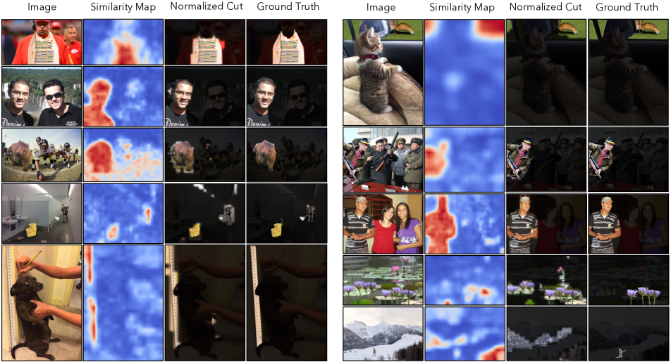
Figure 4: Qualitative visualization of splice localization result. We also include two typical scenarios where our model fails: copy-move tampering and very small splicing region (last two rows in right column).

	Method	EXIF	Radial	Forens.
	Majority class baseline	0.12	0.05	0.50
Supervision	All EXIF tags	0.35	0.29	0.85
	CropCLR	0.29	0.22	0.84
	“Camera Model” tag only	0.31	0.27	0.80
	“Color Space” tag only	0.12	0.12	0.61
	YFCC image descriptions	0.15	0.16	0.70
Tag format	Fixed order, w/ tag name	0.35	0.29	0.85
	Fixed order, w/o tag name	0.35	0.28	0.86
	Rand. order, w/ tag name	0.34	0.26	0.77
	Rand. order, w/o tag name	0.33	0.26	0.76
Architecture	DistilBERT, w/ pretrained	0.35	0.29	0.85
	DistilBERT, w/o pretrained	0.36	0.25	0.77
	ALBERT, w/ pretrained	0.33	0.29	0.84
	ALBERT, w/o pretrained	0.34	0.26	0.79

Table 5: Model ablations. Downstream accuracy for versions of the model trained with different text supervision, representations of camera metadata, and architectures. We use linear probing to evaluate the average prediction accuracy of EXIF tag values on our YFCC test set, radial distortion estimation on Dresden dataset, and real-or-fake classification on CASIA I dataset. Rows with gray background (replicated for ease of comparison) represent the same model which is our “full” model.

4.4 Ablation Study

To help understand which aspects of our approach are responsible for its performance, we evaluated a variety of variations of our model, including different training supervision, representations for the camera metadata, and network architectures.

We evaluated each model’s features quality using linear probing on the radial distortion estimation and splice detection task (same as Sec. 4.2). As an additional evaluation, we classify the values of common EXIF tags by applying linear classifiers to our visual representation. We convert the values of each EXIF tag into discrete categories, by quantizing common values and removing examples that do not fit into any category. We average prediction accuracies over $44$ EXIF tags to obtain overall accuracy. We provide more details in the supplementary. All models were trained for 30 epochs on 800K images on a subset of YFCC100M dataset. The associated texts are obtained from the image descriptions and EXIF data provided by the dataset.

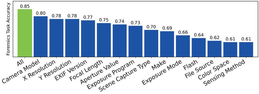
Figure 5: Per-tag forensics task accuracy. We train various models supervised by individual EXIF tags, then evaluate the learned representations for splice detection task on CASIA I.

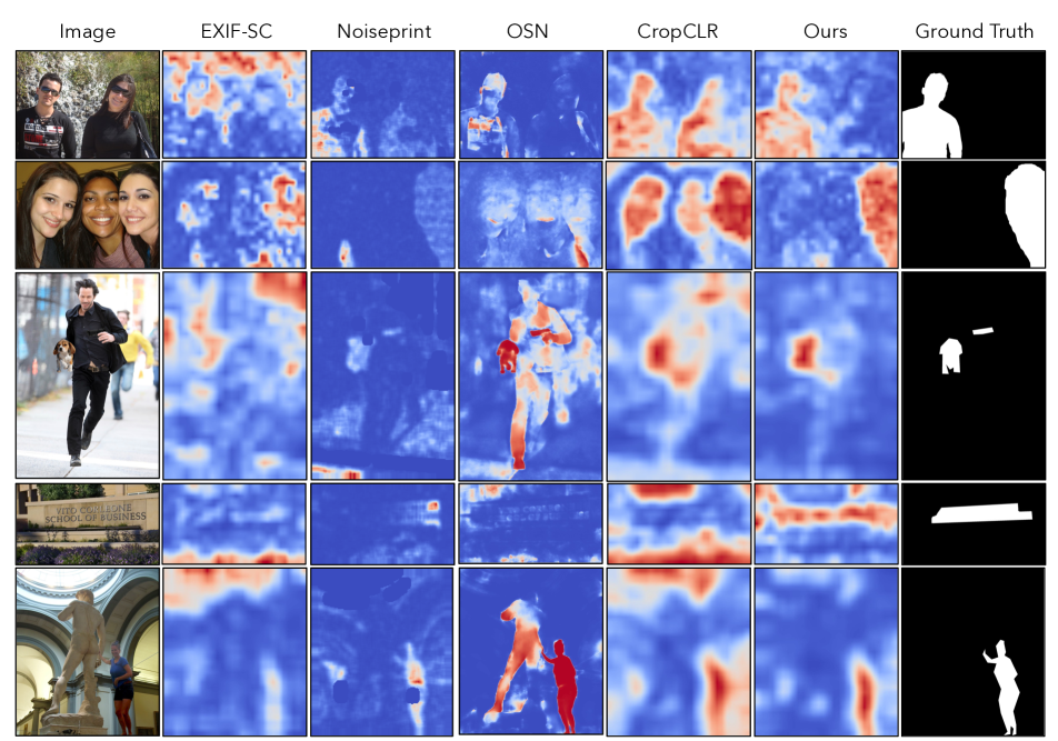
Figure 6: Qualitative comparison to other methods. Our method can correctly localize splices in many scenarios where other methods fail. For example, EXIF-SC [34] fails on overexposed image regions; OSN [80] and CropCLR often segment scenes based on semantics.

Metadata supervision.

We evaluate a variation of our model that trains using the image descriptions provided by YFCC100M in lieu of camera metadata, as well as models supervised by individual EXIF tags (Table 5). For the variations supervised by a single EXIF tag, we chose $14$ common tags for this experiment, training a separate network for each one. The results of the per-tag evaluation is shown in Fig. 5. These results suggest that having access to the full metadata provides significantly better performance than using individual tags. Moreover, there is a wide variation in the performance of models that use different tag. This may be because the high performing tags, such as Camera Model, convey significantly more information about the full range of camera properties than others, such as Color Space and Sensing Method. These results suggest that a model that simply uses the full range of tags can extract significantly more camera information from the metadata. We also found that the variation trained on image descriptions (rather than EXIF text) performed significantly worse than other models.

Tag format.

Since EXIF does not have a natural order of tags, we ask what will happen if we randomize the EXIF tag order during training. Table 5 shows the performance drops for all three evaluations in this case. This may be due to the fact that the Transformer model is forced to learn meaningful positional embeddings corresponding to each EXIF tag if their order keeps on changing. We also tried removing the tag names from the camera metadata and just provide the values for those keys, e.g. replacing Make: Apple with Apple. Interestingly, this model performs on par with the model that has tag names, suggesting that the network can discern information about the tags from the values alone.

Text encoder architecture.

To test whether performance of our model tied to a specific transformer architecture, we experimented with two different transformer models, DistilBERT [68] and ALBERT [45]. We see that both architectures obtain similar performance on all three tasks with DistilBERT slightly outperforming ALBERT. We also test how much pretraining the text encoder helps with the performance. From Table 5, we can see pretraining improves performance on the radial distortion and forensics tasks.

5 Discussion

In this paper, we proposed to learn camera properties by training models to find cross-modal correspondences between images and camera metadata. To achieve this, we created a model that exploits the fact that EXIF metadata can easily be represented and processed as text. Our model achieves strong performance amongst self-supervised methods on a variety of downstream tasks that require understanding camera properties, including zero shot image forensics and radial distortion estimation. We see our work opening several possible directions. First, it opens the possibility of creating multimodal learning systems that use camera metadata as another form of supervision, providing complementary information to high-level modalities like language and sound. Second, it opens applications that require an understanding of low level sensor information, which may benefit from our feature sets.

Limitations and Broader Impacts.

We have shown that our learned features are useful for image forensics, which has potential to reduce the spread of disinformation [23]. The model that we will release may not be fully representative of the cameras in the wild, since it was trained only on photos available in the YFCC100M datatset [74].

Acknowledgements.

We thank Alexei Efros for the helpful discussions. This research was developed with funding from the Defense Advanced Research Projects Agency (DARPA) under Contract No. HR001120C0123. The views, opinions and/or findings expressed are those of the author and should not be interpreted as representing the official views or policies of the Department of Defense or the U.S. Government.

Appendix A Additional ablations

We also experiment with different types of patch encoders and initialized them from different pretraining models. The experimental settings are exactly the same as Sec. 4.4. ResNet-50 outperforms ViT-B/32, while the results are not significantly affected by pretraing.

Patch encoder	EXIF	Radial	Forens.
ImageNet pretrained + ViT-B/32	0.32	0.27	0.85
ImageNet pretrained + ResNet-50	0.35	0.29	0.85
CLIP pretrained + ViT-B/32	0.31	0.28	0.84
CLIP pretrained + ResNet-50	0.34	0.29	0.85

Table 6: Additional architecture and pretraining configurations.

Appendix B Sensitivity to Image Compression

We test the robustness of JPEG compression for different models in the zero-shot splice localization task (Fig. 7). We use in the wild as testing dataset. All methods perform worse when noise is added which is common in forensics tasks.

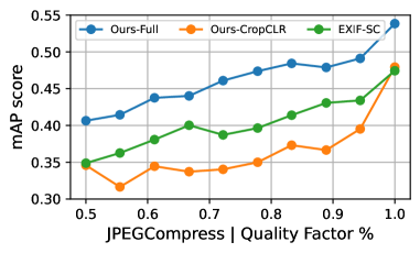
Figure 7: Effect of Splice localization vs. JPEG compression on In the Wild.

Appendix C Experimental Details

We provide additional experimental details about the downstream tasks.

C.1 Radial Distortion Model

We follow the radial distortion model proposed in Lopez et al. [51]. Let $(x,y)$ represent the normalized image pixel coordinate. Radial distortion can be modeled as scaling the normalized coordinates by a factor of $d$, which is a function of the distance from pixel location to center of image $r$ and distortion parameters $k_{1}$ and $k_{2}$:

$$d=1+k_{1}r^{2}+k_{2}r^{4}$$ (2)

and set $\left(x_{d},y_{d}\right)=(dx,dy)$. Since the relationship between $k_{1}$ and $k_{2}$ can be approximated modeled as [51]:

$$k_{2}=0.019k_{1}+0.805k_{1}^{2},$$ (3)

aim to predict only $k_{1}$.

To address the concern about sparsity of discrete bins we used in Table 2, we provide another set of experiments in which we finetune and regress distortion via L2 loss. The result in terms of root mean square error (RMSE) are provided in Table 7. The finding is consistent with Table 2 that we outperform other weights.

Dataset	Dresden	RAISE
ImageNet pretrained	0.11	0.12
MoCo	0.12	0.11
CLIP	0.10	0.11
Ours - CropCLR	0.06	0.08
Ours - Full	0.06	0.04

Table 7: Radial distortion regression (RMSE error)

C.2 EXIF Prediction Application

We provide implementation details for the downstream application of predicting EXIF tags from visual features (Sec. 4.2). To formulate the problem as a classification task, we convert the values of each EXIF tag into discrete categories, using the following rules: if an EXIF tag has less than 20 distinct values, we use each value as a class. For example, the white balance mode tag has only two values auto, manual, each of which becomes a category. If an EXIF tag has continuous values (e.g., focal length) or more than 20 discrete value (e.g., camera model), we will quantize its common values to a set of bins using hand-chosen rules, and remove examples that do not fit into any category. For example, for the camera model tag, which holds a sparse set of camera models, we merge their value according to their brand (value NIKON D90 will fall into NIKON category). We define common values to be those that occur with probability greater than 0.1% in the dataset.

C.3 Linear Probing Implementation Details

The linear probing experiment set up is as follows: We follow the approach from Chen et al. [13]. We use Adam optimizer with no weight decay, and set learning rate to be $0.01$ and optimizer momentum to be $\beta_{1},\beta_{2}=0.9,0.95$. We also normalize the image features before providing them to the linear classifier. We use a batch size of 1024, and we train the classifier for 20 epochs.

Appendix D Confusion Plot

We ask how the performance of a model trained using a specific tag performs when it is tasked with predicting the value of other tags. This may indicate the generalizability of the training tag. We therefore take the per-tag models (same as Fig. 5) and measure their prediction accuracies of different tag values (see Fig. 8). The result shows models trained on some tags may contain useful information to be generalized to other tags, such as the model trained with “camera make” performs well in “camera model” and “aperture” predictions. In contrast, that model trained on tags that don’t have rich values or information (like Flash) can not generalize to other tags well.

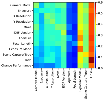
Figure 8: Confusion matrix of EXIF tag prediction accuracy. Each model is trained on one tag and tasked with predicting another tag. Each row corresponds to a model trained with a single tag, and each column represents the prediction accuracy for another tag.

Appendix E EXIF Metadata Analysis

In this section, we provide a detailed analysis of EXIF metadata information in both the training and testing datasets. We hope this could help readers understand more about the characteristic of EXIF data.

E.1 Complete list of EXIF tags used in training

We present the complete list of EXIF tags being used by our model in Table 9, along with representative values and the total number of values.

E.2 Metadata in downstream tasks

We analyze the distribution of metadata that is provided in each evaluation set, and compare it to the tags in our YFCC training set (Table 8). First, we found that most of the metadata tags are not available in testing datasets because they are often removed for privacy reasons. However, the performance of our model will not be affected by this issue since it does not require metadata at test time. Second, for the tags that are available in testing datasets, nearly all the values have appeared in training time, indicating the diversity of training data.

Dataset	Available metadata and tag counts	Values missing in training
Dresden	Camera Model (73), WH (12), Flash (2)	All included (0)
RAISE	Camera Model (3), WH (3), Color Space (2)	“Color Space: Adobe RGB” (1)
CASIA I & II	All missing	–
DSO	WH (5)	All included (0)
Columbia	Camera Model (4), WH (2)	All included (0)
RT	Camera Model (4), WH (1)	All included (0)
Hays	Camera Model (4), WH (3)	All included (0)
In the Wild	WH (64)	Various WH (17)

Table 8: Downstream metadata distribution (WH = Width/Height tags, distinct values per tag in parentheses).

EXIF tag	Example values	# values
Aperture Value	F2.8, F4, F5.6, F3.5	137
Camera Make	Canon, NIKON Corporation, Apple	312
Camera Model	NIKON D90, Canon EOS 7	3071
Color Space	sRGB, Undefined	3
Components Configuration	YCbCr, CrCbY	10
Compressed Bits	4 bits per pixel	6
Custom Rendered	Custom process, Normal process	3
Data/Time	2013:03:28 04:20:46	95982
Data/Time Digitized	2013:03:28 04:20:46	95932
Data/Time Original	2013:03:28 04:20:46	95839
Digital Zoom Ratio	1, 1.5, 2, 1.2	49
Exif Image Height	2592 pixels, 2304 pixels	3325
Exif Image Width	2592 pixels, 2408 pixels	3787
Exif Version	2.21, 2.20, 2.30	14
Exposure Bias Value	0 EV, -1 EV, 1 EV	71
Exposure Mode	Auto exposure, Manual exposure	4
Exposure Program	Aperture priority, Manual control	9
Exposure Time	1/60 sec, 1/125 sec, 1/250 sec	2062
F-Number	F2.8, F5.6, F4	150
File Source	Digital Still Camera, Print Scanner	6
Flash	Unfired, Fired(red-eye reduction)	20
FlashPix Version	1.00, 0.10, 1.01	14
Focal Length	18.0 mm, 50.0 mm, 6.3 mm	931
Focal Place X Resolution	292 dots per inch	61
Focal Place Y Resolution	292 dots per inch	60
Gain Control	Low, High	2
ISO Speed Ratings	100, 400, 300	460
Interoperability Index	0, unknown	2
Interoperability Version	1.00, 1.10, 30.00	16
Max Aperture Value	F2.8, F3.5, F4	81
Metering Mode	Multi-segment, Spot, average	8
Orientation	Top, right side (Mirror horizontal)	2
Resolution Unit	Inch, cm	3
Scene Capture Type	Landscape, Portrait, Night Scene	5
Sensing Method	One-Chip color area sensor	4
Shutter Speed Value	1/60 sec, 1/63 sec, 1/124 sec	1161
Software	Picasa, Adobe Photoshop, QuickTime	1711
Thumbnail Compression	JPEG, Uncompressed	3
Thumbnail Length	0 bytes, 16712 bytes	17743
Thumbnail Offset	5108 bytes, 9716 bytes	11298
White Balance Mode	Auto, Manual	3
X Resolution	72 dots per inch	62
Y Resolution	72 dots per inch	64
YCbCr Positioning	datum point, Center of pixel array	3

Table 9: Full list of EXIF tags being used in training. This extends the list from Table 1 in the main paper.

Appendix F Additional Qualitative Results

We provide additional qualitative results for our zero-shot splice localization model. In Fig. 9 and Fig. 10 (left), we show accurate predictions. In Fig. 10 (right), we show failure cases.

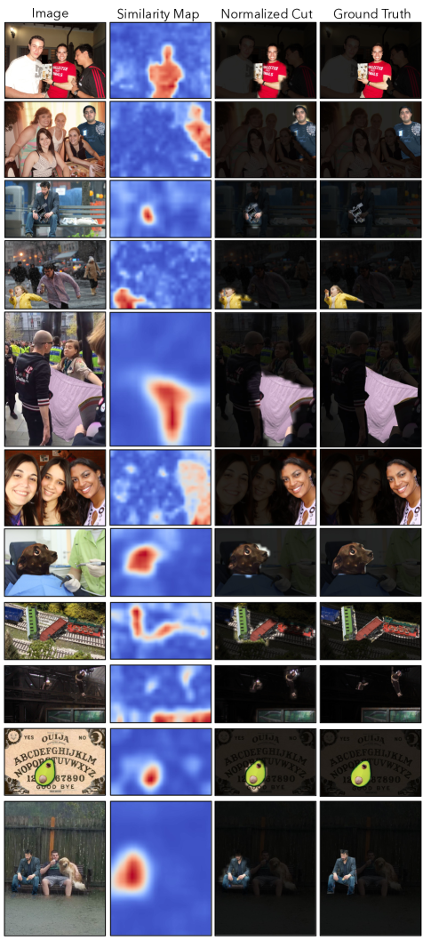
Figure 9: Additional zero-shot splice localization results.

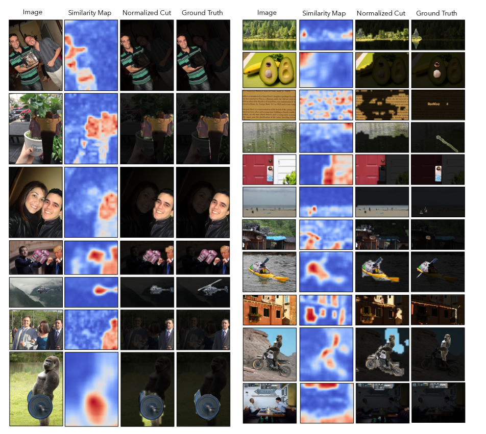
Figure 10: Additional zero-shot splice localization results: success cases (left) and failure cases (right).

References

- [1] Ali Azarbayejani and Alex P Pentland. Recursive estimation of motion, structure, and focal length. IEEE Transactions on Pattern Analysis and Machine Intelligence, 17(6):562–575, 1995.
- [2] Tadas Baltrušaitis, Chaitanya Ahuja, and Louis-Philippe Morency. Multimodal machine learning: A survey and taxonomy. IEEE transactions on pattern analysis and machine intelligence, 41(2):423–443, 2018.
- [3] Quentin Bammey, Rafael Grompone von Gioi, and Jean-Michel Morel. An adaptive neural network for unsupervised mosaic consistency analysis in image forensics. In Proceedings of the IEEE/CVF Conference on Computer Vision and Pattern Recognition, pages 14194–14204, 2020.
- [4] Quentin Bammey, Rafael Grompone von Gioi, and Jean-Michel Morel. An adaptive neural network for unsupervised mosaic consistency analysis in image forensics. In Proceedings of the IEEE/CVF Conference on Computer Vision and Pattern Recognition, pages 14194–14204, 2020.
- [5] Jawadul H Bappy, Amit K Roy-Chowdhury, Jason Bunk, Lakshmanan Nataraj, and BS Manjunath. Exploiting spatial structure for localizing manipulated image regions. In Proceedings of the IEEE international conference on computer vision, pages 4970–4979, 2017.
- [6] Tiziano Bianchi and Alessandro Piva. Image forgery localization via block-grained analysis of jpeg artifacts. IEEE Transactions on Information Forensics and Security, 7(3):1003–1017, 2012.
- [7] Luca Bondi, Luca Baroffio, David Güera, Paolo Bestagini, Edward J Delp, and Stefano Tubaro. First steps toward camera model identification with convolutional neural networks. IEEE Signal Processing Letters, 24(3):259–263, 2016.
- [8] Luca Bondi, Silvia Lameri, David Güera, Paolo Bestagini, Edward J Delp, and Stefano Tubaro. Tampering detection and localization through clustering of camera-based cnn features. In 2017 IEEE Conference on Computer Vision and Pattern Recognition Workshops (CVPRW), 2017.
- [9] Luca Bondi, Silvia Lameri, David Guera, Paolo Bestagini, Edward J Delp, Stefano Tubaro, et al. Tampering detection and localization through clustering of camera-based cnn features. In CVPR Workshops, volume 2, 2017.
- [10] J-Y Bouguet. Camera calibration toolbox for matlab. http://www. vision. caltech. edu/bouguetj/calib_doc/index. html, 2004.
- [11] Mark Chen, Jerry Tworek, Heewoo Jun, Qiming Yuan, Henrique Ponde de Oliveira Pinto, Jared Kaplan, Harri Edwards, Yuri Burda, Nicholas Joseph, Greg Brockman, et al. Evaluating large language models trained on code. arXiv preprint arXiv:2107.03374, 2021.
- [12] Ting Chen, Simon Kornblith, Mohammad Norouzi, and Geoffrey Hinton. A simple framework for contrastive learning of visual representations. In International conference on machine learning, pages 1597–1607. PMLR, 2020.
- [13] Xinlei Chen, Saining Xie, and Kaiming He. An empirical study of training self-supervised vision transformers. In Proceedings of the IEEE/CVF International Conference on Computer Vision, pages 9640–9649, 2021.
- [14] Davide Cozzolino and Luisa Verdoliva. Noiseprint: a cnn-based camera model fingerprint. IEEE Transactions on Information Forensics and Security, 15:144–159, 2019.
- [15] Duc-Tien Dang-Nguyen, Cecilia Pasquini, Valentina Conotter, and Giulia Boato. Raise: A raw images dataset for digital image forensics. In Proceedings of the 6th ACM multimedia systems conference, pages 219–224, 2015.
- [16] Tiago José De Carvalho, Christian Riess, Elli Angelopoulou, Helio Pedrini, and Anderson de Rezende Rocha. Exposing digital image forgeries by illumination color classification. IEEE Transactions on Information Forensics and Security, 8(7):1182–1194, 2013.
- [17] Karan Desai and Justin Johnson. Virtex: Learning visual representations from textual annotations. In Proceedings of the IEEE/CVF conference on computer vision and pattern recognition, pages 11162–11173, 2021.
- [18] Carl Doersch, Abhinav Gupta, and Alexei A Efros. Unsupervised visual representation learning by context prediction. In Proceedings of the IEEE international conference on computer vision, pages 1422–1430, 2015.
- [19] Jing Dong, Wei Wang, and Tieniu Tan. CASIA image tampering detection evaluation database. In 2013 IEEE China Summit and International Conference on Signal and Information Processing. IEEE, July 2013.
- [20] Jiayuan Fan, Hong Cao, and Alex C Kot. Estimating exif parameters based on noise features for image manipulation detection. IEEE Transactions on Information Forensics and Security, 8(4):608–618, 2013.
- [21] Jiayuan Fan, Tao Chen, and Alex ChiChung Kot. Exif-white balance recognition for image forensic analysis. Multidimensional Systems and Signal Processing, 28(3):795–815, 2017.
- [22] Hany Farid. Exposing digital forgeries from jpeg ghosts. IEEE transactions on information forensics and security, 4(1):154–160, 2009.
- [23] Hany Farid. Photo forensics. MIT Press, 2016.
- [24] Pasquale Ferrara, Tiziano Bianchi, Alessia De Rosa, and Alessandro Piva. Image forgery localization via fine-grained analysis of cfa artifacts. IEEE Transactions on Information Forensics and Security, 7(5):1566–1577, 2012.
- [25] Pasquale Ferrara, Tiziano Bianchi, Alessia De Rosa, and Alessandro Piva. Image forgery localization via fine-grained analysis of cfa artifacts. IEEE Transactions on Information Forensics and Security, 7(5):1566–1577, 2012.
- [26] Thomas Gloe and Rainer Böhme. The’dresden image database’for benchmarking digital image forensics. In Proceedings of the 2010 ACM symposium on applied computing, pages 1584–1590, 2010.
- [27] Ashima Gupta, Nisheeth Saxena, and SK Vasistha. Detecting copy move forgery using dct. International Journal of Scientific and Research Publications, 3(5):1, 2013.
- [28] Richard Hartley and Andrew Zisserman. Multiple view geometry in computer vision. Cambridge university press, 2003.
- [29] James Hays and Alexei A Efros. Scene completion using millions of photographs. ACM Transactions on Graphics (ToG), 26(3):4–es, 2007.
- [30] Kaiming He, Haoqi Fan, Yuxin Wu, Saining Xie, and Ross Girshick. Momentum contrast for unsupervised visual representation learning. In Proceedings of the IEEE/CVF conference on computer vision and pattern recognition, pages 9729–9738, 2020.
- [31] Kaiming He, Xiangyu Zhang, Shaoqing Ren, and Jian Sun. Deep residual learning for image recognition. In Proceedings of the IEEE conference on computer vision and pattern recognition, pages 770–778, 2016.
- [32] Yannick Hold-Geoffroy, Kalyan Sunkavalli, Jonathan Eisenmann, Matthew Fisher, Emiliano Gambaretto, Sunil Hadap, and Jean-François Lalonde. A perceptual measure for deep single image camera calibration. In Proceedings of the IEEE Conference on Computer Vision and Pattern Recognition, pages 2354–2363, 2018.
- [33] Wu-Chih Hu and Wei-Hao Chen. Effective forgery detection using dct+ svd-based watermarking for region of interest in key frames of vision-based surveillance. International Journal of Computational Science and Engineering, 8(4):297–305, 2013.
- [34] Minyoung Huh, Andrew Liu, Andrew Owens, and Alexei A Efros. Fighting fake news: Image splice detection via learned self-consistency. In ECCV, 2018.
- [35] Shahram Izadi, David Kim, Otmar Hilliges, David Molyneaux, Richard Newcombe, Pushmeet Kohli, Jamie Shotton, Steve Hodges, Dustin Freeman, Andrew Davison, et al. Kinectfusion: real-time 3d reconstruction and interaction using a moving depth camera. In Proceedings of the 24th annual ACM symposium on User interface software and technology, pages 559–568, 2011.
- [36] Michael R James and Stuart Robson. Straightforward reconstruction of 3d surfaces and topography with a camera: Accuracy and geoscience application. Journal of Geophysical Research: Earth Surface, 117(F3), 2012.
- [37] Armand Joulin, Laurens van der Maaten, Allan Jabri, and Nicolas Vasilache. Learning visual features from large weakly supervised data. In European Conference on Computer Vision, pages 67–84. Springer, 2016.
- [38] Thibaut Julliand, Vincent Nozick, and Hugues Talbot. Image noise and digital image forensics. In International Workshop on Digital Watermarking, pages 3–17. Springer, 2015.
- [39] Diederik P Kingma and Jimmy Ba. Adam: A method for stochastic optimization. arXiv preprint arXiv:1412.6980, 2014.
- [40] Matthias Kirchner and Thomas Gloe. Forensic camera model identification. Handbook of Digital Forensics of Multimedia Data and Devices, pages 329–374, 2015.
- [41] Vladimir V Kniaz, Vladimir Knyaz, and Fabio Remondino. The point where reality meets fantasy: Mixed adversarial generators for image splice detection. Advances in Neural Information Processing Systems, 32, 2019.
- [42] Vladimir V Kniaz, Vladimir Knyaz, and Fabio Remondino. The point where reality meets fantasy: Mixed adversarial generators for image splice detection. Advances in Neural Information Processing Systems, 32, 2019.
- [43] Paweł Korus and Jiwu Huang. Multi-scale analysis strategies in prnu-based tampering localization. IEEE Transactions on Information Forensics and Security, 12(4):809–824, 2016.
- [44] Akash Kumar and Arnav Bhavsar. Copy-move forgery classification via unsupervised domain adaptation. arXiv preprint arXiv:1911.07932, 2019.
- [45] Zhenzhong Lan, Mingda Chen, Sebastian Goodman, Kevin Gimpel, Piyush Sharma, and Radu Soricut. Albert: A lite bert for self-supervised learning of language representations. arXiv preprint arXiv:1909.11942, 2019.
- [46] Aitor Lewkowycz, Anders Andreassen, David Dohan, Ethan Dyer, Henryk Michalewski, Vinay Ramasesh, Ambrose Slone, Cem Anil, Imanol Schlag, Theo Gutman-Solo, et al. Solving quantitative reasoning problems with language models. arXiv preprint arXiv:2206.14858, 2022.
- [47] Ang Li, Allan Jabri, Armand Joulin, and Laurens Van Der Maaten. Learning visual n-grams from web data. In Proceedings of the IEEE International Conference on Computer Vision, pages 4183–4192, 2017.
- [48] Bo Liu and Chi-Man Pun. Splicing forgery exposure in digital image by detecting noise discrepancies. International Journal of Computer and Communication Engineering, 4(1):33, 2015.
- [49] Bo Liu, Chi-Man Pun, and Xiao-Chen Yuan. Digital image forgery detection using jpeg features and local noise discrepancies. The Scientific World Journal, 2014, 2014.
- [50] Yung-Cheng Liu, Wen-Hsin Chan, and Ye-Quang Chen. Automatic white balance for digital still camera. IEEE Transactions on Consumer Electronics, 41(3):460–466, 1995.
- [51] Manuel Lopez, Roger Mari, Pau Gargallo, Yubin Kuang, Javier Gonzalez-Jimenez, and Gloria Haro. Deep single image camera calibration with radial distortion. In Proceedings of the IEEE/CVF Conference on Computer Vision and Pattern Recognition, pages 11817–11825, 2019.
- [52] Ilya Loshchilov and Frank Hutter. Sgdr: Stochastic gradient descent with warm restarts. arXiv preprint arXiv:1608.03983, 2016.
- [53] Babak Mahdian and Stanislav Saic. Using noise inconsistencies for blind image forensics. Image and Vision Computing, 27(10):1497–1503, 2009.
- [54] Francesco Marra, Diego Gragnaniello, Luisa Verdoliva, and Giovanni Poggi. A full-image full-resolution end-to-end-trainable cnn framework for image forgery detection. IEEE Access, 8:133488–133502, 2020.
- [55] Owen Mayer and Matthew C Stamm. Learned forensic source similarity for unknown camera models. In ICASSP, 2018.
- [56] Yasuhide Mori, Hironobu Takahashi, and Ryuichi Oka. Image-to-word transformation based on dividing and vector quantizing images with words. In First international workshop on multimedia intelligent storage and retrieval management, pages 1–9. Citeseer, 1999.
- [57] Tian-Tsong Ng, Shih-Fu Chang, and Q Sun. A data set of authentic and spliced image blocks. Columbia University, ADVENT Technical Report, pages 203–2004, 2004.
- [58] Aaron van den Oord, Yazhe Li, and Oriol Vinyals. Representation learning with contrastive predictive coding. arXiv preprint arXiv:1807.03748, 2018.
- [59] Andrew Owens and Alexei A Efros. Audio-visual scene analysis with self-supervised multisensory features. In Proceedings of the European Conference on Computer Vision (ECCV), pages 631–648, 2018.
- [60] Guy Parsons. Dall-e 2 prompt book. http://dallery.gallery/wp-content/uploads/2022/07/The-DALL%C2%B7E-2-prompt-book-v1.02.pdf, 2022.
- [61] Marc Pollefeys, Luc Van Gool, Maarten Vergauwen, Frank Verbiest, Kurt Cornelis, Jan Tops, and Reinhard Koch. Visual modeling with a hand-held camera. International Journal of Computer Vision, 59(3):207–232, 2004.
- [62] Chi-Man Pun, Bo Liu, and Xiao-Chen Yuan. Multi-scale noise estimation for image splicing forgery detection. Journal of visual communication and image representation, 38:195–206, 2016.
- [63] Alec Radford, Jong Wook Kim, Chris Hallacy, Aditya Ramesh, Gabriel Goh, Sandhini Agarwal, Girish Sastry, Amanda Askell, Pamela Mishkin, Jack Clark, et al. Learning transferable visual models from natural language supervision. In International Conference on Machine Learning, pages 8748–8763. PMLR, 2021.
- [64] Aditya Ramesh, Mikhail Pavlov, Gabriel Goh, Scott Gray, Chelsea Voss, Alec Radford, Mark Chen, and Ilya Sutskever. Zero-shot text-to-image generation. In International Conference on Machine Learning, pages 8821–8831. PMLR, 2021.
- [65] Andreas Rössler, Davide Cozzolino, Luisa Verdoliva, Christian Riess, Justus Thies, and Matthias Nießner. FaceForensics++: Learning to detect manipulated facial images. In ICCV, 2019.
- [66] Olga Russakovsky, Jia Deng, Hao Su, Jonathan Krause, Sanjeev Satheesh, Sean Ma, Zhiheng Huang, Andrej Karpathy, Aditya Khosla, Michael Bernstein, et al. Imagenet large scale visual recognition challenge. IJCV, 2015.
- [67] Ronald Salloum, Yuzhuo Ren, and C-C Jay Kuo. Image splicing localization using a multi-task fully convolutional network (mfcn). Journal of Visual Communication and Image Representation, 51:201–209, 2018.
- [68] Victor Sanh, Lysandre Debut, Julien Chaumond, and Thomas Wolf. Distilbert, a distilled version of bert: smaller, faster, cheaper and lighter. arXiv preprint arXiv:1910.01108, 2019.
- [69] Mert Bulent Sariyildiz, Julien Perez, and Diane Larlus. Learning visual representations with caption annotations. In European Conference on Computer Vision, pages 153–170. Springer, 2020.
- [70] Jianbo Shi and Jitendra Malik. Normalized cuts and image segmentation. IEEE Transactions on pattern analysis and machine intelligence, 22(8):888–905, 2000.
- [71] Noah Snavely, Steven M Seitz, and Richard Szeliski. Photo tourism: exploring photo collections in 3d. In ACM siggraph 2006 papers, pages 835–846. 2006.
- [72] Peter Sturm. On focal length calibration from two views. In Proceedings of the 2001 IEEE Computer Society Conference on Computer Vision and Pattern Recognition. CVPR 2001, volume 2, pages II–II. IEEE, 2001.
- [73] Xiaoting Sun, Yezhou Li, Shaozhang Niu, and Yanli Huang. The detecting system of image forgeries with noise features and exif information. Journal of Systems Science and Complexity, 28(5):1164–1176, 2015.
- [74] Bart Thomee, David A Shamma, Gerald Friedland, Benjamin Elizalde, Karl Ni, Douglas Poland, Damian Borth, and Li-Jia Li. Yfcc100m: The new data in multimedia research. Communications of the ACM, 59(2):64–73, 2016.
- [75] Amel Tuama, Frédéric Comby, and Marc Chaumont. Camera model identification with the use of deep convolutional neural networks. In 2016 IEEE International workshop on information forensics and security (WIFS), pages 1–6. IEEE, 2016.
- [76] Ashish Vaswani, Noam Shazeer, Niki Parmar, Jakob Uszkoreit, Llion Jones, Aidan N Gomez, Łukasz Kaiser, and Illia Polosukhin. Attention is all you need. Advances in neural information processing systems, 30, 2017.
- [77] Sheng-Yu Wang, Oliver Wang, Andrew Owens, Richard Zhang, and Alexei A Efros. Detecting photoshopped faces by scripting photoshop. In ICCV, 2019.
- [78] Sheng-Yu Wang, Oliver Wang, Richard Zhang, Andrew Owens, and Alexei A Efros. Cnn-generated images are surprisingly easy to spot… for now. Computer Vision and Pattern Recognition (CVPR), 2020.
- [79] Xin Wang, Bo Xuan, and Si-long Peng. Digital image forgery detection based on the consistency of defocus blur. In 2008 International Conference on Intelligent Information Hiding and Multimedia Signal Processing, pages 192–195. IEEE, 2008.
- [80] Haiwei Wu, Jiantao Zhou, Jinyu Tian, and Jun Liu. Robust image forgery detection over online social network shared images. In Proceedings of the IEEE/CVF Conference on Computer Vision and Pattern Recognition, pages 13440–13449, 2022.
- [81] Yue Wu, Wael AbdAlmageed, and Premkumar Natarajan. Mantra-net: Manipulation tracing network for detection and localization of image forgeries with anomalous features. In Proceedings of the IEEE/CVF Conference on Computer Vision and Pattern Recognition, pages 9543–9552, 2019.
- [82] Bin Xiao, Yang Wei, Xiuli Bi, Weisheng Li, and Jianfeng Ma. Image splicing forgery detection combining coarse to refined convolutional neural network and adaptive clustering. Information Sciences, 511:172–191, 2020.
- [83] Shuiming Ye, Qibin Sun, and Ee-Chien Chang. Detecting digital image forgeries by measuring inconsistencies of blocking artifact. In 2007 IEEE International Conference on Multimedia and Expo, pages 12–15. Ieee, 2007.
- [84] Shuiming Ye, Qibin Sun, and Ee-Chien Chang. Detecting digital image forgeries by measuring inconsistencies of blocking artifact. In 2007 IEEE International Conference on Multimedia and Expo, pages 12–15. Ieee, 2007.
- [85] Yuhao Zhang, Hang Jiang, Yasuhide Miura, Christopher D Manning, and Curtis P Langlotz. Contrastive learning of medical visual representations from paired images and text. arXiv preprint arXiv:2010.00747, 2020.
- [86] Peng Zhou, Xintong Han, Vlad I Morariu, and Larry S Davis. Learning rich features for image manipulation detection. In Proceedings of the IEEE conference on computer vision and pattern recognition, pages 1053–1061, 2018.
- [87] Yukun Zhu, Ryan Kiros, Rich Zemel, Ruslan Salakhutdinov, Raquel Urtasun, Antonio Torralba, and Sanja Fidler. Aligning books and movies: Towards story-like visual explanations by watching movies and reading books. In Proceedings of the IEEE international conference on computer vision, pages 19–27, 2015.
- [88] Daniel Zoran, Phillip Isola, Dilip Krishnan, and William T Freeman. Learning ordinal relationships for mid-level vision. In Proceedings of the IEEE international conference on computer vision, pages 388–396, 2015.