Analysis of Displacement Compensation Methods for Wavelet Lifting of Medical 3-D Thorax CT Volume Data

Abstract

A huge advantage of the wavelet transform in image and video compression is its scalability. Wavelet-based coding of medical computed tomography (CT) data becomes more and more popular. While much effort has been spent on encoding of the wavelet coefficients, the extension of the transform by a compensation method as in video coding has not gained much attention so far. We will analyze two compensation methods for medical CT data and compare the characteristics of the displacement compensated wavelet transform with video data. We will show that for thorax CT data the transform coding gain can be improved by a factor of 2 and the quality of the lowpass band can be improved by 8 dB in terms of PSNR compared to the original transform without compensation.

Index Terms—  Discrete wavelet transforms, Motion compensation, Signal analysis, Computed Tomography, Scalability

1 Introduction

Multi-dimensional volume data sets from CT or magnetic resonance imaging (MRI) are often very large what challenges accessing, transmitting or storing the data. A scalable representation yields the advantage that a smaller version of the volume with lower resolution can be used for previewing or browsing while the full resolution has to be restored only when necessary. The wavelet transform can achieve a scalable representation as the lowpass coefficients can be used as downscaled version of the original signal.

Usually a multi-dimensional wavelet transform is realized by sequentially applying a 1-D wavelet transform along the dimensions. Every transform step decomposes the signal into two subbands containing the lowpass and the highpass coefficients, respectively. As the lowpass coefficients can be used as downscaled version of the original signal, a scalable representation regarding the directions of the transform is achieved. The wavelet transform can be factorized into a lifting representation and introducing rounding operations results in an integer transform [1]. That means that the original signal can be restored from the transform coefficients without loss what makes the integer wavelet transform interesting for medical applications. The advantages of a scalable representation of multi-dimensional medical volume data is analyzed in [2] with a special focus on volume of interest coding.

\psfragscanon\psfrag{Fil2}{$f_{2i-2}$}\psfrag{Fil1}{$f_{2i-1}$}\psfrag{Fi}{$f_{2i}$}\psfrag{Fir1}{$f_{2i+1}$}\psfrag{Fir2}{$f_{2i+2}$}\psfrag{Hil1}{$\text{HP}_{i-1}$}\psfrag{Hi}{$\text{HP}_{i}$}\psfrag{Lil1}{$\text{LP}_{i-1}$}\psfrag{Li}{$\text{LP}_{i}$}\psfrag{Lir1}{$\text{LP}_{i+1}$}\psfrag{MC}{MC}\psfrag{IMC}{IMC}\psfrag{pe}{$1$}\psfrag{pv}{$\frac{1}{4}$}\psfrag{mh}{$-\frac{1}{2}$}\includegraphics[width=416.27809pt]{img/leGall53Lifting_v3_ana_final}

Fig. 1: Analysis step of the lifting structure of the LeGall 5/3 wavelet with displacement compensation

With JPEG2000 a wavelet-based transform is already part of the DICOM standard for coding medical images and multi-dimensional volumes can be coded slice-wise with JPEG2000.

The disadvantage of the wavelet transform is the lowpass characteristic of the lowpass band as it contains blurriness and motion artifacts. That can reduce the quality and thus reduce the possible use of the lowpass as downscaled version, e.g., for previewing purposes significantly. A lot of effort has been spent on the coding of the wavelet coefficients up to four dimensions for dynamic CT and MRI volumes [3, 4]. In video coding it was already shown that the extension of the wavelet lifting by motion compensation methods [5, 6] improves the quality of the lowpass subband and thus improves the scalability of the transform. In video sequences the displacement between consecutive frames can mostly be described translatory and thus modeled with block-based motion compensation methods. Hence, for video sequences a compensated wavelet transform along the time axis is called motion compensated temporal filtering (MCTF) and for a compensated wavelet transform along the view axis it is called disparity compensated view filtering (DCVF), respectively [5]. In medical CT volume data the displacement is rather describable as deformation. The extension of the wavelet transform by a corresponding displacement compensation has not been examined for medical volume data so far. Nevertheless, block-based compensation methods were gainfully used for coding medical volume data by using H.264/AVC [7, 8].

In this paper we examine whether a displacement compensation is advantageous regarding the scalability in slice direction of medical CT volume data. We therefor compare the behavior of a block-based and a mesh-based displacement compensator. We examine whether the mesh-based method is able to better compensate the more advanced displacement in medical CT data. The characteristics of the compensated transform coefficients are compared to the coefficients of the original wavelet transform for medical CT volume data. To evaluate the performance of the displacement compensated wavelet transform for medical CT data we show a comparison to the MCTF approach of video data.

In Section 2 we review the extension of wavelet lifting by a compensation step. We further introduce the metrics used for the evaluation. The description of our simulation and results are given in Section 3. Section 4 will conclude this study.

2 Compensated Wavelet Lifting

The filter representation of the wavelet transform can be factorized into a lifting structure [1]. The analysis step divides into a prediction step followed by an update step. We focus on the LeGall 5/3 wavelet. In the prediction step the highpass coefficients $\text{HP}_{i}$ are computed to

$$\text{HP}_{i}=f_{2i+1}-\frac{1}{2}\left(f_{2i}+f_{2i+2}\right).$$ (1)

The slices of the original volume are denoted by $f_{i}$ where $i$ denotes the slice index. $2i$ denotes an even slice index number and $2i+1$ denotes an odd slice index number. For a video sequence, $f_{i}$ denotes the frame with index number $i$. In the update step the lowpass coefficients $\text{LP}_{i}$ are computed to

$$\text{LP}_{i}=f_{2i}+\frac{1}{4}\left(\text{HP}_{i-1}+\text{HP}_{i}\right)$$ (2)

using the results from the prediction step what leads to a significant reduction of computational complexity compared to the . Omitting the motion compensation (MC) and the inverse motion compensation (IMC) for one moment this is also shown in Figure 1. In the original lifting representation, the wavelet transform can be easily extended by a compensation method. The compensation step is denoted by MC in the prediction step in Figure 1. For an equivalent to the wavelet transform an inversion of the compensation is necessary in the update step, denoted by IMC in Figure 1. We use the warping operator notation from [5] where $\mathcal{W}_{ref\rightarrow cur}$ denotes the computation of a predictor for the current slice with index $cur$ based on the reference slice with index $ref$. The compensated coefficients of the highpass $\text{HP}_{i}$ respectively the lowpass $\text{LP}_{i}$ are then computed as follows.

$$\text{HP}_{i}=f_{2i+1}-\left\lfloor\frac{1}{2}\left(\mathcal{W}_{2i\rightarrow 2i+1}\left(f_{2i}\right)+\mathcal{W}_{2i+2\rightarrow 2i+1}\left(f_{2i+2}\right)\right)\right\rfloor$$ (3)

$$\text{LP}_{i}=f_{2i}+\left\lfloor\frac{1}{4}\left(\mathcal{W}_{2i-1\rightarrow 2i}\left(\text{HP}_{i-1}\right)+\mathcal{W}_{2i+1\rightarrow 2i}\left(\text{HP}_{i}\right)\right)\right\rfloor$$ (4)

As we also want to be able to reconstruct the volume without loss, we use the integer implementation of the wavelet transform by introducing a rounding operation [1] for the computation of the fractal part.

For the computation of the highpass slices $\text{HP}_{i}$, the predictors from the previous reference slice $f_{2i}$ and subsequent reference slice $f_{2i+2}$ are computed independently and are then combined. The slice $\text{LP}_{i}$ is computed from summation of $f_{2i}$ with the update term (4) and thus is quite similar to the original slice $f_{2i}$. Hence, we call $f_{2i}$ of the original signal the corresponding slice to slice $\text{LP}_{i}$ of the lowpass band.

2.1 Displacement Compensation Methods

The original lifting structure is fully equivalent to the filter representation of the wavelet transform and will be denoted by an index ‘zero’, e.g., $\text{HP}_{\text{zero}}$.

The first compensation method is block-based. We use a fixed block size and for every block we do a full search at integer positions within the search range and choose the motion vector that minimizes the sum of absolute differences [9]. The block-based compensation leads to a problem in the inversion step as pixels from the reference slice can be multiple referenced or not referenced at all. These pixels are called multiple connected and unconnected, respectively [6]. Multiple connected pixels are averaged in the inversion step. To fill the unconnected pixels we implemented the method in [10] where a nearest neighbor interpolation of the motion vector field is proposed.

The block-based compensation without the hole filling in the update step is denoted by the abbreviation ‘block’ and block-based compensation with the filling method is denoted by the abbreviation ‘block+fill’.

The second compensation method is mesh-based. A mesh grid is laid over the reference slice and deformed to compute the predictor for the current slice. The movement of the vertices is determined as follows. For each vertex the neighboring pixels are used to get a block with the vertex in the center [9]. Then a block-based search is performed as described in the paragraph above. For the vertices on the border no movement is assumed. The advantage of this compensation method is that it can be inverted without generating holes as for the block-based compensation method.

The different displacement compensation methods are examined independently. A multi-hypothesis approach that combines different displacement compensation methods is not used.

2.2 Metrics for Evaluation

We want measure the energy compaction of the wavelet transform. We therefor use the biorthogonal subband coding gain from [11]. This measure for the energy compaction calculates the ratio of the arithmetic and the geometric means of the subband variances and is given by

$$G_{\text{SUB},\text{dcm}}=\frac{\sigma_{f}^{2}}{\sqrt{l_{\text{HP}}^{2}\sigma_{\text{HP}_{\text{dcm}}}^{2}}\cdot\sqrt{l_{\text{LP}}^{2}\sigma_{\text{LP}_{\text{dcm}}}^{2}}}.$$ (5)

The variance $\sigma_{f}^{2}$ of the input volume $f$ is computed by

$$\sigma_{f}^{2}=\frac{1}{MNK}\sum_{mnk}\left(f_{k}\left[m,n\right]-\mu_{f}\right)^{2}$$

where $\mu_{f}=\frac{1}{MNK}\sum_{mnk}f_{k}[m,n]$ is the mean of the volume $f$, $K$ is the number of slices, $M$ is the number of rows and $N$ is the number of columns of the volume $f$. So $f_{k}\left[m,n\right]$ denotes the voxel in the $m$-th row and the $n$-th column of the $k$-th slice of the volume $f$. $\sigma_{\text{HP}_{\text{dcm}}}^{2}$ and $\sigma_{\text{LP}_{\text{dcm}}}^{2}$ denote the variances of the highpass coefficients and the lowpass coefficients, respectively. The weighting factors $l_{\text{LP}}^{2}=\left(\frac{1+2+6+2+1}{8}\right)^{2}\approx 0.72$ and $l_{\text{HP}}^{2}=\left(\frac{1+2+1}{2}\right)^{2}=1.5$ are the squared $l^{2}$-norms of the LeGall 5/3 wavelet filter impulse responses. A higher energy compaction in one subband leads to a decrease of the denominator in (5), i.e., the higher the energy compaction of the wavelet transform the higher the subband transform coding gain $G_{\text{SUB},\text{dcm}}$.

For a second analysis we evaluate the characteristics of the lowpass coefficients. We therefor use two different metrics that both evaluate the similarity of the lowpass band $\text{LP}_{i}$ to the corresponding slices of the original volume $f_{2i}$. We assume that the higher the similarity, the less artifacts are contained in the lowpass band. This means that the lowpass band is more usable as downscaled version of the original volume.

With the first metric we evaluate the mean squared error (MSE) which is an averaging similarity metric. Therefor we compute the MSE between

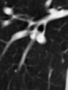
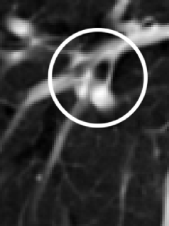
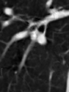
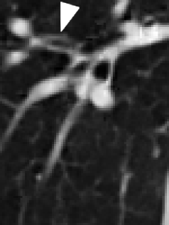
(a) original slice                (b) original transform         (c) mesh-based compensation   (d) block-based compensation

(blurred)                          (sharp)                              (more details)

Fig. 2: Zoom in one slice of the lowpass band of thorax2 for visual comparison, from left to right: (a) original corresponding slice, (b) original wavelet transform without compensation, (c) mesh-based compensation and (d) block-based compensation with filling. The blur of the original uncompensated transform can be seen especially in the marked circle. The block-based compensation method is able to conserve more details as can be seen in the area marked with an arrow in the right image.

the lowpass band and the corresponding original slices. For the original transform without a compensation method, the MSE computes to

$$\text{MSE}\left(\text{LP}_{\text{zero}},f\right)=\frac{1}{MNK}\sum_{m,n,k}\left|\text{LP}_{\text{zero},k}\left[m,n\right]-f_{2k}\left[m,n\right]\right|^{2}.$$ (6)

The computation of the $\text{MSE}\left(\text{LP}_{\text{block}},f\right)$ for the block-based displacement compensation, $\text{MSE}\left(\text{LP}_{\text{block+fill}},f\right)$ for the block-based displacement compensation with interpolation of the motion vector field and the $\text{MSE}\left(\text{LP}_{\text{mesh}},f\right)$ for mesh-based displacement compensation method is analogous.

For computing the peak signal to noise ratio (PSNR), the MSE is computed relative to the maximum intensity value $I_{\text{max}}$. The PSNR for the whole lowpass band of the original transform without compensation computes to

$$\text{PSNR}\left(\text{LP}_{\text{zero}},f\right)=10\log_{10}\left(\frac{I_{\text{max}}^{2}}{\text{MSE}\left(\text{LP}_{\text{zero}},f\right)}\right)\>\text{ [dB]}.$$ (7)

For a more exact analysis, the PSNR is also computed per slice. As different input data can have a different bit depth and thus a different maximum intensity, a direct comparison of the PSNR values is difficult. Subtracting two PSNR values results in a metric that gives the change of the MSE in dB. This results in the lowpass gain

$$G_{\text{LP},\text{MSE}} = \text{PSNR}\left(\text{LP}_{\text{dcm}},f\right)-\text{PSNR}\left(\text{LP}_{\text{zero}},f\right)$$

$$= 10\log_{10}\left(\frac{\text{MSE}\left(\text{LP}_{\text{zero}},f\right)}{\text{MSE}\left(\text{LP}_{\text{dcm}},f\right)}\right)\>\text{ [dB}]$$

that gives the gain in reduction of the MSE relative to the original transform in dB.

With the $\text{L}_{\infty}$-norm, the second metric calculates the maximum absolute distance between the lowpass band $\text{LP}_{i}$ and the corresponding original frames $f_{2i}$. While the MSE is an averaging metric the maximum absolute distance which is also desirable to be low. For the original transform it computes to

$$\text{L}_{\infty}\left(\text{LP}_{\text{zero}},f\right)=\underset{\forall m,n,k}{\max}\left|\text{LP}_{\text{zero},k}\left[m,n\right]-f_{2k}\left[m,n\right]\right|.$$ (9)

The computation for ‘block’, ‘block+fill’ and ‘mesh’ is again analogous.

3 Results

In our simulation we perform one wavelet decomposition step with and without displacement compensation and compare the characteristics of the resulting wavelet coefficients. We used a head and two thorax 3-D CT data sets. The CT data sets have a resolution of 512x512 with 32 slices (head), 65 slices (thorax1) and 67 slices (thorax2) and a bit depth of 12 bit per voxel. For comparison with video data we took details from the HEVC test sequences in class A, namely from the sequences people and traffic with a resolution of 512x512 pixels, all 150 frames. The CT data sets have an intensity component only so we used the luminance component of the video sequences that has a bit depth of 8 bit per pixel.

We used the implementation of the displacement compensation methods in the QccPack library [9]. As the library is available in C, we implemented the method for filling the unconnected pixels [10] in C as well. For the block-based compensation method we used a block size of 8x8 pixels and a search range of 8 pixels. For the mesh-based method we also used a grid size of 8 pixels. The blocks for the motion search have a size of 7x7 pixels and the search range was set to 8 pixels. As our main intention was to examine the properties of the extension of the wavelet transform for medical volume data, we did not optimize our code for speed so far. The complexity of the displacement estimation is comparable for the block-based and the mesh-based approach as the movement of the vertices is determined by block-matching. But the compensation step is a lot more complex for the mesh-based method as an interpolation is needed for the values in the deformed mesh.

	subband transform coding gain $G_{\text{SUB},\text{dcm}}$
	zero	mesh	block	block+fill
people	3.31	6.44	9.98

traffic 4.12 10.17 11.49 11.48

thorax1 5.45 7.96 13.08 13.08

thorax2 6.21 9.19 14.27 14.26

head 5.52 6.45 8.5 8.49

Table 1: Subband coding gain, ‘dcm’ is a placeholder for the displacement compensation methods the row below

& 38.01 46.39 47.19 46.56 8.38 9.18 8.55 62 68 60 60

thorax1 44.01 47.59 52.71 50.27 3.58 8.7 6.26 378 567 318 339

thorax2 44.75 48.76 53.65 51.21 4.01 8.9 6.46 490 437 354 357

head 43.27 43.74 46.56 44.84 0.47 3.29 1.57 502 1006 754 754

Table 2: Lowpass band results, PSNR on the left, $G_{\text{LP},\text{MSE}}$ in the middle, and $\text{L}_{\infty}\left(\text{LP}_{\text{dcm}},f\right)$ on the right. ‘dcm’ is a placeholder for the displacement compensation methods the row below

We perform a single wavelet decomposition step and then compare the characteristics of the highpass and the lowpass coefficients. For the video sequences the transform is performed along the time axis and for the CT volumes along the slice axis. The simulation results are summarized in Table 3 and Table 3. More detailed results are shown in Figure 3 where the metrics are evaluated and plotted per slice for the video sequence people and the medical CT volume thorax2.

For visual comparison of the lowpass bands of the different approaches, a zoom into one slice of the lowpass band of thorax2 is shown in Figure 2. Compared to the corresponding original slice in Figure 2 (a) the blurriness of the lowpass band of the original transform can be seen in Figure 2 (b). The lowpass bands of the compensated transforms in Figure 2 (c) and (d) represent the structures sharper and more detailed.

For the quantitative measures we first compare the subband transform coding gain reduction gain $G_{\text{SUB},\text{dcm}}$. The results are listed in Table 3. The interpolation of the motion vector field (‘block+fill’) has only minor influence on $G_{\text{SUB},\text{dcm}}$. For all examined data, the compensation methods lead to a significant increase of the subband transform coding gain and thus improve the energy compaction of the wavelet transform. Further, the block-based method is more capable of improving the transform for both kinds of data. For both thorax CT data sets, the transform gain can be improved by more than a factor of 2.

Second we compare the similarity of the lowpass band and the corresponding original slices. The first columns of Table 3 contain the lowpass $\text{PSNR}\left(\text{LP}_{\text{dcm}},f\right)$ in dB. The PSNR results suggest, that a compensation method is advantageous for all examined data. The gain of the compensation methods relative to the original transforms without compensation is listed in the columns entitled by lowpass gain $G_{\text{LP},\text{MSE}}$ in dB. For both kinds of data, the lowpass bands are more similar to the original slices for a compensated wavelet transform. While the gains for the CT volume head are lower, the gains for the displacement compensated transform of the thorax volumes are comparable to the gains for the MCTF of the video sequences. The interpolation of the motion vector field leads to a lower gain in MSE reduction but still higher than for the mesh-based method. The more detailed slice-wise results in Figure 3 (a) show a very similar behavior of the compensation methods for the video sequence people compared to the results in Figure 3 (c) for the CT volume thorax2.

(a) (b)

Legend:      \psfragscanon\psfrag{m30}{zero}\psfrag{m61}{block}\psfrag{m60}{block+fill}\psfrag{m100}{mesh}\psfrag{m110}{weinlich}\psfrag{m121}{block+den}\psfrag{m120}{block+fill+den}\includegraphics[width=405.16878pt]{img/legend-short}

(c) (d)

Fig. 3: Detailed results for the sequence people in the first row (a), (b) and for the medical CT volume thorax2 in the second row (c), (d). First column: PSNR of the lowpass band and the corresponding original slices, second column: the $\text{L}_{\infty}$-norm per slice of the lowpass band and the corresponding original slices. The placeholder ‘dcm’ stands for the displacement compensation method.

Third we compare the $\text{L}_{\infty}$-norm of the lowpass band and the corresponding original slices. The higher values for the medical CT volumes can be explained by the different bit depth. For all examined data, the $\text{L}_{\infty}$-norm for the mesh-based method is higher than for the block-based method. That means that the block-based method can model the occurring displacement better. For the video sequences the $\text{L}_{\infty}$-norm can be reduced by incorporating either of the two compensation methods while the block-based method leads to smaller values. For the CT volume head the maximum absolute distances are significantly higher for the coefficients resulting from the displacement compensated transform. That shows that the examined methods are not suitable to compensate the displacement in all kinds of medical CT volumes in general and, e.g., for the CT volume head a proper displacement compensation method needs to be found. For the two thorax CT volumes the results of the block-based method are similar to the video sequences though the reduction is smaller. The more detailed results in Figure 3 (b) and (d) also show a similar behavior for the medical CT volume thorax2.

4 Conclusion

For all examined types of data, the introduction of a displacement compensation step into the lifting structure leads to an increase of the transform coding gain by more than a factor of 2 and thus a better energy compaction for video data and thorax CT volumes. In our simulations the block-based displacement compensation performed better than the mesh-based method.

Further, we could show that a displacement compensation step can improve the similarity of the lowpass band to the corresponding original also for medical thorax CT volumes by 8 dB in terms of PSNR. This enlarges the quality and thus the usability of the lowpass band as downscaled version of the original volume. A next step is to examine the extension of the wavelet transform by a compensation step along the time axis of dynamical medical volume data.

It is not clear whether the compensated lowpass coefficients can be used directly for diagnostic purposes. Nevertheless, a scalable representation is advantageous for faster and more efficient browsing in a huge data volume. This can be very advantageous, e.g., in telemedicine.

Further work aims at a more detailed complexity analysis and an improvement of the inversion of the block-based compensation.

Acknowledgment

We gratefully acknowledge that this work has been supported by the Deutsche Forschungsgemeinschaft (DFG) under contract number KA 926/4-1.

References

- [1] A.R. Calderbank, I. Daubechies, W. Sweldens, and B.-L. Yeo, “Lossless Image Compression Using Integer to Integer Wavelet Transforms,” in Proc. Int. Conf. on Image Processing (ICIP), Washington, DC, USA, Oct. 1997, pp. 596–599.
- [2] V. Sanchez, R. Abugharbieh, and P. Nasiopoulos, “3-D Scalable Medical Image Compression With Optimized Volume of Interest Coding,” IEEE Trans. on Medical Imaging, vol. 29, no. 10, pp. 1808–1820, Oct. 2010.
- [3] L. Zeng, C.P. Jansen, S. Marsch, M. Unser, and P.R. Hunziker, “Four-dimensional wavelet compression of arbitrarily sized echocardiographic data,” IEEE Trans. on Medical Imaging, vol. 21, no. 9, pp. 1179–1187, 2003.
- [4] H.G. Lalgudi, A. Bilgin, M.W. Marcellin, A. Tabesh, M.S. Nadar, and T.P. Trouard, “Four-dimensional compression of fMRI using JPEG 2000,” in Proc. of SPIE Medical Imaging, San Diego, California, USA, Feb. 2005, vol. 5747, pp. 1028–1037.
- [5] J.U. Garbas, B. Pesquet-Popescu, and A. Kaup, “Methods and Tools for Wavelet-Based Scalable Multiview Video Coding,” IEEE Trans. on Circuits and Systems for Video Technology, vol. 21, no. 2, pp. 113–126, Feb. 2011.
- [6] J.-R. Ohm, “Three-dimensional subband coding with motion compensation,” IEEE Trans. on Image Processing, vol. 3, no. 5, pp. 559–571, 1994.
- [7] V. Sanchez, P. Nasiopoulos, and R. Abugharbieh, “Lossless compression of 4D medical images using H. 264/AVC,” in Proc. IEEE Int. Conf. on Acoustics, Speech, and Signal Processing (ICASSP), Toulouse, France, May 2006, pp. 1116–1119.
- [8] U.-E. Martin and A. Kaup, “Analysis of Compression of 4D Volumetric Medical Image Datasets Using Multi-View (MVC) Video Coding Methods,” in Proc. of SPIE Optical Engineering + Applications, San Diego, CA, USA, Aug. 2008, vol. 7075, p. 707507.
- [9] J.E. Fowler, “QccPack: An Open-Source Software Library for Quantization, Compression, and Coding,” in Proc. Applications of Digital Image Processing XXIII, San Diego, CA, USA, Aug. 2000, vol. 4115, pp. 294–301.
- [10] N. Bozinovic, J. Konrad, W. Zhao, and C. Vazquez, “On the Importance of Motion Invertibility in MCTF/DWT Video Coding,” in Proc. IEEE Int. Conf. on Acoustics, Speech, and Signal Processing (ICASSP), Philadelphia, PA, USA, Mar. 2005, vol. 2, pp. 49–52.
- [11] P.P. Vaidyanathan, “Filter Banks with Maximum Coding Gain and Energy Compaction,” in Asilomar Conf. on Signals, Systems and Computers, Asilomar, CA, USA, Nov. 1995, vol. 1, pp. 36 –40.