Maximum Centre-Disjoint Mergeable Disks

Abstract

Given a set of disks on the plane, the goal of the problem studied in this paper is to choose a subset of these disks such that none of its members contains the centre of any other. Each disk not in this subset must be merged with one of its nearby disks that is, increasing the latter’s radius. We prove that this problem is NP-hard. We also present polynomial-time algorithms for the special case in which the centres of all disks are on a line.

Keywords: Merging disks, map labelling, rotating maps, NP-hardness, geometric independent set.

1 Introduction

A motivating example for the problem studied in this paper is the following about drawing text labels on a digital map that can be rotated: suppose there are a number of points on the map that represent map features. To each of these feature points a text label is assigned that describe the feature, like the name a junction. When the map is rotated by the user, these labels must remain horizontal for the sake of readability, and therefore, they are rotated in the reverse direction around their feature point. Labels are difficult to read if they overlap, and therefore, only a non-overlapping subset of the labels are drawn on the map. If a label cannot be drawn because it overlaps with other labels, the text of its label must be appended to a nearby label that is drawn. The goal is to draw the maximum number of labels on the map such that none of them overlap when rotating the map. This is demonstrated in Figure 1. Part (a) shows four feature points and their labels. Part (b) shows the map when it is rotated 45 degrees counterclockwise; instead of rotating the map, the labels are equivalently rotated 45 degrees clockwise. Obviously the two labels on the left side of the map overlap. Part (c) shows what happens when these labels are merged. The remaining three labels never overlap when the map is rotated.

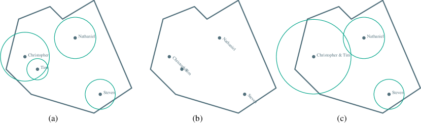
Figure 1: An example rotating map; (a) the initial configuration, (b) after rotating the map 45 degrees counterclockwise, (c) merging two of the labels.

Placing as many labels as possible on a map (known as map labelling) is a classical optimization problem in cartography and graph drawing [1]. For static maps, i.e. maps whose contents does not change, the problem of placing labels on a map can be stated as an instance of geometric independent set problem (sometimes also called packing for fixed geometric objects): given a set of geometric objects, the goal is to find its largest non-intersecting subset. In the weighted version, each object also has a weight and the goal is to find a non-intersecting subset of the maximum possible weight.

A geometric intersection graph, with a vertex for each object and an edge between intersecting objects, converts this geometric problem to the classical maximum independent set for graphs, which is NP-hard and difficult to approximate even within a factor of $n^{1-\epsilon}$, where $n$ is the number of vertices and $\epsilon$ is any non-zero positive constant [2]. Although the geometric version remains NP-hard even for unit disks [3], it is easier to approximate, and several polynomial-time approximation schemes (PTAS) have been presented for this problem [4, 5, 6, 7, 8].

Dynamic maps allow zooming, panning, or rotation, and labelling in such maps seems more challenging. Most work on labelling dynamic maps consider zooming and panning operations [10]. Gemsa et al. [11] were the first to formally study labelling rotating maps. With the goal of maximising the total duration in which labels are visible without intersecting other labels, they proved the problem to be NP-hard and presented a $1/4$-approximation algorithm and a PTAS, with the presence of restrictions on the distribution of labels on the map. Heuristic algorithms and Integer Linear Programming (ILP) formulations have also been presented for this problem [12, 13]. Note that in these problems, invisible labels do not get merged with visible labels. Yokosuka and Imai [14] examined a variant of this problem, in which all of the labels are always present in the solution and the goal is to maximise their size.

A related problem is crushing disks [15], in which a set of prioritized disks are given as input, whose radii grow over time, as map labels do when zooming in. When two disks touch, the one with the lower priority disappears. The radii of the disks grow linearly, and when a disk disappears, the radius of the other disk does not change. The goal is to find the order in which disks disappear and the process finishes when only one disk remains.

In this paper, we investigate a problem similar to geometric independent set for a set of disks, except that i) the disks in the output must be centre-disjoint (none of them can contain the centre of another) but they may overlap, ii) each disk that does not appear in the output must be merged with a disk, containing its centre, that does. When a disk is merged with another, the radius of the latter is increased by the radius of the former. Also to preserve the locality of the merges, a disk $A$ can be merged with another disk $B$, only if all disks closer to $B$ than $A$ (considering the distance between disk centres) are also merged with $B$, and after merging these closer disks, $B$ must contain the centre of $A$ (without this restriction, we presented a PTAS in an earlier paper [9]). This problem is formally defined in Section 2.

To observe how the introductory example at the beginning of this section reduces to this problem, consider the disks in Figure 1-(a). The disk centred at each feature point shows the region covered by its label during rotation. Only if a disk contains the centre of another, their corresponding labels intersect at some point during rotation. As another application of this problem, centre-disjoint disks can show the distribution of facilities in an area. For instance, Figure 2 shows the distribution of schools in Munich. It was obtained by placing a disk of radius 50 meters on each school (the coordinates of schools were obtained from OpenStreetMap data). Then, an integer program was used to obtain the maximum number of centre-disjoint disks in our problem (based on Definition 2.4).

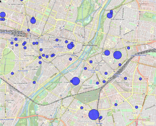
Figure 2: The distribution of schools in Munich; disks corresponding to neighbouring schools were merged to obtain larger, centre-disjoint disks.

We prove this problem to be NP-hard via a reduction from Planar Monotone 3-SAT [16]. Note that the centre-disjointness property of disks are used in the definition of transmission graphs of a set of disks, in which a vertex is assigned to each disk and a directed edge from a disk to another shows that the former contains the centre of the latter [17]. These graphs have been studied for interesting properties or their recognition [18, 17, 19], but those results do not apply to our problem.

We also study the problem when the centres of input disks are on a line. Many difficult problem become less challenging with this restriction. For instance, Biniaz et al. [20] study three problems about a set of points and disks on a line. For our problem, we present a polynomial-time algorithm that incrementally obtains a set of centre-disjoint disks with the maximum size.

This paper is organised as follows. In Section 2 we introduce the notation used in this paper and formally state the problem. Then, in Section 3 we show that the problem studied in this paper is NP-hard. In Section 4, we present a polynomial-time algorithm for the 1.5D variant of the problem, in which all disk centres are on a line. Finally, in Section 5 we conclude this paper.

2 Notation and Preliminary Results

Let $D=\{d_{1},d_{2},\dots,d_{n}\}$ be a set of $n$ disks. The radius of $d_{i}$ is denoted as $r_{i}$ and sometimes as $r_{d_{i}}$, and its centre is denoted as $p_{i}$.

Definition 2.1.

A function $\phi$ from $D$ to itself is an assignment, if $\phi(\phi(d_{i}))$ is $\phi(d_{i})$ for every $d_{i}$ in $D$. According to an assignment $\phi$, the disks in $D$ can be either selected or merged: if $\phi(d_{i})$ is $d_{i}$, the disk $d_{i}$ is selected, and otherwise, it is merged. The cardinality of an assignment, denoted as $\left|\phi\right|$, is the number of selected disks in $\phi$.

The relation defined by assignments (Definition 2.1) describes disk merges in our problem. For any disk $d_{i}$, if we have $\phi(d_{i})=d_{j}$ and $i\neq j$, it implies that $d_{i}$ is merged with $d_{j}$. On the other hand, the relation $\phi(d_{i})=d_{i}$ implies that it is a selected disk (is not merged with any other disk). Since a disk can be merged with selected disks only, for any disk $d_{i}$, we have $\phi(\phi(d_{i}))=\phi(d_{i})$.

Definition 2.2.

The aggregate radius of a selected disk $d_{i}$ with respect to assignment $\phi$, denoted with some misuse of notation as $r_{i}(\phi)$, is the sum of its radius and that of every disk merged with it, or equivalently,

$$r_{i}(\phi)=\sum_{\phi(d_{j})=d_{i}}r_{j}.$$

Let $\delta_{i}$ be the sequence of disks in $D\setminus\{d_{i}\}$, ordered increasingly by the distance of their centres from the centre of $d_{i}$, and let $\delta_{i}(j)$ denote its $j$-th disk. The $j$-th aggregate radius of $d_{i}$, denoted as $r_{i}(j)$, is defined as its aggregate radius if $\{\delta_{i}(1),\delta_{i}(2),\dots,\delta_{i}(j)\}$ are merged with $d_{i}$.

We can now define proper assignments (Definition 2.3). In the rest of this paper, the distance between two disks is defined as the Euclidean distance between their centres.

Definition 2.3.

An assignment $\phi$ is proper if it meets the following conditions.

1. The disk $\delta_{i}(j)$ can be merged with $d_{i}$, only if $\delta_{i}(k)$, for every $k$ where $1\leq k<j$, are also merged with $d_{i}$. In other words, all disks closer to $d_{i}$ than $\delta_{i}(j)$ are also merged with $d_{i}$.

2. The disk $\delta_{i}(j)$ can be merged with $d_{i}$, only if the distance between the centre of $d_{i}$ and $\delta_{i}(j)$ is less than $r_{i}(j-1)$. In other words, after merging $\delta_{i}(k)$ for $1\leq k<j$, $d_{i}$ must contain the centre of $\delta_{i}(j)$.

3. Selected disks must be centre-disjoint with respect to their aggregate radii; i.e. none of them can contain the centre of any other selected disk. More precisely, for indices $i$ and $j$ such that $i\neq j$, $\phi(d_{i})=d_{i}$, and $\phi(d_{j})=d_{j}$, we have $\left|p_{i}p_{j}\right|\geq r_{i}(\phi)+r_{j}(\phi)$.

Note the first two items in Definition 2.3 ensure the locality of the merges, which is especially important in the labeling application mentioned in the Introduction.

Definition 2.4.

Given a set of disks, in the Maximum Centre-Disjoint Mergeable Disks Problem (MCMD), the goal is to find a proper assignment of the maximum possible cardinality.

Figure 3 shows a configuration of five disks with more than one proper assignment. Disk $d_{3}$ can be merged with $d_{1}$, after which, $d_{1}$ would contain the centre of $d_{4}$ and $d_{5}$, both of which then have to be merged with $d_{1}$. These merges result in $d_{1}$ containing the centre of $d_{2}$, which would also be merged. Therefore, in this assignment $\phi_{1}$, we have $\phi_{1}(d_{i})=d_{1}$, for $1\leq i\leq 5$, and its cardinality is one. Alternatively, in assignment $\phi_{2}$ we can merge $d_{3}$ with $d_{2}$, as the latter contains the centre of the former. The remaining disks are centre-disjoint. Therefore, we have $\phi_{2}(d_{1})=d_{1}$, $\phi_{2}(d_{2})=d_{2}$, $\phi_{2}(d_{3})=d_{2}$, $\phi_{2}(d_{4})=d_{4}$, $\phi_{2}(d_{5})=d_{5}$, and its cardinality is four. Assignment $\phi_{2}$ maximises the number of selected disks, and is a solution to MCMD for the configuration of disks in Figure 3.

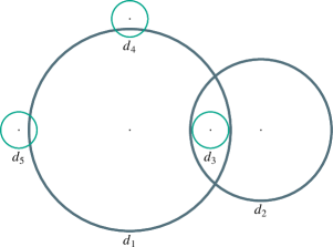
Figure 3: An example set of disks with more than one proper assignments.

Not every set of disks has a proper assignment. Figure 4 shows an example. Disk $d_{3}$ can be merged with either $d_{1}$ or $d_{2}$. If $d_{3}$ is merged with $d_{1}$, $d_{5}$ cannot be merged with $d_{2}$, because of the second condition of proper assignments: $d_{5}$ can be merged with $d_{2}$, only if all closer disks to $d_{2}$ are merged with it (but $d_{3}$ which is closer to $d_{2}$ than $d_{5}$ is not). Therefore, $d_{5}$ can be neither merged, nor selected (because its centre is contained in $d_{2}$). Similarly, if $d_{3}$ is merged with $d_{2}$, $d_{4}$ can neither be merged nor selected. Thus, there exists no proper assignment for these set of disks. In Section 3.2 we introduce a variant of MCMD by relaxing the second condition of Definition 2.3, in which every instance has a solution.

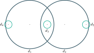
Figure 4: An example set of disks with no proper assignment.

3 Hardness of Maximum Centre-Disjoint Mergeable Disks

Instead of proving that the decision version of MCMD (Definition 3.1) is NP-complete, we show that even deciding whether a set of disks has a proper assignment (Definition 3.2) is NP-complete (clearly the latter implies the former). To do so, we perform a reduction from the NP-complete Planar Monotone 3-SAT (Definition 3.3) [21] to Proper MCMD (Definition 3.2).

3.1 Hardness of MCMD

Definition 3.1.

In the $k$-MCMD problem, we are given a set of disks and we have to decide if there exists a proper assignment of cardinality at least $k$ or not.

Definition 3.2.

In the Proper MCMD problem, we are given a set of disks and we have to decide if there exists a proper assignment.

Definition 3.3.

Monotone 3-SAT is a variant of 3-SAT, in which all variables of each clause are either positive or negative. An instance of Monotone 3-SAT is called Planar, if it can be modeled as a planar bipartite graph with parts $V$ corresponding to variables and $C$ corresponding to clauses; each vertex in $C$ is incident to at most three variables, which correspond to the variables that appear in the clause. Deciding if an instance of Planar Monotone 3-SAT is satisfiable is NP-complete [16].

It can be proved that every instance of Planar Monotone 3-SAT has a monotone rectilinear representation (Definition 3.4), and also, if for every instance of Planar Monotone 3-SAT its monotone rectilinear representation is also given, the problem remains NP-Complete [16].

Definition 3.4.

A monotone rectilinear representation of an instance of Planar Monotone 3-SAT is a drawing of the instance with the following properties: i) Variable are drawn as disjoint horizontal segments on the $x$-axis, ii) positive clauses are drawn as horizontal segments above the $x$-axis, iii) negative clauses are drawn as horizontal segments below the $x$-axis, iv) an edge is drawn as a vertical segment between a clause segment and the segments corresponding to its variable, and v) the drawing is crossing-free.

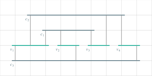
Figure 5: A monotone rectilinear representation of a Planar Monotone 3-SAT instance with three clauses and four variables.

Figure 5 shows a monotone rectilinear representation of an instance of Planar Monotone 3-SAT with three clauses, in which $c_{1}=v_{1}\lor v_{2}\lor v_{3}$, $c_{2}=v_{1}\lor v_{2}\lor v_{3}$, and $c_{3}=\neg v_{1}\lor\neg v_{2}\lor\neg v_{4}$.

Lemma 3.5.

For an instance of Planar Monotone 3-SAT with $v$ variables and $c$ clauses, there exists a monotone rectilinear representation on a two-dimensional integer grid with $c+1$ rows and $3c+v$ columns, such that horizontal segments, which represent variables and clauses, appear on horizontal grid lines, and vertical segments appear on vertical grid lines.

Proof.

Let $R$ be a monotone rectilinear representation of a Planar Monotone 3-SAT instance (such a representation certainly exists [16]). By extending horizontal segments of $R$ we get at most $c+1$ lines: one for the variables (the $x$-axis) and at most $c$ for clauses. Let $\ell_{1},\ell_{2},\dots,\ell_{m}$ be the lines that appear above the $x$-axis ordered by their $y$-coordinates. We move them (together with the segments appearing on them) so that, $\ell_{i}$ is moved to $y=i$; vertical segments that connect them to a segment on the $x$-axis may need to be shortend or lengthened during the movement. Given that the $x$-coordinate of the end points of horizontal segments, and also the vertical order of the segments, do not change, no new intersection is introduced by this transformation. The same is done for the lines that appear below the $x$-axis.

Repeating the same process for vertical segments, we get at most $3c$ vertical lines. We can similarly move these lines and the segments on them horizontally so that they appear in order and consecutively on vertical integer grid lines. Variables that do not appear in any clause, can be placed in at most $v$ additional vertical grid lines. This results in a $(c+1)\times(3c+v)$ grid. ∎

In the proof of Theorem 3.6, we create an instance of Proper MCMD from the monotone rectilinear representation an instance of Planar Monotone 3-SAT. In our construction, we use two types of disks:

• Normal disks, which by our construction, are always selected (their centres can never be inside any other disk). We call them sdisks for brevity.

• Disks of very small radius, which are contained in at least one sdisk, and thus, are surely merged in our construction. We call these disks mdisks. We assume that the radius of mdisks is so small compared to the radius of sdisks that after merging any number of mdisks with an sdisk, the centre of no new disk would enter the sdisk in our configuration. In the instance of Proper MCMD that we construct, each sdisk contains at least one mdisk.

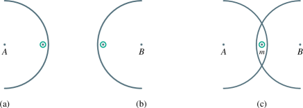
Figure 6: Two gadgets, joined at one of their mdisks.

We create a configuration of disks using gadgets, each of which consists of some mdisks and sdisks. The mdisks of a gadget are either internal (internal mdisks) or can be shared with other gadgets (shared mdisks). Parts (a) and (b) of Figure 6 show two gadgets (from each gadget, only an sdisk and an mdisk is shown). In Figure 6-(c) these two gadgets are joined at mdisk $m$. In a proper assignment, $m$ is merged either with an sdisk of $A$ or with an sdisk of $B$. With respect to gadget $A$, if $m$ is merged with $A$ in a proper assignment, we say that it is merged in, and otherwise, merged out.

We use the following gadgets in our construction. The gadgets and the distance between shared mdisks of each of them are shown in Figure 7; sdisks (denoted as $s_{i}$) are large disks and mdisks (denoted as $m_{i}$) are small disks (shared mdisks are distinguished with a darker colour).

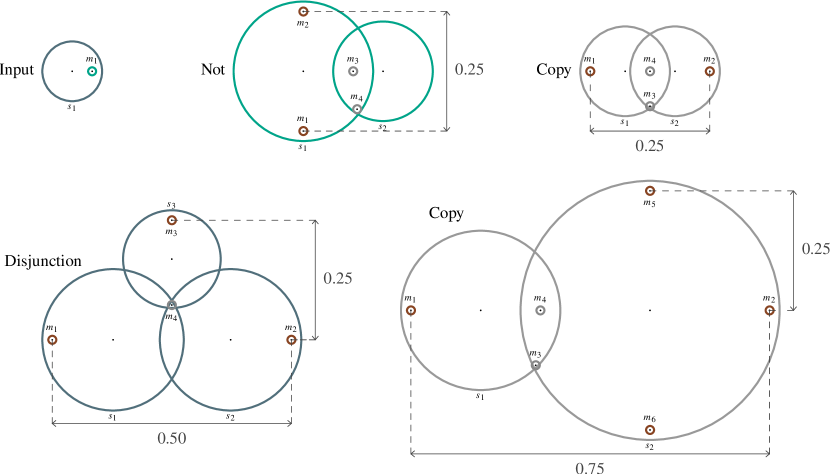
Figure 7: Gadgets used in the proof of Theorem 3.6.

• Input: It has only one shared mdisk, which can be either merged in or merged out.

• Copy: We use two gadgets for copy in our construction: one with two mdisks and one with four (both of them are demonstrated in Figure 7). The logic behind both of them is similar and is explained thus. If $m_{1}$ is merged in, $m_{2}$ (also $m_{5}$ and $m_{6}$ if present) is merged out, and if $m_{1}$ is merged out, $m_{2}$ (also $m_{5}$ and $m_{6}$) is merged in. To see why, note that $m_{3}$ can be merged either with $s_{1}$ or with $s_{2}$. If $m_{3}$ is merged with $s_{1}$, both $m_{1}$ and $m_{4}$ must also be merged with $s_{1}$, because $m_{3}$ is farther than both to $s_{1}$. Since $m_{4}$ is merged with $s_{1}$, $m_{2}$ (also $m_{5}$ and $m_{6}$) cannot be merged with $s_{2}$ and therefore they must be merged out. Similarly, if $m_{3}$ is merged with $s_{2}$, $m_{2}$ (also $m_{5}$ and $m_{6}$) must be merged with $s_{2}$ as well, and $m_{1}$ must be merged out.

• Disjunction: One or more of its shared mdisks are merged in. Clearly, $m_{4}$ must be merged with $s_{1}$, $s_{2}$, or $s_{3}$. If it is merged with $s_{i}$ ($i\in\{1,2,3\}$), $m_{i}$ must also be merged with $s_{i}$, and $m_{j}$ ($j\neq i$) may or may not be merged in.

• Not: Either both $m_{1}$ and $m_{2}$ are merge in or both of them are merged out. This is because $m_{4}$ can be merged either with $s_{1}$ or $s_{2}$. If it is merged with $s_{1}$, mdisks $m_{1}$, $m_{2}$, and $m_{3}$ must also be merged with $s_{1}$, because $m_{4}$ is farther than all of them. Otherwise, if $m_{4}$ is merged with $s_{2}$, mdisk $m_{3}$ must also be merged with $s_{2}$ and therefore, none of $m_{1}$ and $m_{2}$ can be merged with $s_{1}$, because $m_{3}$ (which is closer than both) is not merged with $s_{1}$. Thus, $m_{1}$ and $m_{2}$ must merge out.

Note that in 6-mdisk version of Copy gadget, one or two of its mdisks may not be shared with any other gadgets. If so, these mdisks must be removed from this instance of Copy.

Theorem 3.6.

Proper MCMD is NP-complete.

Proof.

It is trivial to show that Proper MCMD is in NP. To show that it is NP-hard, we reduce Planar Monotone 3-SAT to Proper MCMD. Let $I$ be an instance of Planar Monotone 3-SAT, with variables $V$ and clauses $C$. Based on Lemma 3.5, there exists a monotone rectilinear representation of $I$ on a $(\left|C\right|+1)\times(3\cdot\left|C\right|+\left|V\right|)$ integer grid. Let $R$ denote this representation.

We create an instance of Proper MCMD from $R$ as follows. The transformation is demonstrated in Figure 8, which corresponds to the monotone rectilinear representation of Figure 5.

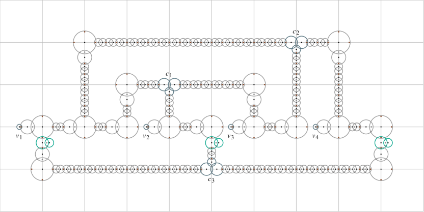
Figure 8: A Proper MCMD instance obtained from the Planar Monotone 3-SAT instance of Figure 5.

1. We replace the segment corresponding to a variable in $R$ with an Input gadget and a series of Copy gadgets. For each intersection of this segment with a vertical segment, a 6-mdisk Copy gadget is used.

2. Let $s$ be a horizontal segment corresponding to a clause in $R$. Three variables appear in the clause, for each of which there is a vertical segment that connects $s$ to a variable segment. For the first and last intersections, 6-mdisk Copy gadgets are used. For the 2nd intersection, we use a Disjunction gadget. These gadgets are connected using two chains of Copy gadgets.

3. For each vertical segment that connects a variable segment to a clause segment above the $x$-axis, we use a chain of Copy gadgets to connect the Copy gadget of the variable segment to the Copy or Disjunction gadget (if it is the 2nd intersection) of the clause segment. For segments that appear below the $x$-axis, we do likewise, except that we place a Not gadget before the chain of Copy gadgets.

Note that some of the gadgets of Figure 7 need to be rotated or mirrored. Also note that based on the sizes shown in Figure 7, shared mdisks always appear on grid lines in our construction. Given that the total area of the grid is bounded by $O(\left|C\right|^{2}\left|V\right|^{2})$, and on a segment of unit length, at most four gadgets can appear, the number of gadgets used in the resulting instance of Proper MCMD is at most $O(\left|C\right|^{2}\left|V\right|^{2})$. Thus, the size of the resulting Proper MCMD instance is polynomial in terms of the size of the input Planar Monotone 3-SAT instance.

Suppose there is a proper assignment for our Proper MCMD instance. We obtain an assignment $A$ of the variables of our Planar Monotone 3-SAT instance as follows. We assign one to a variable if the mdisk of its corresponding Input gadget is merged out, and assign zero otherwise. Consider any clause $c$ in our Planar Monotone 3-SAT instance. Let $g$ be the Disjunction gadget corresponding to $c$.

If $c$ is a positive clause, a chain of Copy gadgets connects the Input gadget of each of the variables that appear in $c$ to $g$. Therefore, if variable $v$ appears in the clause and if the shared mdisk of the Input gadget corresponding to $v$ is merged out, the mdisk of the last Copy gadget of its chain is merged in inside $g$. Since, one or more of the shared mdisks of $g$ are merged in, at least one of the terms in $g$ is satisfied. Similarly, if $c$ is a negative clause, because there is a Not gadget in the chain that connects each variable $v$ of $c$ to its Disjunction gadget, if the shared mdisk of the Input gadget corresponding to $v$ is merged out, the mdisk of the last Copy gadget of its chain is also merged out inside $g$. Since, one or more of the shared mdisks of $g$ are merged in, at least one of the variables in $g$ is not satisfied.

Therefore, the Planar Monotone 3-SAT instance is satisfied with assignment $A$.

For the reverse direction, suppose there exists an assignment $A$ of the variables, for which all clauses of $G$ are satisfied. We can obtain a proper assignment in our Proper MCMD instance as follows. For each variable $v$ in $V$, if $v$ is one, the shared mdisk of the Input gadget corresponding to $v$ is merged out, and otherwise, it is merged in. Let $c$ be a positive clause in which variable $v$ with value one appears (since $c$ is satisfied in $A$, variable $v$ must exist), and let $g$ be the gadget corresponding to clause $c$. Since $v$ is merged out, the mdisk of the last Copy gadget that connects the gadget corresponding to $v$ to $g$ is merged in with respect to $g$. This implies that one of the shared mdisks of the Disjunction gadget of each positive clause is merged in. We can similarly show that at least one of the shared mdisks of the Disjunction gadgets corresponding to negative caluses are also merged in. This yields a proper assignment for the Proper MCMD instance. ∎

In Corollary 3.7 we show that even if all disks have the same radius, the problem remains NP-hard.

Corollary 3.7.

Proper MCMD remains NP-complete, even if all disks are required to be of the same radius.

Proof.

We fix the radius of mdisks to $r=0.01$. We use the same construction as Theorem 3.6, with the difference that we replace each sdisk with a number of smaller disks of radius $r$ with the same centre, so that the sum of the radius of these smaller disks equals the radius of the sdisk. Since the disks added for each sdisk are not centre-disjoint, and their centre cannot be contained in some other disk, exactly one of them must be selected and after merging others, it reaches the size of the original sdisk. The rest of the proof of Theorem 3.6 applies without significant changes. ∎

3.2 Relaxing Merge Order

Due to the first condition of proper assignments (Definition 2.3), in a proper assignment $\phi$ of a set of disks $D$, a disk $d_{i}$ can be merged with another disk $d_{j}$, only if all closer disks to $d_{i}$ than $d_{j}$ are also merged with $d_{i}$. This condition, in addition to the second condition of Definition 2.3, ensures the locality of the merges. By requiring this ordering for merges, however, we get instances for which there is no solution, such as the one demonstrated in Figure 4. For such instances, a solution can be obtained by relaxing this condition. In this section, we relax the first condition of Definition 2.3.

Definition 3.8.

In an assignment $\phi$ for a set of disks $D$, let $\delta_{i}^{\phi}$ denote the sequence of disks assigned to selected disk $d_{i}$, ordered by their distance to $d_{i}$. Also, let $\delta_{i}^{\phi}(j)$ denote the $j$-th disk in this sequence.

Definition 3.9.

An assignment $\phi$ is uproper (short for unordered proper) if it meets the following conditions.

1. For each pair of possible indices $i$ and $j$, in which $\phi(d_{j})=d_{i}$, choose $k$ such that $\delta_{i}^{\phi}(k)=d_{j}$. The distance between $d_{i}$ and $d_{j}$ must be at most $r_{i}+\sum_{x=1}^{k-1}r_{\delta_{i}^{\phi}(x)}$. In other words, after merging all closer disks in $\delta_{i}^{\phi}$, $d_{i}$ must contain the centre of $d_{j}$.

2. Selected disks must be centre-disjoint with respect to their aggregate radii; i.e. none of them can contain the centre of any other selected disk.

Definition 3.10.

Given a set of disks, the goal in the Relaxed Maximum Centre-Disjoint Mergeable Disks Problem (RMCMD) is to find a uproper assignment of the maximum possible cardinality.

To show that RMCMD is NP-hard, in Theorem 3.11 we reduce the Partition problem to RMCMD. In Partition, we are given a set of positive integers and have to decide if there is a subset, whose sum is half of the sum of all numbers in the input list. Partition is known to be NP-complete.

Theorem 3.11.

RMCMD is NP-hard.

Proof.

We reduce Partition to RMCMD. Let $A=\{a_{1},a_{2},\dots,a_{n}\}$ be an instance of Partition and let $s$ be the sum of the members of $A$. Also let $e$ be any number smaller than one. We create an instance of RMCMD as follows.

1. Add disk $d_{1}$ of radius $2s$ and add $d_{2}$ with the same radius at distance $3s$ on the right of $d_{1}$.

2. Add $d_{3}$ at distance $5s/2+e$ above $d_{1}$ with radius $s$. Similarly, add $d_{4}$ at distance $5s/2+e$ above $d_{2}$ with the same radius.

3. Add one disk for each member of $A$ in the midpoint of $p_{1}$ and $p_{2}$, such that the radius of the one corresponding to $a_{i}$ is $a_{i}$.

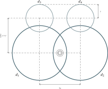
Figure 9: The construction in the proof of Theorem 3.11.

This is demonstrated in Figure 9. Let $\phi$ be the solution of this RMCMD instance. We show that there is a valid solution to the Partition instance if and only if the cardinality of $\phi$ is four.

Suppose $X$ is a subset of $A$ with sum $s/2$. We obtain an assignment from $X$ as follows: every disk corresponding to a member of $X$ is assigned to $d_{1}$ and others are assigned to $d_{2}$. Since the sum of the members of $X$ is $s/2$, the aggregate radii of both disks are exactly $5s/2$. Therefore, the centre of $d_{3}$ and $d_{4}$ are outside these disks. This yields a uproper assignment of cardinality 4.

For the reverse direction, suppose the cardinality of $\phi$ is four (note that it cannot be greater). If so, all of $d_{1}$, $d_{2}$, $d_{3}$, and $d_{4}$ are selected, and therefore, the aggregate radii of $d_{1}$ and $d_{2}$ are lower than $5s/2+e$. Given that the sum of the radii of the disks corresponding to members of $A$ is $s$, the sum of the set of disks assigned to $d_{1}$ and $d_{2}$ (and therefore the subsets of $A$ corresponding to them) are equal. ∎

4 Collinear Disk Centres

In this section we present a polynomial-time algorithm for solving MCMD for a set of disk with collinear centres. Note that even if disk centres are collinear, there may exist no proper assignments, as demonstrated in Figure 4. In the rest of this section, let $\lambda=\left<d_{1},d_{2},\dots,d_{n}\right>$ be a sequence of input disks $D$, ordered by the $x$-coordinate of their centres.

Definition 4.1.

Let $\phi$ be an assignment of $\{d_{1},d_{2},\dots,d_{n}\}$ and let $\phi^{\prime}$ be an assignment of $\{d_{1},d_{2},\dots,d_{x}\}$, such that $x\leq n$. $\phi$ is an extension of $\phi^{\prime}$, if for every disk $d_{i}$ in $\{d_{1},d_{2},\dots,d_{x}\}$, we have $\phi(d_{i})=\phi^{\prime}(d_{i})$. In other words, every selected disk in $\phi^{\prime}$ is also a selected disk in $\phi$, and every merged disk in $\phi^{\prime}$ is also merged with the same disk in $\phi$. Equivalently, when $\phi$ is limited to $\{d_{1},d_{2},\dots,d_{x}\}$, $\phi^{\prime}$ is obtained.

Definition 4.2.

$M(x,y,z)$ denotes the maximum cardinality of a proper assignment of $X=\{d_{1},d_{2},\dots,d_{x}\}$, such that the following conditions are met ($y\leq x\leq z\leq n$).

1. $d_{y}$ is its right-most selected disk.

2. $d_{y+1},d_{y+2},\dots,d_{x}$ are all merged with $d_{y}$.

3. $d_{z}$ is the right-most disk in $D$, where $z\geq x$, whose centre is contained in $d_{y}$ considering its aggregate radius.

Note that by the third condition of Definition 4.2, the centres of $d_{x+1},d_{x+2},\dots,d_{z}$ are inside $d_{y}$, but they are not merged with it, because they are outside $X$ and not present in the assignment which is limited to set $X$. Also, note that actually the second condition of Definition 4.2 is implied by its first condition: since $d_{y}$ is the right-most selected disk, all of the disks that appear on the right of $d_{y}$ in $X$ are surely merged. On the other hand, none of these disks can be merged with a selected disk $d_{w}$ on the left of $d_{y}$, because, in that case $d_{w}$ would contain the centre of $d_{y}$ and the assignment cannot be proper.

Theorem 4.3.

A proper assignment of the maximum cardinality for a set of $n$ disks $D$, in which the centres of all disks are collinear, can be computed in polynomial time.

Proof.

Let $M$ be defined as in Definition 4.2. Obviously, $\max_{i=1}^{n}M(n,i,n)$ is the cardinality of the solution to this MCMD instance.

The function $M$ accepts $O(n^{3})$ different input values. We can compute and store the value returned by $M$ in a three dimensional table, which we reference also as $M$. The values of the entries of $M$ are computed incrementally, as described in Algorithm 4.4. We explain the steps of this algorithm in what follows.

Algorithm 4.4.

Find a solution to MCMD for a set of collinear disks.

1. Compute the sequences $\delta_{i}$ for $1\leq i\leq n$ (Definition 2.2).

2. Initialize every entry of $M$ to $-\infty$.

3. For every possible value of $i$ from $1$ to $n$ and for every possible value of $j$ from $0$ to $n-1$ perform the following steps.

   1. Check to see if the first $j$ disks of $\delta_{i}$ can be merged with $d_{i}$, considering the conditions of Definition 2.3. If not, skip this iteration of this loop, and continue with the next iteration.

   2. Compute $A$, $a$, $b$, and $B$: $a$ and $b$ are the left-most and right-most disks in $\lambda$ that are merged with $d_{i}$, respectively. Also, $A$ and $B$ are the left-most and right-most disks of $D$ whose centres are contained in $d_{i}$, considering its aggregate radius.

   3. If $a=1$ and $M(b,i,B)<1$, assign 1 to $M(b,i,B)$.

   4. If $a>1$, for every possible value of $t$ from $1$ to $A-1$ and for every possible value of $k$ from $0$ to $n-2$ do as follows.

      1. Check if the first $k$ disks of $\delta_{t}$ can be merged with $d_{t}$ (based on Definition 2.3).

      2. Compute $f$ and $g$: $d_{f}$ is the right-most disk that is merged with $\delta_{t}$, and $d_{g}$ is the right-most disk of $D$ whose centre is contained in $d_{t}$, considering its aggregate radius.

      3. If $f\geq a$, $f\neq a-1$, or $g\geq i$ skip this value of $k$ ($\phi_{L}$ cannot be extended to obtain $\phi$).

      4. Replace the value of $M(b,i,B)$ with the maximum of its value and $M(a-1,t,g)+1$.

4. Compute and return $\max_{i=1}^{n}M(n,i,n)$.

Steps 1 and 2 of the algorithm initialize $M$ and $\delta_{i}$. In Step 3, we consider different cases in which $d_{i}$, for $1\leq i\leq n$ in order, is selected and update the value of different entries of $M$. For every possible value of $j$ from $0$ to $n-1$, suppose $j$ disks are merged with $d_{i}$. These disks are the first $j$ disks of $\delta_{i}$ by the first condition of Definition 2.3.

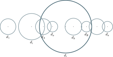
Figure 10: Demonstrating the symbols used in Theorem 4.3.

Let $S$ denote the set of such disks. If this is not possible (the centre of one of these disks is not contained in $d_{i}$, after merging its previous disks), we skip this value of $j$, because it fails the second condition of Definition 2.3 (Step 3.a). Note that if there exists no proper assignment in which $j$ disks are merged with $d_{i}$, a greater number of disks cannot be merged with $d_{i}$ in any assignment, and we can safely skip the remaining values of $j$ and continue the loop of Step 3 by incrementing the value of $i$.

Let $a$, $b$, $A$, and $B$ be defined as Step 3.b. If $a=1$, selecting $d_{i}$ and merging with it every disk in $\{d_{1},d_{2},\dots,d_{b}\}\setminus\{d_{i}\}$ is a proper assignment of the first $b$ disks of $\lambda$ with cardinality one. Therefore, we update the value of $M(b,i,B)$ to be at least one in step 3.c.

If $a>1$, let $\phi$ be any assignment of $\{d_{1},\dots,d_{b}\}$, in which i) $d_{i}$ is selected, ii) the members of $S$ are merged with $d_{i}$, and iii) the members of $\{d_{A},\dots,d_{a-1}\}\cup\{d_{b+1},\dots,d_{B}\}$ are contained in $d_{i}$ after merging the members of $S$ with $d_{i}$. By the definition of $M$, the value of $M(b,i,B)$ cannot be smaller than the cardinality of $\phi$. When $\phi$ is limited to $L=\{d_{1},\dots,d_{a-1}\}$, it specifies a proper assignment of $L$. We denote this assignment with $\phi_{L}$. We compute the value of $M(b,i,B)$ by considering all possible assignments for $\phi_{L}$ and extending them to obtain $\phi$ by selecting $d_{i}$.

Let $d_{t}$ be the right-most selected disk of $\phi_{L}$. This is demonstrated in Figure 10. The following conditions hold.

1. We have $t<A$, because $\{d_{A},\dots,d_{a-1}\}$ are contained in $d_{i}$ in $\phi$, and $d_{t}$ cannot be a selected disk if $t\geq A$. Therefore, disks $\{d_{t+1},\dots,d_{a-1}\}$ are merged with $d_{t}$ in $\phi_{L}$.

2. Suppose $k$ disks are merged with $d_{t}$ in $\phi_{L}$. Let $d_{f}$ be the right-most vertex of $D$ contained in $d_{t}$ after merging disks in $\phi_{L}$. We have $f<i$ (otherwise, $d_{f}$ would contain the centre of $d_{i}$, and $d_{i}$ cannot be selected in $\phi$). Also let $d_{g}$ be the right-most vertex of $D$ contained in $d_{f}$. We have $g<i$; otherwise, $d_{f}$ would contain the centre of $d_{i}$ and $\phi$ cannot be an extension of $\phi_{L}$.

By trying possible values of $t$ and $k$ that meet these conditions (Step 3.d), we find the maximum cardinality of $\phi_{L}$, which has been computed in the previous steps of this algorithm as $M(a-1,t,g)$. Since $\phi$ is an extension of $\phi_{L}$ by adding exactly one selected disk $d_{i}$, the maximum cardinality of $\phi$ therefore is at least $1+M(a-1,t,g)$. Thus, we have

$$M(b,i,B)\geq 1+\max_{\textit{$t$ and $k$, as above}}M(a-1,t,g)$$

Step 3.d.iv updates $M(b,i,B)$ to be at least this value. ∎

Theorem 4.5.

The time complexity of computing $M$ for a set of $n$ disks, as described in Theorem 4.3, is $O(n^{5})$.

Proof.

We analyse Algorithm 4.4. Constructing $\delta_{i}$ (step 1) can be done in $O(n^{2}\log n)$ and initializing $M$ (step 2) can be done in $O(n^{3})$. For each pair of values for $i$ and $j$, steps 3.a-c can be performed in $O(n)$. In step 3.d, $O(n^{2})$ possible cases for $t$ and $k$ are considered, and for each of these cases, the steps i, ii, iii, and iv can be performed in $O(n)$. Since the loop of step 3 is repeated $O(n^{2})$ times, the time complexity of the whole algorithm is $O(n^{5})$. ∎

5 Concluding Remarks

We introduced a variant of geometric independent set for a set of disks, such that the disks that do not appear in the output must be merged with a nearby disk that does (the problem was stated formally in Section 2). We proved that this problem is NP-hard (Theorem 3.6). Also by relaxing one of the conditions of the problem, we introduced a less restricted variant, which was proved NP-hard as well (Theorem 3.11). We presented a polynomial-time algorithm for the case in which disk centres are collinear.

Several interesting problems call for further investigation, such as: i) general approximation algorithms, ii) studying the case in which the number of disks that can be merged with a selected disk is bounded by some constant, and iii) solving MCMD when disks are pierced by a line.

References

- [1] Formann, M. and Wagner, F. (1991) A packing problem with applications to lettering of maps. Symposium on Computational Geometry (SoCG), North Conway, NH, USA, 10-12 June, pp. 281–288. ACM.
- [2] Håstad, J. (1999) Clique is hard to approximate within . Acta Math., 182, 105–142.
- [3] Fowler, R. J., Paterson, M., and Tanimoto, S. L. (1981) Optimal packing and covering in the plane are NP-complete. Information Processing Letters, 12, 133–137.
- [4] Hochbaum, D. S. and Maass, W. (1985) Approximation schemes for covering and packing problems in image processing and VLSI. J. ACM, 32, 130–136.
- [5] Agarwal, P. K., van Kreveld, M. J., and Suri, S. (1998) Label placement by maximum independent set in rectangles. Comput. Geom., 11, 209–218.
- [6] Erlebach, T., Jansen, K., and Seidel, E. (2005) Polynomial-time approximation schemes for geometric intersection graphs. SIAM J. Comput., 34, 1302–1323.
- [7] Chan, T. M. (2003) Polynomial-time approximation schemes for packing and piercing fat objects. J. Algorithms, 46, 178–189.
- [8] Chan, T. M. and Har-Peled, S. (2012) Approximation algorithms for maximum independent set of pseudo-disks. Discrete & Comput. Geom., 48, 373–392.
- [9] Rudi, A. G. (2021) Maximizing the number of visible labels on a rotating map. Sci. Ann. Comput. Sci., 31, 275–287.
- [10] Been, K., Daiches, E., and Yap, C.-K. (2006) Dynamic map labeling. IEEE Trans. Vis. Comput. Graph., 12, 773–780.
- [11] Gemsa, A., Nöllenburg, M., and Rutter, I. (2011) Consistent labeling of rotating maps. Comput. Geom., 7, 308–331.
- [12] Gemsa, A., Nöllenburg, M., and Rutter, I. (2016) Evaluation of labeling strategies for rotating maps. ACM J. Experim. Algor., 21, 1.4:1–1.4:21.
- [13] Cano, R. G., de Souza, C. C., and de Rezende, P. J. (2017) Fast optimal labelings for rotating maps. Workshop on Algorithms and Computation (WALCOM), Hsinchu, Taiwan, 29-31 March, pp. 161–173. Springer.
- [14] Yokosuka, Y. and Imai, K. (2017) Polynomial time algorithms for label size maximization on rotating maps. J. Inform. Process., 25, 572–579.
- [15] Funke, S., Krumpe, F., and Storandt, S. (2016) Crushing disks efficiently. IWOCA, Helsinki, Finland, 17-19 August, pp. 43–54. Springer.
- [16] de Berg, M. and Khosravi, A. (2010) Optimal binary space partitions in the plane. COCOON, Nha Trang, Vietnam, 19-21 July, pp. 216–225. Springer.
- [17] Kaplan, H., Klost, K., Mulzer, W., Roditty, L., Seiferth, P., and Sharir, M. (2019) Triangles and girth in disk graphs and transmission graphs. European Symposium on Algorithms (ESA), Munic/Garching, Germany, 9-11 September, pp. 64:1–64:14. Schloss Dagstuhl - Leibniz-Zentrum für Informatik.
- [18] Kaplan, H., Mulzer, W., Roditty, L., and Seiferth, P. (2018) Spanners for directed transmission graphs. SIAM J. Comput., 47, 1585–1609.
- [19] Klost, K. and Mulzer, W. (2018) Recognizing generalized transmission graphs of line segments and circular sectors. LATIN, Buenos Aires, 16-19 April, pp. 683–696. Springer.
- [20] Biniaz, A., Bose, P., Carmi, P., Maheshwari, A., Munro, J. I., and Smid, M. H. M. (2018) Faster algorithms for some optimization problems on collinear points. Symposium on Computational Geometry (SoCG), Budapest, Hungary, 11-14 June, pp. 8:1–8:14. Schloss Dagstuhl - Leibniz-Zentrum für Informatik.
- [21] Lichtenstein, D. (1982) Planar formulae and their uses. SIAM J. Comput., 11, 329–343.