The Low-Redshift Lyman Continuum Survey:
Optically Thin and Thick Mg ii Lines as Probes of Lyman Continuum Escape

Abstract

The Mg ii $\lambda$$\lambda$2796, 2803 doublet has been suggested to be a useful indirect indicator for the escape of Ly$\alpha$ and Lyman continuum (LyC) photons in local star-forming galaxies. However, studies to date have focused on small samples of galaxies with strong Mg ii or strong LyC emission. Here we present the first study of Mg ii probing a large dynamic range of galaxy properties, using newly obtained high signal-to-noise, moderate-resolution spectra of Mg ii for a sample of 34 galaxies selected from the Low-redshift Lyman Continuum Survey. We show that the galaxies in our sample have Mg ii profiles ranging from strong emission to P-Cygni profiles, and to pure absorption. We find there is a significant trend (with a possibility of spurious correlations of $\sim$ 2%) that galaxies detected as strong LyC Emitters (LCEs) also show larger equivalent widths of Mg ii emission, and non-LCEs tend to show evidence of more scattering and absorption features in Mg ii. We then find Mg ii strongly correlates with Ly$\alpha$ in both equivalent width and escape fraction, regardless of whether the emission or absorption dominates the Mg ii profiles. Furthermore, we present that, for galaxies categorized as Mg ii emitters (MgE), one can adopt the information of Mg ii, metallicity, and dust to estimate the escape fraction of LyC within a factor of $\sim$ 3. These findings confirm that Mg ii lines can be used as a tool to select galaxies as LCEs and to serve as an indirect indicator for the escape of Ly$\alpha$ and LyC.

1 Introduction

In the last decades, considerable observational efforts have been directed towards studying the escape of Lyman continuum (LyC) photons from galaxies and attempting to explain the last phase transition of the universe, i.e., Cosmic Reionization. Various publications point out that star-forming (SF) galaxies can be responsible for the epoch of reionization (EoR). These include studies of low-redshift galaxies (z $\lesssim$ 1, e.g., Heckman et al. 2001; Bergvall et al. 2006; Leitet et al. 2013; Borthakur et al. 2014; Leitherer et al. 2016; Izotov et al. 2016a; b; Puschnig et al. 2017; Izotov et al. 2018a; b; Wang et al. 2019; 2021; Chisholm et al. 2020; Izotov et al. 2021; Chisholm et al. 2022; Flury et al. 2022a; b; Izotov et al. 2022; Marques-Chaves et al. 2022a; Saldana-Lopez et al. 2022; Xu et al. 2022), and moderate- to high-redshifted galaxies (z $\sim$ 2 – 4, e.g., Robertson et al. 2015; Vanzella et al. 2016; de Barros et al. 2016; Shapley et al. 2016; Bian et al. 2017; Marchi et al. 2017; 2018; Steidel et al. 2018; Vanzella et al. 2018; Fletcher et al. 2019; Rivera-Thorsen et al. 2019; Ji et al. 2020; Mestrić et al. 2020; Vielfaure et al. 2020; Naidu et al. 2022; Begley et al. 2022; Rivera-Thorsen et al. 2022; Marques-Chaves et al. 2022b). These galaxies are proposed to be analogs of high-redshift (z $\sim$ 6 – 8) ones at EoR (e.g., Schaerer et al. 2016; Boyett et al. 2022).

Due to the attenuation by Lyman limit systems (LLS) and/or neutral intergalactic medium (IGM), it is challenging to detect LyC at $z\gtrsim 5$ (Inoue et al. 2014; Worseck et al. 2014; Becker et al. 2021; Bosman et al. 2022). Therefore, various indirect indicators have been developed from lower redshift analogs (see a summary in Flury et al. 2022a; b). One of the leading indicators is the Ly$\alpha$ emission (e.g., Verhamme et al. 2015; Henry et al. 2015; Dijkstra et al. 2016; Verhamme et al. 2017; Jaskot et al. 2019; Gazagnes et al. 2020; Kakiichi & Gronke 2021; Izotov et al. 2022). Given the resonance nature of Ly$\alpha$, the escape of Ly$\alpha$ photons contains information about the neutral hydrogen in/around the galaxy, and leaves footprints on the Ly$\alpha$ emission line profiles (e.g., Izotov et al. 2018b; Gazagnes et al. 2020; Flury et al. 2022b; Le Reste et al. 2022). Nonetheless, since Ly$\alpha$ photons can be also absorbed by neutral IGM, the interpretation of Ly$\alpha$ profiles for high-z galaxies (z $\gtrsim$ 4) is non-trivial (e.g., Stark et al. 2011; Schenker et al. 2014; Gronke et al. 2021; Hayes et al. 2021).

The Mg ii $\lambda$$\lambda$2796, 2803 doublet has been commonly detected as a pair of absorption lines in galaxies, which trace the galactic outflows and their feedback effects (e.g., Weiner et al. 2009; Erb et al. 2012; Finley et al. 2017; Wang et al. 2022). However, recently, Mg ii has been found to show strong doublet emission lines in galaxies which are classified as Lyman continuum emitter (LCEs) candidates. Various publications suggest that the escape of Mg ii correlates with that of Ly$\alpha$ and LyC in SF galaxies (Henry et al. 2018; Chisholm et al. 2020; Naidu et al. 2022; Xu et al. 2022; Izotov et al. 2022; Seive et al. 2022).

Mg ii emission was studied by Henry et al. (2018) in a sample of 10 compact SF galaxies. By the first time, they showed that the escape of Mg ii correlates with the escape of Ly$\alpha$. This result is interpreted as evidence that both Mg ii and Ly$\alpha$ photons escape from the galaxies through a similar path of low column density gas. Indeed, Chisholm et al. (2020) point out that the flux ratios between the doublet lines of Mg ii [i.e., F(Mg ii 2796)/F(Mg ii 2803), hereafter, $R$] can be used to trace the column density of neutral hydrogen. They and Xu et al. (2022) combined the Mg ii emission, metallicity, and dust attenuation to predict f${}_{\text{esc}}^{\text{ LyC}}$, and found that the predicted f${}_{\text{esc}}^{\text{ LyC}}$ correlates with the observed f${}_{\text{esc}}^{\text{ LyC}}$ in samples of galaxies with strong Mg ii emission lines. Xu et al. (2022) also found that galaxies selected with strong Mg ii emission lines might be more likely to leak LyC than similar galaxies with weaker Mg ii. In an independent sample, Izotov et al. (2022) confirmed that escaping LyC emission is detected predominantly in galaxies with $R$ $\gtrsim$ 1.3, which indicates that optical depth of Mg ii is low (i.e., $\tau_{2803}$$\lesssim$ 0.5, Chisholm et al. 2020). Therefore, a high $R$ ratio can be used to select LCEs candidates.

Mg ii emission lines are also detected in higher redshift SF galaxies. For example, in the stacks of bright Ly$\alpha$ emitters (LAEs) at z $\sim$ 2, Naidu et al. (2022) found that LCE candidates tend to have $R$ close to 2, and the Mg ii emission is closer to the systemic velocity (instead of redshifted in non-LCEs). In addition, Witstok et al. (2021) found in a lensed z $\sim$ 5 galaxy, the escape of Mg ii photons is consistent with that of Ly$\alpha$. However, Katz et al. (2022) pointed out from the hydro-cosmological simulations that Mg ii is a useful diagnostic of f${}_{\text{esc}}^{\text{ LyC}}$ only in the optically thin regime.

Though all of these studies support the hypothesis that strong Mg ii emission lines and a high $R$ ratio can serve as a good indirect indicator for Ly$\alpha$ and LyC escape, there exist two caveats. (1) Existing samples are commonly small and only focused on SF galaxies with strong Mg ii emission lines and/or galaxies as strong LyC emitters. The latter also results in substantial Mg ii emission lines. Similar SF galaxies with Mg ii as weaker emission lines, P-Cygni profiles, or absorption lines have not been systematically studied in observations. (2) Some of these studies only have low signal-to-noise (S/N) Mg ii spectra (e.g., Naidu et al. 2022; Xu et al. 2022; Izotov et al. 2022). Their determinations of $R$, and the subsequent inference of Mg ii optical depth, have more scatter due to the low S/N spectra.

In this paper, we further study Mg ii as an indirect indicator for the escape of Ly$\alpha$ and LyC, while we attempt to mitigate the two caveats noted above. We focus on galaxies from Low-redshift Lyman Continuum Survey (LzLCS, Flury et al. 2022a), where a large sample of 66 LCEs candidates are selected without reference to their Mg ii emission lines. For 34 out of 66 LzLCS galaxies, we present ground-based follow-up spectroscopy of the Mg ii feature. These data provide higher spectral resolution and S/N than SDSS/BOSS, along with coverage of Mg ii in galaxies where it is blueward of the SDSS bandpass. As we will show, these data achieve more secure measurements of the Mg ii properties, ultimately validating the use of Mg ii as an indirect indicator for the escape of Ly$\alpha$ and LyC.

The structure of the paper is as follows. In Section 2,we introduce the observations, data reduction, and basic measurements of optical emission lines. In Section 3, we present how we derive various important parameters from the observed Mg ii doublet. We show the main results in Section 4, including the comparisons of Mg ii with Ly$\alpha$ and LyC. We conclude the paper in Section 5.

2 Observations, Data Reductions, and Basic Analyses

2.1 Ultraviolet Spectra for LyC and Ly$\alpha$ Regions

In this study, we focus on LCE candidates from the Low-redshift Lyman Continuum Survey (LzLCS, Flury et al. 2022a), which contains 66 SF galaxies at z $\sim$ 0.3. The survey obtained rest-frame ultraviolet (UV) spectra for each galaxy with the G140L grating on Hubble Space Telescope/Cosmic Origins Spectrograph (HST/COS) under program GO 15626 (PI: Jaskot). Both LyC and Ly$\alpha$ regions have been covered. The detailed data reductions of G140L data as well as the analysis of Ly$\alpha$ and LyC escape are presented in Flury et al. (2022a). In this paper, we adopt their derived quantities for LyC and Ly$\alpha$. These mainly include their escape fractions and the equivalent widths (EW) for Ly$\alpha$.

Table 1: Follow-up Observations and Basic Properties for Galaxies in Our Sample

ID	RA	Dec	$z^{1}$	Instrument2	Date3	Exp.3	SDSS-u4	$E(B-V)_{\text{MW}}^{5}$	$E(B-V)_{\text{int.}}^{6}$
					(mm/dd/yyyy)	(s)	(mag)
J0957+2357	09:57:00	+23:57:09	0.2444	MMT/Blue	04/08/2019	4800	18.42	0.0287	0.3007
J1314+1048	13:14:19	+10:47:39	0.2960	MMT/Blue	04/08/2019	3600	19.69	0.0371	0.1621
J1327+4218	13:26:33	+42:18:24	0.3176	MMT/Blue	04/08/2019	3600	20.48	0.0173	0.1641
J1346+1129	13:45:59	+11:28:48	0.2371	MMT/Blue	04/08/2019	3600	19.00	0.0231	0.2022
J1410+4345	14:10:13	+43:44:35	0.3557	MMT/Blue	04/08/2019	7200	21.70	0.0196	0.1413
J0926+3957	09:25:52	+39:57:14	0.3141	MMT/Blue	04/09/2019	7200	21.27	0.0270	0.1364
J1130+4935	11:29:33	+49:35:25	0.3448	MMT/Blue	04/09/2019	7200	21.50	0.0292	0.0446
J1133+4514	11:33:04	+65:13:41	0.2414	MMT/Blue	04/09/2019	7200	20.14	0.0158	0.0886
J1246+4449	12:46:19	+44:49:02	0.3220	MMT/Blue	04/09/2019	4800	20.48	0.0200	0.1595
J0723+4146	07:23:26	+41:46:08	0.2966	MMT/Blue	02/19/2020	7200	20.89	0.0467	0.0097
J0811+4141	08:11:12	+41:41:46	0.3329	MMT/Blue	02/19/2020	7200	21.17	0.0383	0.1150
J1235+0635	12:35:19	+06:35:56	0.3326	MMT/Blue	02/19/2020	6000	20.72	0.0333	0.0782
J0814+2114	08:14:09	+21:14:59	0.2271	MMT/Blue	02/20/2020	1800	18.91	0.0336	0.1800
J0912+5050	09:12:08	+50:50:09	0.3275	MMT/Blue	02/20/2020	9600	20.56	0.0245	0.1088
J1301+5104	13:01:28	+51:04:51	0.3476	MMT/Blue	02/20/2020	2500	20.04	0.0222	0.0974
J0047+0154	00:47:43	+01:54:40	0.3535	MMT/Blue	01/09/2021	3600	20.28	0.0312	0.1760
J0826+1820	08:26:52	+18:20:52	0.2972	MMT/Blue	01/09/2021	7200	21.35	0.0328	0.0300
J1158+3125	11:58:55	+31:25:59	0.2430	MMT/Blue	01/09/2021	2700	19.27	0.0226	0.1037
J1248+1234	12:48:35	+12:34:03	0.2635	MMT/Blue	01/09/2021	6900	20.16	0.0519	0.0627
J0113+0002	01:13:09	+00:02:23	0.3060	MMT/Blue	01/10/2021	7200	20.56	0.0312	$<$1E-4
J0129+1459	01:29:10	+14:59:35	0.2799	MMT/Blue	01/10/2021	4800	20.11	0.0688	0.0729
J0917+3152	09:17:03	+31:52:21	0.3003	MMT/Blue	01/10/2021	3300	19.78	0.0204	0.1920
J1033+6353	10:33:44	+63:53:17	0.3465	MMT/Blue	01/10/2021	2700	19.84	0.0160	0.0819
J1038+4527	10:38:16	+45:27:18	0.3256	MMT/Blue	01/10/2021	2700	19.40	0.0241	0.2506
J0036+0033	00:36:01	+00:33:07	0.3480	VLT/X-Shooter	11/05/2020	2800	21.83	0.0278	0.2007
J0047+0154	00:47:43	+01:54:40	0.3537	VLT/X-Shooter	10/23/2020	5500	20.28	0.0312	0.0699
J0113+0002	01:13:09	+00:02:23	0.3062	VLT/X-Shooter	10/23/2020	5500	20.56	0.0312	0.1144
J0122+0520	01:22:17	+05:20:44	0.3655	VLT/X-Shooter	10/23/2020	5500	21.38	0.0559	0.1166
J0814+2114	08:14:09	+21:14:59	0.2271	VLT/X-Shooter	12/21/2020	2800	18.91	0.0335	0.1984
J0911+1831	09:11:13	+18:31:08	0.2622	VLT/X-Shooter	01/16/2021	2800	19.79	0.0279	0.1106
J0958+2025	09:58:38	+20:25:08	0.3016	VLT/X-Shooter	02/04/2021	2800	19.86	0.0347	0.0650
J1310+2148	13:10:37	+21:48:17	0.2830	VLT/X-Shooter	04/10/2021	5500	20.40	0.0204	0.0924
J1235+0635	12:35:19	+06:35:56	0.3327	VLT/X-Shooter	01/12/2022	5500	20.72	0.0333	0.0782
J1244+0215	12:44:23	+02:15:40	0.2394	VLT/X-Shooter	03/08/2022	2800	19.56	0.0424	0.0673
J0834+4805	08:34:40	+48:05:41	0.3425	HET/LRS2	12/30/2021	5400	20.62	0.0383	0.1741
J0940+5932	09:40:01	+59:32:44	0.3716	HET/LRS2	01/24/2022	5400	20.80	0.0380	0.4158
J1517+3705	15:17:07	+37:05:12	0.3533	HET/LRS2	07/22/2022	6300	20.87	0.0411	0.0005
J1648+4957	16:48:49	+49:57:51	0.3818	HET/LRS2	05/27/2022	5400	21.93	0.0374	0.0070
Note. – (1)  Redshift of the objects derived from fitting the Balmer emission lines. (2)  Instruments that are used for the follow-up observations (Section 2.2). (3)  Observation start-date and exposure time in seconds, respectively. (4)  The u-band magnitudes from SDSS photometry. (5)  Milky Way dust extinction obtained from Galactic Dust Reddening and Extinction Map (Schlafly & Finkbeiner 2011) at NASA/IPAC Infrared Science Archive. (6)  The internal nebular dust extinction of the galaxy derived from Balmer lines (Section 2.3).

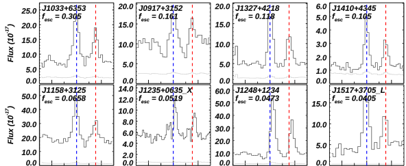
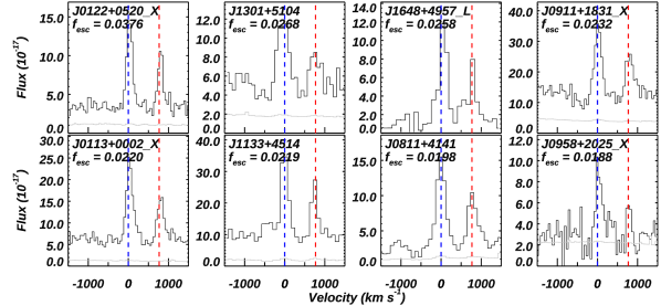
Figure 1: The final reduced Mg ii spectra for LzLCS galaxies in velocity space, with data taken from either MMT blue channel spectrograph or VLT/X-Shooter spectrograph. For X-Shooter and LRS2 observations, we mark them with an extra ‘X’ and ‘L’ at the end of object names, respectively. The y-axes are in units of 10^-17 ergs s^-1 cm^-2 Å^-1. The data and corresponding errors are shown in black and gray. Objects are ordered by measured f${}_{\text{esc}}^{\text{ LyC}}$ values published in Flury et al. (2022a), which are also shown in the top-left corner of each panel. The blue and red lines represent the position of $v$ = 0 km s^-1 for Mg ii $\lambda$2796 and 2803, respectively.

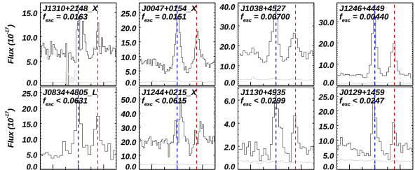
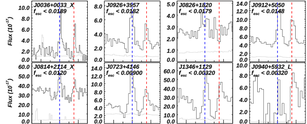
Figure 2: Same as Figure 1 but for galaxies with lower f${}_{\text{esc}}^{\text{ LyC}}$. Upper limits of f${}_{\text{esc}}^{\text{ LyC}}$ are presented for galaxies that have non-detections of LyC flux (Flury et al. 2022a). From LCEs to non-LCEs, Mg ii line profiles show a clear transition from strong emission lines to P-Cygni profiles to strong absorption lines. See more discussion in Section 3.1.

2.2 Optical Spectra for Mg ii Regions

The galaxies in the LzLCS sample already have SDSS or BOSS spectra, where the blue wavelength coverages end at 3800 Å and 3650 Å, respectively. Thus, the Mg ii features are observed by SDSS or BOSS only for galaxies with z $\gtrsim$ 0.35 or 0.30, respectively. Even for the cases with existing Mg ii spectra from SDSS/BOSS, as discussed in Xu et al. (2022), the S/N of the intrinsically weak Mg ii lines and the spectral resolution ($\sim$ 1500) are commonly too low. In this case, the measurements of Mg ii, especially $R$, have large error bars. Therefore, we have obtained higher S/N and higher spectral resolution observations for 34 galaxies from the LzLCS sample. These galaxies are observed by either the Multiple Mirror Telescope (MMT) or the Very Large Telescope (VLT), or the Hobby-Eberly Telescope (HET). In this paper, we focus on studying the Mg ii properties from this subsample of 34 galaxies. The observation details and data reductions are listed in Table 1 and discussed below.

2.2.1 MMT observations and Data Reductions

A total of 24 galaxies from the LzLCS sample have been observed by MMT. We adopt the blue channel spectrograph using a 1″ slit with the 832 lines/mm grating at the second order. This leads to a spectral resolution of $\sim$ 1 Å ($\sim$ 90 km s^-1 near the Mg ii region). The observations were conducted on 6 nights in 3 different semesters (2019A, 2020A, 2021A). The exposure time is between 30 mins to 180 mins, depending on the brightness of the target (Table 1). We stay towards lower airmass ($\lesssim$ 1.3) and, for every exposure, we reset the slit at the parallactic angle. We reduce the data following the methodology described in Henry et al. (2018) using IDL + IRAF routines. The wavelength calibration is applied from the HeArHgCd arc lamps. By matching the arc lines, we find the root-mean-square of the residuals is $<$ 0.1 Å ($\sim$ 10 km ^-1 around Mg ii spectral regions).

Given the short wavelength coverage of the blue channel spectrograph in MMT ($\sim$ 3100 – 4100 Å), the only major line covered is the Mg ii doublet. Therefore, we also adopt SDSS/BOSS spectra for measuring other optical lines (Section 2.3). For each galaxy, we calculate its u-band magnitude from the MMT spectra and scale it to the galaxy’s u-band magnitude from the SDSS photometry. This accounts for any slit losses between MMT and SDSS observations.

2.2.2 VLT observations and Data Reductions

We also include 10 LzLCS sources observed by the X-Shooter spectrograph mounted on VLT as part of the ESO program ID 106.215K.001 (PI: Schaerer). Observations were carried out between Fall 2020 and Spring 2022. We use 1.0″, 0.9″, and 0.9″ slits in the UVB, VIS and NIR arms providing resolution power of $\sim$ 5400, 8900, and 5600, respectively. This yields a spectral resolution of $\sim$ 50 km s^-1 near the Mg ii regions. Observations were performed in nodding-on-slit mode with a standard ABBA sequence and total on-source exposure times of 46 mins or 92 min, depending on the brightness of each source (Table 1). We reduce X-Shooter data following the methods in Marques-Chaves et al. (2022a) adopting the standard ESO Reflex reduction pipeline (version 2.11.5, Freudling et al. 2013).

For each galaxy, we also calculate the u-band magnitude from the VLT spectra and match it to the galaxy’s u-band magnitude from the SDSS photometry. Four of our galaxies are observed by both MMT and VLT. We have checked that the Mg ii spectral profiles from the two telescopes are similar, and the Mg ii line flux ratio (i.e., R) are consistent within errors. This is expected since galaxies in our sample are rather compact (with UV half-light-radius $\lesssim$ 0.4″) and are smaller than the slit sizes. We finally adopt these galaxies’ VLT observations in our analyses, given their higher S/N.

2.2.3 HET observations and Data Reductions

We include 4 additional galaxies from the LzLCS sample, which are observed by the Low-Resolution Spectrograph (LRS2) on the Hobby-Eberly Telescope (Ramsey et al. 1998). LRS2 is an integral field spectrograph with nearly complete spatial sampling, and a native spatial scale of 0.25″ $\times$ 0.25″ spaxels with an average of 1.25″ seeing (Chonis et al. 2016). LRS2 has a wavelength coverage from 3600 Å to 10,000 Å, and its spectral resolution around Mg ii region is 1.63 Å. To match our MMT and VLT slit sizes, we extract the Mg ii spectra in the central 1.0″ $\times$ 1.0″ aperture. We reduce the LRS2 data using the same methods in Seive et al. (2022), where we adopt the HET LRS2 pipeline, Panacea, to perform the initial reductions, including fiber extraction, wavelength, calibration, astrometry, and flux calibration. For each galaxy, we also calculate the u-band magnitude from the LRS2 spectra and match it to the galaxy’s u-band magnitude from the SDSS photometry.

2.2.4 Summary of Optical Spectra

Overall, we obtained higher-quality data for 34 out of 66 galaxies from the LzLCS sample. We show the final reduced Mg ii spectra for these galaxies in Figures 1 and 2, and have ordered them by decreasing absolute escape fraction of LyC (f${}_{\text{esc}}^{\text{ LyC}}$) measured from fitting the UV continuum (reported in Flury et al. 2022a). Based on their LyC measurements, these galaxies have f${}_{\text{esc}}^{\text{ LyC}}$ range between 0 and 30%. Of the 34 galaxies, 20 are classified as Lyman continuum emitters (LCEs, sometimes referred as LyC “leakers”), which have LyC flux detected with 97.725% confidence (Flury et al. 2022a). The other 12 galaxies are classified as non-LCEs. We show the derived f${}_{\text{esc}}^{\text{ LyC}}$ values at the top-left corners of each panel, while we present f${}_{\text{esc}}^{\text{ LyC}}$ upper limits for non-LCEs. We mark the galaxies observed by X-Shooter or LRS2 with an extra ‘X’ or ‘L’, respectively, at the end of their object names in Figures 1 and 2.

2.3 Measurements of Optical Emission Lines

For galaxies that have new optical spectra as described above, we measure several optical emission lines whenever covered, including Mg ii, [O ii], [O iii], and Balmer lines. For each galaxy, we first correct the spectra for Milky Way extinction using the Galactic Dust Reddening and Extinction Map (Schlafly & Finkbeiner 2011) at NASA/IPAC Infrared Science Archive, assuming the extinction law from Cardelli et al. (1989). The redshift of the galaxy is matched to the peak of Balmer emission lines.

We determine the continuum flux for the Mg ii spectral region by adopting a linear fit to the spectra $\sim$ $\pm$ 2000 km s^-1 around the systemic velocity. Then we split the spectra at the midpoint between the two lines, i.e., 2799.1 Å, to represent the spectral regions for 2796 and 2803, separately. For each Mg ii line, we also split it into the absorption (below the continuum) and emission (above the continuum) parts. After that, we integrate the separate spectral regions to get the flux and EW. The corresponding errors on these quantities are estimated through a Monte Carlo (MC) simulation where we perturb the spectrum 10⁴ times according to the observed 1$\sigma$ uncertainties. These values are reported in Table 2. Note that we do not correct the Mg ii line fluxes by internal dust extinction of the galaxy. This is because Mg ii photons are resonantly scattered like Ly$\alpha$ and robust correction is difficult (Henry et al. 2018; Chisholm et al. 2020; Xu et al. 2022).

For other optical lines, we measure their flux and EW similarly as Mg ii. However, unlike Mg ii, since they are not resonant lines, we also correct the spectra by the internal dust extinction for the galaxy before the measurements. The internal dust extinction ($E(B-V)_{\text{int.}}$) for each galaxy is measured from Balmer lines following the methods in Xu et al. (2022). For galaxies that only have new MMT observations, since the MMT blue channel does not cover the Balmer lines, we adopt $E(B-V)_{\text{int.}}$ derived in Flury et al. (2022a) based on their SDSS spectra. The final $E(B-V)_{\text{int.}}$ values are reported in the last column in Table 1.

In Figure 3, we compare the sub-sample adopted in this paper (red) to the rest of the galaxies in LzLCS (gray). We show two general observables that can be measured at high-redshift, including O32 = flux ratio of [O iii] $\lambda$5007/[O iii] $\lambda$3727 and stellar mass derived from spectral energy distribution (SED) fitting reported in Flury et al. (2022a). Our sub-sample of galaxies is randomly selected from the LzLCS parent sample to ensure a large dynamic range in galaxy properties.

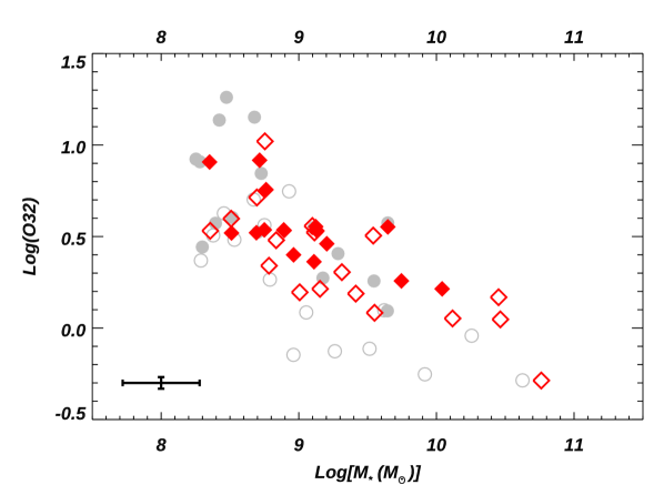
Figure 3: Comparisons of the sub-sample studied in this paper (red) to the other galaxies in the LzLCS parent sample (gray, see Section 2). Gray-filled and open symbols stand for galaxies from LzLCS, which are classified as LyC emitter and non-emitters, respectively (Flury et al. 2022a). Red-filled and open symbols represent galaxies that are Mg ii emitter and non-emitters, respectively (see definitions in Section 3.2). The mean 1$\sigma$ error bars are shown at the bottom-left of the panel.

3 Analyses

In this section, we present the methodology to derive important properties from Mg ii lines. We first discuss the significant trends in Mg ii line profiles in Section 3.1. Then we show the plausible geometry for Mg ii photon escape in Section 3.2. We present the methods to derive the Mg ii escape fractions (f${}_{\text{esc}}^{\text{ MgII}}$) from photoionization models in Section 3.3. Finally, we discuss how to predict the escape fraction of LyC (f${}_{\text{esc,pd}}^{\text{ LyC}}$) from Mg ii, metallicity, and dust attenuation in Section 3.4.

3.1 Significant Trends of Mg ii Line Profiles

In Figures 1 and 2, we show the Mg ii spectra from our galaxies in the order of decreasing f${}_{\text{esc}}^{\text{ LyC}}$ derived from HST/COS G140L spectra (Flury et al. 2022a). There exist a significant trend that galaxies detected as strong LCEs also show strong Mg ii emission lines, and non-LCEs present more absorption features in Mg ii. We apply the Kendall $\tau$ test between EW(Mg ii) and f${}_{\text{esc}}^{\text{ LyC}}$, where we have considered the upper limits following Akritas & Siebert (1996). This leads to the probability of a spurious correlation, $p$ = 0.0216, which confirms the strong trend. The former half of this trend is consistent with previous observations of strong LCEs (Izotov et al. 2022; Xu et al. 2022). Nonetheless, our sample is the first to show that this trend indeed extends to non-LCEs. This can be explained as LCEs have more optically thin clouds in/around the galaxy than non-LCEs, so both the Mg ii and LyC photons can escape with less absorption and scattering (Chisholm et al. 2022). This is also consistent with the expectations from simulations (Katz et al. 2022).

Notably, a high f${}_{\text{esc}}^{\text{ LyC}}$ (= 16.1%) was measured for galaxy J0917+3152, but its Mg ii profiles also have clear absorption features. This can be explained by the high metallicity of J0917+3152, i.e., 12+log(O/H) = 8.46, which is the highest in our sample. Thus, for this object, there exist more magnesium atoms given the same amount of hydrogen atoms. In this scenario, the clouds around J0917+3152 become optically thick to Mg ii when it is still optically thin to LyC photons. Overall, the significant trend for Mg ii profiles from LCEs to non-LCEs is valid for galaxies with lower metallicity (in our case, 12+log(O/H) $<$ 8.4). In these galaxies, the surrounding gas/clouds become optically thick to Mg ii and LyC photons at similar depths (Chisholm et al. 2020).

3.2 Possible Geometry for the Escape of Mg ii photons and Constraints on Models

The escape of Mg ii photons is first discussed in details in Chisholm et al. (2020) (hereafter, the Chisholm model, see their Section 6.4). This model assumes that Mg ii photons escape through a partial coverage geometry or sometimes referred as the picket-fence geometry (see also Gazagnes et al. 2018; Chisholm et al. 2018; Saldana-Lopez et al. 2022; Xu et al. 2022):

$$f_{\text{esc}}^{\text{Mg II}}=\frac{F_{\text{obs}}}{F_{\text{int}}}=C_{f}(\text{Mg II})e^{-\tau_{\text{thick}}}+[1-C_{f}(\text{Mg II})]e^{-\tau_{\text{thin}}}$$ (1)

where F${}_{\text{obs}}$ and F${}_{\text{int}}$ are the observed and intrinsic flux of Mg ii, respectively; C_f(Mg ii) is the covering fractions for the optically thick paths of Mg ii; and $\tau_{\text{thick}}$ and $\tau_{\text{thin}}$ are the optical depths for Mg ii at optically thick and thin paths, respectively. In the optically thick paths, it is usually assumed that $\tau_{\text{thick}}$ $\gg$ 1 such that no Mg ii photons are observed through this path. In this model, Chisholm et al. (2020) also found:

$$R=\frac{F_{\text{2796,obs}}}{F_{\text{2803,obs}}}=2e^{-\tau_{2803,thin}}$$ (2)

where $R$ is the emission line flux ratio between the Mg ii doublet. This model has proven to be successful in Chisholm et al. (2020) and Xu et al. (2022) for galaxies with strong Mg ii emissions, where Mg ii photons escape from the galaxy through mostly optically thin paths. Furthermore, Katz et al. (2022) have tested this model in their hydro-cosmological simulations for EoR galaxy analogs. They find the actual line-of-sight (LOS) f${}_{\text{esc}}^{\text{ MgII}}$ match well with the predicted ones from the Chisholm model for galaxies with low metallicity (thus less dusty) and high f${}_{\text{esc}}^{\text{ LyC}}$. These galaxies have Mg ii line profiles dominated by emission.

However, as described in Section 3.1, given the large dynamic ranges of our sample by design, our galaxies have Mg ii profiles ranging from strong emission to P-Cygni profiles and pure absorption. In the latter two cases, at least two factors complicate the applications of the Chisholm model. (1) The measurements of $R$ from the spectra are not well-defined due to the absorption in Mg ii profiles. Thus, the derived $\tau_{2803,thin}$ from $R$ has large uncertainties. (2) Mg ii doublet are resonant lines. Thus, the effect of dust for Mg ii is more substantial, which can cause strong absorption and scattering features in the spectra (e.g., J0957+2357). However, this effect cannot be described in simple terms, thus, is not included in the Chisholm model. Similarly, Katz et al. (2022) comment that the Chisholm model is likely inadequate to predict f${}_{\text{esc}}^{\text{ MgII}}$ for metal-rich (thus more dusty) galaxies in their simulations.

Currently, in this paper, to highlight the limitations of the Chisholm model, we manually split galaxies in our sample into two categories in our analyses. Galaxies with Mg ii as strong emission, minimal absorption, and symmetric line profiles are categorized as MgE (acronym for Mg ii emitter), while the others belong to non–MgE. This subjective classification is similar to what was adopted in Katz et al. (2022). The Chisholm model should apply well to the former since Mg ii photons suffer little resonant scattering effects, but not perfectly to the latter. We show the category of each galaxy in the second to last column in Table 2. We discuss further how we handle these two categories in Section 4.2.

3.3 The Method to Estimate the Escape Fraction of Mg ii

Henry et al. (2018) have first introduced that one can derive the intrinsic flux of Mg ii from a correlation between Mg ii/[O iii] and [O iii]/[O ii] (hereafter, the Henry model):

$$R_{2796} =A_{2}\times O_{32}^{2}+A_{1}\times O_{32}+A_{0}$$ (3)

$$R_{2796} =log(F_{\text{int}}(\text{Mg II }\lambda 2796)/F_{\text{int}}(\text{[O III] }\lambda 5007))$$ (4)

$$O_{32} =log(F_{\text{int}}(\text{[O III]}\ \lambda 5007)/F_{\text{int}}(\text{[O II] }\lambda 3727))$$

where the emission line fluxes are all intrinsic, i.e., before the attenuation by dust and absorption in the LOS. Hereafter, we use $F_{\text{int}}$ to denote the intrinsic flux. A₀, A₁, and A₂ are coefficients that are dependent on the gas phase metallicity of the galaxy, but little on the ionization parameters and spectral slopes (Henry et al. 2018). Combining $F_{\text{int}}$(Mg ii) with the measured $F_{\text{obs}}$(Mg ii) from the spectra, one can derive f${}_{\text{esc}}^{\text{ MgII}}$.

The photoionization models in Henry et al. (2018) considers ionization bounded (IB) geometry, where most of the cloud remains neutral and is optically thick to escaping photons. However, LCEs with strong Mg ii emission lines can be partly density bounded (DB, i.e., mostly optically thin) given their high O₃₂ values observed (e.g., Izotov et al. 2016a; b; 2018a; 2018b; 2021; Flury et al. 2022a; b; Xu et al. 2022). Thus, Xu et al. (2022) update the correlation coefficients in the Henry model to take into account the DB scenario. At a fixed metallicity, they also find the different models from DB and IB only move the correlation along the line defined in Equation (3). This should explain why Katz et al. (2022) find the Henry model is a relatively good match to galaxies in their simulations, but with moderate scatter given the different metallicities of their simulated galaxies.

Given the derived f${}_{\text{esc}}^{\text{ MgII}}$, one can solve C_f(Mg ii) and $\tau_{\text{thin}}$ from Equations (1) and (2). Note this requires robust measurements of Mg ii doublet flux ratio, i.e., $R$ in Equation (2). As discussed in Section 3.2, this can be achieved in MgE, but hardly in non–MgE due to the absorption features in Mg ii. Since C_f(Mg ii) and $\tau_{\text{thin}}$ are then adopted to predict f${}_{\text{esc}}^{\text{ LyC}}$, accurately predictions are more difficult for non–MgE (see detailed discussion in Sections 3.4 and 4.2).

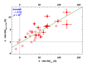
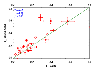
Figure 4: Correlations between Mg ii and Ly$\alpha$ properties. Galaxies that are labelled as MgE and non-MgE from our sample are shown in filled and open symbols, respectively (Section 3.2). Left: The net EW from Mg ii $\lambda$2796 and Ly$\alpha$ are positively correlated. Each galaxy is shown as a dot with the cross representing its error bars. Galaxies with strong Mg ii emission lines are at the top-right of the figure. The green dashed line represents the best linear fit. Right: The escape fraction of Mg ii $\lambda$2796 and Ly$\alpha$ are tightly correlated. The correlation coefficients from Kendall $\tau$ test are shown at the top-left corner in each panel. The green solid line represents the 1:1 correlation. See discussion in Section 4.1.

3.4 The Method to Predict the Escape Fraction of LyC

As discussed in numerous previous publications (e.g., Zackrisson et al. 2013; Reddy et al. 2016; Chisholm et al. 2020; Kakiichi & Gronke 2021; Saldana-Lopez et al. 2022), the escape of LyC photons can be described as a partial-covering geometry:

$$f_{\text{esc}}(\text{LyC}) =C_{f}(\text{H I})e^{-\tau_{\text{thick}}}\times 10^{-0.4A_{\text{thick}}}$$ (5)

$$+[1-C_{f}(\text{H I})]e^{-\tau_{\text{thin}}}\times 10^{-0.4A_{\text{thin}}}$$

where C_f(H i) is the covering fractions for optically thick paths of H i which is dominated by neutral gas, and $A_{\text{thick}}$ and $A_{\text{thin}}$ are the attenuation parameters for LyC photons at optically thick and optically thin paths, respectively.

For galaxies in our LzLCS sample, Saldana-Lopez et al. (2022) have found that the covering fraction of lower ionization lines (LIS, including O i, C ii, Si ii) trace that of H i. Given similar ionization potentials of Mg ii to these lines, we adopt their best-fit linear correlation to estimate C_f(H i) as:

$$C_{f}(\text{H I})=(0.63\pm 0.19)C_{f}(\text{Mg II})+(0.54\pm 0.09)$$ (6)

For optically thick paths, we assume no LyC photons can escape (i.e., $\tau_{\text{thick}}$ and/or $A_{\text{thick}}$ $\gg$ 1). Therefore, the first term in Equation (5) is negligible. $A_{\text{thin}}$ is related to the dust extinction at the LyC, for which we adopt the stellar extinction derived from SED fittings in Saldana-Lopez et al. (2022). They used Starburst99 template (Leitherer et al. 1999) and have assumed the extinction law from Reddy et al. (2015; 2016). Therefore, we can rewrite Equation (5) as:

$$f^{\text{LyC}}_{\text{esc,pd}}=[1-C_{f}(\text{H I})]e^{-N(\text{H I})\sigma_{ph}}\times 10^{-0.4E(B-V)k(912)}$$ (7)

where $f^{\text{LyC}}_{\text{esc,pd}}$ is the predicted absolute escape fraction of LyC, N(H i) is the column density of neutral hydrogen, $\sigma_{ph}$ is the photoionization cross section of H i at 912 Å, $E(B-V)$ is the stellar dust extinction from Saldana-Lopez et al. (2022), and k(912) is the total attenuation curve at the Lyman limit. Given the Reddy extinction law adopted in Saldana-Lopez et al. (2022), we have k(912) = 12.87. For other extinction laws, e.g., Cardelli et al. (1989) and Calzetti et al. (2000), k(912) = 21.32 and 16.62, respectively.

As shown in Chisholm et al. (2020) and Xu et al. (2022), by assuming that Mg ii and LyC photons escape from similar optically thin paths, the column density of Mg ii [i.e., N(Mg ii)] can be used to trace N(H i) in a large range from DB to nearly IB regions:

$$N(\text{H I}) =\alpha\times N(\text{Mg II})$$ (8)

where N(Mg II) can be calculated from the optical depth of Mg ii as inferred from $R$ in Section 3.2, and $\alpha$ = N(Mg ii)/N(H i) is the column density ratios predicted from CLOUDY models (Xu et al. 2022). $\alpha$ is dependent on the abundance ratio of [Mg/H] and the ionization, and has typical values $\sim$ 10⁴ – 10⁵ for galaxies in our sample. Combining Equations (5) to (8), we can calculate f${}_{\text{esc,pd}}^{\text{ LyC}}$ given the information of Mg ii, metallicity, and dust.

In $\sim$ 20 galaxies with strong Mg ii emission lines, this model predicted f${}_{\text{esc,pd}}^{\text{ LyC}}$ has been found to correlate well with the actual f${}_{\text{esc}}^{\text{ LyC}}$ measured from the spectra (Chisholm et al. 2020; Xu et al. 2022). Likewise, Katz et al. (2022) also found that f${}_{\text{esc,pd}}^{\text{ LyC}}$ correlates with the actual f${}_{\text{esc}}^{\text{ LyC}}$ for simulated high-redshift galaxies at different LOS (top-middle panel of their Figure 17). But their correlation contains a large scatter. We note that they adopt $\alpha$ as the abundance ratio of hydrogen to oxygen, i.e., $\alpha$ = 46$\frac{H}{O}$ (Chisholm et al. 2020). This assumes the Mg ii emission is found in neutral gas. This is not accurate since known LCEs commonly have high O₃₂ values and, thus, at least a fraction of the ISM (i.e., 1 - C_f(H i)) is density bounded. Therefore, Mg ii in these galaxies should originate in regions where N(H ii) is non-negligible. Our adopted $\alpha$ from CLOUDY models in Equation 8 overcomes this problem (Xu et al. 2022). In Section 4.2, we compare f${}_{\text{esc,pd}}^{\text{ LyC}}$ with the measured f${}_{\text{esc}}^{\text{ LyC}}$ from Flury et al. (2022a) based on the HST COS/G140L spectra and SED fittings.

4 Results

4.1 Estimates of the Escape Fraction of Mg ii

From Sections 3.2 to 3.3, we show how to derive f${}_{\text{esc}}^{\text{ MgII}}$. The resulting values are listed in the last column of Table 2. Furthermore, in Figure 4, we present the correlations between Mg ii and Ly$\alpha$. In the left panel, we compare the net EW (i.e., the summed EW from both emission and absorption features) between Mg ii and Ly$\alpha$. To be consistent with the literature, we have multiplied the net EW by -1 to allow galaxies with strong emission lines to be at the top-right corner, while galaxies with strong absorption lines to be at the bottom-left corner. We find a strong positive correlation between the net EW of Mg ii and Ly$\alpha$. This is as expected since both are resonant lines and should follow similar radiative transfer processes when travelling out of the galaxies. The best fit linear correlation is (show as the green dashed line):

net EW(Mg II) $$=a+b\times\text{net EW}(\text{Ly}\alpha)$$ (9)

$$a =-0.468_{-0.157}^{+0.157}$$

$$b =0.091_{-0.003}^{+0.003}$$

Similar but less significant trends between EW(Mg ii) and EW(Ly$\alpha$) have also been published in Henry et al. (2018) and Xu et al. (2022), where they only focused on strong Mg ii emitters.

In the right panel of Figure 4, we compare the derived f${}_{\text{esc}}^{\text{ MgII}}$ with the escape fraction of Ly$\alpha$ (f${}_{\text{esc}}^{\text{ Ly}\alpha}$). The latter is derived from each galaxy’s HST/COS spectra in Flury et al. (2022a). The correlation is significant ($p$ $<$ 10^-6) with scatter. We find most of the galaxies follow the 1:1 correlation shown as the solid green line, which suggests f${}_{\text{esc}}^{\text{ Ly}\alpha}$ $\simeq$ f${}_{\text{esc}}^{\text{ MgII}}$. This is consistent with the results in Henry et al. (2018) and Xu et al. (2022), which also found that f${}_{\text{esc}}^{\text{ MgII}}$ and f${}_{\text{esc}}^{\text{ Ly}\alpha}$ values are of the same order. This supports the scenario where Mg ii and Ly$\alpha$  mainly escape from optically thin (or DB) holes in ISM likely in a single flight (e.g., Gazagnes et al. 2018; Chisholm et al. 2020; Saldana-Lopez et al. 2022). Thus, the path lengths of Mg ii and Ly$\alpha$ photons travelling out of the galaxy are similar, and the resulting escape fractions are close for both lines. One possible scenario is that there is zero dust in the optically thin paths. Future spatially resolved observations can solve this puzzle. This includes our Lyman-alpha and Continuum Origins Survey (LaCOS, HST-GO 17069, PI: Hayes), which aims to spatially resolve the Ly$\alpha$ emission, dust, and stellar population for 41 out of 66 LzLCS galaxies by HST imaging.

For all figures in this section, we show Kendall $\tau$ coefficients and the probability of a spurious correlation (p values) at the top-left corner. In the Kendall test, we have accounted for the upper limits (if any) following Akritas & Siebert (1996). We have also tested the correlations between the scatters in each figure with other galaxy properties, including metallicity, internal dust extinction, SFR surface density, and stellar mass. However, we do not find significant correlations.

4.2 Estimates of the Escape Fraction of LyC from Mg ii

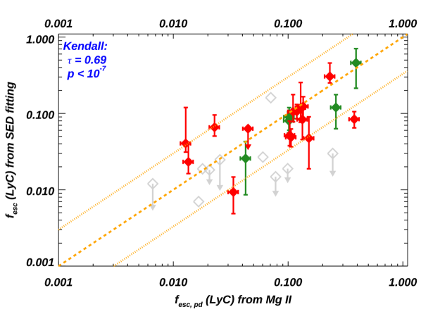
Figure 5: Comparisons of measured f${}_{\text{esc}}^{\text{ LyC}}$ with the predicted one from Mg ii $\lambda$2796 emission lines. Galaxies that are labelled as MgE and non-MgE from our sample are shown in filled-red and open-gray symbols, respectively (Section 3.2). Galaxies that are determined to be non-Lyman-continuum-emitter (Flury et al. 2022a) are shown as upper limits. The orange dotted lines are to show the factor of 3 scatter around the 1:1 relationship (orange dashed line). We also show 5 galaxies from Guseva et al. (2020) as green colors. See discussion in Section 4.2.

In Figure 5, we compare f${}_{\text{esc,pd}}^{\text{ LyC}}$ derived in Section 3.4 with the f${}_{\text{esc}}^{\text{ LyC}}$ values derived from the HST/COS spectra (based on UV continuum fittings, Flury et al. 2022a). We draw galaxies classified as MgE and non–MgE as filled and open symbols, respectively. We also include 5 galaxies from Guseva et al. (2020), which have high-quality VLT/X-Shooter observations as well as direct LyC measurements. We derive f${}_{\text{esc,pd}}^{\text{ LyC}}$ in the same way as in Section 3.4, and remeasure their f${}_{\text{esc}}^{\text{ LyC}}$ from HST/COS spectra using the same methodology in Flury et al. (2022a).

First of all, there is a strong correlation between the predicted f${}_{\text{esc}}^{\text{ LyC}}$ from Mg ii and measured ones, given the probability of a spurious correlation $p<10^{-7}$. This highlights the power of using Mg ii to trace LyC. Given the scatter around the 1:1 relationships line (orange dashed line), our predicted f${}_{\text{esc}}^{\text{ LyC}}$ values are accurate within a factor of 3. Considering only the non-MgEs (gray-open symbols), the correlation is less significant. This can be because their Mg ii emission lines are affected by absorption features, and the derived $\tau_{2803,thin}$ and C_f(Mg ii) from Equation (2) is more uncertain.

For some of the non–MgE, their Mg ii spectra show significant resonant scattering or absorption signatures. These include galaxies showing double peaks in each Mg ii emission lines (J1310+2148, J1244+0215, J0826+1820, and maybe in J1235+0635), and galaxies showing strong absorption in Mg ii (J0723+4146, J0940+5932, J1346+1129, J1314+1048, J0957+2357). These galaxies should have optically thicker clouds in/around the galaxy, and our measurements of emission line flux of Mg ii are also uncertain. Thus, no meaningful predictions through Mg ii emission lines can be made, and we have excluded these galaxies from Figure 5. We note that, among these galaxies, only one (J1310+2148, f${}_{\text{esc}}^{\text{ LyC}}$ $\sim$ 1.6%) has small amount of LyC detected from HST/COS spectra, and others show non-detections of LyC (see Figures 1 and 2). Thus, these non-MgEs are more similar to galaxies that are cosmologically irrelevant to EoR (f${}_{\text{esc}}^{\text{ LyC}}$ $\ll$ 1%). Therefore, precise estimates of their f${}_{\text{esc}}^{\text{ LyC}}$ are less important for our understanding of SF galaxies contributing to the reionization. Furthermore, when selecting new LyC emitters for future observations, one can also exclude similar non-MgEs based on the absorption and/or scattering features in Mg ii line profiles.

In the future, we plan to perform detailed radiative transfer models to account for the escape of Mg ii out of the galaxy and link it to the escape of Ly$\alpha$ and LyC (Carr et al. in preparation). We can then model and separate the emission and absorption features from the observed Mg ii spectra. This will be particularly helpful to make more realistic predictions of f${}_{\text{esc,pd}}^{\text{ LyC}}$ for these galaxies labelled as non–MgE.

Overall, our derived f${}_{\text{esc,pd}}^{\text{ LyC}}$ from Mg ii, metallicity, and dust can correctly trace the measured f${}_{\text{esc}}^{\text{ LyC}}$ within a factor of $\sim$ 3 for MgE. This is consistent with previous studies in Chisholm et al. (2020); Xu et al. (2022). We conclude that Mg ii emission lines along with dust can be used to predict the escape of LyC photons in MgEs, but we need additional information to do so in non-MgEs (e.g., detailed radiative transfer models).

Table 2: Measurements from Optical Spectra for the Comparison Sample

Object	O32	O/H	F${}_{2796}^{Emi}$	F${}_{2803}^{Emi}$	—EW${}_{2796}^{Emi}$—	—EW${}_{2803}^{Emi}$—	—EW${}_{2796}^{Abs}$—	—EW${}_{2803}^{Abs}$—	Label	f${}_{\text{esc}}^{\text{ MgII}}$
(a)	(b)	(c)	(d)	(e)	(f)	(g)	(h)	(i)	(j)	(k)
J1033+6353	3.4	8.2	50.2$\pm{7.0}$	34.9$\pm{7.0}$	4.7$\pm{0.8}$	3.6$\pm{0.8}$	0.9$\pm{0.3}$	0.0$\pm{0.0}$	MgE	0.29$\pm{0.04}$
J0917+3152	2.0	8.5	16.2$\pm{7.4}$	13.5$\pm{6.8}$	1.1$\pm{0.4}$	0.9$\pm{0.6}$	1.2$\pm{0.4}$	0.9$\pm{0.3}$	non-MgE	0.06$\pm{0.03}$
J1327+4218	3.3	8.2	38.2$\pm{4.4}$	22.7$\pm{4.8}$	6.0$\pm{0.6}$	4.1$\pm{1.2}$	0.3$\pm{0.08}$	0.5$\pm{0.1}$	MgE	0.18$\pm{0.02}$
J1410+4345	8.3	8.0	10.8$\pm{2.4}$	7.8$\pm{2.6}$	7.3$\pm{1.6}$	5.6$\pm{2.0}$	0.3$\pm{0.09}$	0.0$\pm{0.0}$	MgE	0.13$\pm{0.03}$
J1158+3125	1.8	8.4	75.5$\pm{5.2}$	38.6$\pm{4.8}$	3.2$\pm{0.2}$	1.7$\pm{0.2}$	0.6$\pm{0.2}$	0.3$\pm{0.09}$	MgE	0.18$\pm{0.01}$
J1235+0635	3.4	8.4	16.1$\pm{1.6}$	10.6$\pm{1.4}$	2.3$\pm{0.2}$	1.5$\pm{0.2}$	0.5$\pm{0.1}$	0.0$\pm{0.0}$	MgE	0.16$\pm{0.02}$
J1248+1234	3.4	8.2	116.3$\pm{5.0}$	62.3$\pm{4.6}$	9.6$\pm{0.6}$	5.0$\pm{0.4}$	1.3$\pm{0.4}$	0.5$\pm{0.1}$	MgE	0.44$\pm{0.02}$
J1517+3705	2.5	8.3	41.8$\pm{1.2}$	26.7$\pm{1.4}$	7.4$\pm{0.4}$	4.2$\pm{0.2}$	1.2$\pm{0.2}$	0.7$\pm{0.2}$	MgE	0.12$\pm{0.003}$
J0122+0520	5.7	7.8	27.7$\pm{2.6}$	17.5$\pm{2.4}$	6.4$\pm{1.0}$	4.8$\pm{1.2}$	0.1$\pm{0.03}$	0.3$\pm{0.09}$	MgE	0.59$\pm{0.06}$
J1301+5104	3.3	8.3	31.4$\pm{5.6}$	16.4$\pm{5.0}$	5.0$\pm{0.8}$	3.1$\pm{1.0}$	0.7$\pm{0.2}$	0.3$\pm{0.09}$	non-MgE	0.18$\pm{0.03}$
J1648+4957	3.3	8.2	35.4$\pm{0.4}$	23.9$\pm{0.4}$	21.3$\pm{0.2}$	16.1$\pm{0.2}$	3.5$\pm{0.2}$	0.0$\pm{0.0}$	MgE	0.49$\pm{0.006}$
J0911+1831	1.6	8.1	50.4$\pm{7.4}$	34.4$\pm{8.2}$	2.9$\pm{0.4}$	2.0$\pm{0.4}$	1.0$\pm{0.3}$	0.5$\pm{0.2}$	MgE	0.12$\pm{0.02}$
J0113+0002	2.3	8.3	42.9$\pm{3.0}$	23.1$\pm{2.6}$	5.0$\pm{0.6}$	2.9$\pm{0.4}$	1.1$\pm{0.3}$	0.5$\pm{0.1}$	MgE	0.59$\pm{0.04}$
J1133+4514	3.6	8.0	83.9$\pm{6.4}$	43.1$\pm{6.6}$	7.3$\pm{0.6}$	3.8$\pm{0.6}$	0.1$\pm{0.04}$	0.0$\pm{0.0}$	MgE	0.65$\pm{0.05}$
J0811+4141	8.1	7.9	45.7$\pm{4.2}$	28.0$\pm{4.0}$	12.9$\pm{1.2}$	7.4$\pm{1.0}$	1.0$\pm{0.3}$	0.0$\pm{0.0}$	MgE	1.00$\pm{0.23}$
J0958+2025	5.2	7.8	21.2$\pm{5.0}$	8.4$\pm{4.2}$	8.2$\pm{2.6}$	4.4$\pm{2.8}$	2.2$\pm{0.7}$	0.5$\pm{0.1}$	non-MgE	0.11$\pm{0.03}$
J1310+2148	1.6	8.4	18.7$\pm{2.0}$	12.4$\pm{1.6}$	2.1$\pm{0.4}$	1.4$\pm{0.2}$	1.6$\pm{0.5}$	0.3$\pm{0.09}$	non-MgE	0.06$\pm{0.007}$
J0047+0154	2.9	8.0	41.8$\pm{2.8}$	31.0$\pm{3.0}$	4.0$\pm{0.2}$	3.1$\pm{0.2}$	1.3$\pm{0.2}$	0.8$\pm{0.2}$	MgE	0.23$\pm{0.02}$
J1038+4527	1.5	8.4	59.9$\pm{8.4}$	35.4$\pm{9.0}$	2.8$\pm{0.4}$	1.7$\pm{0.4}$	0.8$\pm{0.2}$	0.6$\pm{0.2}$	non-MgE	0.14$\pm{0.02}$
J1246+4449	3.4	8.0	72.4$\pm{4.2}$	41.4$\pm{4.0}$	10.8$\pm{0.6}$	6.2$\pm{0.6}$	0.5$\pm{0.2}$	0.1$\pm{0.04}$	MgE	0.29$\pm{0.02}$
J0834+4805	3.6	8.2	55.6$\pm{1.4}$	44.7$\pm{1.4}$	7.4$\pm{0.4}$	6.1$\pm{0.2}$	1.0$\pm{0.2}$	0.0$\pm{0.0}$	MgE	0.09$\pm{0.002}$
J1244+0215	3.6	8.2	64.3$\pm{7.6}$	40.4$\pm{7.4}$	2.8$\pm{0.6}$	1.8$\pm{0.6}$	0.7$\pm{0.2}$	0.5$\pm{0.2}$	non-MgE	0.08$\pm{0.009}$
J1130+4935	3.4	8.3	15.2$\pm{2.0}$	7.4$\pm{1.8}$	6.3$\pm{0.8}$	3.1$\pm{0.8}$	1.5$\pm{0.4}$	0.9$\pm{0.3}$	non-MgE	0.38$\pm{0.05}$
J0129+1459	1.6	8.4	33.7$\pm{7.6}$	15.8$\pm{8.2}$	3.3$\pm{0.8}$	1.7$\pm{1.2}$	1.8$\pm{0.5}$	1.2$\pm{0.4}$	non-MgE	0.17$\pm{0.04}$
J0036+0033	10.5	7.8	14.4$\pm{2.2}$	7.5$\pm{2.8}$	7.7$\pm{1.8}$	5.3$\pm{2.4}$	1.3$\pm{0.4}$	1.0$\pm{0.3}$	non-MgE	0.20$\pm{0.03}$
J0926+3957	2.2	8.2	12.3$\pm{2.2}$	6.1$\pm{1.8}$	4.1$\pm{0.8}$	1.8$\pm{0.6}$	0.8$\pm{0.3}$	1.0$\pm{0.3}$	non-MgE	0.17$\pm{0.03}$
J0826+1820	4.0	8.3	7.5$\pm{2.6}$	3.4$\pm{2.2}$	2.8$\pm{1.0}$	1.8$\pm{1.4}$	0.4$\pm{0.1}$	1.2$\pm{0.4}$	non-MgE	0.12$\pm{0.04}$
J0912+5050	3.0	8.2	25.3$\pm{3.2}$	19.6$\pm{3.6}$	4.4$\pm{0.6}$	3.5$\pm{0.6}$	0.4$\pm{0.1}$	0.1$\pm{0.04}$	non-MgE	0.21$\pm{0.03}$
J0814+2114	1.2	8.1	39.4$\pm{9.2}$	28.7$\pm{10.0}$	1.4$\pm{0.4}$	0.9$\pm{0.4}$	0.7$\pm{0.2}$	0.3$\pm{0.08}$	non-MgE	0.06$\pm{0.01}$
J0723+4146	3.2	8.2	27.6$\pm{6.4}$	16.9$\pm{6.6}$	4.9$\pm{1.2}$	3.6$\pm{1.6}$	1.6$\pm{0.5}$	0.9$\pm{0.3}$	non-MgE	0.33$\pm{0.08}$
J0940+5932	1.5	8.4	…	…	…	…	5.9$\pm{0.2}$	4.2$\pm{0.4}$	non-MgE	…
J1346+1129	1.1	8.3	72.1$\pm{11.0}$	68.7$\pm{12.8}$	2.3$\pm{0.4}$	2.2$\pm{0.6}$	2.6$\pm{0.4}$	2.3$\pm{0.4}$	non-MgE	0.11$\pm{0.02}$
J1314+1048	1.1	8.3	25.0$\pm{5.6}$	27.4$\pm{8.0}$	1.4$\pm{0.2}$	1.5$\pm{0.6}$	3.0$\pm{0.4}$	2.2$\pm{0.4}$	non-MgE	0.05$\pm{0.01}$
J0957+2357	0.5	8.4	…	…	…	…	2.9$\pm{0.4}$	2.6$\pm{0.4}$	non-MgE	…
Note. –Measurements from the optical spectra for galaxies in our sample. Galaxies are ordered by decreasing f${}_{\text{esc}}^{\text{ LyC}}$ derived in Flury et al. (2022a) (the same order as Figures 1 and 2). The columns are: (b) Flux ratio between [O iii] $\lambda$5007 and [O ii] $\lambda$3727; (c) Gas phase metallicity in the form of 12+log(O/H); (d) and (e) Measured emission line flux of Mg ii $\lambda$$\lambda$2796, 2803 lines in units of 10-17 ergs s-1 cm-2, respectively; (f) and (g): Measured rest-frame EW in units of Å for the emission part from the Mg ii doublet (see Section 2.3); (h) and (i) Measured rest-frame EW in units of Å for the absorption part from the Mg ii doublet; (j) Labels based on the Mg ii line profiles, i.e., MgE = Mg ii emitter, non-MgE = Mg ii non-emitter (see Section 3.2); and (k): the derived escape fraction for Mg ii $\lambda$2796 (see Section 3.3).

5 Conclusion and Future Work

We present the analyses of Mg ii spectra for 34 galaxies chosen from the LzLCS sample. These galaxies have published HST/COS data for their LyC and Ly$\alpha$ spectral regions, and we have obtained higher S/N and resolution spectra (than SDSS) for their Mg ii regions.

While previous studies of Mg ii in Lyman Continuum Emitter (LCE) candidates have only focused on Mg ii emitters (MgE), galaxies in our sample have Mg ii profiles ranging from strong emission to P-Cygni profiles, then to pure absorption. We find there is a significant trend ($p$ = 0.0216) that galaxies detected as strong LCEs show larger EW(Mg ii) in emission lines, while non-LCEs present larger EW(Mg ii) in absorption.

We discuss the picket-fence geometry for the escape of Mg ii photons from galaxies. While this geometry has been found to apply well to galaxies categorized as MgE, it has limitations in the case of non-MgE. We then discuss how to use the CLOUDY photoionization models to help derive the escape fraction of Mg ii (f${}_{\text{esc}}^{\text{ MgII}}$) from the optical spectra. For all galaxies in our sample, we find f${}_{\text{esc}}^{\text{ MgII}}$ correlates with the escape fraction of Ly$\alpha$. We also show that the net equivalent width of Mg ii and Ly$\alpha$ are tightly correlated for both MgEs and non-MgEs.

We also discuss the methods to predict the escape fraction of LyC (f${}_{\text{esc,pd}}^{\text{ LyC}}$) from the measurements of Mg ii, metallicity, and dust. We show that the predicted f${}_{\text{esc,pd}}^{\text{ LyC}}$ correlates well with the actual f${}_{\text{esc}}^{\text{ LyC}}$ derived from the HST/COS spectra within a factor of $\sim$ 3. For non-MgEs, the correlation is less significant. This is because the absorption features in Mg ii spectra for non-MgE complicate our measurements of Mg ii emission lines. Additional information, e.g., from radiative transfer models, may help solve this problem.

In the future, one can apply the Mg ii correlations to various different studies, including: 1). We will perform detailed radiative transfer models to account for the escape of Mg ii from the galaxy (Carr et al. in preparation). This will be especially helpful for the cases of non-MgE, where the clouds in/around the galaxy are not optically thin to Mg ii. 2) For high-z galaxies, one can adopt the observed Mg ii features to estimate the intrinsic amount of Ly$\alpha$, which can be severely attenuated by the neutral IGM (e.g., Mason et al. 2018). Thus, with the aid of Mg ii, one can get more accurate estimates of the IGM neutral fractions from Ly$\alpha$. 3). One can conduct similar analyses of Mg ii in higher-redshift LCE candidates, whose Mg ii emission lines are shifted into the observable bands of the James Webb Space Telescope (JWST). The Ly$\alpha$–Mg ii correlations can be adopted to select Ly$\alpha$ emitters that have detectable Mg ii spectra, and the Mg ii–LyC correlation can be used to predict f${}_{\text{esc}}^{\text{ LyC}}$ in the case when LyC cannot be directly detected.

References

- Akritas & Siebert (1996) Akritas, M. G., & Siebert, J. 1996, MNRAS, 278, 919, doi: 10.1093/mnras/278.4.919
- Becker et al. (2021) Becker, G. D., D’Aloisio, A., Christenson, H. M., et al. 2021, MNRAS, 508, 1853, doi: 10.1093/mnras/stab2696
- Begley et al. (2022) Begley, R., Cullen, F., McLure, R. J., et al. 2022, MNRAS, 513, 3510, doi: 10.1093/mnras/stac1067
- Bergvall et al. (2006) Bergvall, N., Zackrisson, E., Andersson, B. G., et al. 2006, A&A, 448, 513, doi: 10.1051/0004-6361:20053788
- Bian et al. (2017) Bian, F., Fan, X., McGreer, I., Cai, Z., & Jiang, L. 2017, ApJ, 837, L12, doi: 10.3847/2041-8213/aa5ff7
- Borthakur et al. (2014) Borthakur, S., Heckman, T. M., Leitherer, C., & Overzier, R. A. 2014, Science, 346, 216, doi: 10.1126/science.1254214
- Bosman et al. (2022) Bosman, S. E. I., Davies, F. B., Becker, G. D., et al. 2022, MNRAS, 514, 55, doi: 10.1093/mnras/stac1046
- Boyett et al. (2022) Boyett, K., Mascia, S., Pentericci, L., et al. 2022, arXiv e-prints, arXiv:2207.13459. https://arxiv.org/abs/2207.13459
- Calzetti et al. (2000) Calzetti, D., Armus, L., Bohlin, R. C., et al. 2000, ApJ, 533, 682, doi: 10.1086/308692
- Cardelli et al. (1989) Cardelli, J. A., Clayton, G. C., & Mathis, J. S. 1989, ApJ, 345, 245, doi: 10.1086/167900
- Chisholm et al. (2020) Chisholm, J., Prochaska, J. X., Schaerer, D., Gazagnes, S., & Henry, A. 2020, MNRAS, 498, 2554, doi: 10.1093/mnras/staa2470
- Chisholm et al. (2018) Chisholm, J., Tremonti, C., & Leitherer, C. 2018, MNRAS, 481, 1690, doi: 10.1093/mnras/sty2380
- Chisholm et al. (2022) Chisholm, J., Saldana-Lopez, A., Flury, S., et al. 2022, MNRAS, 517, 5104, doi: 10.1093/mnras/stac2874
- Chonis et al. (2016) Chonis, T. S., Hill, G. J., Lee, H., et al. 2016, in Society of Photo-Optical Instrumentation Engineers (SPIE) Conference Series, Vol. 9908, Ground-based and Airborne Instrumentation for Astronomy VI, ed. C. J. Evans, L. Simard, & H. Takami, 99084C, doi: 10.1117/12.2232209
- de Barros et al. (2016) de Barros, S., Vanzella, E., Amor ́in, R., et al. 2016, A&A, 585, A51, doi: 10.1051/0004-6361/201527046
- Dijkstra et al. (2016) Dijkstra, M., Gronke, M., & Venkatesan, A. 2016, ApJ, 828, 71, doi: 10.3847/0004-637X/828/2/71
- Erb et al. (2012) Erb, D. K., Quider, A. M., Henry, A. L., & Martin, C. L. 2012, ApJ, 759, 26, doi: 10.1088/0004-637X/759/1/26
- Ferland et al. (2017) Ferland, G. J., Chatzikos, M., Guzmán, F., et al. 2017, Rev. Mexicana Astron. Astrofis., 53, 385. https://arxiv.org/abs/1705.10877
- Finley et al. (2017) Finley, H., Bouché, N., Contini, T., et al. 2017, A&A, 605, A118, doi: 10.1051/0004-6361/201730428
- Fletcher et al. (2019) Fletcher, T. J., Tang, M., Robertson, B. E., et al. 2019, ApJ, 878, 87, doi: 10.3847/1538-4357/ab2045
- Flury et al. (2022a) Flury, S. R., Jaskot, A. E., Ferguson, H. C., et al. 2022a, ApJS, 260, 1, doi: 10.3847/1538-4365/ac5331
- Flury et al. (2022b) —. 2022b, ApJ, 930, 126, doi: 10.3847/1538-4357/ac61e4
- Freudling et al. (2013) Freudling, W., Romaniello, M., Bramich, D. M., et al. 2013, A&A, 559, A96, doi: 10.1051/0004-6361/201322494
- Gazagnes et al. (2020) Gazagnes, S., Chisholm, J., Schaerer, D., Verhamme, A., & Izotov, Y. 2020, A&A, 639, A85, doi: 10.1051/0004-6361/202038096
- Gazagnes et al. (2018) Gazagnes, S., Chisholm, J., Schaerer, D., et al. 2018, A&A, 616, A29, doi: 10.1051/0004-6361/201832759
- Gronke et al. (2021) Gronke, M., Ocvirk, P., Mason, C., et al. 2021, MNRAS, 508, 3697, doi: 10.1093/mnras/stab2762
- Guseva et al. (2020) Guseva, N. G., Izotov, Y. I., Schaerer, D., et al. 2020, MNRAS, 497, 4293, doi: 10.1093/mnras/staa2197
- Hayes et al. (2021) Hayes, M. J., Runnholm, A., Gronke, M., & Scarlata, C. 2021, ApJ, 908, 36, doi: 10.3847/1538-4357/abd246
- Heckman et al. (2001) Heckman, T. M., Sembach, K. R., Meurer, G. R., et al. 2001, ApJ, 558, 56, doi: 10.1086/322475
- Henry et al. (2018) Henry, A., Berg, D. A., Scarlata, C., Verhamme, A., & Erb, D. 2018, ApJ, 855, 96, doi: 10.3847/1538-4357/aab099
- Henry et al. (2015) Henry, A., Scarlata, C., Martin, C. L., & Erb, D. 2015, ApJ, 809, 19, doi: 10.1088/0004-637X/809/1/19
- Inoue et al. (2014) Inoue, A. K., Shimizu, I., Iwata, I., & Tanaka, M. 2014, MNRAS, 442, 1805, doi: 10.1093/mnras/stu936
- Izotov et al. (2022) Izotov, Y. I., Chisholm, J., Worseck, G., et al. 2022, MNRAS, 515, 2864, doi: 10.1093/mnras/stac1899
- Izotov et al. (2016a) Izotov, Y. I., Orlitová, I., Schaerer, D., et al. 2016a, Nature, 529, 178, doi: 10.1038/nature16456
- Izotov et al. (2016b) Izotov, Y. I., Schaerer, D., Thuan, T. X., et al. 2016b, MNRAS, 461, 3683, doi: 10.1093/mnras/stw1205
- Izotov et al. (2018a) Izotov, Y. I., Schaerer, D., Worseck, G., et al. 2018a, MNRAS, 474, 4514, doi: 10.1093/mnras/stx3115
- Izotov et al. (2021) Izotov, Y. I., Worseck, G., Schaerer, D., et al. 2021, MNRAS, 503, 1734, doi: 10.1093/mnras/stab612
- Izotov et al. (2018b) —. 2018b, MNRAS, 478, 4851, doi: 10.1093/mnras/sty1378
- Jaskot et al. (2019) Jaskot, A. E., Dowd, T., Oey, M. S., Scarlata, C., & McKinney, J. 2019, ApJ, 885, 96, doi: 10.3847/1538-4357/ab3d3b
- Ji et al. (2020) Ji, Z., Giavalisco, M., Vanzella, E., et al. 2020, ApJ, 888, 109, doi: 10.3847/1538-4357/ab5fdc
- Kakiichi & Gronke (2021) Kakiichi, K., & Gronke, M. 2021, ApJ, 908, 30, doi: 10.3847/1538-4357/abc2d9
- Katz et al. (2022) Katz, H., Garel, T., Rosdahl, J., et al. 2022, MNRAS, doi: 10.1093/mnras/stac1437
- Le Reste et al. (2022) Le Reste, A., Hayes, M., Cannon, J. M., et al. 2022, ApJ, 934, 69, doi: 10.3847/1538-4357/ac77ed
- Leitet et al. (2013) Leitet, E., Bergvall, N., Hayes, M., Linné, S., & Zackrisson, E. 2013, A&A, 553, A106, doi: 10.1051/0004-6361/201118370
- Leitherer et al. (2016) Leitherer, C., Hernandez, S., Lee, J. C., & Oey, M. S. 2016, ApJ, 823, 64, doi: 10.3847/0004-637X/823/1/64
- Leitherer et al. (1999) Leitherer, C., Schaerer, D., Goldader, J. D., et al. 1999, ApJS, 123, 3, doi: 10.1086/313233
- Marchi et al. (2017) Marchi, F., Pentericci, L., Guaita, L., et al. 2017, A&A, 601, A73, doi: 10.1051/0004-6361/201630054
- Marchi et al. (2018) —. 2018, A&A, 614, A11, doi: 10.1051/0004-6361/201732133
- Marques-Chaves et al. (2022a) Marques-Chaves, R., Schaerer, D., Amor ́in, R. O., et al. 2022a, arXiv e-prints, arXiv:2205.05567. https://arxiv.org/abs/2205.05567
- Marques-Chaves et al. (2022b) Marques-Chaves, R., Schaerer, D., Alvarez-Marquez, J., et al. 2022b, arXiv e-prints, arXiv:2210.02392. https://arxiv.org/abs/2210.02392
- Mason et al. (2018) Mason, C. A., Treu, T., Dijkstra, M., et al. 2018, ApJ, 856, 2, doi: 10.3847/1538-4357/aab0a7
- Mestrić et al. (2020) Mestrić, U., Ryan-Weber, E. V., Cooke, J., et al. 2020, MNRAS, 494, 4986, doi: 10.1093/mnras/staa920
- Naidu et al. (2022) Naidu, R. P., Matthee, J., Oesch, P. A., et al. 2022, MNRAS, 510, 4582, doi: 10.1093/mnras/stab3601
- Puschnig et al. (2017) Puschnig, J., Hayes, M., Östlin, G., et al. 2017, MNRAS, 469, 3252, doi: 10.1093/mnras/stx951
- Ramsey et al. (1998) Ramsey, L. W., Adams, M. T., Barnes, T. G., et al. 1998, in Society of Photo-Optical Instrumentation Engineers (SPIE) Conference Series, Vol. 3352, Advanced Technology Optical/IR Telescopes VI, ed. L. M. Stepp, 34–42, doi: 10.1117/12.319287
- Reddy et al. (2016) Reddy, N. A., Steidel, C. C., Pettini, M., Bogosavljević, M., & Shapley, A. E. 2016, ApJ, 828, 108, doi: 10.3847/0004-637X/828/2/108
- Reddy et al. (2015) Reddy, N. A., Kriek, M., Shapley, A. E., et al. 2015, ApJ, 806, 259, doi: 10.1088/0004-637X/806/2/259
- Rivera-Thorsen et al. (2022) Rivera-Thorsen, T. E., Hayes, M., & Melinder, J. 2022, arXiv e-prints, arXiv:2206.10799. https://arxiv.org/abs/2206.10799
- Rivera-Thorsen et al. (2019) Rivera-Thorsen, T. E., Dahle, H., Chisholm, J., et al. 2019, Science, 366, 738, doi: 10.1126/science.aaw0978
- Robertson et al. (2015) Robertson, B. E., Ellis, R. S., Furlanetto, S. R., & Dunlop, J. S. 2015, ApJ, 802, L19, doi: 10.1088/2041-8205/802/2/L19
- Saldana-Lopez et al. (2022) Saldana-Lopez, A., Schaerer, D., Chisholm, J., et al. 2022, arXiv e-prints, arXiv:2201.11800. https://arxiv.org/abs/2201.11800
- Schaerer et al. (2016) Schaerer, D., Izotov, Y. I., Verhamme, A., et al. 2016, A&A, 591, L8, doi: 10.1051/0004-6361/201628943
- Schenker et al. (2014) Schenker, M. A., Ellis, R. S., Konidaris, N. P., & Stark, D. P. 2014, ApJ, 795, 20, doi: 10.1088/0004-637X/795/1/20
- Schlafly & Finkbeiner (2011) Schlafly, E. F., & Finkbeiner, D. P. 2011, ApJ, 737, 103, doi: 10.1088/0004-637X/737/2/103
- Seive et al. (2022) Seive, T., Chisholm, J., Leclercq, F., & Zeimann, G. 2022, MNRAS, 515, 5556, doi: 10.1093/mnras/stac2180
- Shapley et al. (2016) Shapley, A. E., Steidel, C. C., Strom, A. L., et al. 2016, ApJ, 826, L24, doi: 10.3847/2041-8205/826/2/L24
- Stark et al. (2011) Stark, D. P., Ellis, R. S., & Ouchi, M. 2011, ApJ, 728, L2, doi: 10.1088/2041-8205/728/1/L2
- Steidel et al. (2018) Steidel, C. C., Bogosavljević, M., Shapley, A. E., et al. 2018, ApJ, 869, 123, doi: 10.3847/1538-4357/aaed28
- Vanzella et al. (2016) Vanzella, E., de Barros, S., Vasei, K., et al. 2016, ApJ, 825, 41, doi: 10.3847/0004-637X/825/1/41
- Vanzella et al. (2018) Vanzella, E., Nonino, M., Cupani, G., et al. 2018, MNRAS, 476, L15, doi: 10.1093/mnrasl/sly023
- Verhamme et al. (2015) Verhamme, A., Orlitová, I., Schaerer, D., & Hayes, M. 2015, A&A, 578, A7, doi: 10.1051/0004-6361/201423978
- Verhamme et al. (2017) Verhamme, A., Orlitová, I., Schaerer, D., et al. 2017, A&A, 597, A13, doi: 10.1051/0004-6361/201629264
- Vielfaure et al. (2020) Vielfaure, J. B., Vergani, S. D., Japelj, J., et al. 2020, A&A, 641, A30, doi: 10.1051/0004-6361/202038316
- Wang et al. (2019) Wang, B., Heckman, T. M., Leitherer, C., et al. 2019, ApJ, 885, 57, doi: 10.3847/1538-4357/ab418f
- Wang et al. (2021) Wang, B., Heckman, T. M., Amor ́in, R., et al. 2021, ApJ, 916, 3, doi: 10.3847/1538-4357/ac0434
- Wang et al. (2022) Wang, W., Kassin, S. A., Faber, S. M., et al. 2022, ApJ, 930, 146, doi: 10.3847/1538-4357/ac6592
- Weiner et al. (2009) Weiner, B. J., Coil, A. L., Prochaska, J. X., et al. 2009, ApJ, 692, 187, doi: 10.1088/0004-637X/692/1/187
- Witstok et al. (2021) Witstok, J., Smit, R., Maiolino, R., et al. 2021, MNRAS, 508, 1686, doi: 10.1093/mnras/stab2591
- Worseck et al. (2014) Worseck, G., Prochaska, J. X., O’Meara, J. M., et al. 2014, MNRAS, 445, 1745, doi: 10.1093/mnras/stu1827
- Xu et al. (2022) Xu, X., Henry, A., Heckman, T., et al. 2022, ApJ, 933, 202, doi: 10.3847/1538-4357/ac7225
- Zackrisson et al. (2013) Zackrisson, E., Inoue, A. K., & Jensen, H. 2013, ApJ, 777, 39, doi: 10.1088/0004-637X/777/1/39