Community Detection with Known, Unknown, or Partially Known Auxiliary Latent Variables

Abstract

Empirical observations suggest that in practice, community membership does not completely explain the dependency between the edges of an observation graph. The residual dependence of the graph edges are modeled in this paper, to first order, by auxiliary node latent variables that affect the statistics of the graph edges but carry no information about the communities of interest. We then study community detection in graphs obeying the stochastic block model and censored block model with auxiliary latent variables. We analyze the conditions for exact recovery when these auxiliary latent variables are unknown, representing unknown nuisance parameters or model mismatch. We also analyze exact recovery when these secondary latent variables have been either fully or partially revealed. Finally, we propose a semidefinite programming algorithm for recovering the desired labels when the secondary labels are either known or unknown. We show that exact recovery is possible by semidefinite programming down to the respective maximum likelihood exact recovery threshold.

I Introduction

Community detection refers to a clustering of the nodes of a graph based on the observation of the edges. In many applications, this involves identifying groups of nodes that are more densely connected within the group than to nodes outside the group. Community detection has many applications such as finding like-minded people in social networks [1], exploration of biomedical networks [2], improving link predictors and recommendation systems [3, 4, 5], and is also relevant to network reconstruction problems [6, 7, 8, 9]. Community detection has been widely investigated in the literature from both theoretical and algorithmic perspectives. Community detection is based on graph models such as the stochastic block model and the censored block model [10, 11, 12, 13, 14, 15, 16]. Several metrics are used in this field to characterize the asymptotic behavior of the residual errors as the size of the graph grows, including correlated recovery, weak recovery, almost exact recovery, and exact recovery [17, 18, 19, 20, 21, 22, 23, 24, 25, 26]. Among the various detection techniques one can name spectral methods, belief propagation, and semidefinite programming  [27, 28, 29, 30, 31, 32].

In the graph models that have so far been studied for community detection, the graph edges are generated independently conditioned on the community labels. A brief survey of models that are most closely related to the present work will be presented shortly. However, in many practical community detection problems, the community labels do not fully explain the dependence between the graph edges. In other words, in many graphs encountered in practice, the graph edges conditioned on the desired community labels are not statistically independent. This happens when the structure of the graph is also influenced by factors other than the community of interest. For example, one may consider political affiliation communities on a social network in a university campus, where the social network graph is also influenced by other variables that may be unrelated to the community label of interest, such as membership in intramural and extramural activities. The nature and magnitude of the dependence of the graph on these secondary or auxiliary factors can have an effect on the performance of the community detection algorithm for the community label of interest. The present study models and analyzes community detection in this scenario.

Toward that goal, this paper introduces secondary or auxiliary latent variables in the graph model that are not subject to community detection themselves, but influence the structure of the graph. More specifically, we propose and employ a more general version of the stochastic block model and censored block model in which edges are independent conditioned on both the community labels and a set of secondary latent variables. The secondary or auxiliary latent variables represent a first-order model for the residual dependence of the edges of the graph once the effect of the community labels has been removed. Auxiliary variables are independent of community memberships and may or may not be observable. The auxiliary latent variable model is distinct from side-information model [33, 34] where the side information variables are directly observed and carry information about the communities. Side information represents non-graph information about communities, while auxiliary variables model the graph connectivity patterns that are unrelated to the communities.

We investigate the exact recovery threshold for community detection in the graphs with secondary latent variables. We also analyze the effect on the performance of community detection when this secondary latent variable is fully or partially known. We also propose and investigate a semidefinite programming algorithm for community detection with secondary latent variables. Our analysis shows that exact recovery via semidefinite programming is possible down to the respective maximum likelihood exact recovery threshold, for both unknown or known secondary latent variables.

In addition to addressing a novel problem, this paper also provides a novel proof for bounding the summation of the minimums of Poisson-distributed values from above and below via Chernoff-Hellinger divergence. Our result (Lemma 1) eliminates certain technical difficulties that existed in earlier proofs, e.g., does not impose restrictions on the domain of Poisson distributions. This result is extended (Lemma 2) for the general censored block model. Also, the analysis of exact recovery for a graph generated based on two latent variables involves subtleties in extracting the maximum likelihood estimator and analyzing its semidefinite programming relaxation, which go beyond earlier works.

To put the model of this paper in perspective, we review several community detection graph models whose nodes are associated, beyond a scalar community detection label, with some other variables too. The latent space model [35, 36, 37] associates with each node a vector, often with small dimension, containing variables that are latent in the model. The graph edges are generated from a distribution that is parameterized based on the distance between the latent vectors of pairs of nodes, and the community is a scalar generated as a function of each latent vector. The overlapping stochastic block model [11, 38] recovers multiple independent, identically distributed, binary communities via observing a graph whose edges are drawn independently conditioned on all the community labels of the terminating nodes. An important distinction of overlapped communities from the present work is that all communities must be recovered in the overlapped model, therefore the overlapped model has significant similarity with a multi-community model. In the overlapped model, the multiple communities posses a structure that can be exploited, compared with a general multi-community model. Finally, there exists some work on combining non-graph observation with graph observations [33, 34]; these works have a superficial resemblance to the subsection in this paper where the secondary latent variable is revealed. However, the graph and the side information in [33, 34] are assumed independent of each other conditioned on community labels, therefore the revealed side information in [33, 34] has no direct influence on the graph. Thus, [33, 34] model a different phenomenon and also have a different mathematical structure, compared with the present work. In the interest of brevity, our coverage of various community detection models is limited, and the interested reader is referred to more comprehensive coverage available, e.g., in [11].

Notation: $\mathbf{I}$ is the identity matrix and $\mathbf{J}$ the all-one matrix. $S\succeq 0$ indicates a positive semidefinite matrix and $S\geq 0$ denotes a matrix with non-negative entries. $||S||$ is the spectral norm and $\lambda_{2}(S)$ is the second smallest eigenvalue (for a symmetric matrix). $[a,b]$ is a vector that is obtained by stacking vectors $a$ and $b$. $\langle\cdot,\cdot\rangle$ is the inner product and $*$ is the element-wise product. We abbreviate $[n]\triangleq\{1,\cdots,n\}$. ${\mathbb{P}}(\cdot)$ indicates the probability operator and $P(\cdot)$ a probability distribution which is identified by the choice of its variables whenever there is no confusion. Random variables with Bernoulli and Binomial distributions are indicated by $\operatorname*{Bern}(p)$ and $\operatorname*{Bin}(n,p)$, respectively, with $n$ trails and success probability $p$. Also, random variables with Poisson distribution are indicated by $\mathcal{P}_{\lambda}(n)$ with $n$ trails and parameter $\lambda$.

II System Model

We start by considering a two-latent variable model, and assume the cardinality of both is finite. For notational convenience throughout the paper, $x,y$ are length-$n$ vectors holding latent variable values for the whole graph, while the latent variables for any node $v$ are represented with $x_{\nu},y_{\nu}$. In our model, we aim to discover $x$, therefore nodes that share the same value for $x$ are called a community. By micro-community, we refer to the set of nodes in the graph that share the same value for both latent variables $x,y$. The matrix $P$ denotes prior probabilities

$$P_{i,j}={\mathbb{P}}(x_{v}=i,y_{v}=j).$$

For convenience and for avoiding tensor calculations, we further define:

$$p\triangleq\text{vec}(P).$$

For both the two-latent variable stochastic block model and two-latent variable censored block model, the graph edges are Bernoulli distributed, conditioned on the latent variables of the two nodes terminating the edge. The conditional Bernoulli parameters for an arbitrary edge are organized in a symmetric matrix $\bar{Q}$, whose rows and columns are ordered in a manner compatible with vector $p$. In other words, assuming the latent variable $x_{v}$ has $m_{x}$ outcomes, then the probability of an edge between two nodes with latent variable pairs taking values $(i,j)$ and $(i^{\prime},j^{\prime})$ is given by the element of $\bar{Q}$ in row $jm_{x}+i$ and column $j^{\prime}m_{x}+i^{\prime}$.

We are interested in a regime where edge probabilities diminish with the size of the graph $n$, in particular, in the context of our model there exist a constant matrix $Q$ such that:

$$\bar{Q} =\frac{\log n}{n}Q.$$

This assumption asymptotically guarantees a fully connected graph.

Example 1.

Consider a two-latent variable stochastic block model with $m_{x}=2$ and $m_{y}=3$. Then

$$P=\begin{bmatrix}P_{0,0}&P_{0,1}&P_{0,2}\\ P_{1,0}&P_{1,1}&P_{1,2}\end{bmatrix},$$

$$p=\begin{bmatrix}P_{0,0}&P_{0,1}&P_{0,2}&P_{1,0}&P_{1,1}&P_{1,2}\end{bmatrix},$$

$$\bar{Q}=\frac{\log n}{n}\begin{bmatrix}Q_{0,0}&Q_{0,1}&Q_{0,2}&Q_{0,3}&Q_{0,4}&Q_{0,5}\\ Q_{1,0}&Q_{1,1}&Q_{1,2}&Q_{1,3}&Q_{1,4}&Q_{1,5}\\ Q_{2,0}&Q_{2,1}&Q_{2,2}&Q_{2,3}&Q_{2,4}&Q_{2,5}\\ Q_{3,0}&Q_{3,1}&Q_{3,2}&Q_{3,3}&Q_{3,4}&Q_{3,5}\\ Q_{4,0}&Q_{4,1}&Q_{4,2}&Q_{4,3}&Q_{4,4}&Q_{4,5}\\ Q_{5,0}&Q_{5,1}&Q_{5,2}&Q_{5,3}&Q_{5,4}&Q_{5,5}\end{bmatrix}.$$

In addition, we define the columns of weighted versions of the matrix $Q$ as

$${q^{(i,j)}} \triangleq\text{diag}(p)Q\,e_{jm_{x}+i}~{},$$

where $e_{k}$ is the $k$-th canonical coordinate vector, and for convenience our notation of ${q^{(i,j)}}$ emphasizes dependence on the latent variable outcomes rather than matrix coordinates. Thus, ${q^{(i,j)}}$ is the column of $\text{diag}(p)Q$. This vector represents the relative frequency of edges connecting a node from the micro-community $(i,j)$ to all nodes of each micro-community (including the same micro-community). Also, we define the vector ${\tilde{q}^{(i,j)}}$ of size $m_{x}$ with entries

$${\tilde{q}^{(i,j)}}_{i^{\prime}} \triangleq\sum_{j^{\prime}}P_{i^{\prime},j^{\prime}}Q_{j^{\prime}m_{x}+i^{\prime},jm_{x}+i}~{},$$

representing the relative frequency of edges, connecting a node from the micro-community $(i,j)$ to all nodes of micro-communities with similar community latent variable.

For the two-latent variable censored block model, if an edge exists between a pair of nodes, the sign of the edge (positive or negative) is determined by a random variable drawn from a Bernoulli distribution with a certain parameter. The Bernoulli parameters for the positive sign of an edge are organized in a symmetric matrix $\Xi$, whose rows and columns are also ordered in a manner compatible with vector $p$. Finally, for the censored block model, we define similarly

$${g^{(i,j)}} \triangleq\text{diag}(p)(\Xi*Q)\,e_{jm_{x}+i}~{},$$

$${h^{(i,j)}} \triangleq\text{diag}(p)((1-\Xi)*Q)\,e_{jm_{x}+i}~{},$$

and

$${\tilde{g}^{(i,j)}}_{i^{\prime}} \triangleq\sum_{j^{\prime}}P_{i^{\prime},j^{\prime}}(\Xi*Q)_{j^{\prime}m_{x}+i^{\prime},jm_{x}+i}~{},$$

$${\tilde{h}^{(i,j)}}_{i^{\prime}} \triangleq\sum_{j^{\prime}}P_{i^{\prime},j^{\prime}}((1-\Xi)*Q)_{j^{\prime}m_{x}+i^{\prime},jm_{x}+i}~{}.$$

Remark 1.

The censored block model in [39, 28] with parameters $a$ and $\xi$ is a special case of the general censored model represented in this paper with

$$Q=\begin{bmatrix}a&a\\ a&a\end{bmatrix},\quad\Xi=\begin{bmatrix}1-\xi&\xi\\ \xi&1-\xi\end{bmatrix}.$$

III Exact Recovery under Optimal Detection

The main results of this part are represented in the context of three scenarios, where the latent variable $x$ is unknown and the latent variable $y$ is either known or unknown (for all nodes in the graph) or partially known (for some nodes in the graph). Figure 1 shows graph realizations of a two-latent variable stochastic block model with $m_{x}=2$ and $m_{y}=2$. In each node, the community latent variable is indicated by the color of the inner circle, and the auxiliary latent variable is represented by the color of a ring around the inner circle.

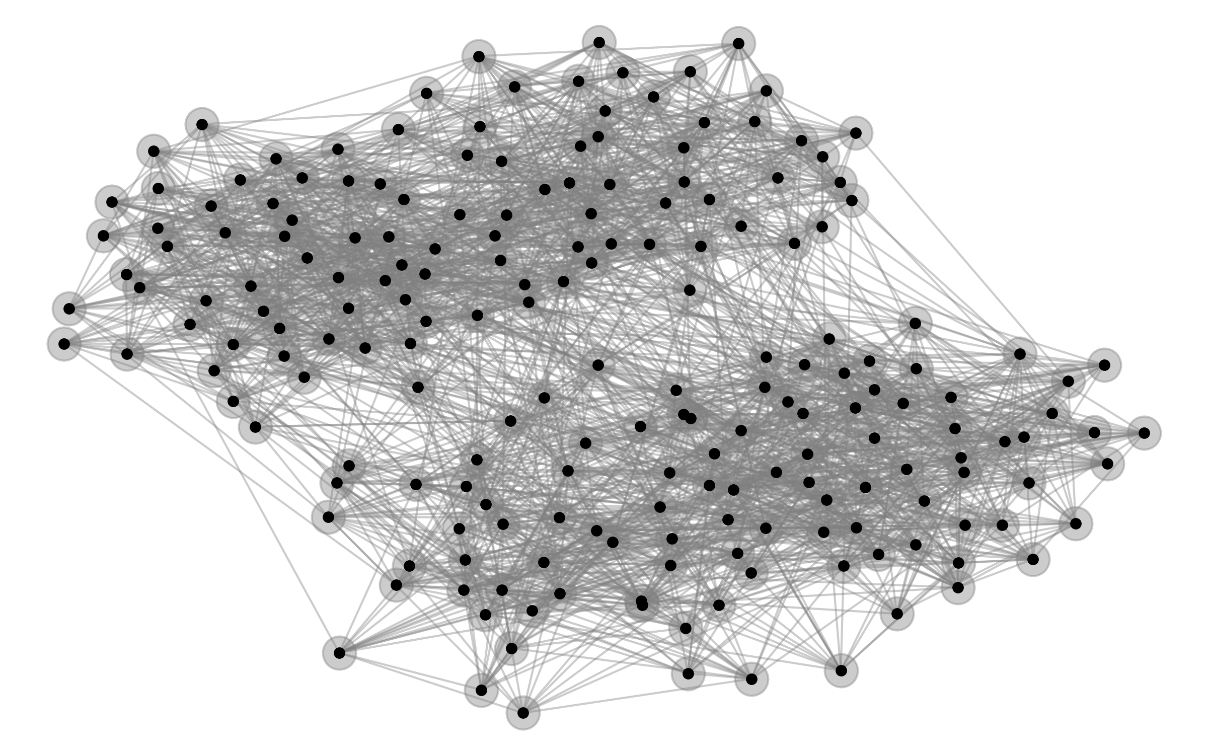
(a)

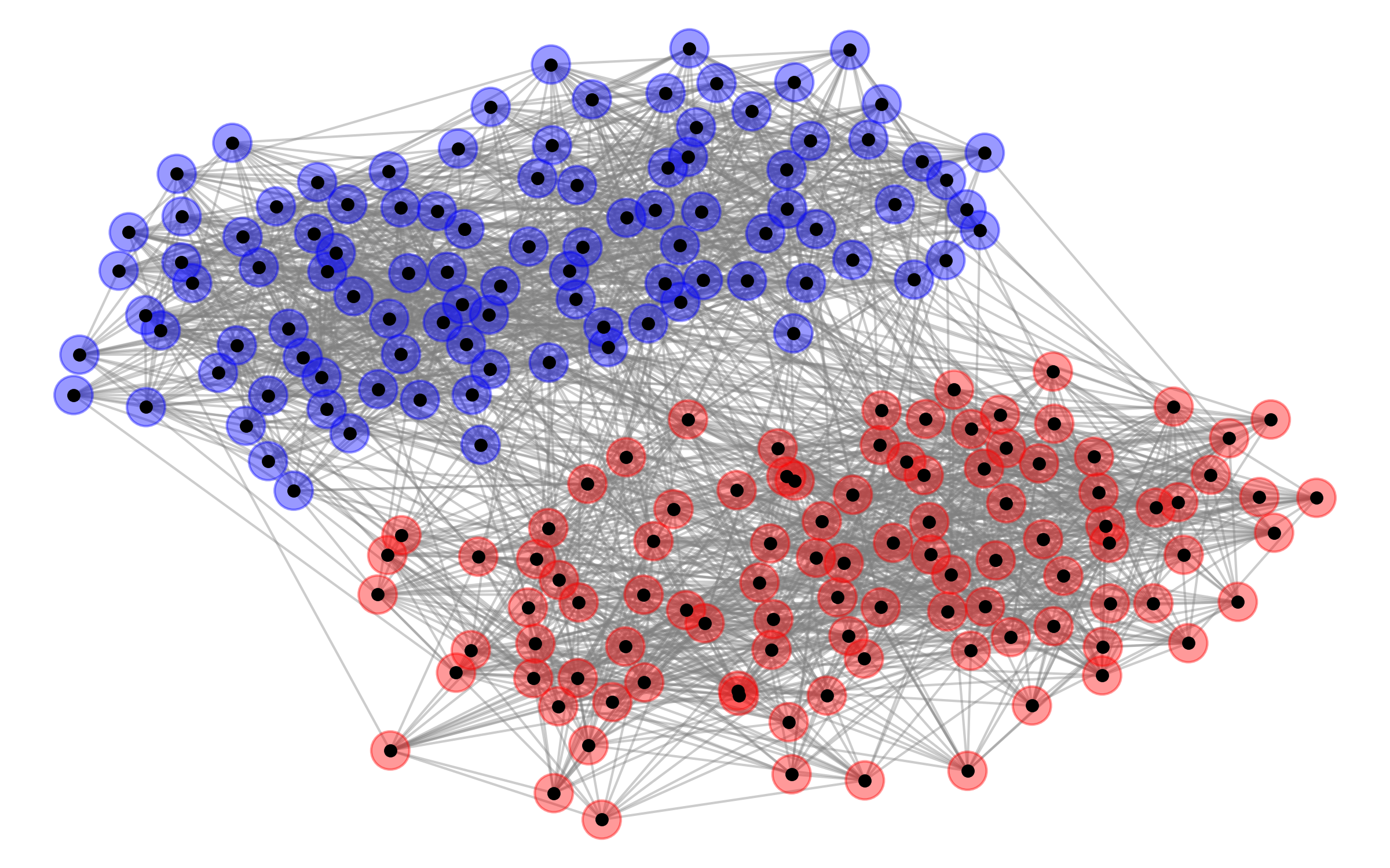
(b)

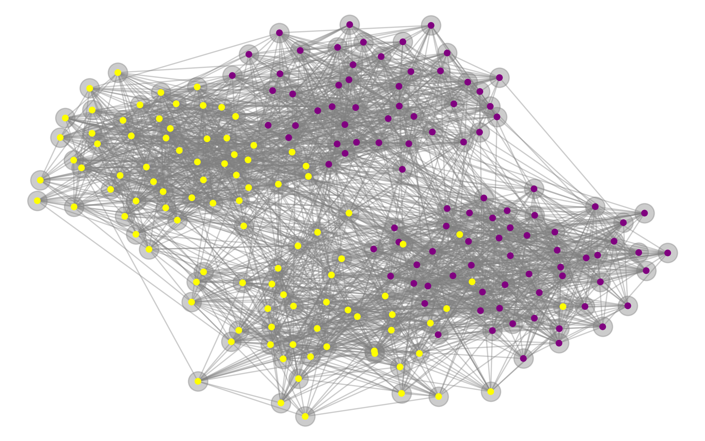
(c)

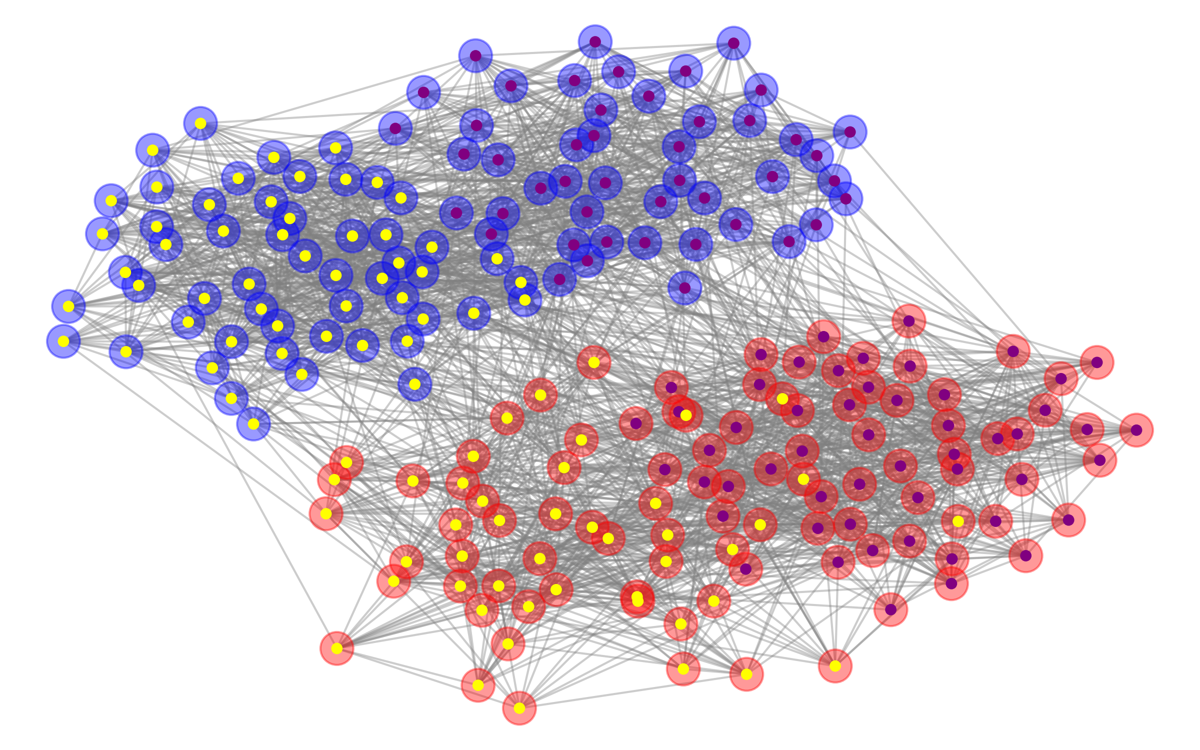
(d)

Figure 1: For each node, (a) both latent variables are unknown, (b) knowing the statistics of the graph, the community latent variable is recovered while the auxiliary latent variable is unknown, (c) the auxiliary latent variable is known while the first one is unknown, (d) knowing the statistics of the graph, the community latent variable is recovered while the auxiliary latent variable is known.

The Chernoff-Hellinger divergence is due to Abbe [24] and is defined for two non-negative vectors $a,b$ of the same dimension:

$$\textup{Div}(a,b) \triangleq\max_{t\in[0,1]}\sum_{i}\big{[}ta_{i}+(1-t)b_{i}-a_{i}^{t}b_{i}^{1-t}\big{]}.$$ (1)

This is a generalization of the Hellinger divergence and the Chernoff divergence [11, 24]. In a manner similar to [11] we present a lemma that bounds a summation of the minimums of Poisson-distributed values.

Lemma 1.

Let $a,b\in\mathbb{R}_{+}^{m}$, with $a\neq b$, and two positive scalars $p,\hat{p}$. For any Poisson multivariate distributions $\mathcal{P}_{a}(d)$ and $\mathcal{P}_{b}(d)$, define

$$I(a,b)\triangleq\sum_{d\in\mathbb{Z}_{+}^{m}}\min\{\mathcal{P}_{a}(d)p,\mathcal{P}_{b}(d)\hat{p}\}.$$

Then

$$I(a,b) \leq\max\{p,\hat{p}\}e^{-\textup{Div}(a,b)},$$

$$I(a,b) \geq\min\{p,\hat{p}\}e^{-\textup{Div}(a,b)}\prod_{i=1}^{m}\frac{1}{e}\big{(}a_{i}^{t^{*}}b_{i}^{1-t^{*}}\big{)}^{-\frac{1}{2}},$$

where $t^{*}$ is the optimal parameter in the definition of Chernoff-Hellinger divergence $\textup{Div}(a,b)$.

Proof.

See Appendix A. ∎

Let $D$ be a random variable vector representing the number of edges that connect the node $v$ to each micro-community. More specifically, ${D^{(i^{\prime},j^{\prime})}}$ is an element of the $D$ indicating the number of edges connecting the node $v$ to the micro-community $(i^{\prime},j^{\prime})$. For each node $v$, the proposed detection tests hypotheses

$$H_{i}:x_{v}=i.$$

If $v$ belongs to micro-community $(i,j)$, then

$${D^{(i^{\prime},j^{\prime})}}\sim\operatorname*{Bin}(nP_{i^{\prime},j^{\prime}},\bar{Q}_{j^{\prime}m_{x}+i^{\prime},jm_{x}+i}).$$

In the regime where $\bar{Q}=Q\frac{\log n}{n}$, the Binomial distribution can be approximated by a Poisson distribution with the same mean, denoted ${\lambda^{(i^{\prime},j^{\prime})}_{i,j}}$. Indeed, using Le Cam’s inequality, the total variation distance between $\operatorname*{Bin}(nP_{i^{\prime},j^{\prime}},\frac{\log n}{n}Q_{j^{\prime}m_{x}+i^{\prime},jm_{x}+i})$ and $\mathcal{P}(P_{i^{\prime},j^{\prime}}Q_{j^{\prime}m_{x}+i^{\prime},jm_{x}+i}\log n)$ asymptotically goes to zero. Then

$${\mathbb{P}}(D=d|H_{i},y_{v}=j)=\prod_{i^{\prime}}\prod_{j^{\prime}}\mathcal{P}_{{\lambda^{(i^{\prime},j^{\prime})}_{i,j}}}({d^{(i^{\prime},j^{\prime})}}),$$

where ${\lambda^{(i^{\prime},j^{\prime})}_{i,j}}=P_{i^{\prime},j^{\prime}}Q_{j^{\prime}m_{x}+i^{\prime},jm_{x}+i}\log n$.

Theorem 1.

Under the two-latent variable stochastic block model, all micro-communities are exactly recovered if and only if

$$\min_{(i,j)\neq(k,l)}\textup{Div}({q^{(i,j)}},{q^{(k,l)}})>1.$$

Proof.

It follows from the exact recovery under the general stochastic bock model or the general overlapping stochastic block model. ∎

Theorem 2.

Under the two-latent variable stochastic block model, when the latent variable $y$ is revealed, exact recovery of $x$ is possible if and only if

$$\gamma_{1}\triangleq\min_{j}\min_{i\neq k}\textup{Div}({q^{(i,j)}},{q^{(k,j)}})>1.$$

Proof.

See Appendix B. ∎

Theorem 3.

Under the two-latent variable stochastic block model, when both latent variables are unknown, exact recovery of $x$ is possible if and only if

$$\gamma_{2}\triangleq\min_{j}\min_{i\neq k}\textup{Div}\big{(}{\tilde{q}^{(i,j)}},{\tilde{q}^{(k,j)}}\big{)}>1.$$

Proof.

See Appendix C. ∎

Now we present the following Lemma which is similar to Lemma 1 and is crucial for the analysis of the censored block model.

Lemma 2.

Let $a,b,\hat{a},\hat{b}\in\mathbb{R}_{+}^{m}$, with $a\neq b$ or $\hat{a}\neq\hat{b}$, and two positive scalars $p,\hat{p}$. For any Poisson multivariate distributions $\mathcal{P}_{a}(d)$, $\mathcal{P}_{b}(d)$, $\mathcal{P}_{\hat{a}}(w)$, and $\mathcal{P}_{\hat{b}}(w)$, define

$$I(a,b,\hat{a},\hat{b})\triangleq\sum_{d,w\in\mathbb{Z}_{+}^{m}}\min\{\mathcal{P}_{a}(d)\mathcal{P}_{\hat{a}}(w)p,\mathcal{P}_{b}(d)\mathcal{P}_{\hat{b}}(w)\hat{p}\}.$$

Then

$$I(a,b,\hat{a},\hat{b})\leq \max\{p,\hat{p}\}e^{-\textup{Div}([a,\hat{a}],[b,\hat{b}])},$$

$$I(a,b,\hat{a},\hat{b})\geq \min\{p,\hat{p}\}e^{-\textup{Div}([a,\hat{a}],[b,\hat{b}])}$$

$$\times\prod_{i}\frac{1}{e^{2}}\big{[}(a_{i}\hat{a}_{i})^{t^{*}}(b_{i}\hat{b}_{i})^{1-t^{*}}\big{]}^{-\frac{1}{2}},$$

where $t^{*}$ is the optimal parameter in the definition of Chernoff-Hellinger divergence $\textup{Div}([a,\hat{a}],[b,\hat{b}])$.

Proof.

See Appendix D. ∎

Let $D$ and $W$ be random vectors representing the positive and negative edges that connect the node $v$ to each micro-community, respectively. More specifically, ${D^{(i^{\prime},j^{\prime})}}$ and ${W^{(i^{\prime},j^{\prime})}}$ are elements of $D$ and $W$ indicating the number of positive and negative edges connecting the node $v$ to the micro-community $(i^{\prime},j^{\prime})$, respectively. For each node $v$, the proposed detection tests hypotheses

$$H_{i}:x_{v}=i.$$

If $v$ belongs to micro-community $(i,j)$, then

$${D^{(i^{\prime},j^{\prime})}}\sim\operatorname*{Bin}(nP_{i^{\prime},j^{\prime}},(\Xi*\bar{Q})_{j^{\prime}m_{x}+i^{\prime},jm_{x}+i}),$$

$${W^{(i^{\prime},j^{\prime})}}\sim\operatorname*{Bin}(nP_{i^{\prime},j^{\prime}},((1-\Xi)*\bar{Q})_{j^{\prime}m_{x}+i^{\prime},jm_{x}+i}).$$

In the regime where $\bar{Q}=Q\frac{\log n}{n}$, the Binomial distribution can be approximated by a Poisson distribution with the same mean. The distributions of $D$ and $W$ can be approximated by multivariate Poisson distributions $\mathcal{P}_{{\lambda_{i,j}}}$ and $\mathcal{P}_{{\hat{\lambda}_{i,j}}}$ with the vector means ${\lambda_{i,j}}$ and ${\hat{\lambda}_{i,j}}$, respectively. Therefore

$${\mathbb{P}}(D=d ,W=w|H_{i},y_{v}=j)$$

$$={\mathbb{P}}(D=d|H_{i},y_{v}=j){\mathbb{P}}(W=w|H_{i},y_{v}=j)$$

$$=\prod_{i^{\prime}}\prod_{j^{\prime}}\mathcal{P}_{{\lambda^{(i^{\prime},j^{\prime})}_{i,j}}}({d^{(i^{\prime},j^{\prime})}})\mathcal{P}_{{\hat{\lambda}^{(i^{\prime},j^{\prime})}_{i,j}}}({w^{(i^{\prime},j^{\prime})}}),$$

where

$${\lambda^{(i^{\prime},j^{\prime})}_{i,j}} =P_{i^{\prime},j^{\prime}}(\Xi*Q)_{j^{\prime}m_{x}+i^{\prime},jm_{x}+i}\log n,$$

$${\hat{\lambda}^{(i^{\prime},j^{\prime})}_{i,j}} =P_{i^{\prime},j^{\prime}}((1-\Xi)*Q)_{j^{\prime}m_{x}+i^{\prime},jm_{x}+i}\log n.$$

Theorem 4.

Under two-latent variable censored block model, all micro-communities are exactly recovered if and only if

$$\min_{(i,j)\neq(k,l)}\textup{Div}\big{(}[{g^{(i,j)}},{h^{(i,j)}}],[{g^{(k,l)}},{h^{(k,l)}}]\big{)}>1.$$

Proof.

See Appendix E. ∎

Theorem 5.

Under the two-latent variable censored block model, when the latent variable $y$ is revealed, exact recovery of $x$ is possible if and only if

$$\gamma_{3}\triangleq\min_{j}\min_{i\neq k}\textup{Div}\big{(}[{g^{(i,j)}},{h^{(i,j)}}],[{g^{(k,j)}},{h^{(k,j)}}]\big{)}>1.$$

Proof.

See Appendix F. ∎

Theorem 6.

Under the two-latent variable censored block model, when both latent variables are unknown, exact recovery of $x$ is possible if and only if

$$\gamma_{4}\triangleq\min_{j}\min_{i\neq k}\textup{Div}\big{(}[{\tilde{g}^{(i,j)}},{\tilde{h}^{(i,j)}}],[{\tilde{g}^{(k,j)}},{\tilde{h}^{(k,j)}}]\big{)}>1.$$

Proof.

See Appendix G. ∎

Corollary 1.

Assume $x$ and $y$ are unknown latent variables for all nodes. We randomly reveal the latent variable $y$ for $(1-\epsilon)n$ nodes, where $\epsilon\in(0,1)$. This is equivalent to erasing the latent variable $y$ which is a known latent variable from a node with erasure probability $\epsilon$. Define

$$\beta_{1}\triangleq-\lim_{n\rightarrow\infty}\frac{\log(1-\epsilon)}{\log n},\quad\beta_{2}\triangleq-\lim_{n\rightarrow\infty}\frac{\log\epsilon}{\log n}.$$

• Under the two-latent variable stochastic block model exact recovery is asymptotically possible for latent variable $x$ if and only if

  $$\min\big{(}\gamma_{1}+\beta_{1},\gamma_{2}+\beta_{2}\big{)}>1.$$

• Under the two-latent variable censored block model exact recovery is asymptotically possible for latent variable $x$ if and only if

  $$\min\big{(}\gamma_{3}+\beta_{1},\gamma_{4}+\beta_{2}\big{)}>1.$$

The results of this part generalize to $M$ latent variables without difficulty.

Remark 2.

To prove the “if” part of all theorems in Section III, a partial recovery algorithm is required before applying a MAP estimator. For that purpose, the partial recovery algorithm in [11] is adopted and modified to match the scenarios in this paper. Please see Appendix I.

IV Semidefinite Programming Results

This section describes a semidefinite programming algorithm for recovering the desired latent variable. The main results of this part are represented in the context of two scenarios, where the latent variable $x$ is unknown and the latent variable $y$ is either known or unknown (for all nodes in the graph). We consider $x,y\in\{\pm 1\}^{n}$ such that $x^{T}\mathbf{1}=0$. Thus, the latent variable $x$ represents two equal-sized communities. The sample size of the latent variable $y$, represented by $\rho\triangleq\frac{1}{n}|\{v\in[n]:y_{v}=1\}|$, is an unknown quantity.

IV-A Two-latent variable stochastic block model

We highlight the specifics of a two-latent variable stochastic block model for the purposes of upcoming calculations. The probability of an edge drawn between two nodes $v,u$ is characterized by four constants, $q_{0},q_{1},q_{2},q_{3}$ such that:

$$A_{ij}\sim\begin{cases}\operatorname*{Bern}(q_{0}\frac{\log n}{n})&\text{if}\quad x_{v}=x_{u},y_{v}=y_{u}\\ \operatorname*{Bern}(q_{1}\frac{\log n}{n})&\text{if}\quad x_{v}\neq x_{u},y_{v}=y_{u}\\ \operatorname*{Bern}(q_{2}\frac{\log n}{n})&\text{if}\quad x_{v}=x_{u},y_{v}\neq y_{u}\\ \operatorname*{Bern}(q_{3}\frac{\log n}{n})&\text{if}\quad x_{v}\neq x_{u},y_{v}\neq y_{u}\end{cases}.$$

The corresponding matrix $Q$, as defined earlier, in this case will be:

$$Q=\begin{bmatrix}q_{0}&q_{1}&q_{2}&q_{3}\\ q_{1}&q_{0}&q_{3}&q_{2}\\ q_{2}&q_{3}&q_{0}&q_{1}\\ q_{3}&q_{2}&q_{1}&q_{0}\end{bmatrix}.$$ (2)

IV-A1 Recovering $x$ when $y$ is known

In the first scenario, given an observation of the graph $A$ and $y$ which corresponds to the observed graph, the latent variable $x_{v}$ is recovered exactly for each node $v\in[n]$. In this part, $y$ is considered as an observation which helps the estimator to recover the desired latent variable $x$. Let $W\triangleq yy^{T}$ and $B\triangleq W*A$. Since $x$ is chosen uniformly over $\{x\in\{\pm 1\}^{n}:x^{T}\mathbf{1}=0\}$, the maximum likelihood estimator gives the optimal solution. For this configuration, the log-likelihood is

$$\log{\mathbb{P}}(A|x,y)=\frac{T_{1}}{8}x^{T}Bx+\frac{T_{2}}{8}x^{T}Ax+c,$$

where $T_{1}\triangleq\log(\frac{q_{0}q_{3}}{q_{2}q_{1}})$ and $T_{2}\triangleq\log(\frac{q_{0}q_{2}}{q_{1}q_{3}})$, as $n\rightarrow\infty$ and $c$ is a constant. Considering the constraints, the maximum likelihood estimator is,

$$\hat{x}= \underset{x}{\arg\max}~{}T_{1}x^{T}Bx+T_{2}x^{T}Ax$$

$$\text{subject to}\quad x_{i}\in\{\pm 1\},\quad i\in[n]$$

$$\quad\quad\quad\quad\quad x^{T}\mathbf{1}=0,$$ (3)

which is a non-convex optimization problem. Let $Z=xx^{T}$. Reorganizing (IV-A1),

$$\hat{Z}= \underset{Z}{\arg\max}~{}\langle Z,T_{1}B+T_{2}A\rangle$$

$$\text{subject to}\quad Z=xx^{T}$$

$$\quad\quad\quad\quad\quad Z_{ii}=1,\quad i\in[n]$$

$$\quad\quad\quad\quad\quad\langle Z,\mathbf{J}\rangle=0.$$ (4)

By relaxing the rank-one constraint on $Z$, we obtain the following semidefinite programming relaxation of (IV-A1):

$$\hat{Z}= \underset{Z}{\arg\max}~{}\langle Z,T_{1}B+T_{2}A\rangle$$

$$\text{subject to}\quad Z\succeq 0$$

$$\quad\quad\quad\quad\quad Z_{ii}=1,\quad i\in[n]$$

$$\quad\quad\quad\quad\quad\langle Z,\mathbf{J}\rangle=0.$$ (5)

For convenience define

$$\eta_{1}(\mathbf{q},\rho)\triangleq\frac{\rho}{2}(\sqrt{q_{0}}-\sqrt{q_{1}})^{2}+\frac{1-\rho}{2}(\sqrt{q_{2}}-\sqrt{q_{3}})^{2},$$

where $\mathbf{q}\triangleq[q_{0},q_{1},q_{2},q_{3}]$.

Theorem 7.

Under the two-latent variable stochastic block model with binary alphabet where the latent variable $y$ has been revealed, if

$$\begin{cases}\eta_{1}(\mathbf{q},\rho)>1&\text{when}\quad\rho\leq 0.5\\ \eta_{1}(\mathbf{q},1-\rho)>1&\text{when}\quad\rho>0.5\end{cases}$$

then the semidefinite programming estimator is asymptotically optimal, i.e., ${\mathbb{P}}(\hat{Z}=Z^{*})\geq 1-o(1)$. Also, if

$$\begin{cases}\eta_{1}(\mathbf{q},\rho)<1&\text{when}\quad\rho\leq 0.5\\ \eta_{1}(\mathbf{q},1-\rho)<1&\text{when}\quad\rho>0.5\end{cases}$$

then for any sequence of estimators $\hat{Z}_{n}$, ${\mathbb{P}}(\hat{Z}_{n}=Z^{*})\rightarrow 0$.

Proof.

See Appendix H. ∎

IV-A2 Recovering $x$ when $y$ is unknown

Given an observation of the graph $A$, the aim is to exactly recover $x$ while both latent variables $x$ and $y$ are unknown latent variables. It is assumed that the estimator does not know anything about the auxiliary latent variable $y$, which its prior distribution is uniform over $\{y:y\in\{\pm 1\}^{n}\}$. Notice that $x$ is drawn uniformly from $\{x\in\{\pm 1\}^{n}:x^{T}\mathbf{1}=0\}$. The log-likelihood of $A$ given $x$ and $y$ is

$$\log{\mathbb{P}}(A|x,y)= \frac{T_{1}}{8}y^{T}(A*xx^{T})y+\frac{T_{2}}{8}x^{T}Ax+\frac{T_{3}}{8}y^{T}Ay+c,$$

where $T_{1}\triangleq\log(\frac{q_{0}q_{3}}{q_{2}q_{1}})$, $T_{2}\triangleq\log(\frac{q_{0}q_{2}}{q_{1}q_{3}})$, and $T_{3}\triangleq\log(\frac{q_{0}q_{1}}{q_{2}q_{3}})$, as $n\rightarrow\infty$ and $c$ is a constant. Then

$$\log {\mathbb{P}}(A|x)\propto\log\sum_{\mathcal{Y}}{\mathbb{P}}(A|x,y)$$

$$\propto \log\sum_{\mathcal{Y}}e^{\frac{T_{1}}{T_{3}}y^{T}(A*xx^{T})y+\frac{T_{2}}{T_{3}}x^{T}Ax+y^{T}Ay}$$

$$= \frac{T_{1}+T_{2}}{T_{3}}x^{T}Ax+\sum_{i}\sum_{j}A_{ij}$$

$$+\log\sum_{\mathcal{Y}}e^{\frac{T_{1}}{T_{3}}y^{T}(A*xx^{T})y+y^{T}Ay-\frac{T_{1}}{T_{3}}x^{T}Ax-\sum_{i}\sum_{j}A_{ij}}.$$

Applying the log-sum-exp approximation, the maximum likelihood estimator is

$$\hat{x}= \underset{x}{\arg\max}~{}x^{T}Ax$$

$$\text{subject to}\quad x_{i}\in\{\pm 1\},\quad i\in[n]$$

$$\quad\quad\quad\quad\quad x^{T}\mathbf{1}=0,$$ (6)

that is a non-convex optimization problem. Let $Z=xx^{T}$. Reorganizing (IV-A2) yields

$$\hat{Z}= \underset{Z}{\arg\max}~{}\langle Z,A\rangle$$

$$\text{subject to}\quad Z=xx^{T}$$

$$\quad\quad\quad\quad\quad Z_{ii}=1,\quad i\in[n]$$

$$\quad\quad\quad\quad\quad\langle Z,\mathbf{J}\rangle=0.$$ (7)

Relaxing the rank-one constraint on $Z$, we obtain the following semidefinite programming relaxation of (IV-A2):

$$\hat{Z}= \underset{Z}{\arg\max}~{}\langle Z,A\rangle$$

$$\text{subject to}\quad Z\succeq 0$$

$$\quad\quad\quad\quad\quad Z_{ii}=1,\quad i\in[n]$$

$$\quad\quad\quad\quad\quad\langle Z,\mathbf{J}\rangle=0.$$ (8)

For convenience define

$$\eta_{2} (\mathbf{q},\rho)\triangleq\frac{1}{2}\bigg{(}\sqrt{q_{0}\rho+q_{2}(1-\rho)}-\sqrt{q_{1}\rho+q_{3}(1-\rho)}\bigg{)}^{2}.$$

Theorem 8.

Under the two-latent variable stochastic block model with binary alphabet, if

$$\min{\{\eta_{2}(\mathbf{q},\rho),\eta_{2}(\mathbf{q},1-\rho)\}}>1,$$

then the semidefinite programming estimator is asymptotically optimal, i.e., ${\mathbb{P}}(\hat{Z}=Z^{*})\geq 1-o(1)$. Also, if

$$\min{\{\eta_{2}(\mathbf{q},\rho),\eta_{2}(\mathbf{q},1-\rho)\}}<1,$$

then for any sequence of estimators $\hat{Z}_{n}$, ${\mathbb{P}}(\hat{Z}_{n}=Z^{*})\rightarrow 0$.

Proof.

See Appendix J. ∎

Remark 3.

The results of Theorems 7 and 8 are consistent with Theorems 2 and 3, respectively.

Remark 4.

The constraint $x^{T}\mathbf{1}=0$ that has been considered for this part results in a well-defined phase transition threshold for exact recovery of latent variable $x$. In general, $x$ may be a random variable which is drawn uniformly from $\{x\in\{\pm 1\}^{n}:x^{T}\mathbf{1}=(2\rho_{x}-1)n\}$, where $\rho_{x}\triangleq\frac{1}{n}|\{v\in[n]:x_{v}=1\}|$. Then $x^{T}\mathbf{1}=0$ is substituted by $x^{T}\mathbf{1}=(2\rho_{x}-1)n$ in semidefinite programming relaxations (IV-A1) and (IV-A2). Also, due to the robustness of semidefinite programming, an approximation of $\rho_{x}$ can be replaced for recovering the latent variable $x$. Investigating the constraint $x^{T}\mathbf{1}=(2\rho_{x}-1)n$ and the robustness of semidefinite programming are beyond the scope of this paper.

IV-B Two-latent variable censored block model

We highlight the specifics of a two-latent variable censored block model for the purposes of upcoming calculations. Let $P(k;q_{0},\xi)$ be a discrete probability density function with parameters $q_{0}>0$ and $\xi\in[0,1]$ as,

$$P(k;q_{0},\xi)\triangleq \xi q_{0}\frac{\log n}{n}\delta[k-1]+(1-\xi)q_{0}\frac{\log n}{n}\delta[k+1]$$

$$+\Big{(}1-q_{0}\frac{\log n}{n}\Big{)}\delta[k],$$

where $\delta$ is Dirac delta function. The probability of an edge drawn between two nodes $v,u$ is characterized by constants $q_{0},q_{1},q_{2},q_{3}$ and $\xi$ such that:

$$A_{ij}\sim\begin{cases}P(k;q_{0},1-\xi)&\text{if}\quad x_{v}=x_{u},y_{v}=y_{u}\\ P(k;q_{1},\xi)&\text{if}\quad x_{v}\neq x_{u},y_{v}=y_{u}\\ P(k;q_{2},\xi)&\text{if}\quad x_{v}=x_{u},y_{v}\neq y_{u}\\ P(k;q_{3},\xi)&\text{if}\quad x_{v}\neq x_{u},y_{v}\neq y_{u}\end{cases}.$$

The corresponding matrix $Q$, as defined earlier, is the same as (2). Also, in this case, the corresponding matrix $\Xi$ will be:

$$\Xi=\begin{bmatrix}(1-\xi)&\xi&\xi&\xi\\ \xi&(1-\xi)&\xi&\xi\\ \xi&\xi&(1-\xi)&\xi\\ \xi&\xi&\xi&(1-\xi)\end{bmatrix}.$$ (9)

IV-B1 Recovering $x$ when $y$ is known

Given an observation of the graph $A$ and $y$ which corresponds to the observed graph, the latent variable $x_{v}$ is recovered exactly for each node $v\in[n]$. In this part, $y$ is considered as an observation which helps the estimator to recover the desired latent variable $x$. Let

$$R\triangleq TA+T(A*W)+T_{1}(A*A*W)+T_{2}(A*A),$$

where $T\triangleq\log\big{(}\frac{1-\xi}{\xi}\big{)}$ and $W\triangleq yy^{T}$. Since $x$ is chosen uniformly over $\{x\in\{\pm 1\}^{n}:x^{T}\mathbf{1}=0\}$, the maximum likelihood estimator gives the optimal solution. Similar to Section IV-A1, it can be shown that the semidefinite programming relaxation of maximum likelihood estimator for this configuration is

$$\hat{Z}= \underset{Z}{\arg\max}~{}\langle Z,R\rangle$$

$$\text{subject to}\quad Z\succeq 0$$

$$\quad\quad\quad\quad\quad Z_{ii}=1,\quad i\in[n]$$

$$\quad\quad\quad\quad\quad\langle Z,\mathbf{J}\rangle=0.$$ (10)

For convenience define

$$\mathbf{g} \triangleq[(1-\xi)q_{0},\xi q_{1},\xi q_{2},\xi q_{3}],$$

$$\mathbf{h} \triangleq[\xi q_{0},(1-\xi)q_{1},(1-\xi)q_{2},(1-\xi)q_{3}].$$

Theorem 9.

Under the two-latent variable censored block model with binary alphabet where the latent variable $y$ has been revealed, if

$$\begin{cases}\eta_{1}(\mathbf{g},\rho)+\eta_{1}(\mathbf{h},\rho)>1&\text{when}\quad\rho\leq 0.5\\ \eta_{1}(\mathbf{g},1-\rho)+\eta_{1}(\mathbf{h},1-\rho)>1&\text{when}\quad\rho>0.5\end{cases}$$

then the semidefinite programming estimator is asymptotically optimal, i.e., ${\mathbb{P}}(\hat{Z}=Z^{*})\geq 1-o(1)$. Also, if

$$\begin{cases}\eta_{1}(\mathbf{g},\rho)+\eta_{1}(\mathbf{h},\rho)<1&\text{when}\quad\rho\leq 0.5\\ \eta_{1}(\mathbf{g},1-\rho)+\eta_{1}(\mathbf{h},1-\rho)<1&\text{when}\quad\rho>0.5\end{cases}$$

then for any sequence of estimators $\hat{Z}_{n}$, ${\mathbb{P}}(\hat{Z}_{n}=Z^{*})\rightarrow 0$.

Proof.

See Appendix K. ∎

IV-B2 Recovering $x$ when $y$ is unknown

Given an observation of the graph $A$, the aim is to exactly recover $x$ while both latent variables $x$ and $y$ are unknown. It is assumed that the estimator does not know anything about the auxiliary latent variable $y$, which its prior distribution is uniform over $\{y:y\in\{\pm 1\}^{n}\}$. Notice that $x$ is drawn uniformly from $\{x\in\{\pm 1\}^{n}:x^{T}\mathbf{1}=0\}$. Similar to Section IV-A2, it can be shown that for this configuration the semidefinite programming relaxation of the maximum likelihood estimator is

$$\hat{Z}= \underset{Z}{\arg\max}~{}\langle Z,TA+T_{2}(A*A)\rangle$$

$$\text{subject to}\quad Z\succeq 0$$

$$\quad\quad\quad\quad\quad Z_{ii}=1,\quad i\in[n]$$

$$\quad\quad\quad\quad\quad\langle Z,\mathbf{J}\rangle=0.$$ (11)

Theorem 10.

Under the two-latent variable censored block model with binary alphabet, if

$$\min\big{\{}\eta_{2}(\mathbf{g},\rho)+\eta_{2}(\mathbf{h},\rho),\eta_{2}(\mathbf{g},1-\rho)+\eta_{2}(\mathbf{h},1-\rho)\big{\}}>1,$$

then the semidefinite programming estimator is asymptotically optimal, i.e., ${\mathbb{P}}(\hat{Z}=Z^{*})\geq 1-o(1)$. Also, if

$$\min\big{\{}\eta_{2}(\mathbf{g},\rho)+\eta_{2}(\mathbf{h},\rho),\eta_{2}(\mathbf{g},1-\rho)+\eta_{2}(\mathbf{h},1-\rho)\big{\}}<1,$$

then for any sequence of estimators $\hat{Z}_{n}$, ${\mathbb{P}}(\hat{Z}_{n}=Z^{*})\rightarrow 0$.

Proof.

See Appendix L. ∎

Remark 5.

The results of Theorems 9 and 10 are consistent with Theorems 5 and 6, respectively.

V Discussion & Numerical Results

It is illuminating to review the flow of the development of the achievability results througout this paper:

1. Calculate the Lagrangian of the corresponding optimization

2. Extract the dual optimal solution based on the Lagrange multipliers

3. Show that $\hat{Z}=Z^{*}$ is primal optimal solution

4. Show that $\hat{Z}=Z^{*}$ is unique

5. Extract the conditions under which the dual optimal solution holds

The converses follow the following sequence:

1. Extract the maximum likelihood estimator

2. Extract the conditions under which the maximum likelihood estimator fails

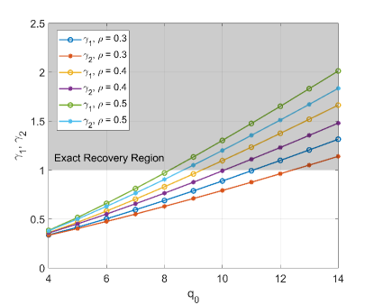
Figure 2: Exact recovery region of $x$ in the context of Eq. (2), with $q_{2}=3,q_{1}=q_{3}=1$.

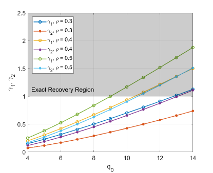
Figure 3: Exact recovery region of $x$ in the context of Eq. (2), with $q_{1}=q_{2}=q_{3}=1$.

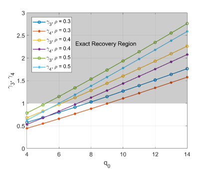
Figure 4: Exact recovery region of $x$ in the context of Eq. (2) and Eq. (9), with $\xi=0.1$, $q_{2}=3$, and $q_{1}=q_{3}=1$.

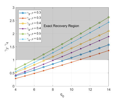
Figure 5: Exact recovery region of $x$ in the context of Eq. (2) and Eq. (9), with $\xi=0.1$, and $q_{1}=q_{2}=q_{3}=1$.

To give a pictorial view of some results of the paper, we plot some results in the context of the two-latent variable stochastic block model represented by (2) and two-latent variable censored block model represented by (2) and (9). For ease of notation, we define

$$\gamma_{1}\triangleq\min\{\eta_{1}(\mathbf{q},\rho),\eta_{1}(\mathbf{q},1-\rho)\},$$

$$\gamma_{2}\triangleq\min\{\eta_{2}(\mathbf{q},\rho),\eta_{2}(\mathbf{q},1-\rho)\},$$

$$\gamma_{3}\triangleq\min\{\eta_{1}(\mathbf{g},\rho)+\eta_{1}(\mathbf{h},\rho),\eta_{1}(\mathbf{g},1-\rho)+\eta_{1}(\mathbf{h},1-\rho)\},$$

$$\gamma_{4}\triangleq\min\{\eta_{2}(\mathbf{g},\rho)+\eta_{2}(\mathbf{h},\rho),\eta_{2}(\mathbf{g},1-\rho)+\eta_{2}(\mathbf{h},1-\rho)\}.$$

For the two-latent variable stochastic block model, Figures 2 and  3 show the exact recovery region for recovering the latent variable $x$ when the secondary latent variable $y$ is either known or unknown. The curves in these figures are based on the obtained results in Theorem 7 and Theorem 8. These figures encompass several curves plotted for different values of $q_{0}$, $q_{1}$, $q_{2}$, $q_{3}$ in (2), and $\rho$. At each figure, we consider fixed values for $q_{1}$, $q_{2}$, $q_{3}$ and vary the values of $q_{0}$ and $\rho$. A comparison between the curves in Figures 2 and 3 clarifies the role of the revealed latent variable $y$ for recovering the desired latent variable $x$.

For the two-latent variable censored block model, Figures 4 and  5 show the exact recovery region for recovering the latent variable $x$ when the secondary latent variable $y$ is either known or unknown. The curves in these figures are based on the obtained results in Theorem 9 and Theorem 10. These figures consist of several curves plotted for different values of $q_{0}$, $q_{1}$, $q_{2}$, $q_{3}$ in (2) and $\rho$, while $\xi=0.1$ in (9). At each figure, we consider fixed values for $\xi$, $q_{1}$, $q_{2}$, $q_{3}$ and vary the values of $q_{0}$ and $\rho$. A comparison between the curves in Figures 4 and 5 clarifies the role of the revealed latent variable $y$ for recovering the desired latent variable $x$.

To gain an understanding of the scope of our asymptotic results, under the conditions of Figures 2 and 4, we performed several simulations on $10^{4}$ graph realizations with various graph sizes obtained from the proposed models in Section II. The obtained average error probability (AEP) is around $10^{-5}$ in the regimes just inside the region of exact recovery, and around $10^{-2}$ in the regimes just outside the region of exact recovery. The details of these simulations are represented in Tables I and II. At each simulation, we consider fixed values for $q_{1}$, $q_{2}$, $q_{3}$ and vary the values of $q_{0}$, $\rho$, and $n$.

$y$	$n$	BSBM		BCBM
		$q_{0}$	AEP	$q_{0}$	$\xi$	AEP
Known	100	7	$3.8\times 10^{-2}$	4	0.1	$6.7\times 10^{-2}$
Known	200	7	$2.4\times 10^{-2}$	4	0.1	$4.9\times 10^{-2}$
Known	300	7	$1.9\times 10^{-2}$	4	0.1	$3.6\times 10^{-2}$
Known	400	7	$1.5\times 10^{-2}$	4	0.1	$2.5\times 10^{-2}$
Known	500	7	$1.1\times 10^{-2}$	4	0.1	$1.6\times 10^{-2}$
Known	100	9	$8.1\times 10^{-5}$	6	0.1	$4.6\times 10^{-5}$
Known	200	9	$5.9\times 10^{-5}$	6	0.1	$3.2\times 10^{-5}$
Known	300	9	$4.2\times 10^{-5}$	6	0.1	$2.4\times 10^{-5}$
Known	400	9	$2.8\times 10^{-5}$	6	0.1	$1.7\times 10^{-5}$
Known	500	9	$1.8\times 10^{-5}$	6	0.1	$1.2\times 10^{-5}$
Unknown	100	8	$5.7\times 10^{-2}$	5	0.1	$5.6\times 10^{-2}$
Unknown	200	8	$4.1\times 10^{-2}$	5	0.1	$3.9\times 10^{-2}$
Unknown	300	8	$2.7\times 10^{-2}$	5	0.1	$2.5\times 10^{-2}$
Unknown	400	8	$1.8\times 10^{-2}$	5	0.1	$1.6\times 10^{-2}$
Unknown	500	8	$1.3\times 10^{-2}$	5	0.1	$1.1\times 10^{-2}$
Unknown	100	10	$6.2\times 10^{-5}$	7	0.1	$6.3\times 10^{-5}$
Unknown	200	10	$4.4\times 10^{-5}$	7	0.1	$4.0\times 10^{-5}$
Unknown	300	10	$3.3\times 10^{-5}$	7	0.1	$2.3\times 10^{-5}$
Unknown	400	10	$2.3\times 10^{-5}$	7	0.1	$1.7\times 10^{-5}$
Unknown	500	10	$1.4\times 10^{-5}$	7	0.1	$1.3\times 10^{-5}$

TABLE I: Semidefinite programming optimization of (8) and (10), with $q_{2}=3,q_{1}=q_{3}=1$, and $\rho=0.5$.

$y$	$n$	BSBM		BCBM
		$q_{0}$	AEP	$q_{0}$	$\xi$	AEP
Known	100	10	$7.6\times 10^{-2}$	7	0.1	$4.1\times 10^{-2}$
Known	200	10	$5.1\times 10^{-2}$	7	0.1	$3.1\times 10^{-2}$
Known	300	10	$3.0\times 10^{-2}$	7	0.1	$2.3\times 10^{-2}$
Known	400	10	$2.1\times 10^{-2}$	7	0.1	$1.8\times 10^{-2}$
Known	500	10	$1.3\times 10^{-2}$	7	0.1	$1.3\times 10^{-2}$
Known	100	12	$6.7\times 10^{-5}$	9	0.1	$3.9\times 10^{-5}$
Known	200	12	$5.1\times 10^{-5}$	9	0.1	$2.5\times 10^{-5}$
Known	300	12	$3.6\times 10^{-5}$	9	0.1	$1.8\times 10^{-5}$
Known	400	12	$2.5\times 10^{-5}$	9	0.1	$1.2\times 10^{-5}$
Known	500	12	$1.6\times 10^{-5}$	9	0.1	$1.0\times 10^{-5}$
Unknown	100	11	$4.3\times 10^{-2}$	8	0.1	$4.2\times 10^{-2}$
Unknown	200	11	$3.3\times 10^{-2}$	8	0.1	$2.9\times 10^{-2}$
Unknown	300	11	$2.4\times 10^{-2}$	8	0.1	$2.0\times 10^{-2}$
Unknown	400	11	$1.7\times 10^{-2}$	8	0.1	$1.3\times 10^{-2}$
Unknown	500	11	$1.2\times 10^{-2}$	8	0.1	$1.0\times 10^{-2}$
Unknown	100	13	$4.2\times 10^{-5}$	10	0.1	$4.8\times 10^{-5}$
Unknown	200	13	$2.6\times 10^{-5}$	10	0.1	$3.3\times 10^{-5}$
Unknown	300	13	$1.7\times 10^{-5}$	10	0.1	$2.2\times 10^{-5}$
Unknown	400	13	$1.3\times 10^{-5}$	10	0.1	$1.5\times 10^{-5}$
Unknown	500	13	$1.1\times 10^{-5}$	10	0.1	$1.0\times 10^{-5}$

TABLE II: Semidefinite programming optimization of (8) and (10), with $q_{2}=3,q_{1}=q_{3}=1$, and $\rho=0.3$.

VI Conclusion

This paper presents and analyzes a new generalization of the stochastic and censored block models in which, in addition to the latent variable representing community labels, there exists another (secondary) latent variables that are not part of community detection. These secondary latent variables may be known, unknown, or partially known. This model represents community detection problems where the community labels alone does not explain all the dependencies between the graph edges.

We investigate the exact recovery threshold for these models under maximum likelihood detection, and also analyze a semidefinite programming algorithm for recovering the desired latent variable under the two-latent variable stochastic block model and the two-latent variable censored block model for both scenarios.

Appendix A Proof of Lemma 1

Define

$$f_{1}(t) \triangleq\prod_{i=1}^{m}\bigg{(}\frac{b_{i}}{a_{i}}\bigg{)}^{(t-1)d_{i}}e^{(t-1)(a_{i}-b_{i})},$$

$$f_{2}(t) \triangleq\prod_{i=1}^{m}\bigg{(}\frac{b_{i}}{a_{i}}\bigg{)}^{td_{i}}e^{t(a_{i}-b_{i})}.$$

For any $t\in[0,1]$,

$$\sum_{d\in\mathbb{Z}_{+}^{m}} \min\{\mathcal{P}_{a}(d)p,\mathcal{P}_{b}(d)\hat{p}\}$$

$$\leq \max\{p,\hat{p}\}\sum_{d\in{\mathbb{Z}_{+}^{m}}}\min\{\mathcal{P}_{a}(d),\mathcal{P}_{b}(d)\}$$

$$= \max\{p,\hat{p}\}\exp\bigg{(}-\sum_{i}\big{[}ta_{i}+(1-t)b_{i}-a_{i}^{t}b_{i}^{1-t}\big{]}\bigg{)}$$

$$\times\sum_{d\in\mathbb{Z}_{+}^{m}}\prod_{i}\frac{(a_{i}^{t}b_{i}^{1-t})^{d_{i}}}{d_{i}!}e^{-a_{i}^{t}b_{i}^{1-t}}\min\{f_{1}(t),f_{2}(t)\}.$$

Both $f_{1}(t)$ and $f_{2}(t)$ are monotonic and $\frac{f_{2}(t)}{f_{1}(t)}$ is a positive constant (does not depend on $t$), thus $\min\{f_{1},f_{2}\}$ is also monotonic in $t$. Since $f_{1}(1)=f_{2}(0)=1$, for all $t$ we have:

$$\min\{f_{1}(t),f_{2}(t)\}\leq 1.$$

Notice that

$$\sum_{d\in\mathbb{Z}_{+}^{m}}\prod_{i}\frac{(a_{i}^{t}b_{i}^{1-t})^{d_{i}}}{d_{i}!}e^{-a_{i}^{t}b_{i}^{1-t}}=1.$$

Then

$$I(a,b)\leq\max\{p,\hat{p}\}e^{-\sum_{i=1}^{m}\big{[}ta_{i}+(1-t)b_{i}-a_{i}^{t}b_{i}^{1-t}\big{]}}.$$ (12)

For the value of $t$ that maximizes the right-hand side of inequality (12), we have

$$\sum_{d\in\mathbb{Z}_{+}^{m}}\min\{\mathcal{P}_{a}(d)p,\mathcal{P}_{b}(d)\hat{p}\} \leq\max\{p,\hat{p}\}e^{-\textup{Div}(a,b)}.$$

Notice that $t^{*}$ satisfies

$$\prod_{i=1}^{m}\bigg{(}\frac{b_{i}}{a_{i}}\bigg{)}^{a_{i}^{t^{*}}b_{i}^{1-t^{*}}}e^{a_{i}-b_{i}}=1.$$

Then at the optimal $t^{*}$,

$$\sum_{d\in\mathbb{Z}_{+}^{m}} \min\{\mathcal{P}_{a}(d)p,\mathcal{P}_{b}(d)\hat{p}\}$$

$$\geq \min\{p,\hat{p}\}\sum_{d\in\mathbb{Z}_{+}^{m}}\min\{\mathcal{P}_{a}(d),\mathcal{P}_{b}(d)\}$$

$$\overset{(a)}{\geq} \min\{p,\hat{p}\}e^{-\textup{Div}(a,b)}\prod_{i}\frac{(a_{i}^{t^{*}}b_{i}^{1-t^{*}})^{a_{i}^{t^{*}}b_{i}^{1-t^{*}}}}{a_{i}^{t^{*}}b_{i}^{1-t^{*}}!}e^{-a_{i}^{t^{*}}b_{i}^{1-t^{*}}}$$

$$\overset{(b)}{\geq} \min\{p,\hat{p}\}e^{-\textup{Div}(a,b)}\prod_{i}\frac{1}{e}\big{(}a_{i}^{t^{*}}b_{i}^{1-t^{*}}\big{)}^{-\frac{1}{2}},$$

where $(a)$ holds because

$$\sum_{d\in\mathbb{Z}_{+}^{m}}\min\{\mathcal{P}_{a}(d),\mathcal{P}_{b}(d)\}\geq\min\{\mathcal{P}_{a}(d^{*}),\mathcal{P}_{b}(d^{*})\},$$

where $d^{*}$ is defined by $d_{i}^{*}\triangleq a_{i}^{t^{*}}b_{i}^{1-t^{*}}$, and $(b)$ is due to Stirling’s approximation $n!\leq n^{n+\frac{1}{2}}e^{-n+1}$ for any $n\geq 1$.

Appendix B Proof of Theorem 2

We aim to recover $x_{v}$ when $y_{v}$ is known. Given a realization of $D$ and $y_{v}$, our goal is to minimize the error probability by selecting the most likely hypothesis, i.e.,

$$\operatorname*{argmax}_{i}{\mathbb{P}}\{H_{i}|D=d,y_{v}\},$$

or equivalently, since $d,y_{v}$ are known observations,

$$\operatorname*{argmax}_{i}P(d|H_{i},y_{v}){\mathbb{P}}\{H_{i},y_{v}\},$$

which is the maximum a posteriori (MAP) detector, which we rewrite:

$$\operatorname*{argmax}_{i}P(d|H_{i},y_{v})P_{i,y_{v}}.$$ (13)

Solving (13) requires $m_{x}-1$ pairwise comparisons of the hypotheses. From this viewpoint, if

$$P(d|H_{i},y_{v})P_{i,y_{v}}\leq P(d|H_{k},y_{v})P_{k,y_{v}},$$ (14)

then a pairwise comparison will choose $H_{k}$ over $H_{i}$. Now assume the correct hypothesis is $H_{i}$, and denote by ${\mathcal{B}}_{ik}$ the region of $D$ for which (14) is satisfied, i.e., $H_{i}$ has a worse metric compared with $H_{k}$. Also denote by ${\mathcal{B}}_{i}$ the region for $D$ where the overall MAP decoder is in error. The dependence of error regions ${\mathcal{B}}_{ik}$ and ${\mathcal{B}}_{i}$ on $y_{v}$ is implicit. Then the probability of error

$$P_{e}=\sum_{i}{\mathbb{P}}\{D\in{\mathcal{B}}_{i}|H_{i},y_{v}\}P_{i,y_{v}}.$$ (15)

Since ${\mathcal{B}}_{i}\subset\cup_{k}{\mathcal{B}}_{ik}$,

$$P_{e}\leq\sum_{i}\sum_{k\neq i}{\mathbb{P}}\{D\in{\mathcal{B}}_{ik}|H_{i},y_{v}\}P_{i,y_{v}}.$$

From the earlier Poisson assumption $P(d|H_{i},y_{v})=\mathcal{P}_{\lambda_{i,y_{v}}}(d)$ it follows that:

$$\min\{\mathcal{P}_{{\lambda_{i,y_{v}}}}(d)P_{i,y_{v}} ,\mathcal{P}_{{\lambda_{k,y_{v}}}}(d)P_{k,y_{v}}\}=$$

$$\begin{cases}\mathcal{P}_{{\lambda_{i,y_{v}}}}(d)\,P_{i,y_{v}}&\text{when}~{}D\in{\mathcal{B}}_{ik}\\ \mathcal{P}_{{\lambda_{k,y_{v}}}}(d)\,P_{k,y_{v}}&\text{when}~{}D\in{\mathcal{B}}_{ik}^{c}\end{cases}.$$

Therefore, substituting into the union bound:

$$P_{e} \leq\sum_{d}\sum_{i}\sum_{k>i}\min\{\mathcal{P}_{{\lambda_{i,y_{v}}}}(d)P_{i,y_{v}},\mathcal{P}_{{\lambda_{k,y_{v}}}}(d)P_{k,y_{v}}\}.$$ (16)

For bounding the error probability (16), it suffices to find an upper bound for

$$\sum_{d}\min\{\mathcal{P}_{{\lambda_{i,y_{v}}}}(d)P_{i,y_{v}},\mathcal{P}_{{\lambda_{k,y_{v}}}}(d)P_{k,y_{v}}\}.$$ (17)

It follows from Lemma 1 that

$$P_{e} \leq\sum_{i}\sum_{k>i}\max\{P_{i,y_{v}},P_{k,y_{v}}\}e^{-\textup{Div}({\lambda_{i,y_{v}}},{\lambda_{k,y_{v}}})}$$

$$=\sum_{i}\sum_{k>i}n^{-\textup{Div}\big{(}{q^{(i,y_{v})}},{q^{(k,y_{v})}}\big{)}+o(1)}.$$ (18)

We now bound the error probability of decoding rule (13) from below. Since

$$\sum_{k\neq i} {\mathbb{P}}\{D\in{\mathcal{B}}_{ik}|H_{i},y_{k}\}\leq(m_{x}-1){\mathbb{P}}\{D\in{\mathcal{B}}_{i}|H_{i},y_{v}\},$$ (19)

substituting (19) into (15) yields

$$P_{e}\geq \frac{1}{m_{x}-1}\sum_{i}\sum_{k\neq i}{\mathbb{P}}\{D\in{\mathcal{B}}_{ik}|H_{i},y_{v}\}P_{i,y_{v}}=\frac{1}{m_{x}-1}$$

$$\times\sum_{i}\sum_{k>i}\sum_{d}\min\Big{\{}\mathcal{P}_{\lambda_{i,y_{v}}}(d)P_{i,y_{v}},\mathcal{P}_{\lambda_{k,y_{v}}}(d)P_{k,y_{v}}\Big{\}}.$$

Then it suffices to find a lower bound for (17) to bound the error probability from below. It follows from Lemma 1 that

$$P_{e}\geq \sum_{i}\sum_{k>i}c^{\prime}\min\{P_{i,y_{v}},P_{k,y_{v}}\}(\log n)^{-\frac{m}{2}}e^{-\textup{Div}({\lambda_{i,y_{v}}},{\lambda_{k,y_{v}}})}$$

$$= \sum_{i}\sum_{k>i}n^{-\textup{Div}({q^{(i,y_{v})}},{q^{(k,y_{v})}})+o(1)},$$ (20)

where $c^{\prime}$ is a constant and $m$ is the number of elements in vector $d$, i.e., the product of alphabet sizes of $x_{v}$ and $y_{v}$. The lower and upper bounds (B) and (B) imply that the true hypothesis is recovered correctly if $\textup{Div}({q^{(i,y_{v})}},{q^{(k,y_{v})}})>1$, for a given $y_{v}$ and any $i\neq k$. This means that a known latent variable restricts the number of pairwise comparisons. Then under the two-latent variable stochastic block model in which the latent variable $y$ is known, and the latent variable $x$ is unknown, exact recovery is possible for $x$ if and only if

$$\min_{j}\min_{i\neq k}\textup{Div}({q^{(i,j)}},{q^{(k,j)}})>1.$$ (21)

Appendix C Proof of Theorem 3

We aim to recover $x_{v}$ when $y_{v}$ is unknown, given a realization of $D$ for node $v$. For this setting the MAP detector is

$$\operatorname*{argmax}_{i}{\mathbb{P}}\{H_{i}|D=d\},$$

or equivalently,

$$\operatorname*{argmax}_{i}\sum_{y_{v}}\prod_{l}P\Bigg{(}\sum_{j}{d^{(l,j)}}|H_{i},y_{v}\Bigg{)}P_{i,y_{v}}.$$ (22)

Solving (22) requires $m_{x}-1$ pairwise comparisons. In these comparisons, if

$$\sum_{y_{v}}\prod_{l}P \Bigg{(}\sum_{j}{d^{(l,j)}}|H_{i},y_{v}\Bigg{)}P_{i,y_{v}}$$

$$<\sum_{y_{v}}\prod_{l}P\Bigg{(}\sum_{j}{d^{(l,j)}}|H_{k},y_{v}\Bigg{)}P_{k,y_{v}},$$ (23)

then we conclude hypothesis $H_{i}$ is ruled out, i.e., $x_{v}\neq i$, because another hypothesis $H_{k}$ has a better metric. Denote by ${\mathcal{B}}_{ik}$ the region of $D$ for which $H_{i}$ has a worse metric compared with $H_{k}$, i.e., the region for $D$ in which (23) is satisfied. Also denote by ${\mathcal{B}}_{i}$ the region for $D$ where the overall MAP decoder is in error. The error probability of MAP decoder (22) is given by

$$P_{e}=\sum_{i}\sum_{y_{v}}{\mathbb{P}}(D\in{\mathcal{B}}_{i}|H_{i},y_{v}\}P_{i,y_{v}}.$$ (24)

Since ${\mathcal{B}}_{i}\subset\cup_{k}{\mathcal{B}}_{ik}$, via the union bound,

$$\sum_{y_{v}} {\mathbb{P}}\{D\in{\mathcal{B}}_{i}|H_{i},y_{v}\}P_{i,y_{v}}$$

$$\leq\sum_{y_{v}}\sum_{k\neq i}{\mathbb{P}}\{D\in{\mathcal{B}}_{ik}|H_{i},y_{v}\}P_{i,y_{v}}.$$ (25)

Using the Poisson approximation and the additive property of Poisson distribution:

$$I(d,i,y_{v}) \triangleq\prod_{l}P\bigg{(}\sum_{j}{d^{(l,j)}}|H_{i},y_{v}\bigg{)}$$

$$=\prod_{l}\mathcal{P}_{\sum_{j}{\lambda^{(l,j)}_{i,y_{v}}}}\bigg{(}\sum_{j}{d^{(l,j)}}\bigg{)}.$$

Therefore,

$$\min\Big{\{}I(d,i,y_{v})P_{i,y_{v}}, I(d,k,y_{v})P_{k,y_{v}}\Big{\}}=$$

$$\begin{cases}I(d,i,y_{v})P_{i,y_{v}}&\text{when}~{}D\in{\mathcal{B}}_{ik}\\ I(d,k,y_{v})P_{k,y_{v}}&\text{when}~{}D\in{\mathcal{B}}_{ik}^{c}\end{cases}.$$

Substituting (C) into (24) yields

$$P_{e}\leq \sum_{i}\sum_{k\neq i}\sum_{y_{v}}{\mathbb{P}}\{D\in{\mathcal{B}}_{ik}|H_{i},y_{v}\}P_{i,y_{v}}$$

$$= \sum_{i}\sum_{k>i}\sum_{y_{v}}\sum_{d}\min\Big{\{}I(d,i,y_{v})P_{i,y_{v}},I(d,k,y_{v})P_{k,y_{v}}\Big{\}}.$$ (26)

For bounding the error probability (C) from above, it suffices to find an upper bound for

$$\sum_{d\in\mathbb{Z}_{+}^{m}}\min\Big{\{}I(d,i,y_{v})P_{i,y_{v}},I(d,k,y_{v})P_{k,y_{v}}\Big{\}}.$$ (27)

Applying Lemma 1 yields

$$P_{e} \leq\sum_{i}\sum_{k>i}\sum_{y_{v}}n^{-\textup{Div}\big{(}{\tilde{q}^{(i,y_{v})}},{\tilde{q}^{(k,y_{v})}}\big{)}+o(1)}.$$ (28)

We now bound the error probability of decoding rule (22) from below. Notice that

$$\sum_{k\neq i}{\mathbb{P}}\{D\in{\mathcal{B}}_{ik}|H_{i},y_{v}\}\leq(m_{x}-1){\mathbb{P}}\{D\in{\mathcal{B}}_{i}|H_{i},y_{v}\}.$$ (29)

Substituting (29) into (24) yields

$$P_{e} \geq\frac{1}{m_{x}-1}\sum_{i}\sum_{k\neq i}\sum_{y_{v}}{\mathbb{P}}\{D\in{\mathcal{B}}_{ik}|H_{i},y_{v}\}P_{i,y_{v}}=\frac{1}{m_{x}-1}$$

$$\times\sum_{i}\sum_{k>i}\sum_{y_{v}}\sum_{d}\min\Big{\{}I(d,i,y_{v})P_{i,y_{v}},I(d,k,y_{v})P_{k,y_{v}}\Big{\}}.$$

Then it suffices to find a lower bound for (27). Applying Lemma 1 yields

$$P_{e} \geq\sum_{i}\sum_{k>i}\sum_{y_{v}}n^{-\textup{Div}\big{(}{\tilde{q}^{(i,y_{v})}},{\tilde{q}^{(k,y_{v})}}\big{)}+o(1)}.$$ (30)

The lower and upper bounds (28) and (30) imply that the true hypothesis is recovered correctly if $\textup{Div}({\tilde{q}^{(i,y_{v})}},{\tilde{q}^{(k,y_{v})}})>1$ for any $i\neq k$ and any $y_{v}$. Then under two-latent variable stochastic block model in which both latent variables $x,y$ are unknown, exact recovery is solvable for $x$ if and only if

$$\min_{j}\min_{i\neq k}\textup{Div}\Big{(}{\tilde{q}^{(i,j)}},{\tilde{q}^{(k,j)}}\Big{)}>1.$$ (31)

Appendix D Proof of Lemma 2

Define

$$f_{1}(t) \triangleq\left(\frac{\mathcal{P}_{a}(d)\mathcal{P}_{\hat{a}}(w)}{\mathcal{P}_{b}(d)\mathcal{P}_{\hat{b}}(w)}\right)^{1-t},$$

$$f_{2}(t) \triangleq\left(\frac{\mathcal{P}_{b}(d)\mathcal{P}_{\hat{b}}(w)}{\mathcal{P}_{a}(d)\mathcal{P}_{\hat{a}}(w)}\right)^{t},$$

$$f(t) \triangleq\mathcal{P}_{a}(d)^{t}\mathcal{P}_{b}(d)^{1-t}\mathcal{P}_{\hat{a}}(w)^{t}\mathcal{P}_{\hat{b}}(w)^{1-t}.$$

For any $t\in[0,1]$,

$$\sum_{d,w\in\mathbb{Z}_{+}^{m}} \min\{\mathcal{P}_{a}(d)\mathcal{P}_{\hat{a}}(w)p,\mathcal{P}_{b}(d)\mathcal{P}_{\hat{b}}(w)\hat{p}\}$$

$$\leq \max\{p,\hat{p}\}\sum_{d,w\in\mathbb{Z}_{+}^{m}}\min\{\mathcal{P}_{a}(d)\mathcal{P}_{\hat{a}}(w),\mathcal{P}_{b}(d)\mathcal{P}_{\hat{b}}(w)\}$$

$$\leq \max\{p,\hat{p}\}\exp\bigg{(}-\sum_{i}\big{[}ta_{i}+(1-t)b_{i}-a_{i}^{t}b_{i}^{1-t}\big{]}\bigg{)}$$

$$\times\exp\bigg{(}-\sum_{i}\big{[}t\hat{a}_{i}+(1-t)\hat{b}_{i}-\hat{a}_{i}^{t}\hat{b}_{i}^{1-t}\big{]}\bigg{)},$$ (32)

where the last inequality holds because $\min\{f_{1}(t),f_{2}(t)\}\leq 1$, and

$$\sum_{d,w\in\mathbb{Z}_{+}^{m}}\prod_{i}\frac{(a_{i}^{t}b_{i}^{1-t})^{d_{i}}}{d_{i}!}e^{-a_{i}^{t}b_{i}^{1-t}}\frac{(\hat{a}_{i}^{t}\hat{b}_{i}^{1-t})^{w_{i}}}{w_{i}!}e^{-\hat{a}_{i}^{t}\hat{b}_{i}^{1-t}}=1.$$

For the value of $t$ that minimizes the upper bound of (D), we have

$$I(a,b,\hat{a},\hat{b}) \leq\max\{p,\hat{p}\}e^{-\textup{Div}([a,\hat{a}],[b,\hat{b}])}.$$

Notice that $t^{*}$ satisfies

$$\prod_{i=1}^{m}\bigg{(}\frac{b_{i}}{a_{i}}\bigg{)}^{a_{i}^{t^{*}}b_{i}^{1-t^{*}}}\bigg{(}\frac{\hat{b}_{i}}{\hat{a}_{i}}\bigg{)}^{\hat{a}_{i}^{t^{*}}\hat{b}_{i}^{1-t^{*}}}e^{a_{i}-b_{i}+\hat{a}_{i}-\hat{b}_{i}}=1.$$

Then at the optimal $t^{*}$,

$$\sum_{d,w\in\mathbb{Z}_{+}^{m}} \min\{\mathcal{P}_{a}(d)\mathcal{P}_{\hat{a}}(w)p,\mathcal{P}_{b}(d)\mathcal{P}_{\hat{b}}(w)\hat{p}\}$$

$$\geq \min\{p,\hat{p}\}\sum_{d,w\in\mathbb{Z}_{+}^{m}}\min\{\mathcal{P}_{a}(d)\mathcal{P}_{\hat{a}}(w),\mathcal{P}_{b}(d)\mathcal{P}_{\hat{b}}(w)\}$$

$$\overset{(a)}{\geq} \min\{p,\hat{p}\}e^{-\textup{Div}([a,\hat{a}],[b,\hat{b}])}$$

$$\times\prod_{i}\frac{(a_{i}^{t^{*}}b_{i}^{1-t^{*}})^{a_{i}^{t^{*}}b_{i}^{1-t^{*}}}}{a_{i}^{t^{*}}b_{i}^{1-t^{*}}!}e^{-a_{i}^{t^{*}}b_{i}^{1-t^{*}}}$$

$$\times\prod_{i}\frac{(\hat{a}_{i}^{t^{*}}\hat{b}_{i}^{1-t^{*}})^{\hat{a}_{i}^{t^{*}}\hat{b}_{i}^{1-t^{*}}}}{\hat{a}_{i}^{t^{*}}\hat{b}_{i}^{1-t^{*}}!}e^{-\hat{a}_{i}^{t^{*}}\hat{b}_{i}^{1-t^{*}}}$$

$$\overset{(b)}{\geq} \min\{p,\hat{p}\}e^{-\textup{Div}([a,\hat{a}],[b,\hat{b}])}\prod_{i}\frac{1}{e^{2}}\big{[}(a_{i}\hat{a}_{i})^{t^{*}}(b_{i}\hat{b}_{i})^{1-t^{*}}\big{]}^{-\frac{1}{2}},$$

where $(a)$ holds because

$$\sum_{d,w\in\mathbb{Z}_{+}^{m}} \min\{\mathcal{P}_{a}(d)\mathcal{P}_{\hat{a}}(w),\mathcal{P}_{b}(d)\mathcal{P}_{\hat{b}}(w)\}$$

$$\geq\min\{\mathcal{P}_{a}(d^{*})\mathcal{P}_{\hat{a}}(w^{*}),\mathcal{P}_{b}(d^{*})\mathcal{P}_{\hat{b}}(w^{*})\},$$

where $d^{*}$ is defined by $d_{i}^{*}\triangleq a_{i}^{t^{*}}b_{i}^{1-t^{*}}$ and $w^{*}$ is defined by $w_{i}^{*}\triangleq\hat{a}_{i}^{t^{*}}\hat{b}_{i}^{1-t^{*}}$, and $(b)$ is due to Stirling’s approximation $n!\leq n^{n+\frac{1}{2}}e^{-n+1}$ for any $n\geq 1$.

Appendix E Proof of Theorem 4

We aim to recover both $x_{v}$ and $y_{v}$ for node $v$, given a realization of $D$ and a realization of $W$. Our goal is to minimize the error probability by selecting the most likely hypothesis, i.e.,

$$\operatorname*{argmax}_{i,j}{\mathbb{P}}\{H_{i,j}|D=d,W=w\},$$

where

$$H_{i,j}:x_{v}=i,y_{v}=j.$$

The maximum a posteriori (MAP) detector is rewrite as

$$\operatorname*{argmax}_{i,j}P(d,w|H_{i,j})P_{i,j}.$$ (33)

Solving (33) requires $m_{x}m_{y}-1$ pairwise comparisons of the hypotheses. From this viewpoint, if

$$P(d,w|H_{i,j})P_{i,j}\leq P(d,w|H_{k,l})P_{k,l},$$

then a pairwise comparison will choose $H_{k,l}$ over $H_{i,j}$. Now assume the correct hypothesis is $H_{i,j}$. Similar to the proof of Theorems 2 and 3, it can be shown that the probability of error for recovering the true hypothesis is bounded from above and below by controlling

$$\sum_{d,w}\min\{\mathcal{P}_{{\lambda_{i,j}}}(d)\mathcal{P}_{{\hat{\lambda}_{i,j}}}(w)P_{i,j},\mathcal{P}_{\lambda_{k,l}}(d)\mathcal{P}_{{\hat{\lambda}_{k,l}}}(w)P_{k,l}\}.$$

It follows from Lemma 2 that

$$P_{e}\leq \sum_{i,k>i}\sum_{j,l>j}\max\{P_{i,j},P_{k,l}\}e^{-\textup{Div}([{\lambda_{i,j}},{\hat{\lambda}_{i,j}}],[{\lambda_{k,l}},{\hat{\lambda}_{k,l}}])}$$

$$= \sum_{i,k>i}\sum_{j,l>j}n^{-\textup{Div}\big{(}[{q^{(i,j)}},{g^{(i,j)}}],[{q^{(k,l)}},{g^{(k,l)}}]\big{)}+o(1)},$$ (34)

and

$$P_{e}\geq \sum_{i,k>i}\sum_{j,l>j}\frac{c^{\prime}\min\{P_{i,j},P_{k,l}\}}{(\log n)^{m}}e^{-\textup{Div}([{\lambda_{i,j}},{\hat{\lambda}_{i,j}}],[{\lambda_{k,l}},{\hat{\lambda}_{k,l}}])}$$

$$= \sum_{i,k>i}\sum_{j,l>j}n^{-\textup{Div}\big{(}[{g^{(i,j)}},{h^{(i,j)}}],[{g^{(k,l)}},{h^{(k,l)}}]\big{)}+o(1)},$$ (35)

where $c^{\prime}$ is a constant and $m$ is the number of elements in vector $d$, i.e., the product of alphabet sizes of $x_{v}$ and $y_{v}$. The lower and upper bounds (E) and (E) imply that the true hypothesis is recovered correctly if $\textup{Div}\big{(}[{g^{(i,j)}},{h^{(i,j)}}],[{g^{(k,l)}},{h^{(k,l)}}]\big{)}>1$, for any $(i,j)\neq(k,l)$. This means that under the two-latent variable censored block model all micro-communities are exactly recovered if and only if

$$\min_{(i,j)\neq(k,l)}\textup{Div}\big{(}[{g^{(i,j)}},{h^{(i,j)}}],[{g^{(k,l)}},{h^{(k,l)}}]\big{)}>1.$$

Appendix F Proof of Theorem 5

We aim to recover $x_{v}$ when $y_{v}$ is known. Given a realization of $D$, a realization of $W$, and $y_{v}$, our goal is to minimize the error probability by selecting the most likely hypothesis, i.e.,

$$\operatorname*{argmax}_{i}{\mathbb{P}}\{H_{i}|D=d,W=w,y_{v}\},$$

or equivalently,

$$\operatorname*{argmax}_{i}P(d|H_{i},y_{v})P(w|H_{i},y_{v})P_{i,y_{v}},$$ (36)

which is the MAP detector. Solving (36) requires $m_{x}-1$ pairwise comparisons of the hypotheses. Similar to the proof of Theorem 2, it can be shown that the error probability of finding true hypothesis is bounded from above and below by controlling

$$\sum_{d,w}\min\{\mathcal{P}_{{\lambda_{i,y_{v}}}}(d)\mathcal{P}_{{\hat{\lambda}_{i,y_{v}}}}(w)P_{i,y_{v}},\mathcal{P}_{\lambda_{k,y_{v}}}(d)\mathcal{P}_{{\hat{\lambda}_{k,y_{v}}}}(w)P_{k,y_{v}}\}.$$

It follows from Lemma 2 that

$$P_{e} \leq\sum_{i}\sum_{k>i}\max\{P_{i,y_{v}},P_{k,y_{v}}\}e^{-\textup{Div}([{\lambda_{i,y_{v}}},{\hat{\lambda}_{i,y_{v}}}],[{\lambda_{k,y_{v}}},{\hat{\lambda}_{k,l}}])}$$

$$=\sum_{i}\sum_{k>i}n^{-\textup{Div}\big{(}[{g^{(i,y_{v})}},{h^{(i,y_{v})}}],[{g^{(k,y_{v})}},{h^{(k,y_{v})}}]\big{)}+o(1)}.$$ (37)

and

$$P_{e}\geq \sum_{i}\sum_{k>i}\frac{c}{(\log n)^{\frac{m}{2}}}e^{-\textup{Div}([{\lambda_{i,y_{v}}},{\hat{\lambda}_{i,y_{v}}}],[{\lambda_{k,y_{v}}},{\hat{\lambda}_{k,y_{v}}}])}$$

$$= \sum_{i}\sum_{k>i}n^{-\textup{Div}\big{(}[{g^{(i,y_{v})}},{h^{(i,y_{v})}}],[{g^{(k,y_{v})}},{h^{(k,y_{v})}}]\big{)}+o(1)},$$ (38)

where $c\triangleq c^{\prime}\min\{P_{i,y_{v}},P_{k,y_{v}}\}$ is a constant and $m$ is the number of elements in vector $d$. The lower and upper bounds (F) and (F) imply that the true hypothesis is recovered correctly if $\textup{Div}\big{(}[{g^{(i,y_{v})}},{h^{(i,y_{v})}}],[{g^{(k,y_{v})}},{h^{(k,y_{v})}}]\big{)}>1$, for a given $y_{v}$ and any $i\neq k$. This means that a known latent variable restricts the number of pairwise comparisons. Then under the two-latent variable censored block model in which the latent variable $y$ is known, and the latent variable $x$ is unknown, exact recovery is possible for $x$ if and only if

$$\min_{j}\min_{i\neq k}\textup{Div}\big{(}[{g^{(i,j)}},{h^{(i,j)}}],[{g^{(k,j)}},{h^{(k,j)}}]\big{)}>1.$$

Appendix G Proof of Theorem 6

We aim to recover $x_{v}$ when $y_{v}$ is unknown, given a realization of $D$ and a realization of $W$ for node $v$. For this setting the MAP detector is

$$\operatorname*{argmax}_{i}{\mathbb{P}}\{H_{i}|D=d,W=w\}.$$

For convenience define

$$I(d,w,i,y_{v}) \triangleq\prod_{l}P\bigg{(}\sum_{j}{d^{(l,j)}},\sum_{j}{w^{(l,j)}}|H_{i},y_{v}\bigg{)},$$

where $\sum_{j}{w^{(l,j)}}$ and $\sum_{j}{d^{(l,j)}}$ are independent given $H_{i}$ and $y_{v}$. Then the MAP detector rewrite as

$$\operatorname*{argmax}_{i}\sum_{y_{v}}I(d,w,i,y_{v})P_{i,y_{v}}.$$ (39)

Solving (39) requires $m_{x}-1$ pairwise comparisons. In these comparisons, if

$$\sum_{y_{v}}I(d,w,i,y_{v})P_{i,y_{v}}<\sum_{y_{v}}I(d,w,k,y_{v})P_{k,y_{v}},$$

then we conclude hypothesis $H_{i}$ is ruled out, i.e., $x_{v}\neq i$, because another hypothesis $H_{k}$ has a better metric. Notice that using the Poisson approximation and the additive property of Poisson distribution, $I(d,w,i,y_{v})$ can be reorganized as

$$I(d,w,i,y_{v})= \prod_{l}\mathcal{P}_{\sum_{j}{\lambda^{(l,j)}_{i,y_{v}}}}\bigg{(}\sum_{j}{d^{(l,j)}}\bigg{)}$$

$$\times\prod_{l}\mathcal{P}_{\sum_{j}{\lambda^{(l,j)}_{i,y_{v}}}}\bigg{(}\sum_{j}{w^{(l,j)}}\bigg{)}.$$

Similar to the proof of Theorem 3, it can be shown that the error probability of recovering the true hypothesis is bounded from above and below by controlling

$$\sum_{d,w\in\mathbb{Z}_{+}^{m}}\min\Big{\{}I(d,w,i,y_{v})P_{i,y_{v}},I(d,w,k,y_{v})P_{k,y_{v}}\Big{\}}.$$

Applying Lemma 2 yields

$$P_{e} \leq\sum_{i}\sum_{k>i}\sum_{y_{v}}n^{-\textup{Div}\big{(}[{\tilde{g}^{(i,y_{v})}},{\tilde{h}^{(i,y_{v})}}],[{\tilde{g}^{(k,y_{v})}},{\tilde{h}^{(k,y_{v})}}]\big{)}+o(1)},$$ (40)

and

$$P_{e} \geq\sum_{i}\sum_{k>i}\sum_{y_{v}}n^{-\textup{Div}\big{(}[{\tilde{g}^{(i,y_{v})}},{\tilde{h}^{(i,y_{v})}}],[{\tilde{g}^{(k,y_{v})}},{\tilde{h}^{(k,y_{v})}}]\big{)}+o(1)}.$$ (41)

The lower and upper bounds (40) and (41) imply that the true hypothesis is recovered correctly if $\textup{Div}\big{(}[{\tilde{g}^{(i,y_{v})}},{\tilde{h}^{(i,y_{v})}}],[{\tilde{g}^{(k,y_{v})}},{\tilde{h}^{(k,y_{v})}}]\big{)}>1$ for any $i\neq k$ and any $y_{v}$. Then under two-latent variable censored block model in which both latent variables $x,y$ are unknown, exact recovery is solvable for $x$ if and only if

$$\min_{j}\min_{i\neq k}\textup{Div}\big{(}[{\tilde{g}^{(i,j)}},{\tilde{h}^{(i,j)}}],[{\tilde{g}^{(k,j)}},{\tilde{h}^{(k,j)}}]\big{)}>1.$$

Appendix H Proof of Theorem 7

We begin by stating sufficient conditions for the optimum solution of (IV-A1) matching the true labels $x^{*}$.

Lemma 3.

For the optimization problem (IV-A1), consider the Lagrange multipliers

$$\lambda^{*},\quad D^{*}=\mathrm{diag}(d_{i}^{*}),\quad S^{*}.$$

If we have

$$S^{*}=D^{*}+\lambda^{*}\mathbf{J}-T_{1}B-T_{2}A,$$

$$S^{*}\succeq 0,$$

$$\lambda_{2}(S^{*})>0,$$

$$S^{*}x^{*}=0,$$

then $(\lambda^{*},D^{*},S^{*})$ is the dual optimal solution and $\hat{Z}=x^{*}x^{*T}$ is the unique primal optimal solution of (IV-A1).

Proof.

Let $D=\text{diag}(d_{i})$, $\lambda\in\mathbb{R}$, and $S\succeq 0$ denote the Lagrangian of (IV-A1). For any $Z$ that satisfies the constraints in (IV-A1), we have

$$T_{1}\langle B,Z\rangle+T_{2}\langle A,Z\rangle\overset{(a)}{\leq} L(Z,S^{*},D^{*},\lambda^{*})=\langle D^{*},\mathbf{I}\rangle$$

$$\overset{(b)}{=} \langle S^{*}-\lambda^{*}\mathbf{J}+T_{1}B+T_{2}A,Z^{*}\rangle$$

$$\overset{(c)}{=} T_{1}\langle B,Z^{*}\rangle+T_{2}\langle A,Z^{*}\rangle,$$

where $(a)$ holds because $\langle S^{*},Z\rangle\geq 0$, $(b)$ holds because $Z_{ii}=1$ for all $i\in[n]$ and $S^{*}=D^{*}+\lambda^{*}\mathbf{J}-T_{1}B-T_{2}A$, and $(c)$ holds because $S^{*}x^{*}=\mathbf{0}$ and $x^{*T}\mathbf{1}=0$. Therefore, $Z^{*}=x^{*}x^{*T}$ is an optimal solution of (IV-A1). Now, assume $\tilde{Z}$ is another optimal solution. Then

$$\langle S^{*},\tilde{Z}\rangle= \langle D^{*}+\lambda^{*}\mathbf{J}-T_{1}B-T_{2}A,\tilde{Z}\rangle$$

$$\overset{(a)}{=} \langle D^{*}+\lambda^{*}\mathbf{J}-T_{1}B-T_{2}A,Z^{*}\rangle=\langle S^{*},Z^{*}\rangle=0,$$

where $(a)$ holds because $\langle T_{1}B+T_{2}A,Z^{*}\rangle=\langle T_{1}B+T_{2}A,\tilde{Z}\rangle$, $Z_{ii}^{*}=\tilde{Z}_{ii}=1$ for all $i\in[n]$, and $\langle\mathbf{J},Z^{*}\rangle=\langle\mathbf{J},\tilde{Z}\rangle=0$. Since $\tilde{Z}\succeq 0$, and $S^{*}\succeq 0$ while its second smallest eigenvalue $\lambda_{2}(S^{*})$ is positive (since $S^{*}\hat{x}^{*}=\mathbf{0}$), $\tilde{Z}$ must be a multiple of $Z^{*}$. Also, since $\tilde{Z}_{ii}=Z_{ii}^{*}=1$ for all $i\in[n]$, we have $\tilde{Z}=Z^{*}$. ∎

We now show that $S^{*}=D^{*}+\lambda^{*}\mathbf{J}-T_{1}B-T_{2}A$ satisfies other conditions in Lemma 3 with probability $1-o(1)$. Let

$$d_{i}^{*}=T_{1}\sum_{j=1}^{n}B_{ij}x_{j}^{*}x_{i}^{*}+T_{2}\sum_{j=1}^{n}A_{ij}x_{j}^{*}x_{i}^{*}.$$ (42)

Then $D^{*}x^{*}=T_{1}Bx^{*}+T_{2}Ax^{*}$ and based on the definition of $S^{*}$ in Lemma 3, $S^{*}$ satisfies the condition $S^{*}x^{*}=0$. It remains to show that $S^{*}\succeq 0$ and $\lambda_{2}(S^{*})>0$ with probability $1-o(1)$. In other words, we need to show that

$${\mathbb{P}}\bigg{\{}\underset{v\perp x^{*},\|v\|=1}{\inf}v^{T}S^{*}v>0\bigg{\}}\geq 1-o(1),$$ (43)

where $v$ is a $n\times 1$ vector. Then for any $v$ such that $v^{T}x^{*}=0$ and $\|v\|=1$,

$$v^{T}S^{*}v= v^{T}D^{*}v+\lambda^{*}v^{T}\mathbf{J}v-T_{1}v^{T}(B-\mathbb{E}[B])v$$

$$-T_{2}v^{T}(A-\mathbb{E}[A])v-T_{1}v^{T}\mathbb{E}[B]v-T_{2}v^{T}\mathbb{E}[A]v$$

$$\geq \min_{i}d_{i}^{*}+\lambda^{*}v^{T}\mathbf{J}v-T_{1}\|B-\mathbb{E}[B]\|$$

$$-T_{2}\|A-\mathbb{E}[A]\|-T_{1}v^{T}\mathbb{E}[B]v-T_{2}v^{T}\mathbb{E}[A]v.$$

Notice that

$$T_{1}v^{T}\mathbb{E}[B]v+T_{2}v^{T}\mathbb{E}[A]v= \frac{1}{4}[T_{1}c_{1}+T_{2}c_{2}]v^{T}Wv$$

$$+\frac{1}{4}[T_{1}c_{3}+T_{2}c_{4}]v^{T}(Z*W)v$$

$$+\frac{1}{4}[T_{1}c_{1}+T_{2}c_{2}]v^{T}\mathbf{J}v$$

$$-(T_{1}+T_{2})q_{0}{}\frac{\log n}{n},$$

where

$$c_{1} \triangleq\frac{\log n}{n}(q_{0}{}-q_{2}{}+q_{1}{}-q_{3}{}),$$

$$c_{2} \triangleq\frac{\log n}{n}(q_{0}{}+q_{2}{}+q_{1}{}+q_{3}{}),$$

$$c_{3} \triangleq\frac{\log n}{n}(q_{0}{}-q_{2}{}-q_{1}{}+q_{3}{}),$$

$$c_{4} \triangleq\frac{\log n}{n}(q_{0}{}+q_{2}{}-q_{1}{}+q_{3}{}).$$

Lemma 4.

For any $c>0$, there exists $c^{\prime},c^{\prime\prime}>0$ such that for any $n\geq 1$, $\|A-\mathbb{E}[A]\|\leq c^{\prime\prime}\sqrt{\log n}$ and $\|B-\mathbb{E}[B]\|\leq c^{\prime}\sqrt{\log n}$ with probability at least $1-n^{-c}$.

Proof.

The proof is similar to the proofs [39, Thoerem 9] and [32, Thoerem 5]. ∎

Lemma 5.

With probability at least $1-n^{-\frac{1}{2}}$,

$$v^{T}(Z*W)v\leq\sqrt{\log n},$$

$$v^{T}Wv\leq\sqrt{\log n}+(2\rho-1)^{2}v^{T}\mathbf{J}v+2|2\rho-1|\sqrt{n\log n}.$$

Proof.

Since $-|v_{i}|\leq v_{i}y_{i}\leq|v_{i}|$, by applying the Chernoff bound we have

$${\mathbb{P}}(v^{T}y-\mathbb{E}[v^{T}y]\geq\sqrt{\log n})\leq n^{-\frac{1}{2}}.$$

Since $\mathbb{E}[v^{T}y]=(2\rho-1)v^{T}\mathbf{1}$ and $|v^{T}\mathbf{1}|\leq\|v\|_{2}\|\mathbf{1}\|_{2}=\sqrt{n}$, with probability converging to one,

$$(v^{T}y)^{2}\leq \log n+(2\rho-1)^{2}v^{T}\mathbf{J}v+2|v^{T}\mathbf{1}||2\rho-1|\sqrt{\log n}$$

$$\leq \log n+(2\rho-1)^{2}v^{T}\mathbf{J}v+2|2\rho-1|\sqrt{n\log n}.$$

Similarly, since $\mathbb{E}[\sum_{i}x_{i}y_{i}v_{i}]=0$ and $-|v_{i}|\leq x_{i}y_{i}v_{i}\leq|v_{i}|$, applying the Chernoff bound yields $v^{T}(Z*W)v\leq\sqrt{\log n}$ with probability converging to one. ∎

Lemma 6.

For $\delta=\frac{\log n}{\log\log n}$,

$${\mathbb{P}}\Big{(}\min_{i\in[n]}~{}d_{i}^{*}\geq\delta\Big{)}\geq 1-n^{1-\eta_{1}(\mathbf{q},\rho)+o(1)}-n^{1-\eta_{1}(\mathbf{q},1-\rho)+o(1)}.$$

Proof.

The proof is achieved by applying the Chernoff bound and taking the union bound. ∎

Notice that $\rho\leq 0.5$ implies $\eta_{1}(\mathbf{q},\rho)\leq\eta_{1}(\mathbf{q},1-\rho)$ and $\rho>0.5$ implies $\eta_{1}(\mathbf{q},\rho)\geq\eta_{1}(\mathbf{q},1-\rho)$. Then $\min_{i}d_{i}^{*}\geq\frac{\log n}{\log\log n}$ if

$$\begin{cases}\eta_{1}(\mathbf{q},\rho)>1&\text{when}\quad\rho\leq 0.5\\ \eta_{1}(\mathbf{q},1-\rho)>1&\text{when}\quad\rho>0.5\end{cases}.$$ (44)

Let $\lambda^{*}\geq\frac{1}{4}[T_{1}c_{1}+T_{2}c_{2}](2\rho-1)^{2}$. Therefore, applying Lemmas 4, 5, and 6, we get that if (44) holds, then

$$v^{T}S^{*}v\geq \frac{\log n}{\log\log n}-(T_{1}c^{\prime}+T_{2}c^{\prime\prime})\sqrt{\log n}$$

$$+(T_{1}+T_{2})q_{0}{}\frac{\log n}{n}>0,$$

and the first part of Theorem 7 follows.

To prove the second part, since $x^{*}$ has a uniform distribution over $\{x\in\{\pm 1\}^{n}:x^{T}\mathbf{1}=0\}$, maximum likelihood estimator minimizes the error probability among all estimators. Then we need to find when the maximum likelihood estimator fails. Let $e(i,\mathcal{H})\triangleq\sum_{j\in\mathcal{H}}A_{ij}(T_{1}y_{i}y_{j}+T_{2})$. Define the events

$$F_{1} \triangleq\Big{\{}\min_{i\in C_{1}^{*}}(e(i,C_{1}^{*})-e(i,C_{2}^{*}))\leq-2\Big{\}},$$

$$F_{2} \triangleq\Big{\{}\min_{i\in C_{2}^{*}}(e(i,C_{2}^{*})-e(i,C_{1}^{*}))\leq-2\Big{\}},$$

where $C_{1}^{*}=\{v\in[n]:x_{v}^{*}=1\}$ and $C_{2}^{*}=\{v\in[n]:x_{v}^{*}=-1\}$. Then ${\mathbb{P}}(\text{ML fails})\geq{\mathbb{P}}(F_{1}\cap F_{2})$. Thus, it suffices to show that with high probability ${\mathbb{P}}(F_{1})\rightarrow 1$ and ${\mathbb{P}}(F_{2})\rightarrow 1$. Here we just prove that ${\mathbb{P}}(F_{1})\rightarrow 1$, while ${\mathbb{P}}(F_{2})\rightarrow 1$ is proved similarly. By symmetry, we can condition on $C_{1}^{*}$ being the first $\frac{n}{2}$ nodes. Let $\mathcal{T}$ denote the set of first $\lfloor\frac{n}{\log^{2}n}\rfloor$ nodes of $C_{1}^{*}$. Then

$$\min_{i\in C_{1}^{*}}(e(i,C_{1}^{*})-e(i,C_{2}^{*}))\leq \min_{i\in\mathcal{T}}(e(i,C_{1}^{*})-e(i,C_{2}^{*}))$$

$$\leq \min_{i\in\mathcal{T}}(e(i,C_{1}^{*}\setminus\mathcal{T})-e(i,C_{2}^{*}))$$

$$+\max_{i\in\mathcal{T}}e(i,\mathcal{T}).$$

Define the events

$$E_{1} \triangleq\Big{\{}\max_{i\in\mathcal{T}}e(i,\mathcal{T})\leq\delta-2\Big{\}},$$

$$E_{2} \triangleq\Big{\{}\min_{i\in\mathcal{T}}(e(i,C_{1}^{*}\setminus\mathcal{T})-e(i,C_{2}^{*}))\leq-\delta\Big{\}}.$$

It suffices to show that ${\mathbb{P}}(E_{1})\rightarrow 1$ and ${\mathbb{P}}(E_{2})\rightarrow 1$, to have ${\mathbb{P}}(F_{1})\rightarrow 1$. For any $i\in\mathcal{T}$,

$$e(i,\mathcal{T})=(T_{2}+T_{1})X_{1}+(T_{2}-T_{1})X_{2},$$

where $X_{1}\sim\text{Binom}(|\mathcal{T}|,q_{0}\log n/n)$ and $X_{2}\sim\text{Binom}(|\mathcal{T}|,q_{2}\log n/n)$.

Lemma 7.

[28, Lemma 5] When $S\sim\operatorname*{Bin}(n,p)$, for any $r\geq 1$,

$${\mathbb{P}}(S\geq rnp)\leq\Big{(}\frac{e}{r}\Big{)}^{rnp}e^{-np}.$$

From Lemma 7,

$${\mathbb{P}}\bigg{(}X_{1}\geq\frac{\delta-2}{2(T_{1}+T_{2})}\bigg{)} \leq\bigg{(}\frac{(\delta-2)\log n}{4(T_{1}+T_{2})eq_{0}}\bigg{)}^{\frac{2-\delta}{2(T_{1}+T_{2})}}$$

$$\leq n^{-2+o(1)},$$

$${\mathbb{P}}\bigg{(}X_{2}\geq\frac{\delta-2}{2|T_{2}-T_{1}|}\bigg{)} \leq\bigg{(}\frac{(\delta-2)\log n}{4|T_{2}-T_{1}|eq_{2}}\bigg{)}^{\frac{2-\delta}{2|T_{2}-T_{1}|}}$$

$$\leq n^{-2+o(1)}.$$

Since $|T_{2}-T_{1}|>0$ and $T_{1}+T_{2}>0$,

$${\mathbb{P}} (e(i,\mathcal{T})\geq\delta-2)$$

$$\leq{\mathbb{P}}((T_{1}+T_{2})X_{1}+|T_{2}-T_{1}|X_{2}\geq\delta-2)\leq n^{-2+o(1)}.$$

Using the union bound yields ${\mathbb{P}}(E_{1})\geq 1-n^{-1+o(1)}$. Therefore, ${\mathbb{P}}(E_{1})\rightarrow 1$ with high probability.

Lemma 8.

[34, Lemma 15] Let $\{S_{1},\ldots,S_{m}\}$ be a sequence of i.i.d. random variables, where $m-n=o(n)$. Then for any $\mu\in\mathbb{R}$ and $\nu\geq 0$ we have

$${\mathbb{P}}\Bigg{(}\sum_{i=1}^{m}S_{i}\geq\mu-\nu\Bigg{)}\geq\min_{t>0}~{}e^{-t\mu-|t|\nu}M(t)\bigg{(}1-\frac{\sigma_{\hat{Z}}^{2}}{\nu^{2}}\bigg{)},$$

where $M(t)$ is the moment generating function of $Z=\sum_{i=1}^{m}S_{i}$ and $\hat{Z}$ is a random variable distributed according to $\frac{e^{tz}{\mathbb{P}}(z)}{E_{Z}[e^{tz}]}$ with variance $\sigma_{\hat{Z}}^{2}$.

Lemma 9.

Let $e(i,\mathcal{H})\triangleq\sum_{j\in\mathcal{H}}A_{ij}(T_{1}y_{i}y_{j}+T_{2})$. Define

$$E_{2}^{\prime}\triangleq\big{\{}e(i,C_{1}^{*}\setminus\mathcal{T})-e(i,C_{2}^{*})\leq-\delta\big{\}}.$$

Then

$${\mathbb{P}}(E_{2}^{\prime})\geq n^{-\eta_{1}(\mathbf{q},\rho)+o(1)}+n^{-\eta_{1}(\mathbf{q},1-\rho)+o(1)}.$$

Proof.

The proof is achieved by applying Lemma 8 and the Chernoff bound. ∎

Applying Lemma 9 yields

$${\mathbb{P}}(E_{2}) =1-\prod_{i\in\mathcal{T}}[1-{\mathbb{P}}(E_{2}^{\prime})]$$

$$\geq 1-\Big{[}1-n^{-\eta_{1}(\mathbf{q},1-\rho)+o(1)}-n^{-\eta_{1}(\mathbf{q},\rho)+o(1)}\Big{]}^{|\mathcal{T}|}$$

$$\geq 1-e^{-n^{1-\eta_{1}(\mathbf{q},1-\rho)+o(1)}-n^{1-\eta_{1}(\mathbf{q},\rho)+o(1)}}.$$

Recall that $\rho\leq 0.5$ implies $\eta_{1}(\mathbf{q},\rho)\leq\eta_{1}(\mathbf{q},1-\rho)$ and $\rho>0.5$ implies $\eta_{1}(\mathbf{q},\rho)\geq\eta_{1}(\mathbf{q},1-\rho)$. When $\rho\leq 0.5$, if $\eta_{1}(\mathbf{q},\rho)<1$ then ${\mathbb{P}}(E_{2})\rightarrow 1$. When $\rho\geq 0.5$, if $\eta_{1}(\mathbf{q},1-\rho)<1$ then ${\mathbb{P}}(E_{2})\rightarrow 1$ and the second part of Theorem 7 follows.

Appendix I Partial Recovery Algorithm

In this paper, the partial recovery algorithm in [11] is employed with few changes to make it compatible for each Scenario. For the two-latent variable stochastic block model we can directly use the partial recovery algorithm in [11]:

I-A The two-latent variable stochastic block model with known auxiliary latent variable $y$:

1. Cluster nodes according to the value of the auxiliary latent variable $y$, call them auxiliary clusters.

2. Extract submatrices of $P$ and $\bar{Q}$ representing each value of $y$, call them $P^{(k)}$ and $\bar{Q}^{(k)}$.

3. Separately in each auxiliary cluster, use respective submatrices $P^{(k)}$ and $\bar{Q}^{(k)}$ to construct a partial recovery estimator of communities $x$, and find the community estimate for all members of each cluster.

I-B The two-latent variable stochastic block model with unknown latent variable $y$:

1. Use matrices $P$ and $\bar{Q}$ to construct a partial recovery estimator of all micro-communities.

2. Cluster nodes with the same community variable representing each value of $x$.

For the two-latent variable censored block model, we need a new variant of the partial recovery algorithm in [11]. In the new variant, the vertex comparison algorithm in [11] is used twice for each pair of nodes. First, the algorithm is employed using the eigenvalues of $\text{diag}(p)(\Xi*Q)$. For this case, if the two nodes belong to the same community, the output of the algorithm is 1; otherwise it returns 0. Then, the algorithm is employed using the eigenvalues of $\text{diag}(p)((1-\Xi)*Q)$. For this case, if the two nodes belong to the same community, the output of the algorithm is 0; otherwise it returns 1. If the outputs are not equal, we are able to determine reliably whether the two nodes belong to the same community. If the outputs are equal, another pair of nodes are selected to repeat the partial recovery algorithm.

I-C The two-latent variable censored block model with known latent variable $y$:

1. Cluster nodes according to the value of the auxiliary latent variable $y$, call them auxiliary clusters.

2. Extract submatrices of $P$, $\bar{Q}$, and $\Xi$ representing each value of $y$, call them $P^{(k)}$ and $\bar{Q}^{(k)}$, and $\Xi^{(k)}$.

3. Separately in each auxiliary cluster, use respective submatrices $P^{(k)}$, $\bar{Q}^{(k)}$, and $\Xi^{(k)}$ to construct a partial recovery estimator of communities $x$, and find the community estimate for all members of each cluster.

I-D The two-latent variable censored block model with unknown latent variable $y$:

1. Use matrices $P$, $\bar{Q}$, and $\Xi$ to construct a partial recovery estimator of all micro-communities.

2. Cluster nodes with the same community variable representing each value of $x$.

Remark 6.

When $y$ is known, for each auxiliary latent variable $y$, definitions 4 and 5 in [11] are restated based on the new matrices $P^{(k)}$, $\bar{Q}^{(k)}$, and $\Xi^{(k)}$. Using these new matrices, the vertex comparison algorithm, the vertex classification algorithm, the unreliable graph classification algorithm, and the reliable graph classification algorithm in [11] are exploited separately. When $y$ is unknown, these definitions and algorithms are followed from matrices $P$, $\bar{Q}$, and $\Xi$.

Appendix J Proof of Theorem 8

We begin by deriving sufficient conditions for the semidefinite programming estimator (IV-A2) to produce the true labels $x^{*}$.

Lemma 10.

The sufficient conditions of Lemma 3 apply to semidefinite programming (IV-A2) by replacing

$$S^{*}=D^{*}+\lambda^{*}\mathbf{J}-A.$$

Proof.

The proof is similar to the proof of Lemma 3. ∎

It suffices to show that $S^{*}=D^{*}+\lambda^{*}\mathbf{J}-A$ satisfies other conditions in Lemma 10 with probability $1-o(1)$. Let

$$d_{i}^{*}=\sum_{j=1}^{n}A_{ij}x_{j}^{*}x_{i}^{*}.$$

Then $D^{*}x^{*}=Ax^{*}$ and based on the definition of $S^{*}$ in Lemma 10, $S^{*}$ satisfies the condition $S^{*}x^{*}=0$. It remains to show that $S^{*}\succeq 0$ and $\lambda_{2}(S^{*})>0$ with probability $1-o(1)$, i.e.,  (43) holds. For any $v$ such that $v^{T}x^{*}=0$ and $\|v\|=1$,

$$v^{T}S^{*}v= v^{T}D^{*}v+\lambda^{*}v^{T}\mathbf{J}v-v^{T}(A-\mathbb{E}[A])v-v^{T}\mathbb{E}[A]v$$

$$\geq \min_{i}d_{i}^{*}+\lambda^{*}v^{T}\mathbf{J}v-\|A-\mathbb{E}[A]\|-v^{T}\mathbb{E}[A]v.$$

Notice that

$$-v^{T}\mathbb{E}[A]v= -\frac{1}{4}[c_{1}v^{T}Wv-c_{2}v^{T}\mathbf{J}v-c_{3}v^{T}(Z*W)v]$$

$$+q_{0}{}\frac{\log n}{n}.$$

Lemma 11.

For $\delta=\frac{\log n}{\log\log n}$,

$${\mathbb{P}}\big{(}\min_{i}~{}d_{i}^{*}\geq\delta\big{)}\geq 1-n^{1-\eta_{2}(\mathbf{q},\rho)+o(1)}-n^{1-\eta_{2}(\mathbf{q},1-\rho)+o(1)}.$$

Proof.

The proof is achieved by applying the Chernoff bound and the union bound. ∎

Using Lemma 11, $\min_{i}d_{i}^{*}\geq\frac{\log n}{\log\log n}$ with probability converging to one, if $\min\{\eta_{2}(\mathbf{q},\rho),\eta_{2}(\mathbf{q},1-\rho)\}>1$. Let $\lambda^{*}\geq\frac{1}{4}[c_{1}(2\rho-1)^{2}+c_{2}]$. Applying Lemmas 4, 5, and 11, we get that when $\min\{\eta_{2}(\mathbf{q},\rho),\eta_{2}(\mathbf{q},1-\rho)\}>1$,

$$v^{T}S^{*}v\geq \frac{\log n}{\log\log n}-c^{\prime}\sqrt{\log n}+q_{0}{}\frac{\log n}{n}>0,$$

and the first part of Theorem 8 follows.

To prove the second part, it suffices to find when the maximum likelihood detector fails. The events $F_{1}$, $F_{2}$, $E_{1}$, $E_{2}$, and $E_{2}^{\prime}$ are the same as we defined them in the proof of Theorem 7. Also, the definitions for $C_{1}^{*}$, $C_{2}^{*}$, and $\mathcal{T}$ remain valid for this part. Then ${\mathbb{P}}(\text{ML fails})\geq{\mathbb{P}}(F_{1}\cap F_{2})$. Here we just prove that ${\mathbb{P}}(F_{1})\rightarrow 1$, while ${\mathbb{P}}(F_{2})\rightarrow 1$ is proved similarly. By symmetry, we can condition on $C_{1}^{*}$ being the first $\frac{n}{2}$ nodes. Then

$$\min_{i\in C_{1}^{*}}(e(i,C_{1}^{*})-e(i,C_{2}^{*}))\leq \min_{i\in\mathcal{T}}(e(i,C_{1}^{*})-e(i,C_{2}^{*}))$$

$$\leq \min_{i\in\mathcal{T}}(e(i,C_{1}^{*}\setminus\mathcal{T})-e(i,C_{2}^{*}))$$

$$+\max_{i\in\mathcal{T}}e(i,\mathcal{T}),$$

where $e(i,\mathcal{H})\triangleq\sum_{j\in\mathcal{H}}A_{ij}$. For $i\in\mathcal{T}$, $e(i,\mathcal{T})=X_{1}+X_{2}$, where $X_{1}\sim\text{Binom}(|\mathcal{T}|,q_{0}\log n/n)$ and $X_{2}\sim\text{Binom}(|\mathcal{T}|,q_{2}\log n/n)$. It follows from Lemma 7 that

$${\mathbb{P}}\bigg{(}X_{1}\geq\frac{\delta}{2}-1\bigg{)}\leq\bigg{(}\frac{\log n}{2eq_{0}}\Big{(}\frac{\delta}{2}-1\Big{)}\bigg{)}^{1-\frac{\delta}{2}}\leq n^{-2+o(1)},$$

$${\mathbb{P}}\bigg{(}X_{2}\geq\frac{\delta}{2}-1\bigg{)}\leq\bigg{(}\frac{\log n}{2eq_{2}}\Big{(}\frac{\delta}{2}-1\Big{)}\bigg{)}^{1-\frac{\delta}{2}}\leq n^{-2+o(1)}.$$

Then ${\mathbb{P}}(e(i,\mathcal{T})\geq\delta-2)\leq n^{-2+o(1)}$. Using the union bound, ${\mathbb{P}}(E_{1})\geq 1-n^{-1+o(1)}$. Therefore, ${\mathbb{P}}(E_{1})\rightarrow 1$ with high probability.

Lemma 12.

When $e(i,\mathcal{H})\triangleq\sum_{j\in\mathcal{H}}A_{ij}$,

$${\mathbb{P}}(E_{2}^{\prime})\geq n^{-\eta_{2}(\mathbf{q},\rho)+o(1)}+n^{-\eta_{2}(\mathbf{q},1-\rho)+o(1)}.$$

Proof.

The proof is achieved by applying Lemma 8 and the Chernoff bound. ∎

Applying Lemma 12 yields

$${\mathbb{P}}(E_{2}) =1-\prod_{i\in\mathcal{T}}[1-{\mathbb{P}}(E_{2}^{\prime})]$$

$$\geq 1-\Big{[}1-n^{-\eta_{2}(\mathbf{q},\rho)+o(1)}-n^{-\eta_{2}(\mathbf{q},1-\rho)+o(1)}\Big{]}^{|\mathcal{T}|}$$

$$\geq 1-e^{-n^{1-\eta_{2}(\mathbf{q},\rho)+o(1)}-n^{1-\eta_{2}(\mathbf{q},1-\rho)+o(1)}}.$$

Therefore, if $\min\{\eta_{2}(\mathbf{q},\rho),\eta_{2}(\mathbf{q},1-\rho)\}<1$ then ${\mathbb{P}}(E_{2})\rightarrow 1$ and the second part of Theorem 8 follows.

Appendix K Proof of Theorem 9

The proof is similar to the proof of Theorem 7. Here we just mention the proof outlines and important Lemmas for brevity. The following Lemma declares the sufficient conditions for the optimum solution of (IV-B1) matching the true labels $x^{*}$.

Lemma 13.

For the optimization problem (IV-B1), consider the Lagrange multipliers

$$\lambda^{*},\quad D^{*}=\mathrm{diag}(d_{i}^{*}),\quad S^{*}.$$

If we have

$$S^{*}=D^{*}+\lambda^{*}\mathbf{J}-R,$$

$$S^{*}\succeq 0,$$

$$\lambda_{2}(S^{*})>0,$$

$$S^{*}x^{*}=0,$$

then $(\lambda^{*},D^{*},S^{*})$ is the dual optimal solution and $\hat{Z}=x^{*}x^{*T}$ is the unique primal optimal solution of (IV-B1).

Proof.

The proof is similar to the proof of Lemma 3. ∎

Let

$$d_{i}^{*}= T\sum_{j=1}^{n}A_{ij}x_{j}^{*}x_{i}^{*}+T\sum_{j=1}^{n}A_{ij}y_{i}y_{j}x_{j}^{*}x_{i}^{*}$$

$$+T_{1}\sum_{j=1}^{n}A_{ij}^{2}y_{i}y_{j}x_{j}^{*}x_{i}^{*}+T_{2}\sum_{j=1}^{n}A_{ij}^{2}x_{j}^{*}x_{i}^{*}.$$

Then $D^{*}x^{*}=TA+T(A*W)+T_{1}(A*A*W)+T_{2}(A*A)$ and based on the definition of $S^{*}$ in Lemma 13, $S^{*}$ satisfies the condition $S^{*}x^{*}=0$.

Lemma 14.

For $\delta=\frac{\log n}{\log\log n}$,

$${\mathbb{P}}\Big{(}\min_{i\in[n]}~{}d_{i}^{*}\geq\delta\Big{)}\geq 1-n^{1-\eta_{1}(\mathbf{g},\rho)-\eta_{1}(\mathbf{h},\rho)+o(1)}$$

$$-n^{1-\eta_{1}(\mathbf{g},1-\rho)-\eta_{1}(\mathbf{h},1-\rho)+o(1)}.$$

Proof.

The proof is achieved by applying the Chernoff bound and taking the union bound. ∎

Similar to the proof of Theorem 7, using Lemma 14, it can be shown that $S^{*}\succeq 0$ and $\lambda_{2}(S^{*})>0$ with probability $1-o(1)$ if

$$\begin{cases}\eta_{1}(\mathbf{g},\rho)+\eta_{1}(\mathbf{h},\rho)>1&\text{when}\quad\rho\leq 0.5\\ \eta_{1}(\mathbf{g},1-\rho)+\eta_{1}(\mathbf{h},1-\rho)>1&\text{when}\quad\rho>0.5\end{cases}.$$

To prove the second part, we start to find when the maximum likelihood estimator fails. To this end, let

$$e(i,\mathcal{H})\triangleq\sum_{j\in\mathcal{H}}A_{ij}(Ty_{i}y_{j}+T)+A_{ij}^{2}(T_{1}y_{i}y_{j}+T_{2}).$$

The definition of events $F_{1}$, $F_{2}$, $E_{1}$, and $E_{2}$ in the proof of Theorem 7 are used to show that with high probability ${\mathbb{P}}(F_{1})\rightarrow 1$ and ${\mathbb{P}}(F_{2})\rightarrow 1$. Also, the definitions for $C_{1}^{*}$, $C_{2}^{*}$, and $\mathcal{T}$ remain valid for this part. We prove that ${\mathbb{P}}(F_{1})\rightarrow 1$, while ${\mathbb{P}}(F_{2})\rightarrow 1$ is proved similarly. To show that ${\mathbb{P}}(F_{1})\rightarrow 1$, we must have ${\mathbb{P}}(E_{1})\rightarrow 1$ and ${\mathbb{P}}(E_{2})\rightarrow 1$. It can be shown that ${\mathbb{P}}(E_{1})\geq 1-n^{-1+o(1)}$ without difficulty.

Lemma 15.

Let $E_{2}^{\prime}\triangleq\big{\{}e(i,C_{1}^{*}\setminus\mathcal{T})-e(i,C_{2}^{*})\leq-\delta\big{\}}$. Then

$${\mathbb{P}}(E_{2}^{\prime})\geq n^{-\eta_{1}(\mathbf{g},\rho)-\eta_{1}(\mathbf{h},\rho)+o(1)}$$

$$+n^{-\eta_{1}(\mathbf{g},1-\rho)-\eta_{1}(\mathbf{h},1-\rho)+o(1)}.$$

Proof.

The proof is achieved by applying Lemma 8 and the Chernoff bound. ∎

Applying Lemma 15 yields

$${\mathbb{P}}(E_{2}) =1-\prod_{i\in\mathcal{T}}[1-{\mathbb{P}}(E_{2}^{\prime})]$$

$$\geq 1-e^{-n^{-\eta_{1}(\mathbf{g},\rho)-\eta_{1}(\mathbf{h},\rho)+o(1)}-n^{-\eta_{1}(\mathbf{g},1-\rho)-\eta_{1}(\mathbf{h},1-\rho)+o(1)}}.$$

Recall that $\rho\leq 0.5$ implies

$$\eta_{1}(\mathbf{g},\rho)+\eta_{1}(\mathbf{h},\rho)\leq\eta_{1}(\mathbf{g},1-\rho)-\eta_{1}(\mathbf{h},1-\rho),$$

and $\rho>0.5$ implies

$$\eta_{1}(\mathbf{g},\rho)+\eta_{1}(\mathbf{h},\rho)\geq\eta_{1}(\mathbf{g},1-\rho)+\eta_{1}(\mathbf{h},1-\rho).$$

When $\rho\leq 0.5$, if $\eta_{1}(\mathbf{g},\rho)+\eta_{1}(\mathbf{h},\rho)<1$, then ${\mathbb{P}}(E_{2})\rightarrow 1$. When $\rho\geq 0.5$, if $\eta_{1}(\mathbf{g},1-\rho)+\eta_{1}(\mathbf{h},1-\rho)<1$, then ${\mathbb{P}}(E_{2})\rightarrow 1$ and the second part of Theorem 9 follows.

Appendix L Proof of Theorem 10

The proof is similar to the proof of Theorem 8. Here we just mention the proof outlines and important Lemmas for brevity. The following Lemma declares the sufficient conditions for the optimum solution of (IV-B2) matching the true labels $x^{*}$.

Lemma 16.

For the optimization problem (IV-B2), consider the Lagrange multipliers

$$\lambda^{*},\quad D^{*}=\mathrm{diag}(d_{i}^{*}),\quad S^{*}.$$

If we have

$$S^{*}=D^{*}+\lambda^{*}\mathbf{J}-TA-T_{2}(A*A),$$

$$S^{*}\succeq 0,$$

$$\lambda_{2}(S^{*})>0,$$

$$S^{*}x^{*}=0,$$

then $(\lambda^{*},D^{*},S^{*})$ is the dual optimal solution and $\hat{Z}=x^{*}x^{*T}$ is the unique primal optimal solution of (IV-B2).

Proof.

The proof is similar to the proof of Lemma 3. ∎

Let

$$d_{i}^{*}= T\sum_{j=1}^{n}A_{ij}x_{j}^{*}x_{i}^{*}+T_{2}\sum_{j=1}^{n}A_{ij}^{2}x_{j}^{*}x_{i}^{*}.$$

Then $D^{*}x^{*}=TA+T_{2}(A*A)$ and based on the definition of $S^{*}$ in Lemma 16, $S^{*}$ satisfies the condition $S^{*}x^{*}=0$.

Lemma 17.

For $\delta=\frac{\log n}{\log\log n}$,

$${\mathbb{P}}\Big{(}\min_{i\in[n]}~{}d_{i}^{*}\geq\delta\Big{)}\geq 1-n^{1-\eta_{2}(\mathbf{g},\rho)-\eta_{2}(\mathbf{h},\rho)+o(1)}$$

$$-n^{1-\eta_{2}(\mathbf{g},1-\rho)-\eta_{2}(\mathbf{h},1-\rho)+o(1)}.$$

Proof.

The proof is achieved by applying the Chernoff bound and taking the union bound. ∎

Similar to the proof of Theorem 8, using Lemma 17, it can be shown that $S^{*}\succeq 0$ and $\lambda_{2}(S^{*})>0$ with probability $1-o(1)$ if

$$\min\big{\{}\eta_{2}(\mathbf{g},\rho)+\eta_{2}(\mathbf{h},\rho),\eta_{2}(\mathbf{g},1-\rho)+\eta_{2}(\mathbf{h},1-\rho)\big{\}}>1.$$

To prove the second part, we start to find when the maximum likelihood estimator fails. To this end, let

$$e(i,\mathcal{H})\triangleq\sum_{j\in\mathcal{H}}TA_{ij}+T_{2}A_{ij}^{2}.$$

The definition of events $F_{1}$, $F_{2}$, $E_{1}$, and $E_{2}$ in Theorem 7 are used to show that with high probability ${\mathbb{P}}(F_{1})\rightarrow 1$ and ${\mathbb{P}}(F_{2})\rightarrow 1$. Also, the definitions for $C_{1}^{*}$, $C_{2}^{*}$, and $\mathcal{T}$ remain valid for this part. We prove that ${\mathbb{P}}(F_{1})\rightarrow 1$, while ${\mathbb{P}}(F_{2})\rightarrow 1$ is proved similarly. To show that ${\mathbb{P}}(F_{1})\rightarrow 1$, we must have ${\mathbb{P}}(E_{1})\rightarrow 1$ and ${\mathbb{P}}(E_{2})\rightarrow 1$. It can be shown that ${\mathbb{P}}(E_{1})\geq 1-n^{-1+o(1)}$ without difficulty.

Lemma 18.

Let $E_{2}^{\prime}\triangleq\big{\{}e(i,C_{1}^{*}\setminus\mathcal{T})-e(i,C_{2}^{*})\leq-\delta\big{\}}$. Then

$${\mathbb{P}}(E_{2}^{\prime})\geq n^{-\eta_{2}(\mathbf{g},\rho)-\eta_{2}(\mathbf{h},\rho)+o(1)}$$

$$+n^{-\eta_{2}(\mathbf{g},1-\rho)-\eta_{2}(\mathbf{h},1-\rho)+o(1)}.$$

Proof.

The proof is achieved by applying Lemma 8 and the Chernoff bound. ∎

Applying Lemma 18 yields

$${\mathbb{P}}(E_{2}) =1-\prod_{i\in\mathcal{T}}[1-{\mathbb{P}}(E_{2}^{\prime})]$$

$$\geq 1-e^{-n^{-\eta_{2}(\mathbf{g},\rho)-\eta_{2}(\mathbf{h},\rho)+o(1)}-n^{-\eta_{2}(\mathbf{g},1-\rho)-\eta_{2}(\mathbf{h},1-\rho)+o(1)}}.$$

If

$$\min\big{\{}\eta_{2}(\mathbf{g},\rho)+\eta_{2}(\mathbf{h},\rho),\eta_{2}(\mathbf{g},1-\rho)+\eta_{2}(\mathbf{h},1-\rho)\big{\}}<1,$$

then ${\mathbb{P}}(E_{2})\rightarrow 1$ and the second part of Theorem 10 follows.

References

- [1] M. Girvan and M. E. J. Newman, “Community structure in social and biological networks,” Proceedings of the National Academy of Sciences, vol. 99, no. 12, pp. 7821–7826, 2002.
- [2] J. Chen and B. Yuan, “Detecting functional modules in the yeast protein–protein interaction network,” Bioinformatics, vol. 22, no. 18, pp. 2283–2290, 2006.
- [3] K. Berahmand, E. Nasiri, S. Forouzandeh, and Y. Li, “A preference random walk algorithm for link prediction through mutual influence nodes in complex networks,” Journal of King Saud University-Computer and Information Sciences, 2021.
- [4] K. Berahmand, E. Nasiri, M. Rostami, and S. Forouzandeh, “A modified deepwalk method for link prediction in attributed social network,” Computing, pp. 1–23, 2021.
- [5] J. Xu, R. Wu, K. Zhu, B. Hajek, R. Srikant, and L. Ying, “Jointly clustering rows and columns of binary matrices: Algorithms and trade-offs,” SIGMETRICS Perform. Eval. Rev., vol. 42, no. 1, pp. 29–41, Jun. 2014.
- [6] L. Li, D. Xu, H. Peng, J. Kurths, and Y. Yang, “Reconstruction of complex network based on the noise via qr decomposition and compressed sensing,” Scientific reports, vol. 7, no. 1, pp. 1–13, 2017.
- [7] K. Huang, W. Deng, Y. Zhang, and H. Zhu, “Sparse bayesian learning for network structure reconstruction based on evolutionary game data,” Physica A: Statistical Mechanics and its Applications, vol. 541, p. 123605, 2020.
- [8] T. P. Peixoto, “Network reconstruction and community detection from dynamics,” Physical review letters, vol. 123, no. 12, p. 128301, 2019.
- [9] W.-X. Wang, Y.-C. Lai, C. Grebogi, and J. Ye, “Network reconstruction based on evolutionary-game data via compressive sensing,” Physical Review X, vol. 1, no. 2, p. 021021, 2011.
- [10] P. W. Holland, K. B. Laskey, and S. Leinhardt, “Stochastic blockmodels: First steps,” Social networks, vol. 5, no. 2, pp. 109–137, 1983.
- [11] E. Abbe and C. Sandon, “Community detection in general stochastic block models: Fundamental limits and efficient algorithms for recovery,” in 2015 IEEE 56th Annual Symposium on Foundations of Computer Science. IEEE, 2015, pp. 670–688.
- [12] B. Hajek, Y. Wu, and J. Xu, “Exact recovery threshold in the binary censored block model,” in 2015 IEEE Information Theory Workshop-Fall (ITW). IEEE, 2015, pp. 99–103.
- [13] M. Esmaeili and A. Nosratinia, “Community detection with secondary latent variables,” in 2020 IEEE International Symposium on Information Theory (ISIT). IEEE, 2020, pp. 1355–1360.
- [14] A. Saade, M. Lelarge, F. Krzakala, and L. Zdeborová, “Spectral detection in the censored block model,” in 2015 IEEE International Symposium on Information Theory (ISIT). IEEE, 2015, pp. 1184–1188.
- [15] P. Fronczak, A. Fronczak, and M. Bujok, “Exponential random graph models for networks with community structure,” Physical Review E, vol. 88, no. 3, p. 032810, 2013.
- [16] M. Esmaeili and A. Nosratinia, “Community detection: Exact recovery in weighted graphs,” arXiv preprint arXiv:2102.04439, 2021.
- [17] A. Decelle, F. Krzakala, C. Moore, and L. Zdeborová, “Inference and phase transitions in the detection of modules in sparse networks,” Physical Review Letters, vol. 107, no. 6, p. 065701, 2011.
- [18] E. Mossel, J. Neeman, and A. Sly, “Reconstruction and estimation in the planted partition model,” Probability Theory and Related Fields, vol. 162, no. 3-4, pp. 431–461, 2015.
- [19] L. Massoulié, “Community detection thresholds and the weak ramanujan property,” in Proceedings of the forty-sixth annual ACM symposium on Theory of computing, 2014, pp. 694–703.
- [20] E. Mossel, J. Neeman, and A. Sly, “A proof of the block model threshold conjecture,” Combinatorica, vol. 38, no. 3, pp. 665–708, 2018.
- [21] M. Esmaeili, H. Saad, and A. Nosratinia, “Exact recovery by semidefinite programming in the binary stochastic block model with partially revealed side information,” in IEEE International Conference on Acoustics, Speech and Signal Processing (ICASSP), May 2019, pp. 3477–3481.
- [22] E. Mossel and J. Xu, “Density evolution in the degree-correlated stochastic block model,” in Conference on Learning Theory, 2016, pp. 1319–1356.
- [23] S.-Y. Yun and A. Proutiere, “Community detection via random and adaptive sampling,” in Conference on learning theory, 2014, pp. 138–175.
- [24] E. Abbe, “Community detection and stochastic block models: recent developments,” The Journal of Machine Learning Research, vol. 18, no. 1, pp. 6446–6531, 2017.
- [25] E. Abbe, A. S. Bandeira, and G. Hall, “Exact recovery in the stochastic block model,” IEEE Transactions on Information Theory, vol. 62, no. 1, pp. 471–487, 2015.
- [26] E. Mossel, J. Neeman, and A. Sly, “Consistency thresholds for the planted bisection model,” in Proceedings of the forty-seventh annual ACM symposium on Theory of computing, 2015, pp. 69–75.
- [27] Y. Chen and J. Xu, “Statistical-computational tradeoffs in planted problems and submatrix localization with a growing number of clusters and submatrices,” The Journal of Machine Learning Research, vol. 17, no. 1, pp. 882–938, 2016.
- [28] M. Esmaeili, H. Saad, and A. Nosratinia, “Community detection with side information via semidefinite programming,” in 2019 IEEE International Symposium on Information Theory (ISIT). IEEE, 2019, pp. 420–424.
- [29] E. Mossel, J. Neeman, and A. Sly, “Belief propagation, robust reconstruction and optimal recovery of block models,” in Conference on Learning Theory, 2014, pp. 356–370.
- [30] J. Z. Moghaddam, M. Esmaeili, and A. Nosratinia, “Exact recovery threshold in dynamic binary censored block model,” in 2022 IEEE International Symposium on Information Theory (ISIT), 2022, pp. 1088–1093.
- [31] A. A. Amini, E. Levina et al., “On semidefinite relaxations for the block model,” The Annals of Statistics, vol. 46, no. 1, pp. 149–179, 2018.
- [32] B. Hajek, Y. Wu, and J. Xu, “Achieving exact cluster recovery threshold via semidefinite programming,” IEEE Transactions on Information Theory, vol. 62, no. 5, pp. 2788–2797, 2016.
- [33] M. Esmaeili, H. M. Saad, and A. Nosratinia, “Semidefinite programming for community detection with side information,” IEEE Transactions on Network Science and Engineering, vol. 8, no. 2, pp. 1957–1973, 2021.
- [34] H. Saad and A. Nosratinia, “Community detection with side information: Exact recovery under the stochastic block model,” IEEE Journal of Selected Topics in Signal Processing, vol. 12, no. 5, pp. 944–958, 2018.
- [35] P. D. Hoff, A. E. Raftery, and M. S. Handcock, “Latent space approaches to social network analysis,” Journal of the american Statistical association, vol. 97, no. 460, pp. 1090–1098, 2002.
- [36] C. Ke and J. Honorio, “Information-theoretic limits for community detection in network models,” in Advances in Neural Information Processing Systems, 2018, pp. 8324–8333.
- [37] P. Sarkar and A. W. Moore, “Dynamic social network analysis using latent space models,” in Advances in Neural Information Processing Systems, 2006, pp. 1145–1152.
- [38] P. Latouche, E. Birmelé, C. Ambroise et al., “Overlapping stochastic block models with application to the french political blogosphere,” The Annals of Applied Statistics, vol. 5, no. 1, pp. 309–336, 2011.
- [39] B. Hajek, Y. Wu, and J. Xu, “Achieving exact cluster recovery threshold via semidefinite programming: Extensions,” IEEE Transactions on Information Theory, vol. 62, no. 10, pp. 5918–5937, 2016.