Another normality is possible.
Distributive transformations and emergent Gaussianity

Abstract

A distributional route to Gaussianity, associated with the concept of Conservative Mixing Transformations in ensembles of random vector-valued variables, is proposed. This route is completely different from the additive mechanism characterizing the application of Central Limit Theorem, as it is based on the iteration of a random transformation preserving the ensemble variance. Gaussianity emerges as a “supergeneric” property of ensemble statistics, in the case the energy constraint is quadratic in the norm of the variables. This result puts in a different light the occurrence of equilibrium Gaussian distributions in kinetic variables (velocity, momentum), as it shows mathematically that, in the absence of any other dynamic mechanisms, almost Gaussian distributions stems from the low-velocity approximations of the physical conservation principles. Whenever, the energy constraint is not expressed in terms of quadratic functions (as in the relativistic case), the Jüttner distribution is recovered from CMT.

The concept of normal distribution is so central in probability theory and physics that, as observed by Mark Kac, partially in jest (quoting Henry Poincaré), it is not clear in the scientific community whether it comes from a mathematical property or it is a law of nature kaclibro . As well known, the main route to normal distributions stems from the Central Limit Theorem (CLT) cltgen1 ; cltgen2 . There is an entire galaxy of different versions of CLT, either relaxing the assumptions and the convergence properties, or modifying the way the summation is performed cltgen3 ; cltgen4 . Similarly, there are parallel extensions of CLT, initiated by the work of C. Stein, applied and generalized in several directions, e.g. for sums of dependent random variables stein2 .

Besides these mathematical subtleties and chiselings, of utmost value in probability theory and statistics, the core of CLT - finding a widespread application in statistical physics for interpreting the phenomenological occurrence of normal distributions statphys1 - lies in its simplest version: given a sequence of independent and identically distributed (iid) random variables $\{X_{n}\}_{n=1}^{\infty}$, possessing zero mean and bounded variance $\sigma$, the random variable $Y_{N}=\sum_{n=1}^{N}X_{n}/\sigma_{Y,N}$, corresponding to their sum normalized to unit variance, (as, by independence, $\sigma_{Y_{N}}^{2}=N\,\sigma^{2}$), converges weakly for $N\rightarrow\infty$ to the normal distribution, so that its limit probability density function (pdf) is given by $p_{Y}(y)=e^{-y^{2}/2}/\sqrt{2\,\pi}$, (henceforth the normal distribution is indicated with the symbol ${\mathcal{N}}(0,1)$.). It is important to observe that the weak convergence, i.e., the convergence in distribution, does not prevent the potential occurrence of anomalies as regards the higher order moments $m_{Y_{N}}^{(n)}=\langle Y_{N}^{n}\rangle$, for $n>2$ gionaklages .

CLT explains in a simple and elegant way the phenomenon of molecular diffusion addressed by A. Einstein in relation to the phenomenon of Brownian motion einstein : the molecular motion, or the kinematics of micrometric particles driven by thermal fluctuations, can be interpreted as the resultant of the superposition of independent (uncorrelated) displacements that, provided the boundedness of their variances, unavoidably leads by mathematical principles (i.e,. by enforcing CLT) to the occurrence in the long-time limit of the parabolic diffusion equation. Thus invoking CLT, the diffusion equation follows, just by randomness, independence and the smallness of the perturbations. By the internal coherence of CLT, this interpretation provides also the criteria for assessing the failure of the parabolic approximation: (i) lack of independence, leading to subdiffusion, as in the case of the random motion in disordered systems and fractal media fractal1 ; fractal2 , or (ii) unbounded lower-order moments, associated with superdiffusive phenomena such as Lévy walks super1 ; super2 , that are strongly related to the extended version of CLT (usually referred to as the generalized CLT) and to the Lévy theory of $\alpha$-stable distributions levy ; alpha .

In its basic “machinery”, CLT can be viewed as a mathematical superpositional route to ${\mathcal{N}}(0,1)$, in which normality is achieved by addition of independent contributions, properly rescaled. In this Letter we want to present another, completely different, mechanism leading to normality, in which the Gaussian distribution follows as a consequence of a distributional dynamics involving the binary interaction of iid random variables subjected to some conservation principles and possessing an arbitary initial distribution. In the present case, the conservation principles are the fundamental conservation principles of physics, that apply both in the classical and in the quantum world, namely the conservation of momentum and energy, both for matter-matter and matter-radiation interactions. This finds in the relativistic space-time formalism its maximum compactness and elegance, as it implies, for any physical interactions, the overall 4-momentum $p^{\mu}$, $\mu=1,..,4$, $p^{\mu}=\left({\bf p},\frac{E}{c}\right)$ is conserved, where ${\bf p}=(p^{1},p^{2},p^{3})$ is the momentum, $E$ the energy and $c$ the speed of light in vacuo relativity

Specifically, we introduce and analyze the distributional route to normality associated with the concept of Conservative Mixing Transformation (CMT) of random ensembles, for which the occurrence of limit Gaussian distributions is entirely entitled to the energy representation, as discussed in the analysis of low-velocity vs relativistic constraints.

CMT’s originate from the stochastic generalization of the Boltzmannian description of binary collisions in diluted gases boltz1 ; boltz2 . Their introduction does not simply represent a stochastic transposition of the Boltzmannian kinetic theory. From the statistical analysis of CMT it is possible to derive the extreme genericity (as explained in the remainder) of the occurrence of “almost” Gaussian velocity distributions at equilibrium, and their connection with the nature and representation of fundamental conservation principles. Moreover, they provide a formal stochastic setting amenable to be extended to any physical impulsive interaction mechanism, and involving arbitrary conservation principles. In the present Letter, CMT is analyzed beyond the classical low-velocity conditions in the relativistic case. Although the Boltzmannian kinetic theory leads to Gaussian distributions at equilibrium, no one, to the best of our knowledge, has extended and generalized the mechanism of binary interactions in the form of a universal stochastic route to Gaussianity, which is the scope of CMT’s and of the present Letter.

The structure of this Letter is organized as follows. We formalize the concept of CMT, the nature of the physical constraints, and the generic emergence of almost Gaussian distributions. Subsequently, we address how Gaussianity can be broken, by the assumption of an energy conservation law different from a quadratic one.

Consider an ensemble of $N$ random vector-valued variables ${\mathcal{E}}=\{{\bf z}_{h}\}_{h=1}^{N}$, with ${\bf z}_{h}=(z_{h,1},\dots,z_{h,d})\in{\mathbb{R}}^{d}$, $d=1,2,\dots$, and let $\Sigma_{d,N}$ the space of all the $N$-dimensional ensembles of $d$-dimensional random variables over the field ${\mathbb{R}}$. Each ${\bf z}_{h}$ can be referred to as the state vector of an element of the ensemble. A Mixing Transformation ${\mathcal{M}}:\Sigma_{d,N}\rightarrow\Sigma_{d,N}$ (acronym MT) is a transformation of the ensemble ${\mathcal{E}}$, into an ensemble ${\mathcal{E}}^{\prime}={\mathcal{M}}({\mathcal{E}})=\{{\bf z}_{h}^{\prime}\}_{h=1}^{N}$, defined by a binary operation amongst randomly selected elements of the ensemble. It can be defined in the following way:

1. let $\bm{\phi}({\bf z}_{1},{\bf z}_{2};{\bf r})$, $\bm{\psi}({\bf z}_{1},{\bf z}_{2};{\bf r}):{\mathbb{R}}^{d}\times{\mathbb{R}}^{d}\times\partial S_{d}\rightarrow{\mathbb{R}}^{d}$ be two random functions, depending on a random vector ${\bf r}$, $|{\bf r}|=1$ defined on the surface of the $d$-dimensional unit sphere $\partial S_{d}$, by the pdf $g({\bf r})$;

2. select randomly two elements $\alpha,\beta\in(1,\dots,N)$ with $\beta\neq\alpha$;

3. the transformed ensemble $\{{\bf z}_{h}^{\prime}\}_{h=1}^{N}$ is given by

   $${\bf z}_{\alpha}^{\prime} = \bm{\phi}({\bf z}_{\alpha},{\bf z}_{\beta};{\bf r})$$

   $${\bf z}_{\beta}^{\prime} = \bm{\psi}({\bf z}_{\alpha},{\bf z}_{\beta};{\bf r})$$ (1)

   $${\bf z}_{h}^{\prime} = {\bf z}_{h}\,,\qquad\mbox{for}\;\;h\neq\alpha,\beta$$

Whenever it is not conceptually necessary, the explicit dependence of ${\bm{\phi}}$ and ${\bm{\psi}}$ on ${\bf r}$ will be omitted.

The concept of MT’s so defined is too general for physical applications, and constraints on the random functions $\bm{\phi}$, $\bm{\psi}$, should be introduced.

A Conservative Mixing Transformation is a MT, for which $N_{c}$ functions $f_{h}({\bf z}):{\mathbb{R}}^{d}\rightarrow{\mathbb{R}}$ are defined, such that the transformations $\bm{\phi}({\bf z}_{1},{\bf z}_{2})$ and $\bm{\psi}({\bf z}_{1},{\bf z}_{2})$ satisfy the constraints

$$f_{h}({\bf z}_{1}^{\prime})+f_{h}({\bf z}_{2}^{\prime})=f_{h}({\bf z}_{1})+f_{h}({\bf z}_{2})\,,\qquad h=1,..,N_{c}$$ (2)

where ${\bf z}_{1}^{\prime}=\bm{\phi}({\bf z}_{1},{\bf z}_{2})$, ${\bf z}_{2}^{\prime}=\bm{\psi}({\bf z}_{1},{\bf z}_{2})$, for any ${\bf z}_{1},{\bf z}_{2}\in{\mathbb{R}}^{d}$, and ${\bf r}\in\partial S_{d}$.

The CMT’s of physical relevance are those satisfying the $N_{c}=d+1$ conservation laws

$$f_{h}({\bf z}) = z_{h}\,,\quad h=1,\dots,d$$ (3)

$$f_{d+1}({\bf z}) = e(|{\bf z}|)$$ (4)

where $e(|{\bf z}|)$ is a non negative function solely of the norm $|{\bf z}|$ of ${\bf z}$, representing, modulo a multiplicative factor, the energy function (kinetic energy) of the element. Eqs. (3) and (4) correspond mathematically to the consevation of momentum and energy. Several observation, follows from this setting. (i) The concept of random ensembles involves a finite number $N$ of elements, and should not be confused with Gibbsian ensembles or with other collective groupings (such as in the replica method) gibbs ; replica . A “random ensemble” in the CMT-theory means simply a system of random variables, in the sense that (i) their initial conditions are randomly chosen for each element, and that their evolution is subjected to random laws. Correspondingly, the ensemble average of any function $q({\bf z})$ of the state vector ${\bf z}$, is simply expressed by $\langle q({\bf z})\rangle=\frac{1}{N}\sum_{h=1}^{N}g({\bf z}_{h})$, and consequently a single pdf $p_{z}({\bf z})$ is associated with the ensemble. (ii) The definition of MT proposed above is “event-based”, in the meaning that each transformation ${\mathcal{M}}$ involves solely a single binary event modifing the statistical properties of the ensemble. If ${\mathcal{E}}^{0}=\{{\bf z}_{h}^{(0)}\}_{h=1}^{N}$ is the initial ensemble, assume $\langle{\bf z}^{(0)}\rangle=0$, and $\langle e(|{\bf z}^{(0)})|\rangle=E_{0}<\infty$.

Let $({\bm{\phi}}^{-1},{\bm{\psi}}^{-1})$ be the inverse transformation of $({\bm{\phi}},{\bm{\psi}})$, i.e., ${\bm{\phi}}^{-1}({\bm{\phi}},{\bm{\psi}})={\bm{\psi}}^{-1}({\bm{\phi}},{\bm{\psi}})=\mbox{Id.}$, and set

$$J_{\phi,\psi}({\bf z}_{1}^{\prime},{\bf z}_{2}^{\prime})|=\left|\frac{\partial\left({\bm{\phi}}({\bf z}_{1},{\bf z}_{2}),{\bm{\psi}}({\bf z}_{1},{\bf z}_{2})\right)}{\partial({\bf z}_{1},{\bf z}_{2})}\right|_{\begin{array}[]{l}{\bf z}_{1}={\bm{\phi}}^{-1}({\bf z}_{1}^{\prime},{\bf z}_{2}^{\prime})\\ {\bf z}_{2}={\bm{\psi}}^{-1}({\bf z}_{1}^{\prime},{\bf z}_{2}^{\prime})\end{array}}$$

for the Jacobian determinant of the transformation. The statistical evolution of a CMT can be described as follows. If pdf $p_{z}({\bf z})$ is the ensemble pdf for ${\mathcal{E}}$ and ${\mathcal{E}}^{\prime}={\mathcal{M}}({\mathcal{E}})$, the pdf $p_{z}^{\prime}({\bf z}^{\prime})$ of ${\mathcal{E}}^{\prime}$, averaged over the probability measure of ${\bf r}$, is expressed by

$$p_{z}^{\prime}({\bf z}^{\prime})=\frac{1}{2}\,\int_{{\mathbb{R}}^{d}}\left[\pi^{\prime}({\bf z}^{\prime},{\bf z}_{1})+\pi^{\prime}({\bf z}_{1},{\bf z}^{\prime})\right]\,d{\bf z}_{1}$$ (5)

where

$$\pi^{\prime}({\bf z}_{1}^{\prime},{\bf z}_{2}^{\prime})=\int_{\partial S_{n}}\frac{p_{z}({\bm{\phi}}^{-1}({\bf z}_{1}^{\prime},{\bf z}_{2}^{\prime};{\bf r}))p_{z}({\bm{\psi}}^{-1}({\bf z}_{1}^{\prime},{\bf z}_{2}^{\prime};{\bf r}))g({\bf r})d{\bf r}}{|J_{\phi,\psi}({\bf z}_{1}^{\prime},{\bf z}_{2}^{\prime})|}$$ (6)

The independence of ${\bf z}_{1}$ and ${\bf z}_{2}$, expressed by the factorization of the two densities in the integrand at the r.h.s. of eq. (6) stems from the random selection rule (point 2.) in the definition of a MT. Consider for the energy function the expression,

$$e(|{\bf z}|)=|{\bf z}|^{2}$$ (7)

corresponding to the classical form for the kinetic energy (for identical particles) In this case, the transformations ${\bm{\phi}}({\bf z}_{1},{\bf z}_{2};{\bf r})$, and ${\bm{\phi}}({\bf z}_{1},{\bf z}_{2};{\bf r})$ can be chosen as

$$\left\{\begin{array}[]{l}{\bm{\phi}}({\bf z}_{1},{\bf z}_{2};{\bf r})=(1-\lambda)\,{\bf z}_{1}+\lambda\,{\bf z}_{2}+\alpha_{\lambda}({\bf z}_{1},{\bf z}_{2})\,{\bf r}\\ {\bm{\psi}}({\bf z}_{1},{\bf z}_{2};{\bf r})=\lambda\,{\bf z}_{1}+(1-\lambda)\,{\bf z}_{2}-\alpha_{\lambda}({\bf z}_{1},{\bf z}_{2})\,{\bf r}\end{array}\right.$$ (8)

where $\lambda\in[0,1]$ is a parameter, and $\alpha_{\lambda}({\bf z}_{1},{\bf z}_{2})$ is defined to fulfil eqs. (2), (4). For $\lambda=0$, $\alpha_{\lambda}=-({\bf z}_{1}-{\bf z}_{2})\cdot{\bf r}$ (where “$\cdot$” indicates the Euclidean scalar product), for $\lambda=1/2$, $\alpha_{\lambda}=|{\bf z}_{1}-{\bf z}_{2}|/2$. Consider $\lambda=1$, as the other cases are equivalent. It is easy to check that $|J_{\phi,\psi}|=1$, so that, if $p_{z}^{*}({\bf z})$ is the equilibrium distribution, $\pi^{\prime}({\bf z}_{1}^{\prime},{\bf z}_{2}^{\prime})=p_{z}^{*}({\bf z}_{1}^{\prime})\,p_{z}^{*}({\bf z}_{2}^{\prime})$, and eq. (6) becomes

$$p_{z}^{*}({\bf z}_{1}^{\prime})\,p_{z}^{*}({\bf z}_{2}^{\prime}) = \int_{\partial S_{d}}p_{z}^{*}\left({\bf z}_{1}^{\prime}-({\bf z}_{1}^{\prime}-{\bf z}_{2}^{\prime})\cdot{\bf r}\,{\bf r}\right)$$ (9)

$$\times p_{z}^{*}\left({\bf z}_{1}^{\prime}+({\bf z}_{1}^{\prime}-{\bf z}_{2}^{\prime})\cdot{\bf r}\,{\bf r}\right)\,g({\bf r})\,d{\bf r}$$

Since,

$$|{\bf z}_{1}^{\prime}-({\bf z}_{1}^{\prime}-{\bf z}_{2}^{\prime})\cdot{\bf r}\,{\bf r}|^{2}+|{\bf z}_{1}^{\prime}-({\bf z}_{1}^{\prime}-{\bf z}_{2}^{\prime})\cdot{\bf r}\,{\bf r}|^{2}=|{\bf z}_{1}^{\prime}|^{2}+|{\bf z}_{2}^{\prime}|^{2}$$

the solution of eq. (9), is given by the Gaussian

$$p^{*}({\bf z})=Ae^{-\beta\,|{\bf z}|^{2}}$$ (10)

where the parameter $\beta$ depends on the initial ensemble variance, and $A$ is the normalization constant. In deriving eq. (10) we have not made use of the property of $g({\bf r})$, and therefore, eq. (10) is valid for any statistical structure of ${\bf r}$, providing that it gives rise to a steady and unique equilibrium distribution. There is only an exception to this property, represented by non-dispersive random transformations, defined as follows. The transformations ${\bm{\phi}}$ and ${\bm{\psi}}$ of a CMT satisfying eqs. (2)-(3) are non-dispersive if for all the allowable values of ${\bf r}$ ${\bm{\phi}}_{h}({\bf z}_{\alpha},{\bf z}_{\beta})$ is either $z_{\alpha,h}$, or $z_{\beta,h}$, $h=1,\dots,d$ (and complementarily for ${\bm{\psi}}$). This means that no real mixing amongst the entries of the state variables occur but, componentwise, the two transformations are either the identify or simply determine an exchange of values amongst the elements. An example of non-dispersive CMT using eq. (8) with $\lambda=0$ occurs for $d=2$, where ${\bf r}=(\cos\varphi,\sin\varphi)$, $\varphi\in[0,2\,\pi)$, in the case $g({\bf r})\,d{\bf r}=g_{\varphi}(\varphi)\,d\varphi$ is any atomic distribution of the form $g_{\varphi}(\varphi)=(1-\mu)\,\delta(\varphi)+\mu\,\delta(\varphi-\pi/2)$, $\mu\in(0,1)$. When $\varphi=0$, ${\bf z}_{\alpha}^{\prime}=(z_{\beta,1},z_{\alpha,2})$, ${\bf z}_{\beta}^{\prime}=(z_{\alpha,1},z_{\beta,2})$, while for $\varphi=\pi/2$, ${\bf z}_{\alpha}^{\prime}=(z_{\alpha,1},z_{\beta,2})$, ${\bf z}_{\beta}^{\prime}=(z_{\beta,1},z_{\alpha,2})$.

We can state the following result with reference to the CMT transformations with energy constraint given by eq. (8): for any initial distribution with $E_{0}>0$, for any $\lambda\in[0,1]$, and for almost all the probability measures of the random vector ${\bf r}$, the ensemble pdf of the CMT converges in the limit for $N\rightarrow\infty$ to a Gaussian distribution.

This stems for $\lambda=0$ from eq. (9), and similarly for any $\lambda\in[0,1]$ from the analogous property. The limit for $N\rightarrow\infty$ is here introduced in order to consider an infinite ensemble, for which a smooth and continuous probabilistic characterization (i.e., the existence of a smooth pdf) can be applied. For any large but finite $N$, the resulting limit distribution is still accurately approximated by a Gaussian distribution, apart for the asymptotic tails, that necessarily vanishes to zero, as for any finite $N$, the support of the limit pdf should be compact, simply because of energy conservation and of the initial assumption of finite $E_{0}$.

It is interesting to compare the classical CLT route to Gaussianity with the emergence of it stemming from the iterative application of CMT’s. In the CLT route, normality is an emergent property of the procedure of summing a large number of independent contributions. The existence of a limit density stems from a renormalization procedure, of rescaling the summation by removing its mean and normalizing its variance. In this sense the observation of Jona-Lasinio jona on the strong analogy between CLT and the Renormalization Group of quantum field theory is acute and cogent. In the CMT route, the process is purely distributional within a closed system (the ensemble) of vector-valued random variables. Using eq. (7), both the mean and the variance of the ensemble distribution are conserved in the process. There is no renormalization procedure in this approach. Moreover, in finite ensembles the convergence towards the Gaussian distribution is only approximate (albeit arbitrarily accurate for large $N$). This is an important, physical property, as it resolves the unphysical tails for arbitrarily large $|{\bf z}|$ in real finite systems.

Moreover, what is remarkable in the distributional route to normality expressed by CMT is its genericity. While in CLT the emergent Gaussian behavior holds for any distribution of iid random variables (with bounded mean and variance), in the iteration of CMT it emerges: (i) for generic initial ensemble distributions, (ii) for generic transformations ${\bm{\phi}}$, ${\bm{\psi}}$ at least expressed by eq. (7); (iii) for an almost generic statistical nature of the random variable ${\bf r}$, i.e. apart from the very peculiar (and physically irrelevant) non-dispersive transformations. For this reason it is legitime to refer to this qualitative behavior as the “supergenericity” of the CMT distributional route to Gaussianity, in analogy with the concept of “superuniversality” coined for phase transitions (see superuniv and references therein). In a physical perspective, “supergenericity” is the mathematical counterpart of a thermodynamic principle at work in CMT, determining a statistical emergent behavior that is completely independent either of the details on the initial state or of the details on the transformations involved at a microscopic level.

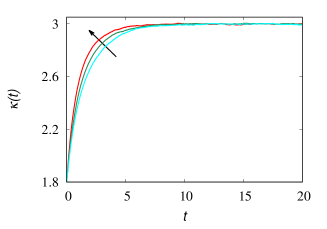
Figure 1: Kurtosis $\kappa(t)$ of the marginal ensemble distribution (for the first entry $z=z_{h,1}$ of ${\bf z}_{h}$) vs the normalized operational time $t=n/N$. The arrow indicates first the $d=2$ case (either with $\lambda=0$ or $\lambda=1/2$, that practically coincide), then the $d=3$ case at $\lambda=0$, and finally the $d=3$ case at $\lambda=1/2$.

To make an example, figure 1 depicts the evolution of the kurtosis $\kappa(t)$ vs the operational time $t=n/N$, (where $n$ is the number of CMT operations, and $N$ is the ensemble size) for the first ensemble entry $z_{h,1}$ at its convergence to the Gaussian limit $\kappa=3$ for $d=2,\,3$ and for two different values of $\lambda$ entering eq. (8). In this case $N=10^{6}$, and the entries of the initial ensamble are uniformly distributed with zero mean and unit variance. All the stochastic simulations refer to a random perturbation ${\bf r}$ uniformly distributed in $\partial S_{d}$. The equilibrium probability density for a larger ensemble $N=10^{9}$, starting from the same initial distribution is depicted in figure 1 at $d=3$, for $\lambda=0,\,1/2$ .

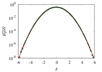
Figure 2: Equilibrium probability density functions for the third entry $z=z_{h,3}$ of ${\bf z}_{h}$, starting from the same initial conditions as in figure 1 for the CMT dynamics eq. (7). Symbols refer to stochastic simulations over an ensemble of $N=10^{9}$ elements: ($\circ$): $\lambda=0$, ($\square$): $\lambda=1/2$. The solid line represents the normal distribution.

The emergence of a limit Gaussian density in CMT is physics-dependent. Assuming the constraints eq. (3), this entirely depends on the form of the energy constaint eq. (4). In the presence of energy functions $e(|{\bf z}|)$ different from eq. (7) the stationary pdf for the entries of ${\bf z}$ is different from the Gaussian. This can be illustrated by means of a simple example of physical relevance. Consider the relativistic extension dunkel1 ; dunkel2 ; giona_rel , and consequently the energy function $e(|{\bf z}|)$ given by

$$e(|{\bf z}|)=\sqrt{|{\bf z}|\,c^{2}+m^{2}c^{4}}$$ (11)

corresponding to the relativistic energy of particle of mass $m$, provided that ${\bf z}$ represents its momentum, while keeping the linear constraints eq. (3). Set $m=1$, $c=1$ a.u.

CMT transformations can be applied on equal footing to this case, adopting for the transformations ${\bm{\phi}}$, ${\bm{\psi}}$ the functional form eq. (8). The case $\lambda=0$ is considered, where the group $\alpha_{\lambda}$ is defined in order to account for the structure of the energy function eq. (11). Figure 3 depicts the asymptotic (equilibrium) densities at $d=3$ for a generic entry of ${\bf z}_{h}$, at two different values of $E_{0}$. Data refer to an ensemble size of $N=10^{7}$, and the initial conditions are of impulsive nature. Each initial ${\bf z}_{h,k}^{(0)}$ attains with equal probability the values $\pm a$, where $a=\sqrt{(E_{0}^{2}-1)/3}$.

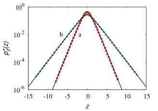
Figure 3: Equililibrium probability density functions $p_{z}^{*}(z)$ for the first entry $z=z_{h,1}$ of ${\bf z}$ for $d=3$ in the presence of the energy function eq. (11). Symbols are the results of stochastic simulations of the CMT with $E_{0}=2$ (symbols $\square$), and $E_{0}=3$ (symbols $\circ$). Lines (a) and (b) correspond to the Jüttner distribution eq. (12) at two values of the parameter $\beta$.

Deviation for the Gaussian behaviour is sensible, and the simulation data converge to the Jüttner distribution

$$p_{z}^{*}(z)=Ae^{-\beta\,\sqrt{z^{2}\,c^{2}+m^{2}\,c^{4}}}$$ (12)

where $A$ is the normalization constant, and the parameter $\beta$ is determined by the initial value $E_{0}$ of the ensemble average of $e(|{\bf z}|)$. The detailed analysis of the relativistic case is marginal in the present discussion, and it will thoroughly developed elsewhere. What is significant for the scope of this Letter is that Gaussianity in CMT’s is a consequence of the physical assumptions on the energy constraint.

To conclude, CMT’s provide the physical counterpart of CLT (which is strictly speaking a mathematical property), as regards the statistical characterization of kinetic variables (velocity, momentum), the dynamics of which is intrinsically distributional (owing to the conservation principles) and not additive. It can be stated, in a pictorial way, that while “kinematic Gaussianity” stems from CLT, as in the spatial propagation of Brownian motion, “dynamic Gaussianity”, as in equilibrium velocity and momentum distributions, is a consequence of CMT, with its imbedded supergeneric occurrence.

The definition of CMT finds another major application in the study of thermalization, and of equilibrium properties of molecular gases, in which, apart from particle-particle collisions, quantum effects, related to the structure of the quantized energy levels of the molecules, should be necessarility taken into account. This problem, that is an extension of the work by Einstein einstein1916 ; milonni on the momentum transfer by emission and absorption of radiation, and of the stochastic modeling of radiative effects PG_radiation will be developed in a forthcoming work.

References

- (1) M. Kac, Statistical Independence in Probability, Analysis & Number Theory, (Dover Publ., Mineola, 2018).
- (2) B. V. Gnedenko and A. N. Kolmogorov, Limit Distributions for Sums of Independent Random Variables, (Addison-Wesley, Reading, 1954).
- (3) V. V. Petrov, Sums of Independent Random Variables, (Springer-Verlag, New York, 1975).
- (4) P. Billingsley, Probability and Measure, (John Wiley & Sons, New York, 1995).
- (5) B. V. Gnedenko and V. Yu. Korolev, Random Summation (CRC Press, Boca Raton, 1996).
- (6) C. Stein, Proc. of the Sixth Berkeley Symp. on Math. Statist. and Probab., Vol. II: Probability theory, 1972, 583–602.
- (7) S. Chatterjee, arXiv:1404.1392, 2014.
- (8) M. Kardar, Statistical Physics of Particles (Cambridge Univ. Press, Cambridge, 2007).
- (9) M. Giona, A. Cairoli and R. Klages, J. Phys. A 55 (2022) 475002.
- (10) A. Einstein, Investigations on the Theory of Brownian Movement, (Dover Publ., Mineola, 1956).
- (11) S. Havlin and D. Ben-Avraham, Adv. Phys. 36 (1987) 695.
- (12) R. Klages, G. Radons and I. M. Sokolov (Eds.), Anomalous transport, (Wiley-VCH Verlag, Weinheim, 2008).
- (13) M. F. Shlesinger, B. J. West and J. Klafter J, Phys. Rev. Lett. 58, (1987) 1100.
- (14) V. Zaburdaev, S. Denisov and J. Klafter, Rev. Mod. Phys. 87, (2015) 483.
- (15) P. Lévy, Calcul dés Probabilités, (Gautier-Villars, Paris, 1925).
- (16) V. V. Uchaikin and V. M. Zolotarev, Chance and Stability: Stable Distributions and their Applications, (de Gruyter, Berlin, 1999).
- (17) W. Pauli, Theory of Relativity, (Dover Publ., Mineola, 1981).
- (18) S. Chapman and T. G. Cowling, The Mathematical Theory of Non-Uniform Gases, (Cambridge University Press, Cambridge, 1952).
- (19) S. Harris, An Introduction to the Theory of the Boltzmann Equation, (Dover Publ., Mineola, 2004).
- (20) P. Ehrenfest and T Ehrenfest, The Conceptual Foundations of the Statistical Approach in Mechanics, (Dover Publ., Mineola, 2014).
- (21) M. Mezard, G. Parisi and M. A. Virasoro, Sping Glass Theory and Beyond, (World Scientific, Singapore, 1987).
- (22) G. Jona-Lasinio, Il Nuovo Cimento 26 (1975) 99.
- (23) P. Goswami and S. Chakravarty, Phys. Rev. B 95 (2017) 075131.
- (24) J. Dunkel and P. Hänggi, Phys. Rep. 471 (2009) 1.
- (25) J. Dunkel, P. Talkner and P. Hänggi, New J. Phys. 9 (2007) 144.
- (26) M. Giona, EPL 126 (2019) 50001.
- (27) A. Einstein, Phys. Zeit. 18 (1917) 121.
- (28) P. W. Milonni, The Quantum Vacuum. An introduction to Quantum Electrodynamics, (Academic Press, San Diego, 1994).
- (29) C. Pezzotti and M. Giona, Particle-photon radiative interactions and thermalization, (2022) in preparation.