An Analytical Theory for the Growth from Planetesimals to Planets by Polydisperse Pebble Accretion

Abstract

Pebble accretion is recognized as a significant accelerator of planet formation. Yet, only formulae for single-sized (monodisperse) distribution have been derived in the literature. These can lead to significant underestimates for Bondi accretion, for which the best accreted pebble size may not be the one that dominates the mass distribution. We derive in this paper the polydisperse theory of pebble accretion. We consider a power-law distribution in pebble radius, and we find the resulting surface and volume number density distribution functions. We derive also the exact monodisperse analytical pebble accretion rate for which 3D and 2D accretion are limits. In addition, we find analytical solutions to the polydisperse 2D Hill and 3D Bondi limits. We integrate the polydisperse pebble accretion numerically for the MRN distribution, finding a slight decrease (by an exact factor 3/7) in the Hill regime compared to the monodisperse case. In contrast, in the Bondi regime, we find 1-2 orders of magnitude higher accretion rates compared to monodisperse, also extending the onset of pebble accretion to 1-2 order of magnitude lower in mass. We find Myr-timescales, within the disk lifetime, for Bondi accretion on top of planetary seeds of masses $10^{-6}-10^{-4}M_{\oplus}$, over a significant range of the parameter space. This mass range overlaps with the high mass end of the planetesimal initial mass function, and thus pebble accretion is possible directly following formation by streaming instability. This alleviates the need for mutual planetesimal collisions as a major contribution to planetary growth.

1 Introduction

Despite significant theoretical and observational advances in the past decade, a comprehensive theory of planet formation still remains elusive. Planet formation starts from the accumulation of sub-$\mu$m interstellar grains, growing by means of coagulation, in hit-and-stick low-velocity collisions (Safronov, 1972; Nakagawa et al., 1981; Tominaga et al., 2021). Laboratory experiments (Blum & Wurm, 2008; Güttler et al., 2010) and numerical simulations (Güttler et al., 2009; Geretshauser et al., 2010; Zsom et al., 2010) provide evidence that this process is efficient in growing solid grains up to mm and cm radius (hereafter called “pebbles”) with growth beyond this size being unlikely, due to bouncing, fragmentation, and drift (Dullemond & Dominik, 2005; Brauer et al., 2008; Krijt et al., 2015), unless the possibility of very high porosities is introduced (Suyama et al., 2008, 2012).

The streaming instability (Youdin & Goodman, 2005; Youdin & Johansen, 2007; Johansen & Youdin, 2007; Kowalik et al., 2013; Lyra & Kuchner, 2013; Krapp et al., 2019; Squire & Hopkins, 2020; Schäfer et al., 2020; Paardekooper et al., 2020; Chen & Lin, 2020; McNally et al., 2021; Lin, 2021; Flock & Mignone, 2021; Zhu & Yang, 2021; Yang & Zhu, 2021) whereby the drift of grains through the gas is unstable, has been established as a mechanism to produce the first planetesimals (Johansen et al., 2007; Yang & Johansen, 2014; Carrera et al., 2015; Simon et al., 2016; Yang et al., 2017; Schaffer et al., 2018; Nesvorný et al., 2019; Li et al., 2019; Klahr & Schreiber, 2021; Visser et al., 2021; Li & Youdin, 2021), through concentration of pebbles into dense filaments that display a fractal structure with large overdensities reached at the smallest scales of the simulations (Johansen et al., 2015). Yet, growth by binary accretion of planetesimals into progressively larger objects, while able to explain the growth of a giant planet’s core at 5 AU (if migration is ignored, Pollack et al., 1994), is not viable already at the orbital position of Saturn, Uranus, or Neptune (Thommes et al., 2003; Johansen & Bitsch, 2019).

This shortcoming of planetesimal accretion motivated the search for other avenues of planetary growth. Fast accretion rates of marginally coupled solids up to planetary masses were first seen in the simulations of Lyra et al. (2008). In that model, vortices trap pebbles and collapse them into Moon-mass objects via direct gravitational instability, which scoop up the remaining pebbles at a vertiginous rate, achieving Mars and Earth mass within a few hundred orbits. Whereas this growth was assisted by vortices, it illustrates that gas-assisted accretion of pebbles is potentially much faster than planetesimal accretion, due to the presence of gas drag as a dissipative mechanism. A similar result was found by Johansen & Lacerda (2010), showing fast accretion rates onto a 100 km seed, highlighting the importance of pebble accretion for planetary growth, and suggesting for the first time that a significant fraction of the accretion of planetary bodies proceeds via pebbles (as opposed to planetesimals), before the dissipation of the gas disk.

An analytical theory of pebble accretion was later developed by Ormel & Klahr (2010) and Lambrechts & Johansen (2012), elucidating the existence of two regimes: one for small masses, where the seed mass accretes from a pebble headwind, a process reminiscent of Bondi-Hoyle-Lyttleton accretion (Bondi & Hoyle, 1944; Hoyle & Lyttleton, 1939); and another, for higher masses, where pebbles are accreted from the whole Hill sphere of the seed. These regimes were dubbed “drift-dominated” and “shear-dominated” by Ormel & Klahr (2010), respectively, whereas Lambrechts & Johansen (2012) called them “Bondi” and “Hill”. As a rule of thumb, planetesimals accrete in the Bondi regime, protoplanets in the Hill regime (Ormel, 2017; Johansen & Lambrechts, 2017), and both can yield orders-of-magnitude higher mass accretion rates than planetesimal accretion.

Since its inception, the model has quickly risen to paradigmatic status, by virtue of a number of successes. Pebble accretion explains the formation of the gas giants (Lambrechts & Johansen, 2012), of the ice giants with low gas fractions (Lambrechts et al., 2014); the preponderance of super-Earths around other stars (Lambrechts et al., 2019; Bitsch et al., 2019b; Izidoro et al., 2021); it achieves a better planet population synthesis matching exoplanet populations than a planetesimal-based accretion model (Bitsch et al., 2019a; Drazkowska et al., 2022), and it is also compatible with the drift-dominated evolution of dust in T-Tauri disks (a flux of $\sim$ 100 Earth masses over the disk lifetime, Appelgren et al. 2020). Even the classical giant impact model for terrestrial planet formation (Raymond et al., 2004) is challenged now by a hybrid view where terrestrial planets accrete their mass from a combination of planetesimals and small pebbles (Johansen et al., 2015, 2021).

However, most previous works on pebble accretion considered a monodisperse distribution of pebbles. In reality, the pebbles will have a distribution of sizes, ranging from sub-$\mu$m to mm or cm-size. A monodisperse distribution can be a reasonable assumption because, for the interstellar grain size distribution, following a power-law of -3.5 of the grain radius (Mathis et al., 1977; Hirashita & Kobayashi, 2013, MRN henceforth) most of the mass resides in the largest pebbles; a result that stands even after dust evolution away from MRN in the protoplanetary disk is considered (Birnstiel et al., 2012). This makes the Hill regime of pebble accretion relatively insensitive to the dust spectrum, and either the dominant pebble size (Lambrechts & Johansen, 2014) or a mass weighted representative pebble size (Guilera et al., 2020; Venturini et al., 2020) yield sensible results.

Indeed, in a recent work, Andama et al. (2022), considering polydisperse Hill accretion, find larger final core masses, not because of faster accretion rates, but because the smaller grains drift more slowly, lingering around for longer times than the largest pebbles, and thus extending the duration of accretion. Drażkowska et al. (2021) also considering the Hill regime, focus on the beneficial aspects of fragmentation on keeping the pebbles sizes small, because too large pebbles accrete poorly. Both works consider a body already near the Bondi-Hill transition mass, a polydisperse size spectrum from the prescription of Birnstiel et al. (2012), and solve numerically for the mass accretion rates. Both works also highlight how the mass accretion rate is dependent on the embryo mass but not on pebble size.

In stark constrast, in the Bondi regime the size distribution should matter significantly for the mass accretion rate itself. In the Bondi regime, the best accreted pebbles are those of friction time similar to the time the pebble takes to cross the Bondi radius, i.e., the Bondi time. For small enough seed mass, the larger, cm-sized, pebbles, drift so fast past the protoplanet that these pebbles essentially behave like planetesimals. In this case, the cross section for accretion is geometric (for high speeds), or gravitationally focused (for low speeds), and only slightly aided by gas drag. As a result, even though these pebbles dominate the mass budget, their mass accretion rate by the planetesimal can be lower than of the smaller pebbles for which Bondi accretion is more efficient. If that is the case, the pebble accretion rates in the Bondi regime may be underestimated by the current monodisperse prescriptions. Indeed, Lorek & Johansen (2022) recently find that planetesimal accretion is insignificant beyond 5 AU, so the onset of pebble accretion has to overlap with the high-mass end of the planetesimal mass function if planet formation is to proceed.

In this paper, we work out the polydisperse extension of pebble accretion. We find that indeed Bondi accretion is 1-2 orders of magnitude more efficient in the polydisperse case. We also find that the onset of polydisperse Bondi accretion occurs at lower masses than monodisperse, by 1-2 orders of magnitude. Hill accretion is slightly less efficient, by a factor 3/7, for the MRN distribution. We find the exact solution to the 2D-3D transition, as well as analytical expressions for the polydisperse 2D Hill and 3D Bondi accretion rates.

This paper is structured as follows. In Sect. 2 we derive the grain size distribution functions; in Sect. 3 we apply them to pebble accretion, deriving the polydisperse model, and proceeding with the analysis. In Sect. 4 we work out the analytical expressions for 2D Hill and 3D Bondi polydisperse accretion. A summary concludes the paper in Sect. 7. A table of mathematical symbols used in this work is shown in

table:symbols.

Table 1: Symbols used in this work.

Symbol	Definition	Description		Symbol	Definition	Description
$F$	Eq. (1)	pebble size distribution		$\rho_{d0}$	Eq. (39)	dust density at midplane
$a$		pebble radius		$\delta v$	Eq. (40)	approach velocity
$z$		vertical coordinate		$S$	Eq. (34)	stratification integral
$n$	Eq. (2)	number density		$\Delta v$		Sub-Keplerian velocity reduction
$m$	Eq. (7)	pebble mass		$\varOmega$	$\sqrt{\frac{GM_{\odot}}{r^{3}}}$	Keplerian frequency
$\rho_{d}$	Eq. (3)	volume density		$\hat{R}_{\rm acc}$	Eq. (53)	accretion radius
$H_{d}$	Eq. (5)	pebble scale height		$\chi$	Eq. (41)	coefficient
$f$	Eq. (22)	pebble distribution in midplane		$\tau_{f}$	$\mathrm{St}/\varOmega$	friction time
$H_{g}$	$\varOmega/c_{s}$	gas scale height		$t_{p}$	Eq. (42)	passing timescale
$\alpha$		Shakura-Sunyaev viscosity		$\gamma$	Eq. (41)	coefficient
$\mathrm{St}$	Eq. (6)	Stoker number		$G$		gravitational constant
$\rho_{\bullet}$		internal pebble density		$M_{p}$		planetesimal mass
$\varSigma_{g}$	Eq. (23)	gas column density		$R_{H}$	Eq. (43)	Hill radius
$\varSigma_{d}$	$Z\varSigma_{g}$	pebble column density		$t_{B}$	Eq. (47)	Bondi time
$k$	Eq. (14)	power law of unsedimented distribution		$R_{B}$	Eq. (46)	Bondi radius
$p$	Eq. (16)	power law of column density distribution		$M_{t}$	Eq. (49)	transition mass
$q$	Eq. (17)	power law of internal density		$M_{\rm HB}$	Eq. (48)	Hill-Bondi transition mass
$D$	Eq. (20)	Coefficient of column density distribution		$R$	$\sqrt[3]{\frac{3M_{p}}{4\pi\rho_{\bullet}}}$	planetesimal radius
$Z$	$\varSigma_{d}/\varSigma_{g}$	Dust-to-gas ratio		$v_{\rm esc}$	$\sqrt{\frac{2GM_{p}}{R}}$	escape velocity
$\rho_{\bullet}^{(0)}$		internal density of largest grain		$\mathrm{St}_{p}$	Eq. (51)	Stokes number past planetesimal
$r$		radial coordinate		$M_{\rm BL}$	Eq. (52)	Bondi-geometric transition mass
$r_{c}$	Eq. (23)	cutoff radius		$t_{\rm acc}$	Eq. (54)	accretion time
$W$	Eq. (27)	column density distribution		$h$	$H_{g}/r$	aspect ratio
$R_{\rm acc}$	Eq. (41)	drag-modified accretion radius		$m_{p}$		characteristic streaming instability mass
$\xi$	Eq. (41)	coefficient		$\psi$	Eq. (64)	shorthand
$\dot{M}$		mass accretion rate		$T$	Eq. (24)	gas temperature
$c_{s}$	$\sqrt{Tc_{p}(\Gamma-1)}$	sound speed		$\Gamma$		adiabatic index
$\mu$		mean molecular weight		$c_{p}$	$\frac{R_{\rm gas}}{\mu}\frac{\Gamma}{\left(\Gamma-1\right)}$	specific heat at constant pressure
$R_{\rm gas}$		gas constant		$c_{v}$	$c_{p}/\Gamma$	specific heat at constant volume

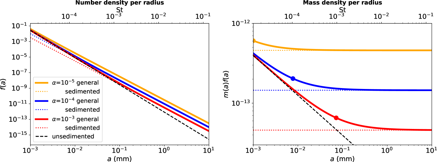
Figure 1: Left: The grain distribution function $f(a)$ in the midplane. Integrated over $a$, this function yields the number density $n$ in the midplane. This model is calculated at 20 AU with density and temperature according to Eqs. (23) and (24), $Z=0.01$, constant $\rho_{\bullet}$, and MRN (unsedimented, $\mathrm{St}\ll\alpha$, black dashed line). Three values of $\alpha$ are shown (solid lines). The “sedimented” limits ($\mathrm{St}\gg\alpha$, dotted lines) are shown for comparison. Right: mass density distribution, i.e., the left panel multiplied by the mass of a pebble. Integrated, this function yields the grain density $\rho_{d0}$ in the midplane. The distributions follow the unsedimented line for $\mathrm{St}\lesssim\alpha$, and the sedimented line for $\mathrm{St}\gtrsim\alpha$, as expected. The mass function is constant with $a$ in the sedimented limit because of the MRN choice: the $a^{-3.5}$ power law is canceled by the combination of the mass of the particle $a^{3}$ and the extra $\sqrt{a}$ dependency from the sedimentation. Large dots mark the point where $\mathrm{St}=\alpha$.

2 Distribution Functions

Consider the grain size distribution

$$F(a,z)\equiv\frac{\partial n}{\partial a}$$ (1)

that defines the number density $n$; here, $a$ is the grain radius and $z$ the vertical coordinate. We integrate it to yield

$$n(a,z)=\int_{0}^{a}F(a^{\prime},z)\ da^{\prime},$$ (2)

and $n(z)\equiv n(a_{\rm max},z)$. The volume density is found by multiplying $F(a,z)$ by the mass $m(a)$ of a single grain

$$\rho_{d}(a,z)=\int_{0}^{a}m(a^{\prime})\ F(a^{\prime},z)\ da^{\prime}.$$ (3)

and again, $\rho_{d}(z)\equiv\rho_{d}(a_{\rm max},z)$. Due to sedimentation, we can write, for an equilibrium between diffusion and gravity (Dubrulle et al., 1995)

$$F(a,z)\equiv f(a)\ e^{-z^{2}/2H_{d}^{2}},$$ (4)

defining the function $f(a)$, which is the size distribution function in the midplane. In Eq. (4), $H_{d}$ is the grain scale height, a function of $a$ (Klahr & Henning, 1997; Lyra & Lin, 2013)

$$H_{d}=H_{g}\ \sqrt{\frac{\alpha}{\mathrm{St}+\alpha}},$$ (5)

where $H_{g}$ is the gas scale height, $\alpha$ is a dimensionless vertical diffusion parameter, and $\mathrm{St}$ is the Stokes number, a non-dimensionalization of the grain radius, normalized by the grain internal density $\rho_{\bullet}$ and the gas column density $\varSigma_{g}$

$$\mathrm{St}\equiv\frac{\pi}{2}\frac{a\ \rho_{\bullet}}{\varSigma_{g}}.$$ (6)

2.1 The distribution function in the midplane

To find $f(a)$, consider spherical grains

$$m(a)=\frac{4\pi}{3}a^{3}\rho_{\bullet}$$ (7)

and the column density

$$\varSigma_{d}(a)\equiv\int_{-\infty}^{\infty}\rho_{d}(a,z)\ dz.$$ (8)

Substituting Eq. (3), and integrating in $z$, we find

$$\varSigma_{d}(a)=\frac{2^{5/2}\pi^{3/2}}{3}\int_{0}^{a}\rho_{\bullet}\ H_{d}\ a^{\prime}\,{}^{3}\ f(a^{\prime})\ da^{\prime},$$ (9)

and the total column density $\varSigma_{d}\equiv\varSigma_{d}(a_{\rm max})$. We keep the internal density $\rho_{\bullet}$ inside the integral because it is in general a function of radius, if grains have different composition. Given

$$\varSigma_{d}(a)=\int_{0}^{a}\frac{\partial\varSigma_{d}(a^{\prime})}{\partial a^{\prime}}da^{\prime},$$ (10)

we find, equating the integrands of Eq. (9) and Eq. (10), and solving for $f(a)$

$$f(a)=\frac{3}{2^{5/2}\pi^{3/2}H_{g}\rho_{\bullet}}\sqrt{1+\frac{\mathrm{St}}{\alpha}}\ a^{-3}\frac{\partial\varSigma_{d}(a)}{\partial a},$$ (11)

where we also substituted Eq. (5) for $H_{d}$ as a function of $\mathrm{St}$. The distribution is determined if we find an expression for $\partial_{a}\varSigma_{d}(a)$.

2.1.1 Sedimented and unsedimented limits

To find the general solution, we need to find the expression for $\partial_{a}\varSigma_{d}$ in Eq. (11). We do so by realizing that even though the midplane volume density is modified by sedimentation, the column density $\varSigma_{d}$ is not. The two limits of $f(a)$ are, first, the “sedimented” limit, for $\mathrm{St}\gg\alpha$

$$f(a)^{({\rm sed})}=\frac{3}{8\pi H_{g}\rho_{\bullet}^{1/2}\varSigma_{g}^{1/2}\alpha^{1/2}}\ a^{-2.5}\frac{\partial\varSigma_{d}(a)}{\partial a},$$ (12)

and, second, the unsedimented limit, for $\mathrm{St}\ll\alpha$

$$f(a)^{({\rm unsed})}=\frac{3}{2^{5/2}\pi^{3/2}H_{g}\rho_{\bullet}}\ a^{-3}\frac{\partial\varSigma_{d}(a)}{\partial a},$$ (13)

where we have substituted the Stokes number given by Eq. (6). Since the column density does not change with sedimentation, we can find $\partial_{a}\varSigma_{d}$ by either limit.

We assume a power-law dependency for the unsedimented distribution in the midplane

$$f(a)^{({\rm unsed})}\ \propto\ a^{-k}$$ (14)

where $k$ is a constant (the MRN distribution corresponds to $k=3.5$). Equating Eq. (13) and Eq. (14)

$$\frac{\partial\varSigma_{d}(a)}{\partial a}\propto\rho_{\bullet}\ a^{3}\ a^{-k}.$$ (15)

We thus write

$$\frac{\partial\varSigma_{d}(a)}{\partial a} \propto a^{-p};$$ (16)

$$\rho_{\bullet} \propto a^{-q};$$ (17)

$$p-q = k-3.$$ (18)

We can then write the column density distribution as a power law

$$\frac{\partial\varSigma_{d}(a)}{\partial a}=D\ a^{-p}.$$ (19)

Integrating it in $a$, equating to Eq. (10), and solving for the constant $D$, we find

$$D=\frac{(1-p)Z\varSigma_{g}}{a_{\rm max}^{1-p}};$$ (20)

here we also substitute $\varSigma_{d}=Z\varSigma_{g}$, where $Z$ is the metallicity. Considering now the variation of the internal density

$$\rho_{\bullet}(a)=\rho_{\bullet}^{(0)}\left(\frac{a}{a_{\rm max}}\right)^{-q},$$ (21)

the full distribution is found at last

$$f(a)=\frac{3(1-p)Z\varSigma_{g}}{2^{5/2}\pi^{3/2}H_{g}\rho_{\bullet}^{(0)}a_{\rm max}^{4-k}}\sqrt{1+a\frac{\pi}{2}\frac{\rho_{\bullet}(a)}{\varSigma_{g}\alpha}}\ a^{-k}.$$ (22)

Notice that to keep $f(a)$ positive definite, the solution requires $p<1$. For $q=0$, Eq. (18) constrains $k<4$.

The gas density used is

$$\varSigma_{g}=10^{3}\,{\rm g\,cm}^{-2}\ \left(\frac{r}{\rm AU}\right)^{-1}\ e^{-r/r_{c}}$$ (23)

i.e. the self-similar solution to the viscous evolution equations (Lynden-Bell & Pringle, 1974). Here $r$ is the distance to the star, and $r_{c}$ a truncation radius. We choose $r_{c}=$100 AU. For the temperature, we use the irradiated, radially optically thick, vertically optically thin model of Kusaka et al. (1970, see also )

$$T=150\,{\rm K}\ \left(\frac{r}{\rm AU}\right)^{-3/7}$$ (24)

In addition, we assume metallicity $Z=0.01$, adiabatic index 1.4, and mean molecular weight 2.3.

We plot the resulting distributions in Fig. 1, for 20 AU, maximum grain size $a_{\rm max}=1$ cm, and $k=-3.5$. For internal density we use $\rho_{\bullet}^{(0)}=3.5$ g cm^-3 and $q=0$. The left panel shows $f(a)$; the right panel $m(a)f(a)$. The functions are shown for three values of $\alpha$ (solid lines). The unsedimented ($\mathrm{St}\ll\alpha$, black dashed line) and “sedimented” ($\mathrm{St}\gg\alpha$, dotted lines) limits are shown for comparison. We see that the sedimented distributions follow the unsedimented line for $\mathrm{St}\lesssim\alpha$, and the sedimented line for $\mathrm{St}\gtrsim\alpha$, as expected. The flat profile for the sedimented cases is due to the MRN exponent, coupled with $\sqrt{\mathrm{St}}$ from the sedimentation.

2.2 Column density

For completeness, we define the vertically-integrated grain size distribution

$$W(a)\equiv\int_{-\infty}^{\infty}F(a,z)\ dz=\sqrt{2\pi}\ H_{d}\ f(a),$$ (25)

so that the pebble column density is

$$\varSigma_{d}(a)=\int_{0}^{a}m(a^{\prime})\ W(a^{\prime})\ da^{\prime}.$$ (26)

Substituting Eq. (22) in Eq. (25), we find the column density distribution function

$$W(a)=\frac{3(1-p)Z\varSigma_{g}}{4\pi\rho_{\bullet}^{(0)}a_{\rm max}^{4-k}}\ a^{-k},$$ (27)

which indeed yields $\varSigma_{d}=Z\varSigma_{g}$ when integrated according to Eq. (26).

3 Pebble Accretion

Having found the size distribution function for the pebble density, we are in position to apply it to pebble accretion. Pebble accretion is usually split into three regimes of accretion (loosely coupled, Bondi, and Hill accretion), each with 2D and 3D limits. We start by deriving the exact solution for the 2D-3D transition.

3.1 Exact solution for the monodisperse 2D-3D transition

The 3D and 2D limits of pebble accretion correspond to whether or not the accretion is embedded, i.e, if the accretion radius $R_{\rm acc}$ exceeds the height of the pebble column. The quantity governing the transition is $R_{\rm acc}/H_{d}$, or rather

$$\xi\equiv\left(\frac{R_{\rm acc}}{2H_{d}}\right)^{2},$$ (28)

which we will show a posteriori. The monodisperse mass accretion rates in these limits are (Lambrechts & Johansen, 2012)

$$\dot{M}_{\rm 3D} = \lim_{\xi\rightarrow 0}\dot{M}=\pi R_{\rm acc}^{2}\rho_{d0}\delta v,$$ (29)

$$\dot{M}_{\rm 2D} = \lim_{\xi\rightarrow\infty}\dot{M}=2R_{\rm acc}\varSigma_{d}\delta v,$$ (30)

where $\delta v$ is the velocity at which the pebble approaches the accretor, and $\rho_{d0}$ is the midplane density. In principle, we could apply Eq. (3) with Eq. (22) on Eq. (29); and Eq. (26) with Eq. (27) on Eq. (30), working with the two limits separately. Yet, given that $\xi$ is a function of grain size, and there are other transitions to deal with (loose coupling/Bondi/Hill), it is preferable to work with a general expression for $\dot{M}$, which we derive in this section.

Considering parallel horizontal chords of infinitesimal thickness in the vertical direction until the full accretion radius is taken into account, the general expression for the mass accretion rate is

$$\dot{M}=\int_{-R_{\rm acc}}^{R_{\rm acc}}2\sqrt{R_{\rm acc}^{2}-z^{2}}\ \rho_{d0}\ {\rm exp}\left(-\frac{z^{2}}{2H_{d}^{2}}\right)\delta v\ dz.$$ (31)

Following Johansen et al. (2015) we define the stratification integral

$$S\equiv\frac{1}{\pi R_{\rm acc}^{2}}\int_{-R_{\rm acc}}^{R_{\rm acc}}2\sqrt{R_{\rm acc}^{2}-z^{2}}\ {\rm exp}\left(-\frac{z^{2}}{2H_{d}^{2}}\right)\ dz,$$ (32)

so that the mass accretion rate is generalized into one expression as

$$\dot{M}=\pi R_{\rm acc}^{2}\rho_{d0}\ S\ \delta v.$$ (33)

While Johansen et al. (2015) use a square approximation for the accretion radius, we find the exact solution of the stratification integral

$$S=e^{-\xi}\left[I_{0}(\xi)+I_{1}(\xi)\right],$$ (34)

where $I_{\nu}(\xi)$ are the modified Bessel functions of the first kind, and $\xi$ is given by Eq. (28). The exact monodisperse accretion rate is

$$\dot{M}=\pi R_{\rm acc}^{2}\rho_{d0}\,\delta v\,e^{-\xi}\left[I_{0}(\xi)+I_{1}(\xi)\right].$$ (35)

Indeed for $\xi\rightarrow 0$, the Bessel functions tend to $I_{0}(0)=1$, $I_{1}(0)=0$, and we recover 3D accretion (Eq. 29). For $\xi\rightarrow\infty$, both Bessel functions tend to $e^{\xi}/\sqrt{2\pi\xi}$, and 2D accretion is recovered (Eq. 30). Fig. 2 shows the agreement graphically. The square approximation is shown for comparison.

3.2 Polydisperse prescription

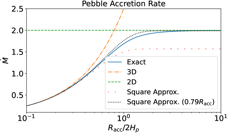
Figure 2: General expression for the monodisperse pebble accretion rate (Eq. 35). The 3D and 2D limits (eqs 29 and 30, respectively) are recovered. The square approximation is also shown for comparison.

To generalize Eq. (35) into a polydisperse description, we consider the integrated polydisperse accretion rate to be $\dot{M}\equiv\dot{M}(a_{\rm max})$, where

$$\dot{M}(a)=\int_{0}^{a}\frac{\partial\dot{M}(a^{\prime})}{\partial a^{\prime}}da^{\prime},$$ (36)

with

$$\frac{\partial\dot{M}(a)}{\partial a}=\pi R_{\rm acc}^{2}(a)\ \delta v(a)\ S(a)\ m(a)\ f(a).$$ (37)

Indeed, Eq. (36) with the integrand given by Eq. (37) is equivalent to Eq. (35) if

$$\int_{0}^{a_{\rm max}}R_{\rm acc}^{2}(a)\ \delta v(a)\ S(a)\ m(a)\ f(a)da=\bar{R}_{\rm acc}^{2}\ \overline{\delta v}\ \bar{S}\,\rho_{d0},$$ (38)

where the overline denotes that the quantity is an “effective” quantity, independent of pebble size. If the accretion radius $R_{\rm acc}$, the approach velocity $\delta v$, and the stratification integral $S$ were independent of the grain radius $a$, Eq. (38) would be exactly equivalent to replacing the midplane dust density by the integrated grain size distribution

$$\rho_{d0}=\int_{0}^{a_{\rm max}}m(a)f(a)da,$$ (39)

which is intuitive. We can now use much of the formalism of pebble accretion already derived in the literature. The approach velocity $\delta v$ is given by

$$\delta v\equiv\Delta v+\varOmega R_{\rm acc},$$ (40)

where $\Delta v$ is the sub-Keplerian velocity reduction and $\varOmega$ is the Keplerian frequency. The accretion radius is (Ormel & Klahr, 2010)

$$R_{\rm acc}\equiv\hat{R}_{\rm acc}{\rm exp}\left[-\chi(\tau_{f}/t_{p})^{\gamma}\right],$$ (41)

where $\tau_{f}=\mathrm{St}/\varOmega$ is the pebble friction time, $\chi=0.4$ and $\gamma=0.65$ are empirically-determined coefficients, and

$$t_{p}\equiv\frac{GM_{p}}{\left(\Delta v+\varOmega R_{H}\right)^{3}}$$ (42)

is the characteristic passing time scale. Here $G$ is the gravitational constant, $M_{p}$ the mass of the planetesimal, and $R_{H}$ its Hill radius

$$R_{H}\equiv\left(\frac{GM_{p}}{3\varOmega^{2}}\right)^{1/3}.$$ (43)

The variable $\hat{R}_{\rm acc}$ depends on the accretion regime. For Hill accretion it is

$$\hat{R}_{\rm acc}^{\rm(Hill)}=\left(\frac{\mathrm{St}}{0.1}\right)^{1/3}R_{H},$$ (44)

and for Bondi accretion it is

$$\hat{R}_{\rm acc}^{\rm(Bondi)}=\left(\frac{4\tau_{f}}{t_{B}}\right)^{1/2}R_{B},$$ (45)

where

$$R_{B}\equiv\frac{GM_{p}}{\Delta v^{2}}$$ (46)

is the Bondi radius and

$$t_{B}\equiv\frac{R_{B}}{\Delta v}$$ (47)

is the Bondi time. The transition mass between Bondi and Hill accretion is defined by (Ormel, 2017)

$$M_{HB}=\frac{M_{t}}{8\mathrm{St}},$$ (48)

where

$$M_{t}\equiv\frac{\Delta v^{3}}{G\varOmega}.$$ (49)

A third regime also exists, of accretion of loosely coupled pebbles, for which the accretion radius is the physical radius $R$ augmented by the gravitational focusing cross-section

$$R_{\rm acc}^{\rm(geo)}=R\sqrt{1+\frac{v_{\rm esc}^{2}}{\Delta v^{2}}},$$ (50)

where $v_{\rm esc}$ is the escape velocity of the planetary seed. In this regime the grains are so loosely coupled they behave almost like planetesimals, except for small enough grains, that remain coupled to the gas and follow the gas streamlines. The quantity that defines this latter transition is (Ormel, 2017)

$$\mathrm{St_{p}}=\frac{\Delta v\ \tau_{f}}{R},$$ (51)

that is, the friction time normalized by the time to pass past the planetesimal; a planetesimal Stokes number (hence the “p” in $\mathrm{St_{p}}$). For $\mathrm{St_{p}}<1$, we set $R_{\rm acc}^{\rm(geo)}=0$. The transition mass $M_{BL}$ between Bondi and loosely coupled accretion happens at (Ormel, 2017)

$$M_{BL}=\frac{M_{t}}{8}\mathrm{St}.$$ (52)

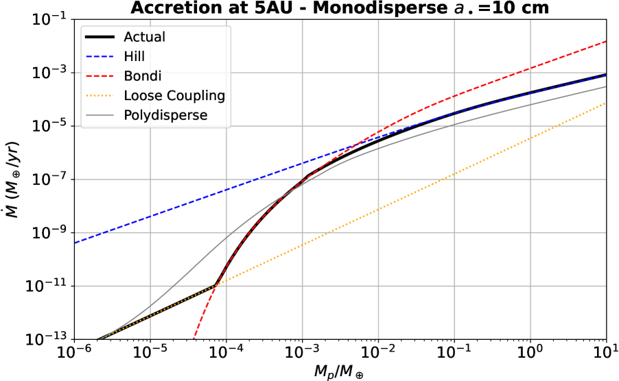
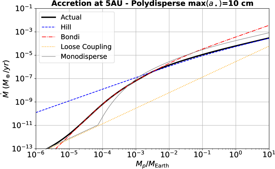
Figure 3: Comparison between monodisperse (left) and the integrated polydisperse (right) accretion rates (Eq. 36). The left panel uses the parameters of Fig. 4 of Johansen & Lambrechts (2017), except that we use the monodisperse general equation here derived (Eq. 35). A pebble size of 10 cm is not supported by observations but we keep this size for benchmarking purposes. The polydisperse accretion rate is reproduced in the left plot, and the monodisperse accretion rate in the right plot (grey lines), for comparison. The Hill accretion yields a lower accretion rate (3/7 lower than monodisperse) because other pebbles sizes are present, not only $a=10$ cm. The main difference is the accretion rate for polydisperse Bondi accretion being up to two orders of magnitude more efficient than monodisperse, and the onset of pebble accretion happening over one order of magnitude lower in mass. This occurs because the best-accreted pebble is not present in the monodisperse distribution, and $a_{\rm max}$ is too loosely coupled, accreting poorly. Notice the smooth transition from Bondi to Hill accretion with the exact 2D-3D transition.

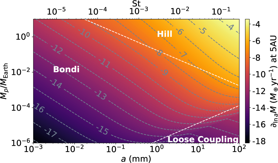
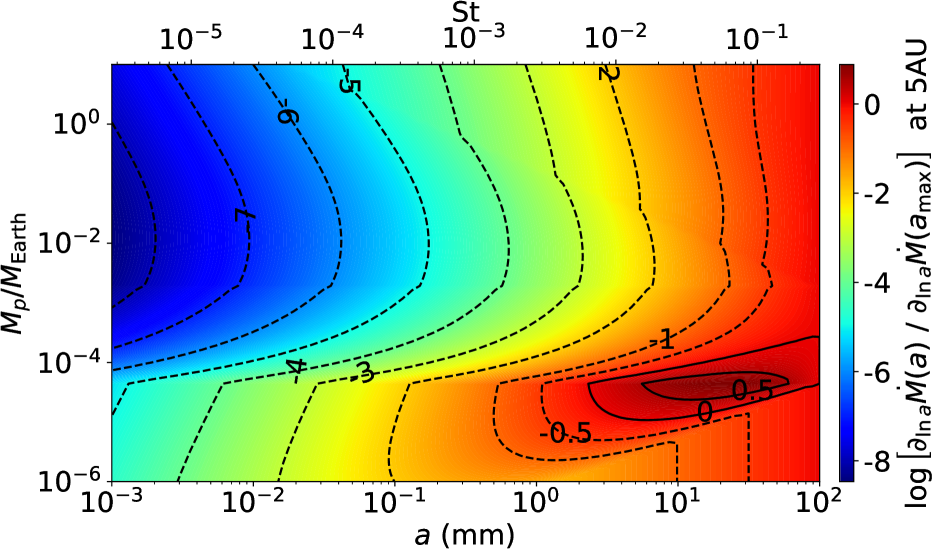
Figure 4: Left: The polydisperse pebble accretion rate $\partial_{\,\ln\,a}\,\dot{M}$ (Eq. 37), as a function of grain radius. In the Hill accretion regime the largest pebble present dominates the mass accretion rate. Conversely, for Bondi accretion, we see that at a given seed mass the differential accretion rate is non-monotonic with grain size. For low enough seed masses, the biggest grains, although dominating the mass distribution, accrete in the loosely coupled regime. Right: Same as the left plot, but normalized by the accretion rate for $a_{\rm max}$ (proxy for monodispersive). The bright red contours are the regions were polydisperse accretion is enhanced over monodisperse. We see that it mostly corresponds to the region where monodisperse is in the loosely coupled regime, but polydisperse is already in Bondi. The best accreted pebbles are those for which the stopping time $\tau_{f}$ equals the Bondi time $t_{B}$. Absent in the monodispersive description, these pebbles may contribute less to the mass budget, but their enhanced accretion ends up dominating the mass accretion rate.

3.3 Polydisperse vs Monodisperse

We show in the left panel of Fig. 3 a reproduction of the monodisperse accretion rates from Johansen & Lambrechts (2017), for $a=$ 10 cm, and at 5 AU. Even though the observations do not support the existence of these large grains, we use it for benchmark purposes. The different lines show the pebble accretion rates in the Hill and Bondi regimes, as well as the loosely coupled regime for low masses.

The Hill limit (blue dashed line) is recovered for Eq. (35) with $\hat{R}_{\rm acc}$ given by Eq. (44), and $\delta v=\varOmega R^{(\rm Hill)}_{\rm acc}$. The Bondi limit (red dashed line) is recovered for Eq. (35) with $\hat{R}_{\rm acc}$ given by Eq. (45), and $\delta v=\Delta v+\varOmega R^{(\rm Bondi)}_{\rm acc}$. The actual solution (black thick line) uses

$$\hat{R}_{\rm acc}=\left\{\begin{array}[]{ll}\hat{R}_{\rm acc}^{(\rm Hill)}&{\rm if}\ M\geq M_{\rm HB},\\ \hat{R}_{\rm acc}^{(\rm Bondi)}&{\rm if}\ M<M_{\rm HB},\end{array}\right.$$ (53)

and the general $\delta v$ given by Eq. (40). The mass accretion rate is then the maximum between this and the loosely coupled accretion rates. The loosely coupled regime is given by Eq. (35) with $\delta v=\Delta v$ and $R_{\rm acc}$ given by Eq. (50) if $\mathrm{St_{p}}\geq 1$, and zero otherwise.

The right panel of Fig. 3 shows how the accretion rates differ when we include a particle size distribution. In this panel we are showing the integrated accretion rate $\dot{M}\equiv\dot{M}(a_{\rm max})$ given by Eq. (36). The monodisperse line is shown for comparison.

3.3.1 Slightly lower efficiency in the Hill regime

From comparing the plots in Fig. 3, we see that the polydisperse accretion rate is slightly lower in the regime of Hill accretion; this occurs because, in the Hill regime, there is less mass at the biggest pebble size $a_{\rm max}$ compared to monodisperse (where all pebbles are of 10 cm). We work out in Sect. 4 this reduction factor to be exactly 3/7.

3.3.2 Significantly higher efficiency in the Bondi regime

In the Bondi regime, conversely, there are now pebbles to accrete of friction time similar to the Bondi time. In the monodisperse regime there were only the 10 cm pebbles that, for very low mass seed, behave like infinite $\mathrm{St}$ and do not accrete well. As a result, in the polydisperse case, Bondi accretion is more efficient than loosely coupled accretion over a wider range of low seed masses. At the mass where monodisperse experiences the onset of pebble accretion (about $10^{-4}M_{\oplus}$), the polydisperse distribution is well into the Bondi regime, which is about 100$\times$ more efficient. We also see that the onset of pebble accretion occurred between $10^{-6}$ and $10^{-5}M_{\oplus}$, i.e., between 100-200 km. This is a significant early onset of pebble accretion, that may eliminate the need for planetesimal accretion to bridge the gap between the largest masses formed by streaming instability and the onset of efficient pebble accretion (Johansen et al., 2015; Schäfer et al., 2017; Li et al., 2019).

We plot in Fig. 4 the differential mass accretion rate as a function of pebble size (horizontal axis) and seed mass (vertical axis). The left panel shows the polydisperse mass accretion rate $\partial_{\,\ln\,a}\,\dot{M}$, and the right panel shows the ratio between that and the same quantity for the largest grain size in the distribution, which we take as a proxy for monodisperse. The three accretion regimes are labeled in the left plot; one sees the smooth transition between Hill and Bondi accretion, and the discontinuous transition from Bondi to loosely coupled. It is seen that, at a given mass, Hill accretion is monotonic with particle size, but Bondi accretion is not. A local maximum of mass accretion rate occurs, corresponding to the size for which $\tau_{f}=t_{\rm Bondi}$, which in turn leads to a linear dependency on the best accreted particle size for a given seed mass. The bright red parts of the right plot show where Bondi accretion is more efficient than monodisperse. It is the more efficient accretion of these grains that boosts the Bondi accretion rates in the polydisperse case. We see that it corresponds chiefly to the region of the parameter space for which monodisperse accretion was in the loosely coupled regime, but the polydisperse is well within Bondi. This confirms that indeed it is the accretion of the smaller, Bondi-optimal, pebbles, that is increasing the accretion rate.

3.4 Effect of distance

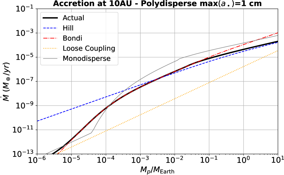
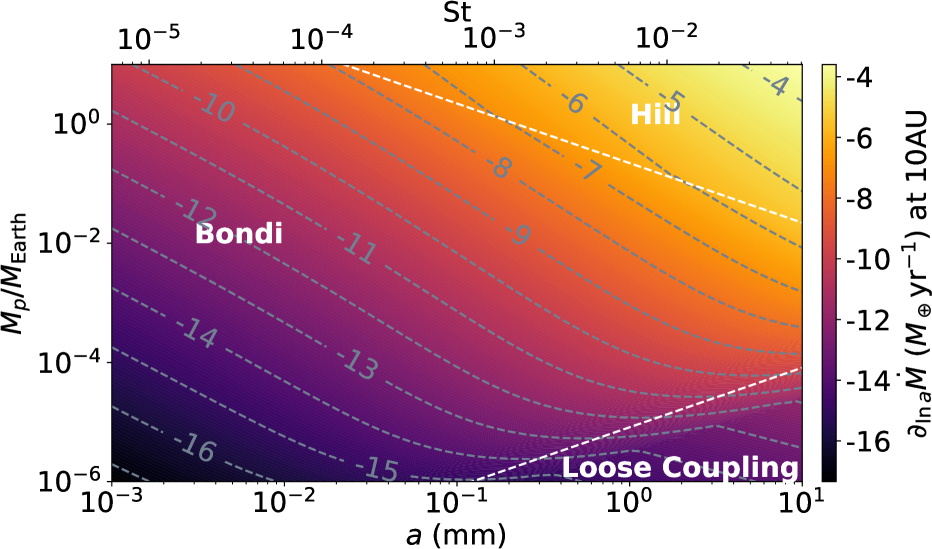
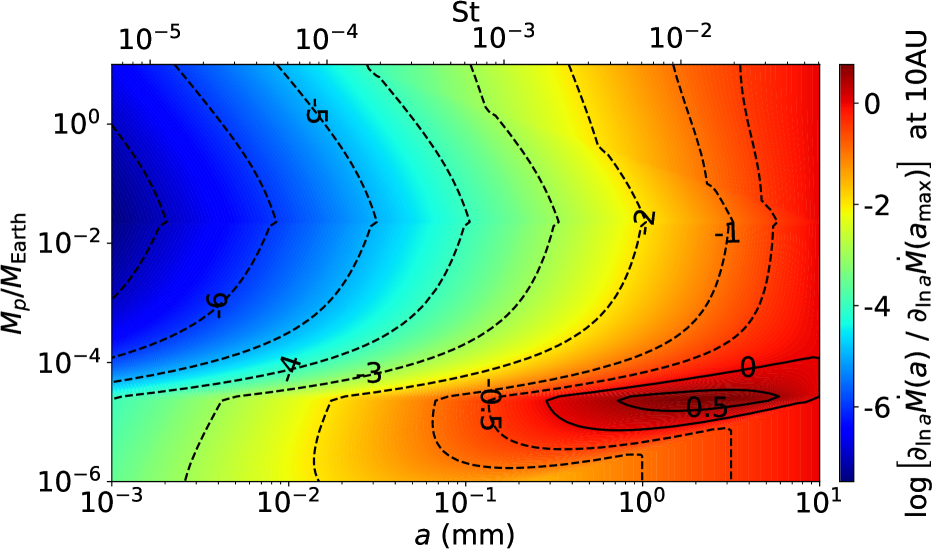
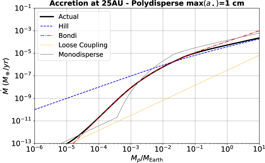
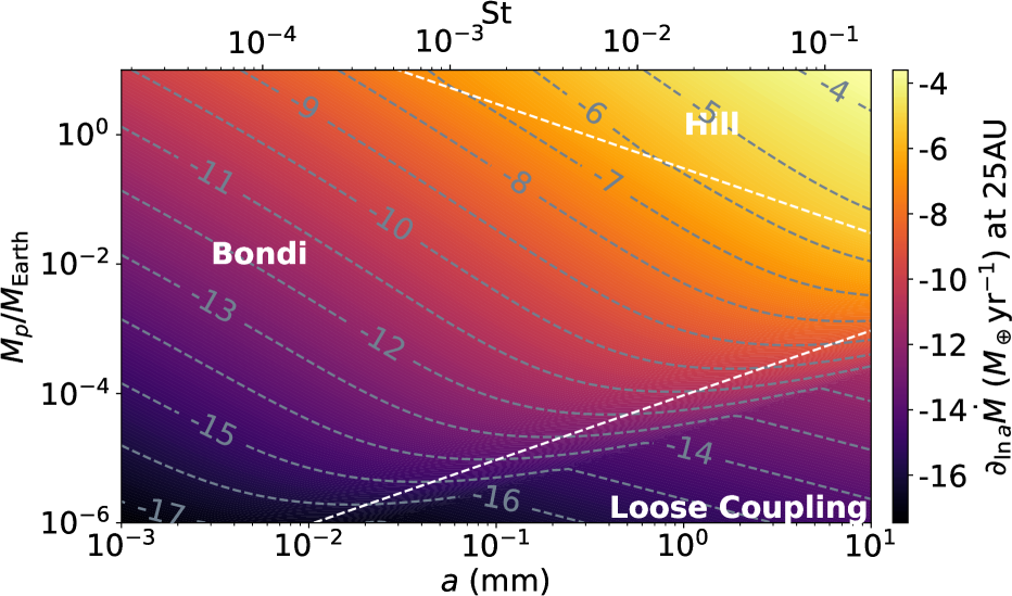
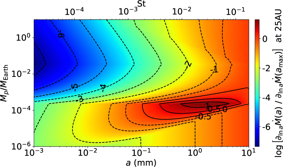
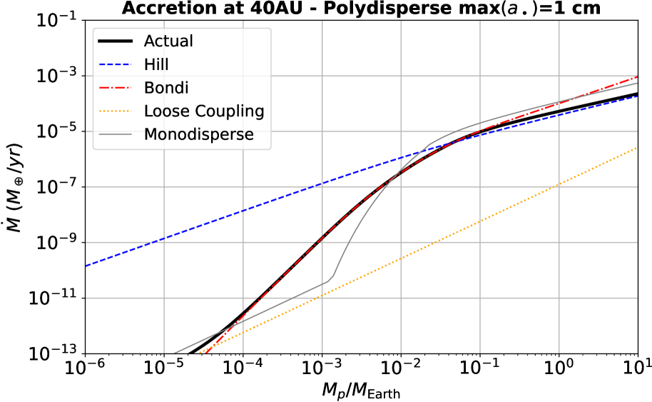
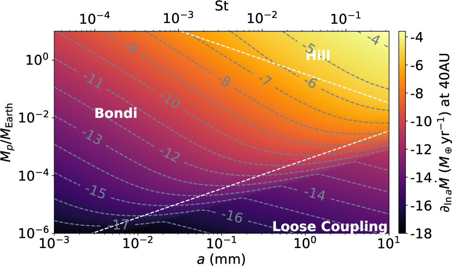
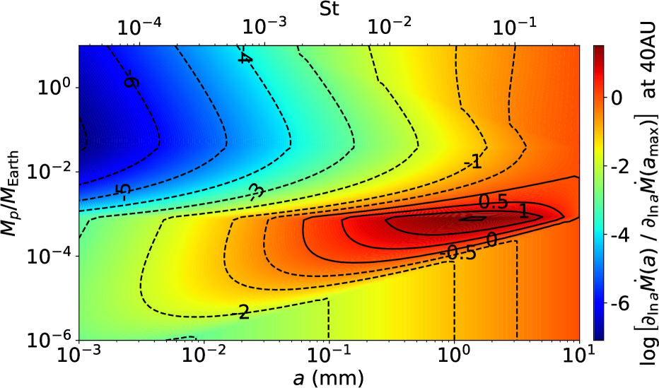
Figure 5: Left: Same as Fig. 3, right plot, but for the density and temperature of Eqs. (23) and (24), Z=0.01, and at different distances. Hill accretion is not much affected by distance, but Bondi accretion becomes increasingly less efficient as distance increases. Yet, the general trend remains, of polydisperse pebble accretion being 1-2 orders of magnitude more efficient than monodisperse at maximum, and showing an earlier onset in mass also by 1-2 orders of magnitude. Middle and Right: same as Fig. 4, at difference distances. The pebble size that maximizes Bondi accretion decreases as distance increases. This has interesting implications, because in the outer disk, the seeds, presumably icy, should accrete small grains, presumably silicates. This implies the possibility a two-mode formation of Kuiper belt objects: icy planetesimal produced by streaming instability of larger grains, followed by pebble accretion of smaller, silicate, grains.

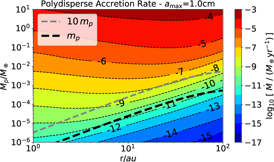
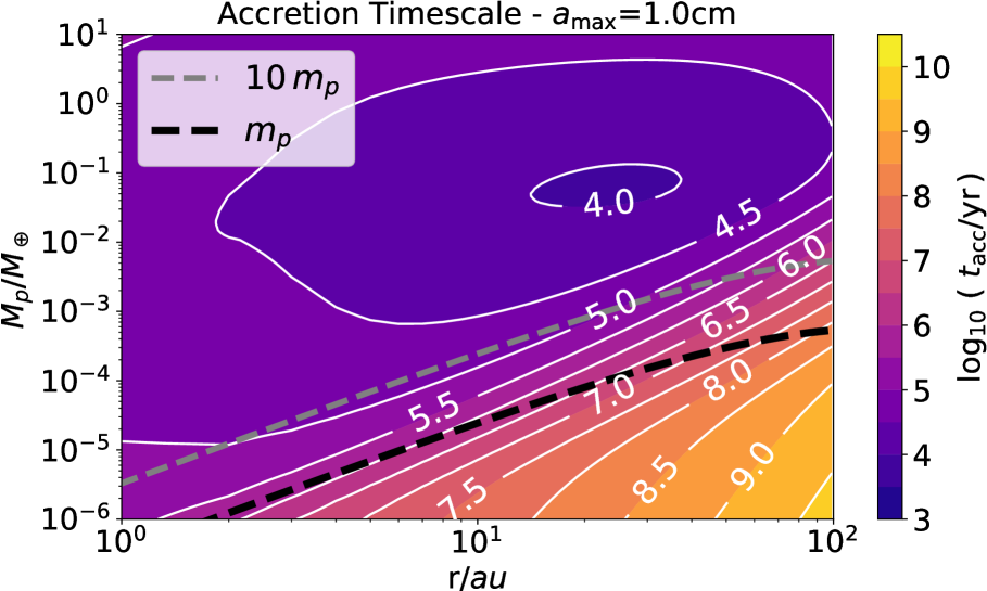
Figure 6: Left: Integrated polydisperse pebble mass accretion rate, as a function of distance. The model uses the density and temperature of Eqs. (23) and (24), Z=0.01, and $\rho_{\bullet}$ constant. The thick black dashed line shows the characteristic size of the planetesimals formed by streaming instability (Liu et al., 2020; Lorek & Johansen, 2022); the grey line represents bodies of 10$\times$ the typical mass. Right: Accretion times $M/\dot{M}$ for the same model. The contour of 6.5 (3Myr) marks the boundary where accretion during the lifetime of the nebula is feasible by pebble accretion, without the need for planetesimal accretion. That contour corresponds to 3 AU, 10 AU, and 30 AU, for $10^{-6}M_{\oplus}$, $2\times 10^{-5}M_{\oplus}$, and $2\times 10^{-4}M_{\oplus}$, respectively. These masses correspond to 100 km radius, $10^{-2}$ and $10^{-1}$ Pluto masses, respectively. The typical products of streaming instability have $<$3 Myr growth times up to 30 AU.

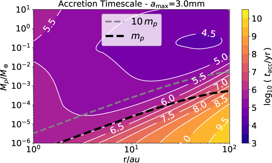
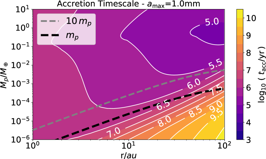
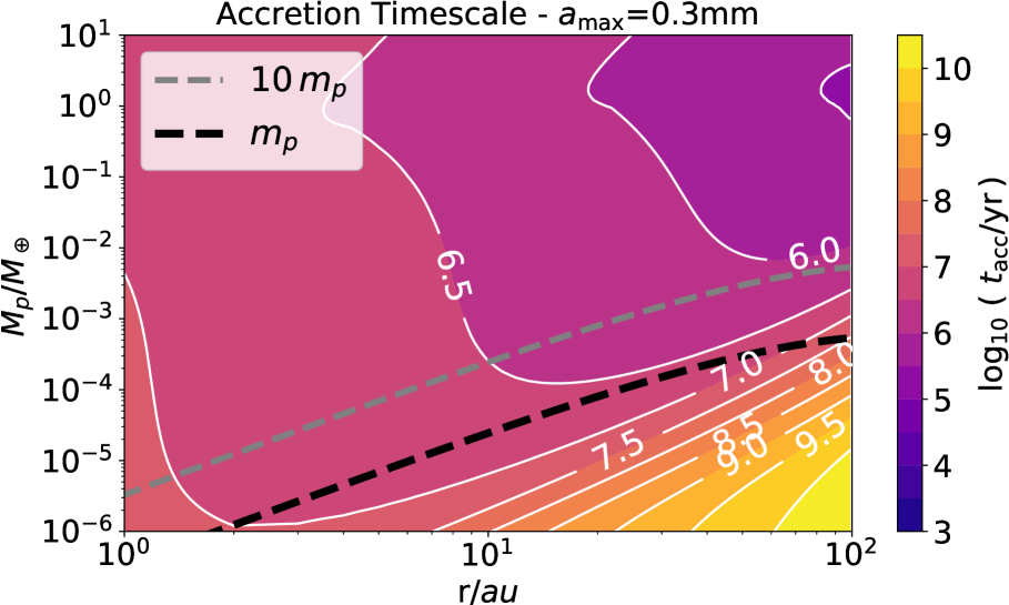
Figure 7: Same as Fig. 6, but exploring the parameter space of maximum grain radius $a_{\rm max}$, from left to right: 3 mm, 1 mm, and 0.3 mm. Upper plots show mass accretion rate, lower plots the accretion times. The trend seen is that Bondi accretion rates decrease with $a_{\rm max}$ for the same seed mass and distance. The contour of 6.5 (3Myr) marks the boundary where accretion during the lifetime of the nebula is feasible by pebble accretion, without the need for planetesimal accretion. This translates into $\approx$ 3 AU for 100  km seeds ($10^{-6}M_{\oplus}$), 10 AU for 0.01 Pluto mass ($2\times 10^{-5}M_{\oplus}$), and up to 30 AU for 0.1 Pluto mass ($2\times 10^{-4}M_{\oplus}$), for the first two models. The typical products of streaming instability grow in Myr timescales except for the last model, of maximum grain size 0.3 mm.

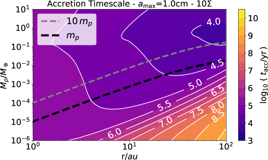
Figure 8: Same as the right panel of Fig. 6, but for 10 times the disk mass. Although the Stokes number decreases for the same particle radius, the increase in dust mass is the dominant effect, and accretion times decrease for the same seed mass and distance. Compared to the lower-mass model, the line of 3 Myr e-folding growth time is pushed to about twice the distance, allowing for pebble accretion on top of 100 km seeds ($10^{-6}M_{\oplus}$) up to 7 AU. 200  km objects ($10^{-5}M_{\oplus}$) can accrete pebbles efficiently up to 30 AU. At 40 AU accretion on 100 km seeds takes over 100 Myr and they should remain planetesimals, consistent with evidence from the Solar System.

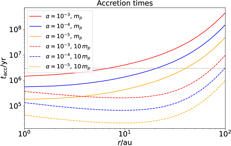
Figure 9: Polydisperse pebble accretion timescales for different $\alpha$ values for the typical masses produced by streaming instability (solid lines), and ten times this mass (dashed lines), taken as proxy for the end of the streaming instability mass function. The grey dotted line marks 3 Myr. For $\alpha=10^{-3}$, the typical seeds only grow within the lifetime of the nebula in the inner solar system, up to $\approx$5-10 AU. For lower turbulence, $\alpha=10^{-5}$, as most pebbles are sedimented, the distance increases to 40 AU.

We explore now the parameter space of stellocentric distance; the results are shown in Fig. 5, showing the accretion rates at 10, 25, and 40 AU (notice also we decreased $a_{\rm max}$ to 1 cm). The left plots show the integrated mass accretion rates $\dot{M}$, the middle plots the distribution $\partial_{\,\ln\,a}\,\dot{M}$, and the right plots the distribution normalized by the accretion rate for $a_{\rm max}$. The Hill accretion rate decreases only slightly with distance for this model, because the drop in $\varOmega$ and $\varSigma_{d}$ with distance is equally compensated by the increase in the Hill radius.

As for the Bondi regime, we see that at the grain size where monodisperse would transition to loosely coupled, polydisperse is still about two orders of magnitude more efficient, over all distances considered. The seed mass for onset of pebble accretion is also pushed down 1 order of magnitude, from $\sim 5\times 10^{-5}$ to $\sim 5\times 10^{-6}M_{\oplus}$ at 10 AU. This is about 100-200 km radius (for internal densities 3.5 and 0.5 g/cm³, respectively), reaching the range where pebble accretion onto the direct products of streaming instability is possible. At 40 AU the onset of pebble accretion is pushed from $\sim 10^{-3}M_{\oplus}$ in monodisperse to $\sim 10^{-4}M_{\oplus}$ in polydisperse. A significant reduction, but still in the mass range of planetary embryos, so planetesimals formed at that distance should remain planetesimals. This is in accordance to the solar system constrain given by the existence of the cold classical Kuiper Belt objects at 40-50 AU, presumably undisturbed planetesimals.

As distance increases, both the accretion rate and the size of the best accreted pebble decreases. While at 10 AU the best accreted size for a $10^{-5}M_{\oplus}$ seed (150-300 km radius) is 1 mm, at 40 AU it decreases to 10 $\mu$m. This has implications for the densities of formed objects if the smaller pebbles have different composition, e.g. the smaller ones being silicate in nature and the larger ones being icy. Then a planetesimal seed will preferentially accrete pebbles of rocky composition until it grows enough in mass to start accreting ices efficiently.

The left panel of Fig. 6 shows the integrated polydisperse pebble accretion rate as a function of distance, from 1 to 100 AU. The mass accretion rate of a $10^{-4}M_{\oplus}$ seed at 20 AU is about $10^{-10}M_{\oplus}{\rm yr}^{-1}$. The thick black dashed line shows the typical mass of objects formed by streaming instability (Liu et al., 2020; Lorek & Johansen, 2022). The thick grey dashed line shows 10 times that mass, proxy for the most massive objects formed directly by streaming instability.

In the right panel we show the accretion time

$$t_{\rm acc}\equiv\frac{M_{p}}{\dot{M}},$$ (54)

along with the same curves for objects formed by streaming instability. The plot shows that a 0.1 Pluto mass ($2\times 10^{-4}M_{\oplus}$) seed has e-folding growth time of 1 Myr at 20 AU, and 10 Myr at 30 AU; that is, a Charon-mass planetary embryo can efficiently increase its mass by Bondi accretion during the lifetime of the disk. This implies that the formation of Pluto in the solar Nebula as far as 30 AU is possible by Bondi accretion of 10-100 $\mu$m grains onto a 0.1 Pluto mass seed.

The plot also shows that up to 20 AU, the objects typically formed by streaming instability (thick black dashed line) have growth times up to 3 Myr, within the lifetime of the nebula. Notice that, in the inner solar system, Bondi accretion on $10^{-6}M_{\oplus}$ seeds ($\approx$ 100 km radius) at 3 Myr timescale is possible up to 3 AU. We conclude that Bondi accretion directly on planetesimals is possible in the inner solar system, dismissing the need for mutual planetesimal collisions as a major contribution to planetary growth.

3.4.1 Effect of maximum grain size

In Fig. 7 we show the model for 3 different maximum grain sizes, from left to right: 3 mm, 1 mm, and 0.3 mm. The main feature is that, as the maximum grain size decreases, the mass accretion rate (accretion time) for given seed mass at a given distance decreases (increases).

The 3 Myr contour reaches $10^{-6}M_{\oplus}$ at 3 AU for $a_{\rm max}$ = 3 mm, $10^{-6}M_{\oplus}$ at 2 AU for 1 mm, and $10^{-4}M_{\oplus}$ at 10 AU for 0.3mm. The conclusion is similar: Myr-timescale Bondi accretion on top of 100 km seeds ($10^{-6}\,M_{\oplus}$) is possible in the inner solar system. Except for the model with $a_{\rm max}=0.3$ mm, the typical products of streaming instability can grow by pebble accretion in 3 Myr timescales.

We calculate also a 10$\times$ more massive model. The higher dust mass also comes with a higher gas mass, and thus a reduction in Stokes number for the same pebble size. It is unclear a priori which effect dominates. In Fig. 8 we show the formation times for the model, using $a_{\rm max}=1\,$cm. The formation times are overall shorter compared to the right panel of Fig. 6, pushing the 3 Myr e-folding contour to double the distance vis-à-vis the lower mass model (7 AU for 100 km, 30 AU for $10^{-2}$ Pluto mass, and 60 AU for $10^{-1}$ Pluto mass). Even at this higher mass model, a 100 km seed has an e-folding growth time of over 100 Myr at 40 AU, and should remain planetesimals, as expected.

3.4.2 Effect of sedimentation

In Fig. 9 we show the e-folding growth times for the planetary seeds formed by streaming instability (typical objects and most massive objects), as a function of the turbulent viscosity parameter $\alpha$. Its function in the model is only on how it influences sedimentation. The grey dotted line in the plot marks the threshold of 3 Myr. For moderately high turbulence ($\alpha=10^{-3}$), the typical seeds have longer growth times than 3 Myr already beyond 6 AU. For lower turbulence, $\alpha=10^{-5}$, as most pebbles are sedimented, the distance where growth occurs within 3 Myr increases to 40 AU. The most massive objects, well into the Bondi regime, all have fast growth times.

4 Analytical solutions

In this section we derive the analytical solutions in the relevant limits of 2D Hill accretion and 3D Bondi accretion. In a polydisperse distribution, the pebble scale height is a function of pebble radius, so the pebbles are not necessarily all in the 2D regime or all in the 3D regime. Also, because the transitions between loosely coupled and Bondi, and from Bondi to Hill are St-dependent, the pebbles are not all in the same regime of accretion either.

Yet, in practice these limits still yield reasonably accurate accretion rates. Because the distribution is top heavy, the 2D Hill regime is applicable for large seed masses, that are accreting in this regime the biggest pebbles, which are responsible for most of the mass accretion rate. The 3D Bondi regime is applicable as long as $R_{\rm acc}<2H_{d}$ (Eq. 28), which solving for mass yields

$$M_{p}<\frac{\Delta v\varOmega H_{g}^{2}\alpha}{G\mathrm{St}\left(\mathrm{St}+\alpha\right)}.$$ (55)

Normalizing by the transition mass $M_{t}$, we find

$$\frac{M_{p}}{M_{t}}\lesssim\frac{\alpha}{h^{2}\mathrm{St}\left(\mathrm{St}+\alpha\right)},$$ (56)

where $h\equiv H_{g}/r$ is the disk aspect ratio. For $\alpha\sim 10^{-4}$ and $h\sim 10^{-2}$, 3D Bondi accretion should apply close to the transition mass, except for big enough pebbles, as expected, because these are too sedimented. Yet, as we have established, these pebbles contribute poorly to the mass accretion rate. For particles of $\tau_{f}=t_{B}$, and assuming $\mathrm{St}\gg\alpha$, we find

$$\frac{M_{p}}{M_{t}}\lesssim\left(\frac{\alpha}{h^{2}}\right)^{1/3},$$ (57)

i.e., within the expected ranges of $\alpha$ and $h$, the seed mass for which $\tau_{f}=t_{B}$ is within a factor of order unity from the transition mass. We conclude that a 3D approximation for the Bondi regime should lead to acceptable results.

We work now the analytical expressions in these limits.

4.1 Analytical Polydisperse 2D Hill accretion

We can integrate the polydisperse Hill regime analytically in the 2D limit by generalizing Eq. (30) with $\varSigma_{d}$ given by Eq. (26)

$$\dot{M}_{\rm 2D,Hill}=2\times 10^{2/3}\varOmega R_{H}^{2}\int_{0}^{a_{\rm max}}\mathrm{St}(a)^{2/3}\,m(a)\,W(a)\,da.$$ (58)

Given the scalings $\mathrm{St}\propto a^{1-q}$, $m\propto a^{3-q}$, and $W\propto a^{-k}$, the dependency of the integrand of Eq. (58) on $a$ is

$$\frac{\partial\dot{M}(a)}{\partial a}_{\rm 2D,Hill}\propto a^{(11-5q-3k)/3}$$ (59)

Integrating it in $a$, we find the exact solution

$$\dot{M}_{\rm 2D,Hill}=\frac{6(1-p)}{14-5q-3k}\left(\frac{\mathrm{St}_{\rm max}}{0.1}\right)^{2/3}\varOmega\,R_{H}^{2}\,Z\,\varSigma_{g}.$$ (60)

Eq. (60) differs from the monodisperse case (Eq. 30) by an efficiency factor

$$\left(\frac{\dot{M}_{\rm poly}}{\dot{M}_{\rm mono}}\right)_{\rm 2D,Hill}=\frac{3(1-p)}{14-5q-3k}\left(\frac{\mathrm{St}_{\rm max}}{\mathrm{St}}\right)^{2/3}.$$ (61)

For MRN $(k=3.5)$, $q=0$, and $\mathrm{St}=\mathrm{St}_{\rm max}$, this yields

$$\left(\frac{\dot{M}_{\rm poly}}{\dot{M}_{\rm mono}}\right)_{\rm 2D,Hill}^{k=3.5,q=0}=\frac{3}{7},$$ (62)

that is, about 43% of the monodisperse. Deviations from this number are due to not all pebbles being in the 2D Hill regime. For large enough seed mass, the deviations should be small, as indeed it is seen in the plots of Figs. 3 and 5.

4.2 Analytical Polydisperse 3D Bondi accretion

The Bondi accretion in the 3D regime limit is found by generalizing Eq. (29) with $\rho_{d0}$ given by Eq. (39)

$$\dot{M}_{\rm 3D,Bondi} = \frac{4\pi R_{B}\Delta v^{2}}{\varOmega}\times$$

$$\int_{0}^{a_{\rm max}}\mathrm{St}\ e^{-2\psi}m(a)f(a)\left[1+2\left(\mathrm{St}\frac{\varOmega R_{B}}{\Delta v}\right)^{1/2}e^{-\psi}\right]da,$$

where we use the shorthand notation

$$\psi\equiv\chi[\mathrm{St}/(\varOmega t_{p})]^{\gamma}.$$ (64)

We will split Eq. (LABEL:eq:3dbondipolyint) into two integrals

$$\dot{M}_{\rm 3D,Bondi} = \frac{4\pi R_{B}\Delta v^{2}}{\varOmega}\left[\int_{0}^{a_{\rm max}}e^{-2\psi}\ \mathrm{St}\ m(a)\ f(a)\ da\right.$$

$$+ \left.2\left(\frac{\varOmega R_{B}}{\Delta v}\right)^{1/2}\int_{0}^{a_{\rm max}}e^{-3\psi}\ \mathrm{St}^{3/2}\ m(a)\ f(a)\ da\right].$$

The function $f(a)$ has a dependency on $\sqrt{1+\mathrm{St}/\alpha}$, which makes these functions non-integrable sauf specific cases. We will thus use the following approximation, valid at $x\rightarrow 0$ and $x\rightarrow\infty$

$$\sqrt{1+x}\approx 1+\sqrt{x}.$$ (66)

While the error incurred with this approximation at $x\approx 1$ can be large, we are interested in the definite integral from 0 to $x_{\rm max}$. In this case, the error decreases if the range of integration is large enough, tending to zero for $x_{\rm max}\rightarrow\infty$, as shown in Fig. 10. Confident in the accuracy of Eq. (66), we write the approximate solution

$$\dot{M}_{\rm 3D,Bondi} \approx \frac{3(1-p)Z\varSigma_{g}R_{B}\Delta v^{2}}{\sqrt{2\pi}H_{g}\varOmega\rho_{\bullet}^{(0)}a_{\rm max}^{4-k}}\times$$ (67)

$$\left[\int_{0}^{a_{\rm max}}e^{-2\psi}\ \mathrm{St}\ m(a)\ a^{-k}da\right.$$

$$+ \alpha^{-1/2}\int_{0}^{a_{\rm max}}e^{-2\psi}\ \mathrm{St}^{3/2}\ m(a)\ a^{-k}da$$

$$+ 2\left(\frac{\varOmega R_{B}}{\Delta v}\right)^{1/2}\int_{0}^{a_{\rm max}}e^{-3\psi}\ \mathrm{St}^{3/2}\ m(a)\ a^{-k}da$$

$$+ \left.2\left(\frac{\varOmega R_{B}}{\alpha\Delta v}\right)^{1/2}\int_{0}^{a_{\rm max}}e^{-3\psi}\ \mathrm{St}^{2}\ m(a)\ a^{-k}da\right].$$

The four integrals are of the form below, for which there is an analytical solution in terms of lower incomplete gamma functions

$$\int_{0}^{a_{\rm max}}e^{-ja^{s}}a^{b}da=\frac{\gamma_{l}\left(\frac{b+1}{s},ja_{\rm max}^{s}\right)}{sj^{(b+1)/s}}.$$ (68)

We thus write the solution of Eq. (67)

$$\dot{M}_{\rm 3D,Bondi} \approx C_{1}\frac{\gamma_{l}\left(\frac{b_{1}+1}{s},j_{1}a_{\rm max}^{s}\right)}{sj_{1}^{(b_{1}+1)/s}}+C_{2}\frac{\gamma_{l}\left(\frac{b_{2}+1}{s},j_{2}a_{\rm max}^{s}\right)}{sj_{2}^{(b_{2}+1)/s}}+$$ (69)

$$C_{3}\frac{\gamma_{l}\left(\frac{b_{3}+1}{s},j_{3}a_{\rm max}^{s}\right)}{sj_{3}^{(b_{3}+1)/s}}+C_{4}\frac{\gamma_{l}\left(\frac{b_{4}+1}{s},j_{4}a_{\rm max}^{s}\right)}{sj_{4}^{(b_{4}+1)/s}},$$

where the coefficients are

$$s = \gamma(1-q)$$ (70)

$$b_{1} = 4-2q-k$$ (71)

$$b_{2}=b_{3} = (9-5q-2k)/2$$ (72)

$$b_{4} = 5-3q-k$$ (73)

$$\mathrm{St}^{\prime} = \frac{\pi}{2\varSigma_{g}}\rho_{\bullet}^{(0)}a_{\rm max}^{q}$$ (74)

$$j^{\prime} = \chi\left(\frac{\mathrm{St}^{\prime}}{\varOmega t_{p}}\right)^{\gamma}$$ (75)

$$j_{1}=j_{2} = 2j^{\prime}$$ (76)

$$j_{3}=j_{4} = 3j^{\prime}$$ (77)

$$m^{\prime} = \frac{4\pi}{3}\rho_{\bullet}^{(0)}a_{\rm max}^{q}$$ (78)

$$K = \frac{3(1-p)Z\varSigma_{g}R_{B}\Delta v^{2}}{\sqrt{2\pi}H_{g}\varOmega\rho_{\bullet}^{(0)}a_{\rm max}^{4-k}}$$ (79)

$$C_{1} = K\mathrm{St}^{\prime}m^{\prime}$$ (80)

$$C_{2} = K\mathrm{St}^{\prime 3/2}m^{\prime}\alpha^{-1/2}$$ (81)

$$C_{3} = 2K\mathrm{St}^{\prime 3/2}m^{\prime}\left(\frac{\varOmega R_{B}}{\Delta v}\right)^{1/2}$$ (82)

$$C_{4} = 2K\mathrm{St}^{\prime 2}m^{\prime}\left(\frac{\varOmega R_{B}}{\alpha\Delta v}\right)^{1/2}$$ (83)

Fig. 11 shows that the agreement between the numerical integration of Eq. (37) and the analytical solutions (Eq. (60) and Eq. (69)) is excellent in the range of validity. Having Eq. (60) and Eq. (69) as analytical expressions is of great interest for future studies including pebble accretion analytically, instead of having to integrate the mass accretion rates numerically with the particle size distributions.

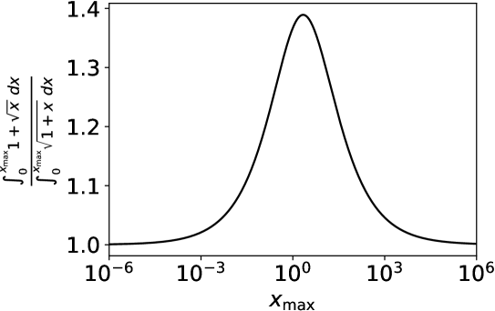
Figure 10: Approximating $\sqrt{1+x}$ in by $1+\sqrt{x}$ (the asymptotic expansion for $x\rightarrow 0$ and $x\rightarrow\infty$), to make the sedimented midplane distribution integrable analytically. As long as the function is integrated to a large value of $x_{\rm max}$, the error incurred is small.

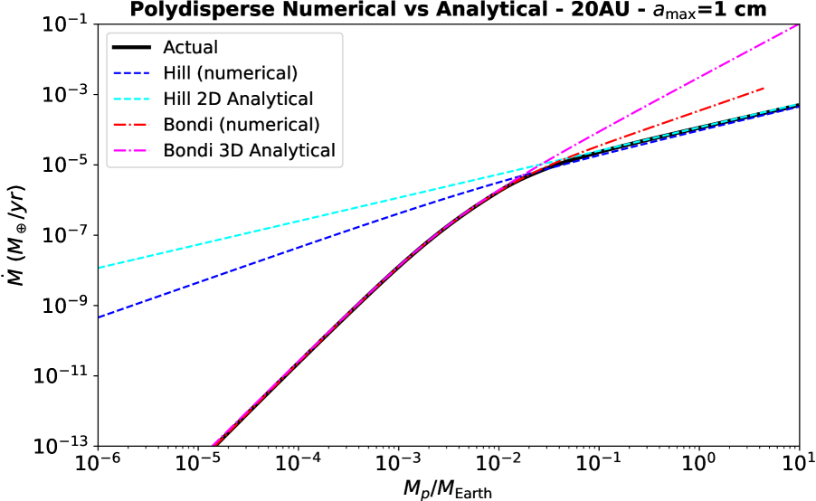
Figure 11: Agreement between the numerically calculated polydisperse pebble accretion rate and the analytical solutions for 2D Hill accretion Eq. (60) and 3D Bondi accretion Eq. (69). While the Hill solution is exact, the Bondi solution is approximate. Yet, the agreement seen is excellent, because the best accreted pebbles in this regime are in the 3D range.

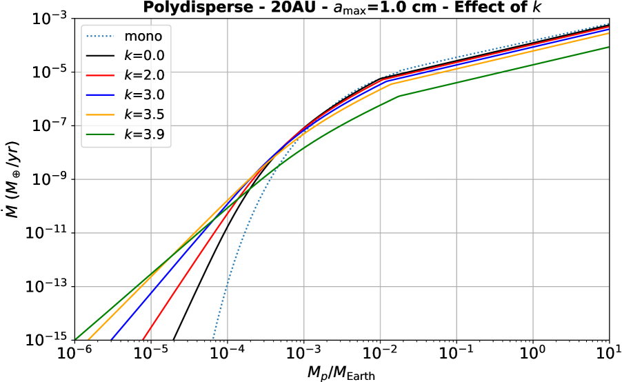
Figure 12: Effect of varying the slope $k$ of the grain size distribution. The Hill regime is relatively insensitive to $k$, as this regime is dominated by the largest grains. For Bondi accretion, the mass accretion rates increase significantly as the slope steepens.

5 Effect of slope $k$ of grain size distribution

So far we have considered only the MRN value for the index $k$ of the grain size distribution (Mathis et al., 1977), but this index should depend on the collisional evolution, velocities, and material strength of the pebbles (Kobayashi & Tanaka, 2010; Kobayashi et al., 2016). Having found the analytical solution for the accretion rates, we can more easily determine the impact of varying this parameter, which we show in Fig. 12. As the slope steepens, the mass accretion rate decreases in the Hill regime. Compared to monodisperse, the effect is small, but accelerates as $k$ approaches 4. This insensitivity is expected, as the Hill regime is dominated by the larger grains. The effect on mass accretion rate is more pronounced for the Bondi regime, as expected, as the amount of mass in different grain sizes more strongly affects this accretion regime. As the slope steepens and more mass is made available in small grain sizes, the accretion rates onto smaller planetesimal seeds increases, although the effect is nonlinear.

6 Limitations

We are limited in this work by the vast expanses of the parameter space and by the circular restricted 3-body problem solution that forms for the underlying assumption of the gas and pebble flow. While the former would be a valiant endeavour, it is not the scope of this work to derive results applicable to all possible situations, but to derive the model in first place. As such, we kept our equations general in metallicity, internal density, and grain size distribution, but apply it mostly for $Z=0.01$, $\rho_{\bullet}^{(0)}=3.5$ g cm^-3, $q=0$. These parameters will vary with dust drift (lower the metallicity), composition (varying the internal density if ices or silicates), and porosity.

As for going beyond the circular restricted 3-body problem, recently the impact of the gravity of the planetary seed on the accretion flow has been calculated from hydrodynamical simulations (Okamura & Kobayashi, 2021), for the Hill regime (Kuwahara & Kurokawa, 2020a) and for the Bondi regime (Kuwahara & Kurokawa, 2020b). In the Bondi regime, the trajectories are modified for $\mathrm{St}\lesssim 10^{-3}$, with the gas flow reducing the accretion rate. Thus, Eq. (45) is overestimated for small $\mathrm{St}$. We find that the best accreted pebbles, that give the bulk of the boost in Bondi accretion, are slightly above the $\mathrm{St}\sim 10^{-3}$ transition found by (Kuwahara & Kurokawa, 2020b); as such, this aspect of our results are not severely affected by the planet-induced flow.

7 Conclusion

In this paper, we worked out the theory of polydisperse pebble accretion, finding analytical solutions when possible. Our main findings are as follows:

• We find that polydisperse Bondi accretion is 1-2 orders of magnitudes more efficient than in the monodisperse case, This is because the best-accreted pebbles in the Bondi regime are those of friction time similar to Bondi time, not the largest pebbles present. The large pebbles, although dominating the mass budget, are weakly coupled across the Bondi radius and thus accrete poorly. The pebbles that are optimal for Bondi accretion may contribute less to the mass budget, but their enhanced accretion significantly impacts the mass accretion rate.

• The onset of polydisperse pebble accretion is extended by 1-2 orders of magnitude lower in mass compared to monodisperse, for the same reason. The onset of pebble accretion with Myr-timescales reaches 100-350 km sized objects depending on stellocentric distances and disk model. For the model considered, Bondi accretion on Myr timescales, within the lifetime of the disk, is possible on top of $10^{-6}M_{\oplus}$ (100 km) seeds up to 4 AU, on top of $10^{-5}M_{\oplus}$ (200 km) seeds up to 10 AU, and on $10^{-4}M_{\oplus}$ (350 km) seeds up to 30 AU. A model 10 times more massive doubles these distances.

• In all models considered, at 40 AU a 100 km seed has growth time over 100 Myr, and should thus remain as planetesimals, in accordance with the existence of the cold classical Kuiper Belt population, presumably undisturbed planetesimals.

• We find the analytical solution of the stratification integral, and thus the exact solution for the 3D-2D transition (Eq. 35),

• We find analytical solutions for the polydisperse 2D Hill (Eq. 60) and 3D Bondi regime (Eq. 69). For the MRN distribution, the Hill accretion is a factor 3/7 (about 42%) as efficient in polydisperse than monodisperse.

The fact that Myr-growth timescales, within the lifetime of the disk, is possible for polydisperse pebble accretion onto 100-350 km seeds over a significant range of the parameter space, has significant implications. This mass range overlaps with the high mass end of the planetesimal initial mass function (Johansen et al., 2015; Schäfer et al., 2017; Li et al., 2019), and thus pebble accretion is possible directly following formation by streaming instability, removing the need for planetesimal accretion. This conclusion is supported by the lack of of craters generated by 1-2 km on Pluto (Singer et al., 2019), and recent findings by Lorek & Johansen (2022) that planetesimal accretion are not able to sustain accretion rates beyond 5 AU.

While we do most of our numerical solutions with constant $\rho_{\bullet}$, we keep the analytical solutions general for varying this parameter, expecting that smaller pebbles should be of lower density, and the bigger pebbles of higher density, reflecting different compositions (Morales et al., 2016). We notice that as the distance increases, the pebble size that maximizes pebble accretion is increasingly smaller. This implies the possibility of a two-mode formation of Kuiper belt objects: streaming instability of the largest pebbles forming icy objects of the order of $\gtrsim$ 100 km in diameter, followed by pebble accretion leading to objects of the order of 1000 km, where silicates are incorporated mostly at the pebble accretion stage, due to their low Stokes number. This scenario would lead to a different composition for the smaller objects, mostly formed by ice streaming instability, and the larger objects, grown by ice and silicate pebble accretion on top of the icy planetesimal seeds. A continuum of rock-to-ice fraction should be produced. Indeed a trend is clear in the Kuiper belt, of constant density around 0.5 g cm^-3 for the smaller objects (diameter less than 500 km), and increasing for larger objects (Brown, 2012; Grundy et al., 2015; McKinnon et al., 2017). We will explore how our findings in this paper can reproduce this result in a future work.

References

- Andama et al. (2022) Andama, G., Ndugu, N., Anguma, S. K., & Jurua, E. 2022, MNRAS, 510, 1298
- Appelgren et al. (2020) Appelgren, J., Lambrechts, M., & Johansen, A. 2020, A&A, 638, A156
- Birnstiel et al. (2012) Birnstiel, T., Klahr, H., & Ercolano, B. 2012, A&A, 539, A148
- Bitsch et al. (2019a) Bitsch, B., Izidoro, A., Johansen, A., Raymond, S. N., Morbidelli, A., Lambrechts, M., & Jacobson, S. A. 2019a, arXiv e-prints
- Bitsch et al. (2019b) Bitsch, B., Raymond, S. N., & Izidoro, A. 2019b, A&A, 624, A109
- Blum & Wurm (2008) Blum, J., & Wurm, G. 2008, ARA&A, 46, 21
- Bondi & Hoyle (1944) Bondi, H., & Hoyle, F. 1944, MNRAS, 104, 273
- Brauer et al. (2008) Brauer, F., Dullemond, C. P., & Henning, T. 2008, A&A, 480, 859
- Brown (2012) Brown, M. E. 2012, Annual Review of Earth and Planetary Sciences, 40, 467
- Carrera et al. (2015) Carrera, D., Johansen, A., & Davies, M. B. 2015, A&A, 579, A43
- Chen & Lin (2020) Chen, K., & Lin, M.-K. 2020, ApJ, 891, 132
- Drazkowska et al. (2022) Drazkowska, J., Bitsch, B., Lambrechts, M., Mulders, G. D., Harsono, D., Vazan, A., Liu, B., Ormel, C. W., Kretke, K., & Morbidelli, A. 2022, arXiv e-prints, arXiv:2203.09759
- Dr\każkowska et al. (2021) Dr\każkowska, J., Stammler, S. M., & Birnstiel, T. 2021, A&A, 647, A15
- Dubrulle et al. (1995) Dubrulle, B., Morfill, G., & Sterzik, M. 1995, Icarus, 114, 237
- Dullemond & Dominik (2005) Dullemond, C. P., & Dominik, C. 2005, A&A, 434, 971
- Flock & Mignone (2021) Flock, M., & Mignone, A. 2021, A&A, 650, A119
- Geretshauser et al. (2010) Geretshauser, R. J., Speith, R., Güttler, C., Krause, M., & Blum, J. 2010, A&A, 513, A58
- Grundy et al. (2015) Grundy, W. M., Porter, S. B., Benecchi, S. D., Roe, H. G., Noll, K. S., Trujillo, C. A., Thirouin, A., Stansberry, J. A., Barker, E., & Levison, H. F. 2015, Icarus, 257, 130
- Guilera et al. (2020) Guilera, O. M., Sándor, Z., Ronco, M. P., Venturini, J., & Miller Bertolami, M. M. 2020, A&A, 642, A140
- Güttler et al. (2010) Güttler, C., Blum, J., Zsom, A., Ormel, C. W., & Dullemond, C. P. 2010, A&A, 513, A56
- Güttler et al. (2009) Güttler, C., Krause, M., Geretshauser, R. J., Speith, R., & Blum, J. 2009, ApJ, 701, 130
- Hirashita & Kobayashi (2013) Hirashita, H., & Kobayashi, H. 2013, Earth, Planets and Space, 65, 1083
- Hoyle & Lyttleton (1939) Hoyle, F., & Lyttleton, R. A. 1939, Proceedings of the Cambridge Philosophical Society, 35, 405
- Ida et al. (2016) Ida, S., Guillot, T., & Morbidelli, A. 2016, A&A, 591, A72
- Izidoro et al. (2021) Izidoro, A., Bitsch, B., Raymond, S. N., Johansen, A., Morbidelli, A., Lambrechts, M., & Jacobson, S. A. 2021, A&A, 650, A152
- Johansen & Bitsch (2019) Johansen, A., & Bitsch, B. 2019, A&A, 631, A70
- Johansen & Lacerda (2010) Johansen, A., & Lacerda, P. 2010, MNRAS, 404, 475
- Johansen & Lambrechts (2017) Johansen, A., & Lambrechts, M. 2017, Annual Review of Earth and Planetary Sciences, 45, 359
- Johansen et al. (2015) Johansen, A., Mac Low, M.-M., Lacerda, P., & Bizzarro, M. 2015, Science Advances, 1, 1500109
- Johansen et al. (2007) Johansen, A., Oishi, J. S., Mac Low, M.-M., Klahr, H., Henning, T., & Youdin, A. 2007, Nature, 448, 1022
- Johansen et al. (2021) Johansen, A., Ronnet, T., Bizzarro, M., Schiller, M., Lambrechts, M., Nordlund, Å., & Lammer, H. 2021, Science Advances, 7, eabc0444
- Johansen & Youdin (2007) Johansen, A., & Youdin, A. 2007, ApJ, 662, 627
- Klahr & Schreiber (2021) Klahr, H., & Schreiber, A. 2021, ApJ, 911, 9
- Klahr & Henning (1997) Klahr, H. H., & Henning, T. 1997, Icarus, 128, 213
- Kobayashi & Tanaka (2010) Kobayashi, H., & Tanaka, H. 2010, Icarus, 206, 735
- Kobayashi et al. (2016) Kobayashi, H., Tanaka, H., & Okuzumi, S. 2016, ApJ, 817, 105
- Kowalik et al. (2013) Kowalik, K., Hanasz, M., Wóltański, D., & Gawryszczak, A. 2013, MNRAS, 434, 1460
- Krapp et al. (2019) Krapp, L., Benítez-Llambay, P., Gressel, O., & Pessah, M. E. 2019, ApJL, 878, L30
- Krijt et al. (2015) Krijt, S., Ormel, C. W., Dominik, C., & Tielens, A. G. G. M. 2015, A&A, 574, A83
- Kusaka et al. (1970) Kusaka, T., Nakano, T., & Hayashi, C. 1970, Progress of Theoretical Physics, 44, 1580
- Kuwahara & Kurokawa (2020a) Kuwahara, A., & Kurokawa, H. 2020a, A&A, 633, A81
- Kuwahara & Kurokawa (2020b) —. 2020b, A&A, 643, A21
- Lambrechts & Johansen (2012) Lambrechts, M., & Johansen, A. 2012, A&A, 544, A32
- Lambrechts & Johansen (2014) —. 2014, A&A, 572, A107
- Lambrechts et al. (2014) Lambrechts, M., Johansen, A., & Morbidelli, A. 2014, A&A, 572, A35
- Lambrechts et al. (2019) Lambrechts, M., Morbidelli, A., Jacobson, S. A., Johansen, A., Bitsch, B., Izidoro, A., & Raymond, S. N. 2019, arXiv e-prints
- Li & Youdin (2021) Li, R., & Youdin, A. N. 2021, ApJ, 919, 107
- Li et al. (2019) Li, R., Youdin, A. N., & Simon, J. B. 2019, ApJ, 885, 69
- Lin (2021) Lin, M.-K. 2021, ApJ, 907, 64
- Liu et al. (2020) Liu, B., Lambrechts, M., Johansen, A., Pascucci, I., & Henning, T. 2020, A&A, 638, A88
- Lorek & Johansen (2022) Lorek, S., & Johansen, A. 2022, arXiv e-prints, arXiv:2208.01902
- Lynden-Bell & Pringle (1974) Lynden-Bell, D., & Pringle, J. E. 1974, MNRAS, 168, 603
- Lyra et al. (2008) Lyra, W., Johansen, A., Klahr, H., & Piskunov, N. 2008, A&A, 491, L41
- Lyra & Kuchner (2013) Lyra, W., & Kuchner, M. 2013, Nature, 499, 184
- Lyra & Lin (2013) Lyra, W., & Lin, M.-K. 2013, ApJ, 775, 17
- Mathis et al. (1977) Mathis, J. S., Rumpl, W., & Nordsieck, K. H. 1977, ApJ, 217, 425
- McKinnon et al. (2017) McKinnon, W. B., Stern, S. A., Weaver, H. A., Nimmo, F., Bierson, C. J., Grundy, W. M., Cook, J. C., Cruikshank, D. P., Parker, A. H., Moore, J. M., Spencer, J. R., Young, L. A., Olkin, C. B., Ennico Smith, K., New Horizons Geology, G., Imaging, & Composition Theme Teams. 2017, Icarus, 287, 2
- McNally et al. (2021) McNally, C. P., Lovascio, F., & Paardekooper, S.-J. 2021, MNRAS, 502, 1469
- Morales et al. (2016) Morales, F. Y., Bryden, G., Werner, M. W., & Stapelfeldt, K. R. 2016, ApJ, 831, 97
- Nakagawa et al. (1981) Nakagawa, Y., Nakazawa, K., & Hayashi, C. 1981, Icarus, 45, 517
- Nesvorný et al. (2019) Nesvorný, D., Li, R., Youdin, A. N., Simon, J. B., & Grundy, W. M. 2019, Nature Astronomy, 349
- Okamura & Kobayashi (2021) Okamura, T., & Kobayashi, H. 2021, ApJ, 916, 109
- Ormel (2017) Ormel, C. W. 2017, in Astrophysics and Space Science Library, Vol. 445, Astrophysics and Space Science Library, ed. M. Pessah & O. Gressel, 197
- Ormel & Klahr (2010) Ormel, C. W., & Klahr, H. H. 2010, A&A, 520, A43
- Paardekooper et al. (2020) Paardekooper, S.-J., McNally, C. P., & Lovascio, F. 2020, MNRAS, 499, 4223
- Pollack et al. (1994) Pollack, J. B., Hollenbach, D., Beckwith, S., Simonelli, D. P., Roush, T., & Fong, W. 1994, ApJ, 421, 615
- Raymond et al. (2004) Raymond, S. N., Quinn, T., & Lunine, J. I. 2004, Icarus, 168, 1
- Safronov (1972) Safronov, V. S. 1972, Evolution of the protoplanetary cloud and formation of the earth and planets.
- Schäfer et al. (2020) Schäfer, U., Johansen, A., & Banerjee, R. 2020, A&A, 635, A190
- Schäfer et al. (2017) Schäfer, U., Yang, C.-C., & Johansen, A. 2017, A&A, 597, A69
- Schaffer et al. (2018) Schaffer, N., Yang, C.-C., & Johansen, A. 2018, A&A, 618, A75
- Shakura & Sunyaev (1973) Shakura, N. I., & Sunyaev, R. A. 1973, A&A, 24, 337
- Simon et al. (2016) Simon, M. N., Pascucci, I., Edwards, S., Feng, W., Gorti, U., Hollenbach, D., Rigliaco, E., & Keane, J. T. 2016, ApJ, 831, 169
- Singer et al. (2019) Singer, K. N., McKinnon, W. B., Gladman, B., Greenstreet, S., Bierhaus, E. B., Stern, S. A., Parker, A. H., Robbins, S. J., Schenk, P. M., Grundy, W. M., Bray, V. J., Beyer, R. A., Binzel, R. P., Weaver, H. A., Young, L. A., Spencer, J. R., Kavelaars, J. J., Moore, J. M., Zangari, A. M., Olkin, C. B., Lauer, T. R., Lisse, C. M., Ennico, K., New Horizons Geology, G., Team, I. S. T., New Horizons Surface Composition Science Theme Team, & New Horizons Ralph and LORRI Teams. 2019, Science, 363, 955
- Squire & Hopkins (2020) Squire, J., & Hopkins, P. F. 2020, MNRAS, 498, 1239
- Suyama et al. (2008) Suyama, T., Wada, K., & Tanaka, H. 2008, ApJ, 684, 1310
- Suyama et al. (2012) Suyama, T., Wada, K., Tanaka, H., & Okuzumi, S. 2012, ApJ, 753, 115
- Thommes et al. (2003) Thommes, E. W., Duncan, M. J., & Levison, H. F. 2003, Icarus, 161, 431
- Tominaga et al. (2021) Tominaga, R. T., Inutsuka, S.-i., & Kobayashi, H. 2021, ApJ, 923, 34
- Venturini et al. (2020) Venturini, J., Guilera, O. M., Ronco, M. P., & Mordasini, C. 2020, A&A, 644, A174
- Visser et al. (2021) Visser, R. G., Dr\każkowska, J., & Dominik, C. 2021, A&A, 647, A126
- Yang & Johansen (2014) Yang, C.-C., & Johansen, A. 2014, ApJ, 792, 86
- Yang et al. (2017) Yang, C. C., Johansen, A., & Carrera, D. 2017, A&A, 606, A80
- Yang et al. (2018) Yang, C.-C., Mac Low, M.-M., & Johansen, A. 2018, ApJ, 868, 27
- Yang & Zhu (2021) Yang, C.-C., & Zhu, Z. 2021, MNRAS, 508, 5538
- Youdin & Johansen (2007) Youdin, A., & Johansen, A. 2007, ApJ, 662, 613
- Youdin & Goodman (2005) Youdin, A. N., & Goodman, J. 2005, ApJ, 620, 459
- Youdin & Lithwick (2007) Youdin, A. N., & Lithwick, Y. 2007, Icarus, 192, 588
- Zhu & Yang (2021) Zhu, Z., & Yang, C.-C. 2021, MNRAS, 501, 467
- Zsom et al. (2010) Zsom, A., Ormel, C. W., Güttler, C., Blum, J., & Dullemond, C. P. 2010, A&A, 513, A57