Photosynthetic Fluorescence from Earth-Like Planets around Sun-Like and Cool Stars

Abstract

Remote sensing of the Earth has demonstrated that photosynthesis is traceable as the vegetation red edge (VRE), which is the steep rise in the reflection spectrum of vegetation, and as solar-induced fluorescence. This study examined the detectability of biological fluorescence from two types of photosynthetic pigments, chlorophylls (Chls) and bacteriochlorophylls (BChls), on Earth-like planets with oxygen-rich/poor and anoxic atmospheres around the Sun and M dwarfs. Atmospheric absorption, such as H₂O, CH₄, O₂, and O₃, and the VRE obscure the fluorescence emissions from Chls and BChls. We found that BChl-based fluorescence for wavelengths of 1000–1100 nm, assuming the spectrum of BChl $b$-bearing purple bacteria, could provide a suitable biosignature but only in the absence of the water cloud coverage or other strong absorbers near 1000 nm. The Chl fluorescence is weaker for several reasons, e.g., spectral blending with the VRE. The apparent reflectance excess is greatly increased in both Chl and BChl cases around TRAPPIST-1 due to fluorescence and stellar absorption lines. This could be a promising feature for detecting the fluorescence around ultracool red dwarfs by follow-up ground-based observations with high spectral resolution; however, it requires a long time around Sun-like stars, even for a LUVOIR-like space mission. Moreover, the simultaneous detection of fluorescence and VRE is key to identifying traces of photosynthesis because absorption, reflectance, and fluorescence are physically connected. For further validation of fluorescence detection, the nonlinear response of biological fluorescence as a function of light intensity could be considered.

1 Introduction

The ultimate goal of characterizing rocky planets is to identify potential biosignatures, spectral fingerprints of atmospheric gases, and surface features produced by biological activities (Des Marais et al., 2002; Schwieterman et al., 2018; Meadows et al., 2018). The simultaneous identification of oxygen, ozone, and methane on rocky habitable planets shows promise as a way to detect Earth-like life. Oxygenic photosynthesis produces a unique feature in the reflection spectrum on a planetary surface, called the vegetation red edge (VRE), as well as biosignature gases (Kiang et al., 2007a). The VRE is the steep difference in the reflection spectrum of the surface vegetation around 700 nm due to chlorophyll (Chl) absorption in the visible region and the large reflectance by cell structures in the near-infrared (NIR) region (Gates et al., 1965; Jacquemoud & Baret, 1990). Remote sensing of the Earth and Earthshine observations provide spectral indices involved in the VRE, such as the NDVI, which is a normalized difference in the reflection spectrum of the Earth between the visible and NIR wavelength regions. The Moderate Resolution Imaging Spectroradiometer (MODIS) onboard NASA’s Terra satellite at 16-day intervals at 500 m and 1 km resolutions shows that the NDVI varies from  0.05 to nearly 0.9, whose upper limit is obtained at a dense forest site during the peak growing season (Huete et al., 2002). Whereas remote sensing observes local areas on Earth, Earthshine observations provide disk-averaged spectra of the Earth, leading to fruitful insights into exoplanet applications. The apparent reflectance change in the Earth’s disk-averaged spectrum due to surface vegetation is less than 2% (Montañés-Rodríguez et al., 2006). The NDVI calculated from the Earthshine observations varies up to $\sim$0.10, depending on different views of the Earth, and is reduced by cloud coverage (Tinetti et al., 2006). The application of NDVI to disk-averaged spectra assuming Earth-like exoplanets requires caution because remote sensing observes only local areas on the Earth to map vegetation. For instance, Livengood et al. (2011) found that additional spectral bands to NDVI are required to distinguish between the Earth vegetation and the Moon surface.

The VRE signals from exoplanets around stars other than a Sun-like star are challenging to predict due to the complexity of photosynthetic mechanisms in different light environments. However, the VRE on exoplanets may still be recognizable as an anomalous time-varying due to seasonal variability of the vegetation, and step-function-like spectroscopic feature at wavelengths different from those on the Earth (Seager et al., 2005). Tinetti et al. (2006) proposed that if a three-photon photosynthetic scheme were working on exoplanets around M dwarfs, where there was little or no visible light, then the red edge of vegetation could also be shifted into the NIR. However, according to Takizawa et al. (2017), even around M dwarfs, the evolution of photosynthesis in water may drive a preference for using visible light rather than NIR, even after organisms colonize land surfaces. Moreover, the light absorption properties of land vegetation could be optimized after long-term adaptive evolution depending on stellar irradiations as estimated by Lehmer et al. (2021). Anoxygenic photosynthesis as performed by organisms such as purple bacteria, is thought to precede the emergence of oxygenic photosynthesis, whose global effect was characterized by the great oxidation event ($\sim$2.3 billion years ago (Ga)). Sanromá et al. (2013) discussed the detectability of light reflected from purple bacteria with bacteriochlorophyll (BChl) as a photosynthetic pigment. They showed that purple bacteria exhibit detectable features, and their VRE peak is redder than higher plants, assuming an Earth-like planet before the rise of oxygen. In a comprehensive study of different pigment reflectivity, Schwieterman et al. (2015) showed that both nonphotosynthetic pigments and photosynthetic pigments affect the disk-averaged spectra. Furthermore, as for false positive detection, the reflectance features of some minerals on the Earth are similar to the VRE ones (Seager et al., 2005; Schwieterman, 2018). Thus, extracting the VRE signal from reflected light should require knowledge of the surface environment on an exoplanet and high-resolution spectroscopic observations.

Fluorescence is another photosynthesis-related phenomenon that could also be a remote-sensing biosignature. Fluorescence is one of the de-excitation processes of photosynthetic pigments from the excited states to the ground state, along with intersystem crossing and inner conversion. Photosynthetic organisms on the Earth use Chls or BChls as light-absorbing pigments and electron donors/acceptors in the primary reactions of photosynthesis. The photon energy captured by Chls/BChls is mainly transferred to the reaction center (RC), which is the pigment-protein complex at the center of the photosystem used for photochemical reactions. A part of photon energy is, however, dissipated as heat or emitted as fluorescence from light-harvesting antenna systems, which are pigment-protein complexes surrounding RC that capture light energy and deliver the energy to the RC. Excess photon energy is preferentially removed as heat dissipation, rather than fluorescence. As a result, fluorescence yield tends to be a smaller percentage of the excess energy and fluctuates with the degree of the excitation energy transfer (EET) between Chls, and heat dissipation. The fluorescence yield of photosynthetic organisms is estimated to be $\sim$5%, whereas that of free Chls/BChls in organic solvents is $\sim 30$% (Grimm et al., 2006).

Plants and other oxygenic phototrophs use two different photosystems in sequence, that is, photosystem II (PSII) and photosystem I (PSI). The energy level of the RC of PSII is higher, being equivalent to 680 nm, than that of PSI. In general, Chl fluorescence is mainly emitted from PSII because the excess light energy in PSI is immediately dissipated as heat. Therefore, the fluorescence spectrum of a cell has a peak at 680 nm, and the distribution of fluorescence emission extends to wavelengths up to 780 nm. Note that fluorescence emissions at 680 nm under highly concentrated Chls conditions, such as a leaf structure, decrease due to reabsorption by peripheral Chls with a red-absorption band. Conversely, the six BChls (BChl $a$, $b$, $c$, $d$, $e$, and $g$) used in non-oxygenic photosynthetic bacteria, such as purple bacteria, green sulfur and nonsulfur bacteria and heliobacteria (Kiang et al., 2007b), mainly absorb far-red light in vivo. The BChl $b$ in purple bacteria has the longest wavelength absorbance (1010 nm) and fluorescence (1050 nm) emissions. However, the detailed characteristics of fluorescence from BChls, such as fluorescence yield and its variation in light environments, remain poorly understood.

In contrast to the VRE which tracks the vegetation mass in the remote sensing of the Earth, fluorescence can be used as an indicator of active photosynthesis. The fluorescence signal emitted from the global ground vegetation, which is called solar-induced fluorescence (SIF), can be detected by remote sensing from satellites as excess light seen in the absorption of Fraunhofer lines in sunlight reflected from the Earth, which is the apparent increase in the reflectance spectrum due to fluorescence (Maier et al., 2004). The observation of SIF is fundamentally challenging because the small SIF signal is overwhelmed by large background signals in the reflected sunlight. Then, high-resolution spectroscopy utilizes specific wavelengths with large solar absorption, which means the low intensity of reflected light. The SIF is observed as the in-filling effect at these wavelengths. This methodology works because a large contrast is ensured between the Sun and the reflected light from the Earth at specific wavelengths. Thus, SIF has been observed in absorption bands by the Fourier high-dispersion spectrometers onboard many environmental satellites (e.g., GOSAT (Hamazaki et al., 2005; Lee et al., 2013), GOME-2 (Callies et al., 2000), and GOSAT-2 (Nakajima et al., 2012)), which produce the time-series SIF map of Earth (Frankenberg et al., 2014; Sun et al., 2018). We can extract information on the ground vegetation and atmospheric/surface environment, especially the gross primary production (GPP), from the changes in the fluorescence map by calibrating the remote observations with the results of local ground observations (Sun et al., 2018). Such as the SIF in Earth observations, the detection of photosynthetic fluorescence in a planet around stars will investigate the surface environment and vegetation conditions on exoplanets. High-resolution spectroscopy would be inevitable for the exofluorescence detection, and the contrast between a planet and its host star should be high enough at specific wavelengths. Biofluorescence, similar to that shown by coral reefs on Earth, has been suggested as a new potential biosignature for exoplanets experiencing strong UV radiation from F stars (O’Malley-James & Kaltenegger, 2018) and M stars (O’Malley-James & Kaltenegger, 2019). It might work if the fluorescence were emitted very efficiently according to gained photons in their habitats. As mentioned above, photosynthetic pigments are a potential emitter of biofluorescence. However, the yield and detectability of photosynthetic fluorescence on the surface of exoplanets have not yet been examined.

Finding surface biosignatures on Earth-like exoplanets, including the potential detectability of biofluorescence, would be one of the important goals of future astronomy and may become possible with future space missions such as the Large UV/Optical/IR Surveyor (LUVOIR) or the Habitable Exoplanet Observatory (HabEx), and next-generation extremely large ground-based telescopes (TMT, ELT, and GMT) observing in reflected light. Thus, it is important to quantitatively evaluate the detectability of any potential surface biosignature using expected specifications of specific future missions.

This study made the first attempt to investigate the detectability of photosynthetic fluorescence on Earth-like exoplanets. The remainder of this paper is structured as follows: Section 2 describes the surface vegetation model for an Earth-like planet in the habitable zone and fluorescence emissions based on the photoresponse of photosynthetic organisms. Section 3 shows the expected fluorescence emissions in the reflected light spectra on an Earth-like planet around an M dwarf or the Sun. In Section 4, we discuss the physiological conditions of photosynthesis that enhance fluorescence emissions and its unique features for future detection, including false-positive signals and seasonal changes. Additionally, we present the detectability of biofluorescence by a future space-based telescope assuming the LUVOIR telescope parameters, and the key spectral feature possibly useful for the detection by follow-up observations with high-dispersion spectroscopy. In the last section, we summarize our paper.

2 Materials and Methods

We assume that the radiation from a planetary surface is the sum of the reflected light on the surface and the fluorescence emission from photosynthesis. The outgoing flux on the surface and at the top of atmosphere (TOA) is given by:

$$F^{\uparrow}_{\mathrm{surface}}(\lambda) = F^{\downarrow}_{\mathrm{surface}}(\lambda)R(\lambda)+{F_{\mathrm{fluor.}}}(\lambda),$$ (1)

$$F^{\uparrow}_{\mathrm{TOA}}(\lambda) = F^{\uparrow}_{\mathrm{surface}}(\lambda)T(\lambda),$$ (2)

where $\lambda$ is the wavelength, $T(\lambda)$ is the atmospheric transmittance (see Section 2.1), $R(\lambda)$ is the surface reflectance of a planet (see Section 2.3), $F^{\uparrow}_{\mathrm{surface}}(\lambda)$ is the upward flux from a planetary surface, $F^{\uparrow}_{\mathrm{TOA}}(\lambda)$ is the reflected flux at the TOA, and ${F_{\mathrm{fluor.}}}(\lambda)$ is the net fluorescence emission from photosynthesis. $F^{\downarrow}_{\mathrm{surface}}(\lambda)=F^{\downarrow}_{\mathrm{TOA}}(\lambda)T(\lambda)$ is the downward flux from the planetary atmosphere to the surface, where $F^{\downarrow}_{\mathrm{TOA}}$ is the incident flux from a host star at the TOA (see Figure 1 and Section 2.1 below). We neglect the effects of thermal emission in all the cases and Rayleigh scattering in most cases, as both processes contribute little radiation to our spectral region of interest (600-1000 nm). The transmittance $T(\lambda)$ in the atmosphere of an Earth-like planet through geological evolution was obtained from Rugheimer & Kaltenegger (2018), which was calculated by a 1D coupled radiative/convective-photochemical model for a planetary atmosphere (see also Pavlov & Kasting, 2002; Kasting & Ackerman, 1986; Segura et al., 2005).

2.1 Stellar Radiation

Two nearby M dwarfs, GJ667 C and TRAPPIST-1, have candidate planets in a habitable zone (HZ). We considered fluorescence emissions from photosynthesis on an Earth-like planet in an HZ around GJ667 C, TRAPPIST-1, and the Sun. We extracted the incident stellar flux from high-resolution spectral data for the Sun (Meftah et al., 2018), GJ667 C (France et al., 2016), and TRAPPIST-1 (Lincowski et al., 2018). The incident flux $F^{\downarrow}_{\mathrm{TOA}}$ received by an Earth-like planet around GJ667 C, and TRAPPIST-1 is scaled by the current location of GJ667C c, and TRAPPIST-1e. GJ667 C, and TRAPPIST-1 are modeled as M1V and M8V stars. Figure 1 shows the incident flux received by an Earth-like planet at the TOA around the Sun, GJ667 C, and TRAPPIST-1.

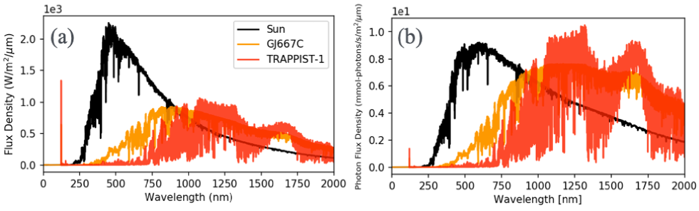
Figure 1: (a) Incident radiation and (b) photon flux density at the top of atmosphere (TOA) of an Earth-like planet around the Sun, GJ667C, and TRAPPIST-1. The spectral data of the Sun, GJ667C, and TRAPPIST-1 were obtained from Meftah et al. (2018), France et al. (2016), and Lincowski et al. (2018), respectively.

2.2 Fluorescence from Photosynthesis

Fluorescence emissions from a planetary surface ${F_{\mathrm{fluor.}}^{{}^{\prime}}}$ are expressed as:

$${F_{\mathrm{fluor.}}^{{}^{\prime}}}(\lambda)=sc_{v}\pi{F_{\mathrm{fluor.}}^{\mathrm{std}}}\times f(\lambda),$$ (3)

where $c_{v}$ is the surface coverage of vegetation (see Section 2.3), $s$ is the scaling factor from the standard observed fluorescence emission reflecting the photosynthetic activity, and ${F_{\mathrm{fluor.}}^{\mathrm{std}}}$ is the standard fluorescence intensity from vegetation based on field measurements. The spectral shape of fluorescence emissions from a photosynthetic organism at wavelength $\lambda$ is defined by $f(\lambda)$. In this study, $F_{\mathrm{fluor.}}^{\mathrm{std}}=1.0$ (W m^-2 $\mu\mathrm{m}^{-1}$ sr^-1) (Du et al., 2019; Yao et al., 2021) and $s=0,1,5,\,\mathrm{and}\,10$. The net fluorescence intensity ${F_{\mathrm{fluor.}}}$ is calculated by considering acquired photons at the habitat using ${F_{\mathrm{fluor.}}^{{}^{\prime}}}$ in Equation (3) as:

$${F_{\mathrm{fluor.}}}(\lambda)=\frac{\chi}{\chi_{0}}{F_{\mathrm{fluor.}}^{{}^{\prime}}}(\lambda),$$ (4)

$$\chi\equiv\int n(\lambda)\sigma(\lambda)d\lambda,$$ (5)

$$\chi_{0}\equiv\int n_{\mathrm{sun,ref.}}(\lambda)\sigma_{\mathrm{chls}}(\lambda)d\lambda,$$ (6)

where $\chi$ is the light absorption efficiency, $n(\lambda)$ is the photon flux density at the planetary surface, and $\sigma(\lambda)$ is the absorption coefficient of a photosynthetic pigment. $\chi_{0}$ represents the standard absorption efficiency on Earth. The subscript chls on $\sigma(\lambda)$ represents chlorophylls (see Chl:abs in Figure 2). $n_{\mathrm{sun,ref.}}(\lambda)$ is the photon flux density on the surface of the Earth from the reference solar spectral irradiance at an air mass of 1.5 (National Renewable Energy Laboratory), which corresponds to a typical irradiance for Earth vegetation.

We considered an incident flux from a star under two sky conditions, a clear sky and 60% cloud cover, to estimate the reflectance at the TOA and $\chi$ on the ground, in accordance with the setup for the simulation. We assumed the clear sky condition, if not specified, and the cloud condition appeared only in Section 4.3.1 (Figure 12). In the cloudy condition, 60% of the radiation is reflected in three kinds of clouds, and 40% of the radiation reaches the ground. For the clouds, we assumed that 40% are low water clouds, 40% are high water clouds, and 20% are high ice clouds (Gao & Kaufman, 2003) at 1, 6, and 12 km altitude, respectively. To model Earth-like conditions, the effect of Rayleigh scattering in a planetary atmosphere was also considered in the cloudy condition using a previously described empirical approach by Bucholtz (1995) (see Appendix A for more details).

Equation (4) indicates that ${F_{\mathrm{fluor.}}^{{}^{\prime}}}$ is linearly scaled to the number of incoming photons that are absorbed by chlorophylls at the planetary surface. In other words, chlorophylls can emit strong fluorescence if the spectral shapes of $n(\lambda)$ and $\sigma(\lambda)$ match well. Note that $n(\lambda)$ is exactly the same as $F^{\downarrow}_{\mathrm{surface}}(\lambda)$, and its unit is shown in Figure 1(b) ($F^{\downarrow}_{\mathrm{TOA}}$ in the figure). This treatment in Equations (3) and (4) can be applied to the relationship between the incoming photons and the photons emitted as fluorescence on an Earth-like planet around various stars other than the Sun.

Figure 2 shows the normalized spectra of fluorescence $f(\lambda)$ and absorption coefficient $\sigma(\lambda)$ for Chls and BChls. The peak wavelength of $f(\lambda)$ is red-shifted from that of $\sigma(\lambda)$, which is called the Stokes shift (Lakowicz, 2006). There are two absorption bands in the $\sigma(\lambda)$ of chlorophylls: the B band (known as the Soret band) in the short-wavelength region and the Q band in the long-wavelength region. The primary fluorescence emission is derived from the Q absorption band. In this study, we modeled $f(\lambda)$ for Chls as the superposition of two Gaussian distributions (Frankenberg et al., 2012; Guanter et al., 2010) with means of 680 nm (PSII) and 740 nm (PSI and PSII). $\sigma(\lambda)$ for Chl uses the model vegetation with chlorophylls ($\sigma_{\mathrm{chls}}(\lambda)$) (Feret et al., 2008). We obtained $f(\lambda)$ and $\sigma(\lambda)$ for BChls from the spectral data for the LH1–RC complex, the supramolecular complex of the light-harvesting core antenna (LH1), and the RC in a bacteriochlorophyll $b$ containing purple photosynthetic bacteria (see Figure 3 in Magdaong et al., 2016)). Note that we used only $\sigma(\lambda)$ in the Q band for calculating $\chi$ and $\chi_{0}$ because free Chls and BChl–protein complexes in each solution affect each spectrum in the B band to different degrees.

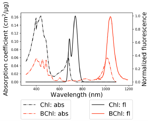
Figure 2: Fluorescence ($f(\lambda)$: solid curves) and photoabsorption ($\sigma(\lambda)$: dashed curves) spectra for chlorophylls (Chl: black) and bacteriochlorophylls (BChl: red). The absorption coefficient of chlorophylls in units of cm² $\mu$g^-1 was obtained from Feret et al. (2008). The fluorescence spectrum is expressed by the Gaussian functions given in Frankenberg et al. (2012) and Guanter et al. (2010). For bacteriochlorophylls, $f(\lambda)$ and $\sigma(\lambda)$ adopt those of the LH1–RC complex of a bacteriochlorophyll $b$ containing purple photosynthetic bacteria (Magdaong et al., 2016). The nondimensional absorption spectrum for BChl is normalized at the peak value in the longest absorption band, the Q band, of the Chl. Two fluorescence spectra are normalized at their peak values.

2.3 Surface Vegetation

To determine the detectability of vegetation fluorescence, we use two leaf models for our experiments: one which assumes the reflectance spectrum and fluorescence of standard chlorophyll and another that uses a scaled version of the spectrum of bacteriochlorophyll. The reflectance of a planet is expressed as $R(\lambda)=\sum_{i}c_{i}r_{i}(\lambda)$, where $i$ denotes the surface type, $c_{i}$ is the fraction of the surface coverage of type $i$, and $r_{i}$ the reflectance of type $i$. We obtained the reflection spectra for various surface types including vegetation, ocean, and coast from the USGS Digital Spectral Library and the ASTER Spectral Library (Baldridge et al., 2009). The detailed compositions used in this paper are summarized in Table 1. The reflectance of the surface vegetation $r_{v}$ is estimated from radiation transfer calculations for a modeled leaf (Jacquemoud & Baret, 1990; Feret et al., 2008), using $\sigma(\lambda)$ over all the wavelengths shown in Figure 2. Figure 3 shows the reflectance of a Chl-based leaf (“standard”) and a BChl-based leaf (“hypothetical”). In the latter case, we assumed the vegetation on a different planet has a photosynthetic pigment whose optical property is the same as BChl exhibiting the VRE in the longer wavelength region as shown in Figure 3. As the input to the radiative transfer calculations, we used the absorption spectra of Chl (Feret et al., 2008) and BChl (Magdaong et al., 2016). The unitless absorption spectrum for BChl is normalized at the peak in that for Chl, unlike the calculations of $\chi$ and $\chi_{0}$ in Section 2.2. As shown in Figure 3, both Chl- and BChl-based leaves show a large reflectance (i.e., the VRE) in the wavelength ranges around 700–750 and 1000–1100 nm. The green bump around 500 nm is observed in the reflectance for Chl, and larger and broader bumps are observed from $\sim$500 to 950 nm for BChls by the larger difference in the wavelength between the B and Q bands than observed for Chl. Like many kinds of photosynthetic organisms, the organisms with BChl could have acquired accessory pigments such as carotenoids (Cars) that absorb photons with wavelengths between the B and Q bands of Chl (Cogdell, 1978). The effective light absorption by accessory pigments can suppress the increase in reflectance. With or without accessory pigments, the bump for BChl does not affect fluorescence emissions in the wavelength (see Figures 7, 8, and  10). The low reflectance from $\sim$500 to 700 nm (1000 nm), due to the light absorption by Chls (BChls), affects the reflectance of the planet. The degree of reduction in the overall planetary reflectance varies depending on the surface coverage by vegetation.

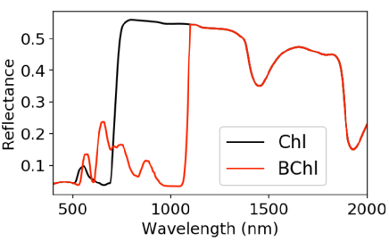
Figure 3: The reflectance of vegetation estimated from radiation transfer calculations for two leaf models: Chl (“standard”) and BChl (“hypothetical”)  (Jacquemoud & Baret, 1990; Feret et al., 2008). The light absorption spectrum for Chls and BChls uses $\sigma(\lambda)$ in Figure 2.

3 Results

We considered three fluorescence cases on an Earth-like planet at different stages of atmospheric evolution around the Sun, GJ667 C, and TRAPPIST-1 for different surface biosignatures: Earth-like (Chl) vegetation, hypothetical BChl-based vegetation, and biological fluorescence without any surface vegetation. Our models for the surface compositions, vegetation, fluorescence types, and atmospheric compositions, i.e., transmittance, are summarized in Table 1. Mod-earth corresponds to the surface condition for the Modern Earth, leading to a lesser contribution of fluorescence emissions than in the other two cases. The veg-only models are considered optimistic conditions for fluorescence emissions where vegetation covers the whole planetary surface. The veg-land models, with 70 % ocean, 2% coast, and 28% land covered with the vegetation, lie between the mod-earth and veg-only models. As mentioned in Section 2, we considered two leaf models for land vegetation: Chl-based vegetation and BChl-based vegetation. For the atmospheric compositions of an Earth-like planet, we adopted the Modern Earth model at 0.0 Ga (oxygen-rich atmosphere), the Paleoproterozoic Earth model at 2.0 Ga (oxygen-poor atmosphere), and the Archean Earth model at 3.9 Ga (anoxic atmosphere) (see Table 1 in Rugheimer & Kaltenegger, 2018). As an extreme case, we assumed the presence of photosynthetic bacteria with BChl spread over the land and ocean on an Archean-Earth-like planet with no surface vegetation. We assumed a clear sky for all atmospheric conditions in Section 3.

Model name	Surface compositions	Surface vegetation	Fluorescence type	$T(\lambda)$	$c_{v}$
veg-only 0C		Chl surf.	Chl fluor.	0.0 Ga
veg-only 2C	100% vegetation			2.0 Ga	1.00
veg-only 0B		BChl surf.	BChl fluor.	0.0 Ga
veg-only 2B				2.0 Ga
veg-land 0C		Chl surf.	Chl fluor.	0.0 Ga
veg-land 2C	70% ocean, 2% coast			2.0 Ga	0.28
veg-land 0B	and 28% vegetation	BChl surf.	BChl fluor.	0.0 Ga
veg-land 2B				2.0 Ga
mod-earth 0C		Chl surf.	Chl fluor.	0.0 Ga
mod-earth 2C	70% ocean, 2% coast			2.0 Ga	0.168
mod-earth 0B	and 28 % mixed land	BChl surf.	BChl fluor.	0.0 Ga
mod-earth 2B	(incl. 16.8% vegetation)			2.0 Ga
anoxic B	70% ocean, 2% coast and	-	BChl fluor.	3.9 Ga	0.72
	28% mixed land at 3.9 Ga

Table 1: Surface composition, vegetation, its fluorescence types, and atmospheric transmittance ($T(\lambda)$) for all the cases in this paper. Mixed land is composed of 60% vegetation (16.8% in total), 15% snow, 9% granite, 9% basalt, and 7% sand (Baldridge et al., 2009); mixed land at 3.9 Ga means the land model of the Archean Earth at 3.9 Ga, which is composed of 35% basalt, 40% granite, 15% snow, and 10% sand. Chl surf. and BChl surf. correspond to reflection spectra of Chl and BChl in Figure 3, respectively. The spectral shapes of fluorescence emissions $f(\lambda)$ for Chl fluor. and BChl fluor. correspond to the fluorescence spectra of Chl and BChl in Figure 2, respectively; their intensities $F_{\mathrm{flour.}}$ are scaled in Equations (3) and (4). $c_{v}$ is given by the relationship between the surface coverage of vegetation and the fluorescence emission. $s$={0, 1.0, 5.0, 10.0}. We obtained $T(\lambda)$ at 0.0, 2.0, and 3.9 Ga from Rugheimer & Kaltenegger (2018).

3.1 Case-1: Planets with Earth-Like Vegetation

In case-1, Earth-like vegetation (Chl) emits fluorescence on the surface of an Earth-like planet. The fluorescence emissions from chlorophyll are visible at the wavelengths from 650 to 800 nm, as shown in Figure 2. To determine the contribution of fluorescence from planets, the reflectance is defined as $F^{\uparrow}_{\mathrm{TOA}}(\lambda)$/$F^{\downarrow}_{\mathrm{TOA}}(\lambda)$ and calculated. Figures 4 and 5 show the reflectance of an Earth-like planet with the Modern Earth’s atmosphere (0.0 Ga) and an oxygen-poor atmosphere (2.0 Ga), respectively. The O₂, O₃, CH₄, and H₂O absorption features in the atmosphere are imprinted in the reflectivity in the visible–NIR wavelengths from 600–800 nm. The oxygen-poor-atmosphere models show less conspicuous patterns in the reflectance profile in the 700 to 750 nm wavelength region. The reflectivity between 600 and 700 nm is nearly constant but increases with decreasing surface coverage of vegetation. The VRE is observed as the steep rise in the reflectance from 700 to 750 nm (also see Figure 3), whereas the reflectance excess due to fluorescence is quite small, even in optimistic conditions (veg-only models). Note that the red curve with $1F_{\mathrm{fluor.}}$ around the Sun in the mod-earth model (Figure 4), corresponding to the modern earth fluorescence, is hardly seen. Around TRAPPIST-1, however, sharp increase in the reflectance around 770 nm is due to the strong absorption of potassium in the stellar atmosphere. As a result, we observed similar features in the light reflected from an Earth-like planet with different atmospheric compositions around TRAPPIST-1 (see Section 4.3.2 for further discussion).

Figure 6 shows the reflectance excess due to fluorescence emissions on an Earth-like planet with the Modern Earth’s atmosphere. Atmospheric absorptions, such as H₂O, O₂, and O₃, weaken the Gaussian features in the fluorescence emissions from an Earth-like planet around the Sun. The fluorescence from chlorophylls around 740 nm is less pronounced for a planet around M dwarfs than one around the Sun because of weaker radiation flux in the wavelength region of 700–750 nm (see Figure 1). In addition, a sudden increase in reflectance due to the VRE obscures the fluorescence emission around 740 nm (see Figures 4 and 5). As a result, the Chl fluorescence around 680 nm emitted from PSII on an Earth-like planet would be the most promising feature for detection (see Figure 2). Note that nonphotochemical quenching processes can decrease the fluorescence intensity around 680 nm, and the fluorescence emission is further reduced by the reabsorption of photons within the canopy (Porcar-Castell et al., 2021).

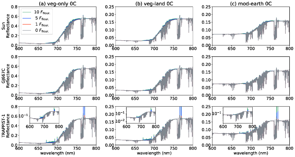
Figure 4: Reflectance of an Earth-like planet with the Modern Earth’s atmosphere (0.0Ga) around the Sun, GJ667C, and TRAPPIST-1. The three colors represent the reflected light from a planet with $F_{\mathrm{fluor.}}$ ($s=1$: red), $5F_{\mathrm{fluor.}}$ ($s=5$: blue), and $10F_{\mathrm{fluor.}}$ ($s=10$: green), where $F_{\mathrm{fluor.}}$ is the fluorescence emission from chlorophylls observed on the Earth. No-fluorescence emission models are also indicated by gray lines. We assumed Earth-like vegetation (chlorophylls) covers the planetary surface (see Table 1 for model details). The reflectance is defined here as $F^{\uparrow}_{\mathrm{TOA}}(\lambda)$/$F^{\downarrow}_{\mathrm{TOA}}(\lambda)$, where $F^{\uparrow}_{\mathrm{TOA}}(\lambda)$ is the light reflected from the ground at the top of atmosphere (TOA), and $F^{\downarrow}_{\mathrm{TOA}}(\lambda)$ is the flux at TOA induced by stars. For each case around TRAPPIST-1, the reflectance with a logarithmic scale is also shown as the inset plot.

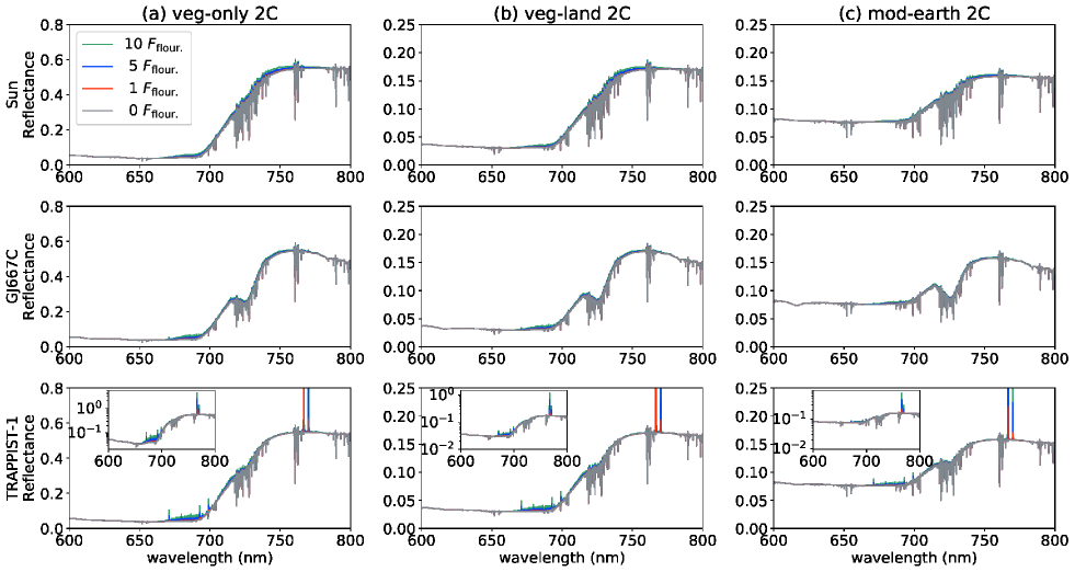
Figure 5: The same as Figure 4, but for an Earth-like planet with an oxygen-poor atmosphere (2.0 Ga).

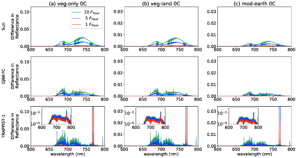
Figure 6: Reflectance excess due to chlorophyll fluorescence emissions on an Earth-like planet with the Modern Earth’s atmosphere.

3.2 Case-2: Planets with Bacteriochlorophylls-Based Vegetation

In case-2, BChl-based vegetation, as the major photosynthetic pigment, covers the surface of a planet. The BChls are assumed to emit the same degree of fluorescence intensity as the Earth’s vegetation. As shown in Figure 2, fluorescence from BChls occurs in the wavelength range from 1000 to 1100 nm. In contrast to case-1, fluorescence emissions with 5 and $10F_{\mathrm{fluor.}}$ show strong features around 1050 nm in almost all conditions in Figures 7 and 8. Identifying the fluorescence on the Earth’s vegetation level ($\lesssim F_{\mathrm{fluor.}}$) is still challenging even in the optimistic case, that is, (a) veg-only 0B. The reflectivity between 1000 and 1050 nm becomes slightly higher for mod-earth models with less surface vegetation coverage. As shown in Figure 9, the BChl organisms efficiently absorb photons and emit fluorescence with less absorption and scattering in the planetary atmosphere. The fluorescence emissions from BChls that we assumed are invulnerable to blending with the steep increase in the reflectance by the VRE. As a result, we found a more significant fluorescence contribution to the reflected light in case-2.

Atmospheric properties, such as chemical compositions and cloud coverage, change the fluorescence profile. The water absorption is weak for wavelengths from 1000 to 1100 nm. If the major absorption bands of a photosynthetic pigment lie in wavelengths longer or shorter than 1000–1100 nm, the presence of water vapor in the atmosphere complicates the detection of fluorescence emissions. A strong absorption due to CH₄ in an oxygen-poor atmosphere also hides fluorescence near 1000 nm (see the GJ667C models in Figure 8). The BChl organisms bearing BChl $b$ and their Stokes shift are ideal for detecting fluorescence in wavelengths longer than the characteristic wavelength of fluorescence from Chls. Thus, fluorescence in the wavelength range of 1000 -1100 nm could be a suitable biosignature for photosynthetic organisms, such as bacteriochlorophylls, on planetary surfaces unless they coexist with strong absorbers near 1000 nm.

The VRE with a sharp rise in the reflectance is observed in the wavelength range from 1050 to 1100 nm in case-2, as shown in Figure 3. Reflectance excess due to BChl fluorescence is 0.01–0.05 for the Modern Earth atmosphere models (see Figure 9), whereas that due to the VRE is 0.4–0.5 (0.1–0.15) for veg-only models (veg-land and mod-earth models). Bacteriochrolophylls’ fluorescence causes a slight increase in reflectance around 1000 -1100 nm compared to the VRE. Such nonprominent fluorescence emission with a Gaussian shape in the wavelength different from the VRE feature can be extracted from the reflectance profile using data processing such as principal component analysis (PCA). Photosynthetic organisms different from those around the Sun are expected to exhibit VRE and fluorescence features in different wavelengths. Thus, not only spectral features due to atmospheric molecules but also the simultaneous detection of the VRE and the fluorescence will help identify traces of photosynthesis on an exoplanet. Probably, when we found a possible signal of VRE, the fluorescence would be useful for further validation, because the VRE signal is stronger than the fluorescence one.

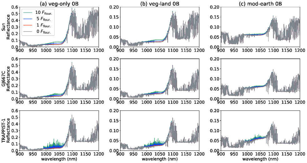
Figure 7: The same as Figure 4 but for the reflectance of a planet covered with bacteriochlorophyll-based vegetation.

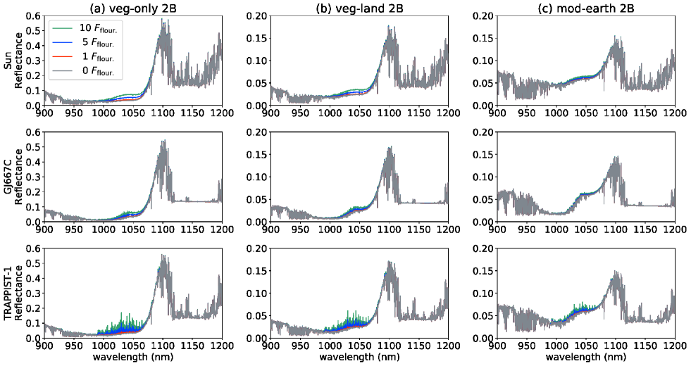
Figure 8: The same as Figure 7, but for a planet with an oxygen-poor atmosphere (2.0 Ga).

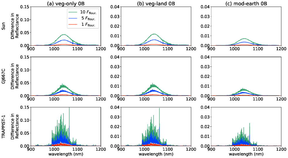
Figure 9: Reflectance excess due to bacteriochlorophyll fluorescence emissions on an Earth-like planet with the Modern Earth’s atmosphere.

3.3 Case-3: Anoxic World (without VRE)

In case-3, an Earth-like planet has the same reduced atmosphere as the Archean Earth at 3.9 Ga. Anoxic bacteria with photosynthetic pigments such as bacteriochlorophylls may spread over the surface of a planet with a CO₂-rich atmosphere. Anoxic bacteria are assumed to live in the ocean and coast (i.e., $c_{v}=0.72)$ and emit only fluorescence whose intensity is comparable to the standard emission from land plants, without the distinct reflectance of a vegetation surface. Fluorescence emissions from anoxic bacteria adopt those from bacteriochlorophylls on the Earth. Figure 10 shows the reflectance of an Archean-Earth-like planet with BChl-based bacteria. In the reflection spectra, a strong water absorption appears around 950 and 1150 nm. The relatively high reflectance across the wavelength range is mainly from the light reflected by the land. We observe fluorescence emissions in the wavelength range between 1000 and 1100 nm owing to the lack of light reflected from BChl-bearing oceanic bacteria, including the VRE feature. Intense absorption in the stellar atmosphere enhances the apparent reflectance of a planet around TRAPPIST-1 (see also Figures 4 and 5, and Section 4.3.2).

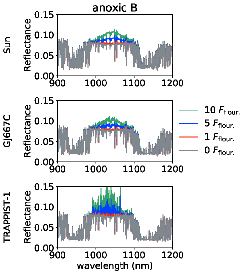
Figure 10: The reflectance of an Earth-like planet with an anoxic atmosphere and no land vegetation (anoxic B).

4 Discussion

This study demonstrated reflectance with photosynthetic fluorescence on an Earth-like planet around the Sun and two M dwarfs. This section reviews the biological processes of photosynthesis and then considers the future detection of biofluorescence on an exoplanet. In Section 4.1, we discuss the possible physiological conditions that enhance the fluorescence emissions on a planet based on our understanding of Chl fluorescence. In Section 4.2, we discuss the possible false positive or negative detection of fluorescence (Section 4.2.1), and the potential usage of the nonlinear photoresponse in fluorescence yield to excitation light intensity to distinguish between biofluorescence and the false positive/negative signals of fluorescence (Section 4.2.2). Finally, in Section 4.3, we show the fluorescence detection with telescopes. We present the detectability of fluorescence from an Earth twin around a Sun-like star u sing the noise model for a LUVOIR-A-like mission (Section 4.3.1), and the remarkable enhancement in the reflectance due to the absorption lines of stars, which could be a promising feature for detection by high-dispersion spectroscopy, especially around ultracool stars (Section 4.3.2).

4.1 Possible Physiological Conditions for Supporting Fluorescence Detection

This study adopted the typical fluorescence spectrum of Chl-containing plants and LH1–RC purified from BChl $b$-bearing purple bacteria. The fluorescence spectrum of the LH1–RC complex suspended in buffer solution was measured under laboratory conditions with a low concentration of LH1–RC in the solution to avoid the reabsorption of fluorescence. Cells having LH1-RC in vivo would result in an $\sim 50$ nm shift in the spectral peak wavelength toward longer wavelengths under dense conditions, because the reabsorption of fluorescence reduces the shorter-wavelength part of fluorescence. A red-shifted fluorescence spectrum should still be observable because it is located within the atmospheric window. For the fluorescence intensity of vascular plants on the ground, we referred to the standard value ($F_{\rm fluor.}$) for the fluorescence model on exoplanets in our simulations. The possible detection of fluorescence emissions on exoplanets would require $\gtrsim 5F_{\rm fluor.}$ with BChl (see Figures 7, 8, and 10). There are four potential factors that increase the fluorescence yield in photosynthetic organisms from the biophysical viewpoint of photosynthetic studies on existing phototrophs on the Earth:

1. Increasing Chl/BChl concentration per land area

   A high concentration of Chls and BChls enhances their fluorescence intensity. In general, the Chl/BChl concentration in a cell increases for capturing as many photons as possible under low light conditions. Fluorescence increases linearly with Chl/BChl concentration when cell density is low. In contrast, the fluorescence intensity reaches a saturation level in highly dense environments due to the reabsorption of fluorescence by cells (Du et al., 2017).

2. Small spectral overlap between absorption and fluorescence

   The large separation between the main absorption band and its fluorescence band increases the fluorescence intensity of concentrated cells. In photosynthetic organisms, the excitation energy is transferred between Chls, and the Chl fluorescence tends to be emitted from long-wavelength Chls (LWC), which has the reddest absorption band in a photosystem because the excess excitation energy is easily trapped at the lowest energy level. A redshift in the peak wavelength of fluorescence and a blueshift in absorption, which can be caused by the modification of the vibronic interactions of pigments between surrounding proteins and solvent, reduce the spectral overlap between fluorescence and absorption. The fluorescence emission from LWCs is red-shifted to over 50 nm from that of bulk Chls in some conditions. Although most plants have a small amount of LWCs in PSII and the Chl fluorescence is absorbed well under high Chl concentrations, far-red absorbable LWC contributing to PSII has been reported in some eukaryote algae (Fujita & Ohki, 2004; Wilhelm & Jakob, 2006; Kotabová et al., 2014; Wolf et al., 2018; Kosugi et al., 2020). These algae show a significant fluorescence emission at far-red-light wavelengths (700–800 nm) at room temperature, and some of them decrease the overlap (Fujita & Ohki, 2004; Kosugi et al., 2020).

3. Low photosynthetic efficiency

   Photon loss in photosynthetic processes reduces the photon yield of fluorescence. Excitation yield in PSII has increased throughout the evolutionary processes of photosystems. For example, the increase in light use efficiency in oxygenic photosynthesis on Earth was achieved by changing the light-harvesting antenna protein from the membrane superficial phycobilisome in cyanobacteria to the light-harvesting Chl binding protein in eukaryotic algae. Furthermore, the subsequent modification of LHCs achieved a higher photosynthetic quantum yield in the evolution process. The maximum excitation yield in PSII of vascular plants is estimated to be $\sim$ 0.9, whereas that of green algae and cyanobacteria is $\sim$ 0.8 and $\sim$ 0.6, respectively (Schuurmans et al., 2015). Suppose phototrophs on an exoplanet are in the early stage of evolution. In that case, the expected fluorescence yield may be high to compensate for the low efficiency of photon yields in primitive photosynthesis.

4. Suppression of heat dissipation

   Photon loss by the heat dissipation in photosynthetic pigments suppresses the photon yield of fluorescence. Heat dissipation occurs in the vibrational relaxation of excited pigment molecules, Chls, or accessory pigments such as carotenoids. Additionally, light-dependent protection mechanisms to dissipate the excess light energy as heat are inherent in all the cyanobacteria, algae, and plants. The efficiency of heat dissipation largely depends on the molecular configuration and the environment of pigments binding to proteins. The energy conversion rate from light to heat in photosystems is crucial in estimating photosynthetic fluorescence on other planets.

Therefore, the fluorescence yield in photosynthetic pigments should fluctuate over time due to photosynthetic activity and heat dissipation.

4.2 Further Identification for Confirming Photosynthetic Fluorescence

4.2.1 Potential false positive/negative of biological fluorescence detection from exoplanets

Photosynthetic pigments on an exoplanet may be different from those on Earth, and the wavelength relevant to fluorescence emission from exovegetation remains to be unknown. A possible fluorescence signal on other planets can be a false positive or negative detection of biological activities. Potential main sources causing false positive/negative could be surface reflectance or fluorescence from minerals on exoplanets. Both Chl and BChl fluorescence in our study can be contaminated by mineral fluorescence, but it is not plausible to expect the fluorescent minerals to cover a fraction of a planetary surface comparable to Earth’s vegetation as far as our knowledge of the Earth’s environment. Recently, solar-induced mineral luminescence (SML) has been extracted from SIF data obtained by remote sensing of the Earth (Köhler et al., 2021). They revealed that about 10$\%$ of non-vegetated areas are weakly luminescent and speculated that luminescence came from some spots covered by carbonate with Mn²⁺ and was comparable to SIF (or Chl fluorescence). However, those areas are negligible on the planetary scale. On the other hand, mineral fluorescence could pollute, to an extent, fluorescence in near-infrared, which includes the BChl fluorescence. For instance, silicate (e.g., pyroxene and olivine) shows a prominent absorption around 1000 nm caused by Fe²⁺ (Bishop et al., 2019; Klima et al., 2011; Sunshine & Pieters, 1998). Its fluorescence could appear in a slightly longer wavelength from the absorption, whose energy corresponds to the Stokes shift, like other near-infrared fluorescent materials (Jackson et al., 2021; Selvaggio et al., 2020). While there are a variety of fluorescent minerals (e.g., fluorite, calcite, corundum), we do not deny the possibility that the unexpectedly strong mineral fluorescence could be observed on exotic planets such as a carbide exoplanet (Allen-Sutter et al., 2020) whose surface could be covered by diamond with lattice defects, e.g., due to nitrogen-vacancy center (Schirhagl et al., 2014). To understand potential fluorescence features from surface components of an exoplanet, e.g., rocks and minerals, characterizing atmospheric features is helpful. Besides, as mentioned so far, the simultaneous detection of vegetation reflectance (VRE) and fluorescence features could help identify photosynthesis.

4.2.2 Nonlinear photoresponse in photosynthesis

Photosynthetic organisms regulate metabolic processes to maximize the use of available photons under light conditions and emit biological fluorescence by converting light energy via photochemical reactions. The nonlinear response of the fluorescence yield to the excitation light intensity would be a clue to finding the presence of photosynthetic organisms. If a planet is in an elliptical orbit, the incident flux received by the planet from its host star varies with time. Fluorescence emissions from nonbiological processes increase with incident light intensity. In contrast, a saturation level of the fluorescence intensity from biological activities, such as photosynthesis, exists because the quantum yields of Chl fluorescence vary according to the light environment and atmospheric CO₂ concentrations. The quantum yields of Chl fluorescence are primarily involved in the reduction states of electron acceptors of photosystems for electron transports and excitation energy quenching by photoprotection mechanisms (see Genty et al., 1989; Krause & Weis, 1991; Baker, 2008). A sudden intense light can induce the reduction in the electron acceptors of PSII, where oxidation of water to generate O₂ occurs as a primary step in photosynthesis. The presence of photoprotection mechanisms also modulates the quantum yields of Chl fluorescence. When dark- or dim-light-adapted leaves are suddenly irradiated with intense light, Chl fluorescence quantum yields rapidly increase by up to five times. Accordingly, the relationship between fluorescence yield and excitation light intensity (i.e., the number of absorbed photons) provides a hint to explore the origin of fluorescence on a planet.

4.3 Detectability of Biological Fluorescence by Future Telescopes

4.3.1 The Earth-Sun System as an Earth Twin in a LUVOIR-A-Like Mission

We investigated the detectability of fluorescence from an Earth twin around a Sun-like star at 10 pc from the Earth, assuming a LUVOIR-A-like space telescope. Figure 11 presents the simulated spectra of a second Earth around a Sun-like star at 10 pc with the biological fluorescence. We applied the noise model used in Robinson et al. (2016) and Kopparapu et al. (2021), which accounts for planet photons, stellar photon noise, and background noise, e.g., zodi, exozodi, read-out, and dark current noises with the throughput assuming the LUVOIR-A telescope. The parameters and the formalism used in this paper are presented in Appendix B. Figures 11(a–c) show the results of the most optimistic model for the fluorescence signal (veg-only 0B) from the Earth-Sun system observed from 10 pc with a 15 m space telescope. The original data are the same as those of the Sun in Figure 7(a). In Figure 11(a), $F_{\rm p}/F_{\rm s}$ observed at the telescope for each wavelength bin is shown as solid lines, with the random noise as the 1$\sigma$ error bars for each bin, in 9000 hours of exposure time, where $F_{\rm p}$ is the reflected light from the planet and $F_{\rm s}$ is the starlight. Figure 11(b) depicts a magnification of the spectrum in Figure 11(a). Some error bars are outside the solid line, but the spectral feature of fluorescence emission is recognizable for each case in the figure. Figure 11(c) shows the SNR with the same observation time as that in Figure 11(a). The difference between 0 and 5 $F_{\rm{fluor.}}$ is larger than 1$\sigma$. To detect the fluorescence with 3$\sigma$ error, $\sim$ 50000 hours of exposure time are required, and with 5$\sigma$, $\sim$ 100000 hours, ten years, are expected (not shown in figures). Thus, fluorescence detection would require years for observation, even by the LUVOIR-A-like space telescope, and it is extremely challenging to observe one target. In less optimistic models, namely, the veg-land 0B model around the Sun in Figure 7(b), the detection of fluorescence signals is even more challenging, as shown in Figure 11(d). As discussed in Section 3.2, the fluorescence in mod-earth 0B is difficult to identify. Moreover, cloud coverage obscures the VRE features as well as atmospheric features on exoplanets (Seager et al., 2005; Tinetti et al., 2006; Kaltenegger et al., 2007). The reflectance in Figure 12 indicates how clouds suppress the fluorescence signal. Even in the most optimistic model, the fluorescence in the reflectance is significantly reduced and can hardly be observed. In the mod-earth model, it is impossible to identify the fluorescence signals. The only possible way to observe surface vegetation with significant cloud coverage, except for atmospheric gases, would be the VRE ($\sim$0.1 in reflectance in the optimistic model). Thus, the existence of water clouds that are expected in Earth-like planets with surface water seems to be critical for fluorescence detection. However, around TRAPPIST-1, as the relevant argument was shown in Session 4.3.2, we found that the Chl fluorescence in the K $\rm{I}$ lines was insensitive to the coverage by Earth clouds, which could be an advantage in the Chl detection over BChl one.

The fluorescence feature would be poorly determined with 900 hours of exposure time with 1$\sigma$ errors, whereas the VRE feature can be identified. Even for a LUVOIR-A-like space telescope, an enormous observational time would be needed to identify the fluorescence in addition to the VRE with more confidence for detecting traces of photosynthesis. We also investigated the detectability of fluorescence by a space telescope with a different diameter. A 6 m space telescope is recommended for future space missions, according to Astro2020 Decadal Survey. With a 6-m diameter, $\sim$ 300,000 hours of observation time are required to identify fluorescence. When we adopt a 30 m space telescope with 1$\sigma$ errors, the required exposure time is reduced to $\sim$ 800 hours. Furthermore, one of the background noises, i.e., the readout noise, can be suppressed with data processing because of increasing reads in an exposure as implemented for H2RG infrared detectors (e.g., Brandt et al., 2017; Kuzuhara et al., 2018). When the readout noise is assumed to be zero all over the wavelengths, the required observation times are reduced to $\sim$ 250,000, $\sim$ 7,000 and $\sim$ 500 hours with the 6-, 15-, and 30-m diameters.

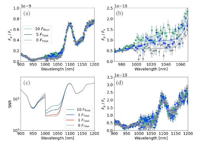
Figure 11: Simulated spectrum with the biological fluorescence on a second Earth around a Sun-like star at 10 pc from the Earth, assuming a LUVOIR-A-like space telescope. (a–c) The results from the veg-only 0B model and (d) $F_{\rm p}/F_{\rm s}$ with the veg-land 0B model. (a) $F_{\rm p}/F_{\rm s}$ with 9000 hours of observation time. The solid line shows $F_{\rm p}/F_{\rm s}$ and the error bar indicates the noise at each wavelength. (b) A magnification of $F_{\rm p}/F_{\rm s}$ in (a). (c) The SNR in (a).

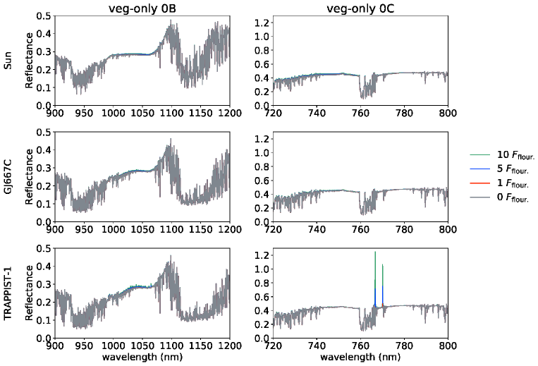
Figure 12: The effect of cloud on the reflectance with veg-only 0B and 0C models. The models are the same as the veg-only 0B in Figure 7 and the veg-only 0C in Figure 4 but with cloud coverage.

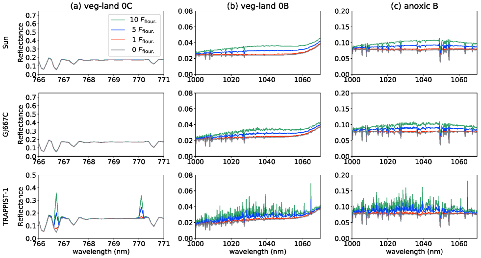
Figure 13: The apparent enhancement of fluorescence in reflectance due to stellar absorption around the three template stars: (a) veg-only 0C model (Figure 4), (b) veg-only 0B model (Figure 7), and (c) anoxic B model (Figure 10).

4.3.2 Apparent Enhancement in Fluorescence around Ultracool Stars and Possible Detection with High-Dispersion Spectroscopy

Figure 13 shows the contribution of fluorescence around three host stars. Around TRAPPIST-1 the apparent enhancement in reflectance induced by fluorescence is significant compared to around the other two stars because TRAPPIST-1 has strong absorption features spanning the wavelengths of the fluorescence. Within the TRAPPIST-1 stellar absorption features, reflected light from the planet is reduced, allowing the fluorescence emission to become a much larger fraction of the outgoing flux (reflected + fluorescence) at these wavelengths. This is analogous to the methodology of SIF detection with remote sensing observations and the retrieval processes by determining how much the fluorescence influences the Fraunhofer lines (Maier et al., 2004). These spectroscopic features may be widely used for fluorescence detection around ultracool stars.

Figure 13(a) shows that the reflectance is highly enhanced due to the absorption lines of K $\rm{I}$ in the stellar spectrum of TRAPPIST-1, which is not affected by water clouds (Figure 12). The degree of enhancement for each line depends on the atmospheric compositions of an Earth-like planet. Figure 13(b,c) presents a spiky feature due to absorption of FeH and VO, as commonly observed around ultracool stars. Therefore, observing the possible fluorescence signal with high spectral resolution using extremely large ground telescopes would be worthwhile.

5 Conclusions

In this paper, we explored fluorescence from photosynthesis as a biosignature on an exoplanet for future observations in great detail and identified the situations in which the signal could be enhanced, and the regions of the spectrum where fluorescence from chlorophylls and bacteriochlorophylls could be most detectable for Earth-like planets around different stars. We also described how we could enhance the possibility to more definitively detect the action of photosynthesis. For direct imaging observations, however, we found that the detection of fluorescence emissions would be extremely challenging to observe and especially not feasible for the planned 6m space telescope. More details are provided as follows.

We considered fluorescence emissions from Chl- and BChl-based vegetation in a clear-sky condition on an Earth-like planet around the Sun and two M dwarfs (GJ667 C and TRAPPIST-1). Chl- and BChl-based leaves show a VRE in wavelengths around 700–750 and 1000–1100 nm. The fluorescence emissions from Chls and BChls occur at wavelengths from 650 to 800 nm and 1000 to 1100 nm, corresponding to the longest Q absorption band of each pigment. The two peaks of Chl fluorescence at 680 and 740 nm arise from the PSII and PSI, respectively. Thus, atmospheric absorption bands, such as H₂O, CH₄, O₂, and O₃, and the VRE could be overlapped with the fluorescence emissions from Chls and BChls. Chl fluorescence emission from PSI is blended with the steep VRE feature. Fluorescence emitted from PSII on an Earth-like planet is the most promising feature for observation, but it may also be reduced by nonphotochemical quenching processes and reabsorption of photons by surrounding Chls. Conversely, the fluorescence emitted from BChls is not suppressed by the sharp increase in the reflectance due to the VRE and atmospheric absorption by, for example, water vapor, except for CH₄ absorption around 1000 nm. Therefore, the BChl fluorescence in the wavelength range of 1000–1100 nm, rather than Chl fluorescence, may be a more promising biosignature from photosynthetic organisms on a planetary surface. In both cases of Chl- and BChl-based vegetation, the simultaneous detection of the VRE and fluorescence is significant for identifying photosynthetic activity on an exoplanet, because we do not know exactly what kind of vegetation exists in the planet in principal and we need more information for further validation to identify the trace of photosynthesis. If BChl-bearing photosynthetic bacteria inhabit water without any leaf or tree structures, the fluorescence spectrum is the only surface reflectance feature that can be used to access such underwater photosynthetic organisms, although the fluorescence signal would be reduced according to the opacity of overlying liquid water.

Based on our understanding of photosynthesis, the intensity of fluorescence is lower in photosynthetic bacteria compared to land plants. Here, we presented four factors that enhance the fluorescence emission for possible detection of biological fluorescence on an exoplanet: (1) increase in Chl/BChl concentration per land area, (2) small overlap of absorption and fluorescence spectrum, (3) low photosynthetic efficiency, and (4) suppression of heat dissipation. This study assumed a linear photoresponse of fluorescence to excitation light intensity. If a planet is on a large elliptical orbit and the telescope has sufficient sensitivity to temporally resolve changes in fluorescence as a function of time, the nonlinear photoresponse from the biological fluorescence can be identified. Assuming a LUVOIR-A-like mission, an enormous duration (around 9000 hours) would be required to detect the BChl fluorescence emission, whose fluorescence yield is 5–10 times larger than that of vegetation on Earth in the optimistic cases for an Earth-Sun twin at a distance of 10 pc from the Earth. In addition, the cloud coverage significantly affects the detection of fluorescence as well as other spectral features because the cloud more strongly obscures fluorescence emissions than the VRE feature. Interestingly, the fluorescence in the reflectance was found to be remarkably enhanced in all three cases around TRAPPIST-1 because of its strong absorption in the stellar atmosphere, like the SIF detection by remote sensing using Fraunhofer lines. The reflectance excess due to K $\rm{I}$ absorption and VO/FeH absorption can be a promising feature for characterizing the fluorescence around ultracool stars in Chl and BChl cases. Note that Chl fluorescence in K $\rm{I}$ lines was still prominent with water clouds.

Thus, one of the most important future works would be the mock observation assuming a 30 m class ground-based telescope to investigate how the apparent enhancement in reflectance due to stellar absorption could help the fluorescence detection around ultracool stars. In addition, to better support the future detection of fluorescence emissions on an exoplanet, further studies are required from various perspectives. For example, planetary spectra for a wide range of atmospheric and surface conditions consistent with biological fluorescence emission should be estimated and tested using radiation transfer calculations because our studies considered still-limited conditions. Moreover, we need to conduct simulations on how the fluorescence is observed on an exoplanet when a global SIF map data from remote sensing of the Earth are applied. Also, experimental validation of prominent NIR fluorescence emissions is needed in some species of photosynthetic organisms and conditions.

Appendix A Empirical Rayleigh Scattering

The effect of Rayleigh scattering is implemented empirically as follows (Bucholtz, 1995):

$$\tau_{\mathrm{R}}(\lambda) = \beta_{\mathrm{s}}(\lambda)\frac{T_{\mathrm{s}}}{P_{\mathrm{s}}}\int_{0}^{z^{\prime}}\frac{P(z)}{T(z)}dz,$$ (A1)

where $\tau_{\mathrm{R}}$ is the Rayleigh optical depth at altitude $z^{\prime}$; $T(z)$ and $P(z)$ are the temperature and pressure at $z$, respectively. We adopted the $T-P$ profile in the U.S. standard atmosphere 1976 from 0 to 60 km to compute the Rayleigh scattering cross-section in the atmosphere of an Earth-like planet. The actual $T-P$ profile in the atmosphere of an Earth-like planet around a star other than the Sun is quite different from that in the Earth’s atmosphere. Rayleigh scattering, however, has a negligible effect on the transmittance at wavelengths from 600 to 1100 nm ($\approx$ 6 $\%$ in transmittance at 600 nm, reducing with increasing wavelength, and then $<$ 1 $\%$ at 1100 nm for an Earth-like planet around the Sun, for instance), which is closely related to the fluorescence from Chls and BChls. $T_{\mathrm{s}}$ and $P_{\mathrm{s}}$ are the temperature and pressure at standard conditions on Earth, respectively ($T_{\mathrm{s}}$ = 288.15 K and $P_{\mathrm{s}}$ = 1013.25 mbars). The total Rayleigh volume-scattering coefficient $\beta_{s}$ is expressed as:

$$\beta_{s}(\lambda)=A\lambda^{-B-C\lambda-D/\lambda},$$ (A2)

where the coefficients $A,B,C$, and $D$ are empirically determined (see Table 3 in Bucholtz (1995)).

Parameter	Description	Adopted Value
$D$	Mirror Diameter	6, 15, 30 m
$C$	Raw Contrast	$10^{-10}$
$R$	Instrumental spectral resolution	70
$T_{\mathrm{Tele}}$	Accounts for light lost due to contamination	0.95
	and inefficiencies in the main collecting area
$T_{\mathrm{read}}$	Read-out efficiency	0.75
$T_{\mathrm{QE}}$	Raw quantum efficiency	0.9
$f_{\mathrm{pa}}$	Fraction of planetary light that falls within photometric aperture	1
$X$	Width of photometric aperture as multiple of $\lambda/D$	0.61 arcsec
$N_{\mathrm{ez}}$	Number of Exozodis	4.5
$D_{e-}$	Dark current (UVIS/NIR)	3E-5/2E-3 $e^{-}/s$
$R_{e-}$	Read noise per pixel (UVIS/NIR)	0/2.5 $e^{-}$
$\theta_{\mathrm{IWA}}$	Inner working angle of the coronagraph as multiple of $\lambda/D$	3
$\lambda_{0}$	Diffraction limit at the wavelength	500 nm

Table 2: Parameters for simulations based on a LUVOIR-A-like mission.

Appendix B LUVOIR Noise Model

We implemented a noise model assuming a LUVOIR-A-like mission. The formalism and the parameters are based on Robinson et al. (2016), but, as shown in Table 2, we updated some parameters (with several treatments) following Kopparapu et al. (2021) for our simulations with the LUVOIR-A telescope.

The total noise in the observation $C_{\mathrm{total}}$ is calculated by:

$$C_{\mathrm{total}} = C_{\mathrm{p}}+C_{\mathrm{s}}+C_{\mathrm{b}},$$ (B1)

where $C_{\mathrm{p}}$ is the number of planet photons, $C_{\mathrm{s}}$ is the stellar photon noise (leakage through the coronagraph), and $C_{\mathrm{b}}$ is the background noise, which is the sum of zodi $C_{\mathrm{z}}$, exozodi $C_{\mathrm{ez}}$, dark current $C_{\mathrm{D}}$, and readout noise $C_{\mathrm{R}}$. The internal thermal noise is ignored because the thermal contribution is negligible in our wavelengths of interest. Note that the noise in Equation B1 corresponds to variance rather than the standard deviation. The noise count is expressed as:

$$C_{\mathrm{noise}} = \sqrt{C_{\mathrm{p}}+C_{\mathrm{s}}+2C_{\mathrm{b}}}$$ (B2)

where the double $C_{\mathrm{b}}$ accounts for the on-off observation with and without the planet. The on-off observation corresponds to the subtraction of point spread functions of a central star. $\mathrm{S}/\mathrm{N}$ for each wavelength $\lambda$ is defined by:

$$S/N = \frac{C_{\mathrm{p}}}{C_{\mathrm{noise}}}.$$ (B3)

The $F_{\mathrm{p}}$ and $F_{\mathrm{s}}$ are now defined to be the reflected light from a planet and the stellar flux acquired by the telescope at a wavelength (bin) $\lambda$. When observing $F_{\mathrm{p}}/F_{\mathrm{s}}$, the $1\sigma$ error at $\lambda$ is given as:

$$\sigma(\lambda) = \frac{F_{\mathrm{p}}}{F_{\mathrm{s}}}\frac{1}{\mathrm{S}/\mathrm{N}}.$$ (B4)

The end-to-end throughput for planetary fluxes is calculated as:

$$T_{\mathrm{total}} = T_{\mathrm{Tele}}T_{\mathrm{cor}}T_{\mathrm{opt}}T_{\mathrm{read}}T_{\mathrm{QE}},$$ (B5)

where $T_{\mathrm{Tele}}$ is an account for light lost due to contamination and inefficiencies in the main collecting area, $T_{\mathrm{read}}$ is the read-out efficiency, and $T_{\mathrm{QE}}$ is the raw quantum efficiency for the detector. The coronagraphic $T_{\mathrm{cor}}$ and the optical $T_{\mathrm{opt}}$ throughputs are the same as in Figure 9 in Kopparapu et al. (2021).

We updated the formalism on noise from zodis, exozodis, and readout as follows; In Robinson et al. (2016), the spectral shape of zodis (exozodis) was assumed to be equal to that of the Sun (the host star). Instead, we explicitly adopt the normalized reflectance on solar zodis, $\tilde{R}_{\odot,\lambda}$, in the model to better account for the zodical light in a exoplanetary system. We calculate $\tilde{R}_{\odot,\lambda}$ by tracing the spectral data from observations of the zodical light (see Figure 8 in Kawara et al. (2017) and Figure 10 in Tsumura et al. (2010)) with the normalization in the $V$ band. Using $\tilde{R}_{\odot,\lambda}$, the noise from zodis is expressed as:

$$C_{\mathrm{z}} = \frac{\pi\lambda^{2}D^{2}}{4hcR}\frac{F_{\odot,\lambda}(1\mathrm{au})}{F_{\odot,V}(1\mathrm{au})}\tilde{R}_{\odot,\lambda}F_{0,V}10^{-M_{\mathrm{z},V}/2.5}T_{\mathrm{total}}\Omega\Delta t_{\mathrm{exp}},$$ (B6)

where $F_{\odot,\lambda}$ is the solar flux density at $\lambda$, $F_{\odot,V}$ is the solar flux density in the $V$ band, $h$ is the Planck constant, $c$ is the speed of light, $M_{\mathrm{z},V}$ = 23 mag arcsec^-2 is the $V$-band zodical-light surface brightness, and $\Delta t_{\mathrm{exp}}$ is the exposure time. The circular photometry aperture size is expressed as $\Omega=\pi(X\lambda/D)^{2}$. Assuming the exozodis’s reflectance to be the same as $\tilde{R}_{\odot,\lambda}$, the noise from exozodis is written as:

$$C_{\mathrm{ez}} = \frac{\pi\lambda^{2}D^{2}}{4hcR}\left(\frac{1\mathrm{au}}{r}\right)^{2}\frac{F_{\mathrm{s},\lambda}(1\mathrm{au})}{F_{\mathrm{s},V}(1\mathrm{au})}\frac{F_{\mathrm{s},V}(1\mathrm{au})}{F_{\odot,V}(1\mathrm{au})}\tilde{R}_{\odot,\lambda}F_{0,V}N_{\mathrm{ez}}10^{-M_{\mathrm{ez},V}/2.5}T_{\mathrm{total}}\Omega\Delta t_{\mathrm{exp}},$$ (B7)

where $F_{\mathrm{s},\lambda}$ is the stellar flux density at $\lambda$, $F_{\mathrm{s},V}$ is the stellar flux density in the $V$ band, and $r$ is the distance between the planet and the parent star. $M_{\mathrm{ez},V}$ = 22 mag arcsec^-2 is the $V$-band exozodical light surface brightness. Even if the original treatment of exozodical light is adopted, our results do not significantly vary. We calculate the read-out noise ($C_{\mathrm{R}}$) to be $C_{\mathrm{R}}=N_{\mathrm{pix}}N_{\mathrm{read}}R_{\mathrm{e^{-}}}^{2}$ instead of $C_{\mathrm{R}}=N_{\mathrm{pix}}N_{\mathrm{read}}R_{\mathrm{e^{-}}}$ in Robinson et al. (2016) to more realistically incorporate the noise propagation, where $N_{\mathrm{pix}}$ is the number of contribution pixels, $N_{\mathrm{read}}$ is the number of reads at each observation, and $R_{\mathrm{e^{-}}}$ is the read noise count.

References

- Allen-Sutter et al. (2020) Allen-Sutter, H., Garhart, E., Leinenweber, K., et al. 2020, Planet. Sci. J., 1, 39
- Baker (2008) Baker, N. R. 2008, Annu. Rev. Plant Biol., 59, 89
- Baldridge et al. (2009) Baldridge, A., Hook, S., Grove, C., & Rivera, G. 2009, Remote Sensing of Environment, 113, 711, doi: https://doi.org/10.1016/j.rse.2008.11.007
- Bishop et al. (2019) Bishop, J. L., Bell III, J. F., Bell, J., & Moersch, J. E. 2019, Remote Compositional Analysis: Techniques for Understanding Spectroscopy, Mineralogy, and Geochemistry of Planetary Surfaces, Vol. 24 (Cambridge University Press)
- Brandt et al. (2017) Brandt, T. D., Rizzo, M., Groff, T., et al. 2017, Journal of Astronomical Telescopes, Instruments, and Systems, 3, 048002, doi: 10.1117/1.JATIS.3.4.048002
- Bucholtz (1995) Bucholtz, A. 1995, Applied Optics, 34, 2765
- Callies et al. (2000) Callies, J., Corpaccioli, E., Eisinger, M., Hahne, A., & Lefebvre, A. 2000, ESA bulletin, 102, 28
- Cogdell (1978) Cogdell, R. J. 1978, Philosophical Transactions of the Royal Society of London. B, Biological Sciences, 284, 569
- Des Marais et al. (2002) Des Marais, D. J., Harwit, M. O., Jucks, K. W., et al. 2002, Astrobiology, 2, 153
- Du et al. (2019) Du, S., Liu, L., Liu, X., et al. 2019, Sensors, 19, 3009
- Du et al. (2017) Du, S., Liu, L., Liu, X., & Hu, J. 2017, Remote Sensing, 9, 911
- Feret et al. (2008) Feret, J.-B., François, C., Asner, G. P., et al. 2008, Remote sensing of environment, 112, 3030
- France et al. (2016) France, K., Loyd, R. P., Youngblood, A., et al. 2016, The Astrophysical Journal, 820, 89
- Frankenberg et al. (2014) Frankenberg, C., O’Dell, C., Berry, J., et al. 2014, Remote Sensing of Environment, 147, 1
- Frankenberg et al. (2012) Frankenberg, C., O’Dell, C., Guanter, L., & McDuffie, J. 2012, Atmospheric Measurement Techniques, 5, 2081
- Fujita & Ohki (2004) Fujita, Y., & Ohki, K. 2004, Plant and cell physiology, 45, 392
- Gao & Kaufman (2003) Gao, B.-C., & Kaufman, Y. J. 2003, Journal of Geophysical Research: Atmospheres, 108
- Gates et al. (1965) Gates, D. M., Keegan, H. J., Schleter, J. C., & Weidner, V. R. 1965, Applied optics, 4, 11
- Genty et al. (1989) Genty, B., Briantais, J.-M., & Baker, N. R. 1989, Biochimica et Biophysica Acta (BBA)-General Subjects, 990, 87
- Grimm et al. (2006) Grimm, B., Porra, R. J., Rüdiger, W., Scheer, H., et al. 2006
- Guanter et al. (2010) Guanter, L., Alonso, L., Gómez-Chova, L., et al. 2010, Journal of Geophysical Research: Atmospheres, 115
- Hamazaki et al. (2005) Hamazaki, T., Kaneko, Y., Kuze, A., & Kondo, K. 2005, in Enabling sensor and platform technologies for spaceborne remote sensing, Vol. 5659, SPIE, 73–80
- Huete et al. (2002) Huete, A., Didan, K., Miura, T., et al. 2002, Remote sensing of environment, 83, 195
- Jackson et al. (2021) Jackson, C. T., Jeong, S., Dorlhiac, G. F., & Landry, M. P. 2021, iScience, 24, 102156
- Jacquemoud & Baret (1990) Jacquemoud, S., & Baret, F. 1990, Remote sensing of environment, 34, 75
- Kaltenegger et al. (2007) Kaltenegger, L., Traub, W. A., & Jucks, K. W. 2007, The Astrophysical Journal, 658, 598
- Kasting & Ackerman (1986) Kasting, J. F., & Ackerman, T. P. 1986, Science, 234, 1383
- Kawara et al. (2017) Kawara, K., Matsuoka, Y., Sano, K., et al. 2017, Publications of the Astronomical Society of Japan, 69
- Kiang et al. (2007a) Kiang, N. Y., Segura, A., Tinetti, G., et al. 2007a, Astrobiology, 7, 252
- Kiang et al. (2007b) Kiang, N. Y., Siefert, J., & Blankenship, R. E. 2007b, Astrobiology, 7, 222
- Klima et al. (2011) Klima, R. L., Dyar, M. D., & Pieters, C. M. 2011, Meteorit. Planet. Sci., 46, 379
- Köhler et al. (2021) Köhler, P., Fischer, W. W., Rossman, G. R., et al. 2021, Geophys. Res. Lett., 48
- Kopparapu et al. (2021) Kopparapu, R., Arney, G., Haqq-Misra, J., Lustig-Yaeger, h., & Villanueva, G. 2021, The Astrophysical Journal, 908, 164
- Kosugi et al. (2020) Kosugi, M., Ozawa, S.-I., Takahashi, Y., et al. 2020, Biochimica et Biophysica Acta (BBA)-Bioenergetics, 1861, 148139
- Kotabová et al. (2014) Kotabová, E., Jarešová, J., Kaňa, R., et al. 2014, Biochimica et Biophysica Acta (BBA)-Bioenergetics, 1837, 734
- Krause & Weis (1991) Krause, G., & Weis, E. 1991, Annual review of plant biology, 42, 313
- Kuzuhara et al. (2018) Kuzuhara, M., Hirano, T., Kotani, T., et al. 2018, in Ground-based and Airborne Instrumentation for Astronomy VII, Vol. 10702, International Society for Optics and Photonics, 1070260
- Lakowicz (2006) Lakowicz, J. R. 2006, Principles of fluorescence spectroscopy (Springer)
- Lee et al. (2013) Lee, J.-E., Frankenberg, C., van der Tol, C., et al. 2013, Proceedings of the Royal Society B: Biological Sciences, 280, 20130171
- Lehmer et al. (2021) Lehmer, O. R., Catling, D. C., Parenteau, M. N., Kiang, N. Y., & Hoehler, T. M. 2021, Frontiers in Astronomy and Space Sciences, 8, doi: 10.3389/fspas.2021.689441
- Lincowski et al. (2018) Lincowski, A. P., Meadows, V. S., Crisp, D., et al. 2018, The Astrophysical Journal, 867, 76
- Livengood et al. (2011) Livengood, T. A., Deming, L. D., A’hearn, M. F., et al. 2011, Astrobiology, 11, 907
- Magdaong et al. (2016) Magdaong, N. C. M., Niedzwiedzki, D. M., Goodson, C., & Blankenship, R. E. 2016, The Journal of Physical Chemistry B, 120, 5159
- Maier et al. (2004) Maier, S. W., Günther, K. P., & Stellmes, M. 2004, Digital imaging and spectral techniques: Applications to precision agriculture and crop physiology, 66, 207
- Meadows et al. (2018) Meadows, V. S., Reinhard, C. T., Arney, G. N., et al. 2018, Astrobiology, 18, 630
- Meftah et al. (2018) Meftah, M., Damé, L., Bolsée, D., et al. 2018, Astronomy & Astrophysics, 611, A1
- Montañés-Rodríguez et al. (2006) Montañés-Rodríguez, P., Pallé, E., Goode, P., & Martín-Torres, F. 2006, The Astrophysical Journal, 651, 544
- Nakajima et al. (2012) Nakajima, M., Kuze, A., & Suto, H. 2012, in Sensors, Systems, and Next-Generation Satellites XVI, Vol. 8533, SPIE, 21–30
- O’Malley-James & Kaltenegger (2018) O’Malley-James, J. T., & Kaltenegger, L. 2018, Monthly Notices of the Royal Astronomical Society, 481, 2487
- O’Malley-James & Kaltenegger (2019) —. 2019, Monthly Notices of the Royal Astronomical Society, 488, 4530
- Pavlov & Kasting (2002) Pavlov, A., & Kasting, J. 2002, Astrobiology, 2, 27
- Porcar-Castell et al. (2021) Porcar-Castell, A., Malenovskỳ, Z., Magney, T., et al. 2021, Nature plants, 7, 998
- Robinson et al. (2016) Robinson, T. D., Stapelfeldt, K. R., & Marley, M. S. 2016, Publications of the Astronomical Society of the Pacific, 128, 025003
- Rugheimer & Kaltenegger (2018) Rugheimer, S., & Kaltenegger, L. 2018, The Astrophysical Journal, 854, 19
- Sanromá et al. (2013) Sanromá, E., Pallé, E., Parenteau, M., et al. 2013, The Astrophysical Journal, 780, 52
- Schirhagl et al. (2014) Schirhagl, R., Chang, K., Loretz, M., & Degen, C. L. 2014, Annu. Rev. Phys. Chem., 65, 83
- Schuurmans et al. (2015) Schuurmans, R. M., van Alphen, P., Schuurmans, J. M., Matthijs, H. C., & Hellingwerf, K. J. 2015, PloS one, 10, e0139061
- Schwieterman (2018) Schwieterman, E. W. 2018, Surface and Temporal Biosignatures, ed. H. J. Deeg & J. A. Belmonte (Cham: Springer International Publishing), 1–29, doi: 10.1007/978-3-319-30648-3_69-1
- Schwieterman et al. (2015) Schwieterman, E. W., Cockell, C. S., & Meadows, V. S. 2015, Astrobiology, 15, 341
- Schwieterman et al. (2018) Schwieterman, E. W., Kiang, N. Y., Parenteau, M. N., et al. 2018, Astrobiology, 18, 663
- Seager et al. (2005) Seager, S., Turner, E. L., Schafer, J., & Ford, E. B. 2005, Astrobiology, 5, 372
- Segura et al. (2005) Segura, A., Kasting, J. F., Meadows, V., et al. 2005, Astrobiology, 5, 706
- Selvaggio et al. (2020) Selvaggio, G., Chizhik, A., Nißler, R., et al. 2020, Nat. Commun., 11, 1495
- Sun et al. (2018) Sun, Y., Frankenberg, C., Jung, M., et al. 2018, Remote Sensing of Environment, 209, 808
- Sunshine & Pieters (1998) Sunshine, J. M., & Pieters, C. M. 1998, Journal of Geophysical Research: Planets, 103, 13675
- Takizawa et al. (2017) Takizawa, K., Minagawa, J., Tamura, M., Kusakabe, N., & Narita, N. 2017, Scientific reports, 7, 1
- Tinetti et al. (2006) Tinetti, G., Meadows, V. S., Crisp, D., et al. 2006, Astrobiology, 6, 881
- Tsumura et al. (2010) Tsumura, K., Battle, J., Bock, J., et al. 2010, The Astrophysical Journal, 719, 394
- Wilhelm & Jakob (2006) Wilhelm, C., & Jakob, T. 2006, Photosynthesis Research, 87, 323
- Wolf et al. (2018) Wolf, B. M., Niedzwiedzki, D. M., Magdaong, N. C. M., et al. 2018, Photosynthesis research, 135, 177
- Yao et al. (2021) Yao, L., Yang, D., Liu, Y., et al. 2021, A New Global Solar-induced Chlorophyll Fluorescence (SIF) Data Product from TanSat Measurements, Springer