Relation Between Photoionisation Cross Sections and Attosecond Time Delays

Abstract

Determination and interpretation of Wigner-like photoionisation delays is one of the most active fields of attosecond science. Previous results have suggested that large photoionisation delays are associated with structured continua, but a quantitative relation between photoionisation cross sections and time delays has been missing. Here, we derive a Kramers-Kronig-like relation between these quantities and demonstrate its validity for (anti)resonances. This new concept defines a topological analysis, which rationalises the sign of photoionisation delays and thereby sheds new light on a long-standing controversy regarding the sign of the photoionisation delay near the Ar $3s$ Cooper minimum. Our work bridges traditional photoionisation spectroscopy with attosecond chronoscopy and offers new methods for analysing and interpreting photoionisation delays.

Introduction

Photoionisation is one of the fundamental processes that has been employed to reveal the electronic structure and dynamics of matter. Traditionally, photoionisation spectroscopy has been realised in the frequency domain by measuring the yield and angular distributions of photoelectrons [1, 2]. Newly developed laser assisted interferometric techniques expanded these studies into the time domain and heralded the advent of attosecond science [3, 4]. The methods of attosecond streaking [5, 6] and reconstruction of attosecond beating by interference of two-photon transitions (RABBIT) [7, 8] were particularly instrumental in this new field. With these metrologies, photoionisation dynamics becomes directly accessible on the attosecond scale [9, 10], yielding the Wigner-like time delay [11, 12, 13], which describes the phase variation over the photoelectron energy. When reviewing the numerous measurements and calculations of photoionisation delays that have been reported to date, it becomes apparent that large photoionisation delays (in magnitude) are usually associated with structures in the photoionisation continuum, such as Fano resonances [14, 15, 16], shape resonances [17, 18, 19, 20], Cooper minima [21], or two-center interference [22]. For example, in the case of CF₄, photoionisation delays of up to $\sim$600 as have been measured and shown to originate from trapping of the outgoing photoelectron in a molecular shape resonance, whereby the trapping time is exacerbated by a molecular cage effect [19]. Naturally, this shape resonance also manifests itself as a local enhancement of the photoionisation cross section, but the width of the associated resonance cannot be trivially related to the trapping time, as discussed in [19]. In the simple case of a single continuum channel, the cross-section of the shape resonance can be related directly with the corresponding time delay [23]. However, the interference between resonant and non-resonant photoionisation channels causes a more complex relationship between the time- and frequency-domain manifestations of photoionisation dynamics [24]. Does this mean that no simple relationship between these two fascets of photoionisation exists at all?

In this work, we derive a surprisingly simple and general relationship between the energy dependence of photoionisation cross sections and attosecond photoionisation delays. We demonstrate the validity of this relation for energetically confined (anti)resonances (e.g. Cooper minima, CM). In addition to linking in a quantitative manner time- and frequency-resolved photoionisation spectroscopies without restrictive assumptions, our results introduce a topological analysis, which explains why and under which circumstances the sign of photoionisation delays at (anti)resonances can change from one calculation to another. Such results have led to a notable controversy regarding the CM in the $3s$ continuum of argon, that is induced from the $3p$ continuum through inter-shell correlation. Whereas some calculations have reported positive photoionisation delays near the $3s$ CM [25, 26], other calculations have reported negative delays [27, 28] . Our present method shows that the local sign of these delays is related to the topology of the complex-valued photoionisation matrix element, i.e. its winding number in the complex energy plane. This explains why, contrary to current belief, a quantitative reproduction of the cross section is not sufficient to guarantee the accuracy of calculated photoionisation dealys. The topological analysis following from our results is likely to facilitate the interpretation of photoionisation delays in structured continua and thereby to become a powerful and widely acceptable approach for extracting the physics responsible for non-trivial photoionisation delays.

Results and discussions

Complex photoionisation time delay and the Wigner time delay

The angle differential and angle integrated photoionisation cross-sections of single-photon ionization (in the length gauge) can be expressed via the corresponding dipole transition amplitudes as [30, 31]

$$\sigma(E,\mathbf{\hat{k}}) = \frac{{\rm\pi}}{3c}E{|D(E,\bm{\hat{k}})|}^{2}$$

$$= \frac{\sigma(E)}{4{\rm\pi}}\{1+\beta(E)P_{2}[{\cos}(\bm{\hat{k}\cdot\hat{e}})]\}$$

$$\sigma(E) = \frac{4{\rm\pi}^{2}}{3c}E{|D(E)|}^{2}\ .$$ (2)

Here $E$ denotes the photon energy, $\bm{\hat{k}}$ and $\bm{\hat{e}}$ are the unit vectors pointing to the emission and polarisation directions, respectively, and $c$ is the speed of light . The angular dependence in Eq. (Complex photoionisation time delay and the Wigner time delay) enters via the angular anisotropy parameter $\beta$ and the second Legendre polynomial $P_{2}$.

The Wigner time delay [11, 12, 13] is defined as

$$\tau(E) =\frac{\partial{\rm arg}\{D(E)\}}{\partial E}$$ (3)

$$=\frac{\partial{\rm Im}\{\ln[D(E)]\}}{\partial E}={\rm Im}\left\{\frac{\partial\ln[D(E)]}{\partial E}\right\}.$$

Photoionisation can be regarded as a half-scattering process [32], and its transition amplitude can be presented by the $S$-matrix or the related $R$-matrix [33]. If the $S$-matrix is diagonalised with respect to the angular momentum $\ell$ as

$$S(k)=\sum_{\ell,m}\big{|}\ell,m\bigr{\rangle}{\rm e}^{2{\rm i}\phi_{\ell}}\bigl{\langle}\ell,m\big{|}$$ (4)

with $2\phi_{\ell}$ being the $\ell$-th scattering phase shift, then the photoionisation amplitude corresponds to

$$S(k)-1 =\sum_{\ell,m}\big{|}\ell,m\bigr{\rangle}({\rm e}^{2{\rm i}\phi_{\ell}}-1)\bigl{\langle}\ell,m\big{|}$$ (5)

$$=2{\rm i}\sum_{\ell,m}\big{|}\ell,m\bigr{\rangle}{\rm e}^{{\rm i}\phi_{\ell}}\sin\phi_{l}\bigl{\langle}\ell,m\big{|}\ .$$

Here the eigenvalues have no longer moduli of 1, and the phases are halved. Eq. (3) yields $\tau_{\ell}(E)=\partial\phi_{\ell}/\partial E$, which is the original time delay proposed by Wigner [12]. The experimental time delay, on the other hand, is usually expressed in the $\bm{\hat{k}}$-space with interference of different $\ell$’s. Nonetheless, Eq. (3) can be interpreted as the “generalised Wigner delay”, which deals with the off-diagonal terms following Eisenbud’s formula [11, 13, 34]. The analyticity of the $S$-matrix based on causality has been intensely studied [35, 36, 37, 38, 39, 40, 41, 42] and the scattering amplitude was shown to be analytical in the upper-half complex $k$-plane for the physical region of the reaction, where $k$ is the incident momentum. This is the foundation of the complex-scaling method for practical computations [43, 44, 45]. On the other hand, the analyticity can also be expressed regarding energy, and by applying the energy-time uncertainty principle, a time-domain picture of the scattering processes arises [46, 47, 48], where the connection of this “microscopic” time and the attosecond time delay is discussed in the next section. The analycity leads to the Kramers-Kronig (KK) relations [49, 50, 51] that allow one to construct an energy-dependent complex function $f(E)$ using only its real or imaginary part. Previous works have used the absorption cross section as the imaginary part to reconstruct the frequency-domain response function of materials, where the time-domain dynamics can be retrieved from their Fourier transform [52, 53, 54]. In this work we show that using the analyticity of the scattering amplitude, ${\rm Im}\{\ln[D(E)]\}$ is similarly connected to its real part, and the Wigner time delay can be retrieved via Eq. (3). The KK relation in the present form requires that the absorption variation vanishes beyond a certain frequency region, which is true for an (anti)resonance where the cross section below and above the resonance region (in the vicinity of the resonant energy $E_{\rm r}$) can be approximated as constant, and if the variation of $E$ in Eq. (Complex photoionisation time delay and the Wigner time delay) is negligible compared to the drastic modulation of $D(E)$, $\ln\left[\sigma(E)\right]$ can be used instead of $\ln\left[\sigma(E)/E\right]$:

$$|D(E)| =\sqrt{\frac{3c}{4{\rm\pi}^{2}E}\sigma(E)},$$

$${\rm Re}\{\ln[D(E)]\} =\frac{1}{2}\ln\left[\sigma(E)/E\right]+{\rm const.}$$ (6)

$$\approx\frac{1}{2}\ln\left[\sigma(E)\right]+{\rm const.}.$$

The trajectory of $D(E)$ from $E\ll E_{\rm r}$ to $E\gg E_{\rm r}$ is approximately a closed contour on the complex plane, as shown in Fig. 1 (e) and (f). Using the KK relations of the amplitude and the phase of a complex function, it has been shown [55, 56, 57, 58, 59, 60, 61] that the phase can be retrieved (with freedom of a common phase shift) from the absolute value when $\ln[D(E)]$ vanishes faster than $E^{-1}$ and $D(E)$ fulfills the minimum-phase condition, namely, that all the poles and zeros are located in the same half-plane. This means that the origin is not enclosed in the trajectory of $D(E)$ (the winding number is 0), and the total phase change throughout the (anti)resonant region is 0 instead of $\pm 2{\rm\pi}$ [59, 61].

In the interaction picture $\hat{H}(\Delta\mathfrak{t})=\hat{H}_{0}+\hat{H}_{1}(\Delta\mathfrak{t})$, where $\hat{H}_{0}$ is the field-free Hamiltonian, and $\hat{H}_{1}(\Delta\mathfrak{t})$ is the interaction term as a function of retardation, the interaction is turned on at $\Delta\mathfrak{t}=0$, which triggers a transition at $\Delta\mathfrak{t}\geq 0$. This retardation is the “microscopic” time introduced by Branson[46], and we have ignored the relativistic effect of the virtual-particle “cloud”, whose temporal feature is much shorter than the electronic response in atoms (molecules), as analogously shown in a previous study[48]. Thus, in the energy (frequency) domain, we have

$$D(E)=\int_{0}^{+\infty}\tilde{D}(\Delta\mathfrak{t}){\rm e}^{{\rm i}E\Delta\mathfrak{t}}{\rm d}{\Delta\mathfrak{t}}.$$ (7)

If we perform analytical continuation of $E=\mathcal{E}+{\rm i}\mathfrak{E}$, where $\mathcal{E}$ and $\mathfrak{E}$ are real and $\mathfrak{E}>0$, this leads to:

$$D(E)=D(\mathcal{E}+{\rm i}\mathfrak{E})=\int_{0}^{+\infty}\tilde{D}(\Delta\mathfrak{t}){\rm e}^{{\rm i}\mathcal{E}\Delta\mathfrak{t}}{\rm e}^{-\mathfrak{E}\Delta\mathfrak{t}}{\rm d}{\Delta\mathfrak{t}}.$$ (8)

Since the dipole transition amplitude of real energy $D(\mathcal{E})=\int_{0}^{+\infty}\tilde{D}(\Delta\mathfrak{t}){\rm e}^{{\rm i}\mathcal{E}\Delta\mathfrak{t}}{\rm d}{\Delta\mathfrak{t}}$ converges and ${\rm e}^{-\mathfrak{E}\Delta\mathfrak{t}}$ is a bounded and monotonically decreasing real function for $\Delta\mathfrak{t}\geq 0$, Eq. (8) fulfills the Abel-Dirichlet test of convergence for improper integrals and thus converges [62, 63]. This ensures that $D(E)$ has no poles in the upper-half of the complex energy plane.

From Eq. (7), we can define the complex “average retardation”, with the same expression derived by Pollak and Miller [64, 65], as

$$\mathfrak{T}(E) =\frac{\int_{0}^{+\infty}{\Delta\mathfrak{t}}\tilde{D}(\Delta\mathfrak{t}){\rm e}^{{\rm i}E\Delta\mathfrak{t}}{\rm d}{\Delta\mathfrak{t}}}{\int_{0}^{+\infty}\tilde{D}(\Delta\mathfrak{t}){\rm e}^{{\rm i}E\Delta\mathfrak{t}}{\rm d}{\Delta\mathfrak{t}}}$$ (9)

$$=\frac{1}{\rm i}\frac{1}{D(E)}\frac{\partial D(E)}{\partial E}=\frac{1}{\rm i}\frac{\partial\ln[D(E)]}{\partial E}.$$

If we assume that the minimum-phase condition is fulfilled (we shall come back to this point in the discussion of the CM), the Wigner time delay $\tau(E)$ is connected to $\mathfrak{T}(E)$ and $\sigma(E)$ using Eqs. (3) and (6) and the KK relations by applying the logarithm Hilbert transform (LHT):

$$\tau(E) ={\rm Im}\{{\rm i}\mathfrak{T}(E)\}={\rm Re}\{\mathfrak{T}(E)\}=-\mathcal{H}\{{\rm Im}\{\mathfrak{T}(E)\}\}$$ (10)

$$=\frac{1}{2}\frac{\partial}{\partial E}\mathcal{H}\{\ln[\sigma(E)]\}=\frac{1}{2}\mathcal{H}\left\{\frac{1}{\sigma(E)}\frac{\partial\sigma}{\partial E}\right\},$$

where $\mathcal{H}$ is the Hilbert transform:

$$\mathcal{H}\{f(E)\}=\frac{1}{{\rm\pi}E}\otimes f(E)=\frac{1}{{\rm\pi}}\mathcal{P}\int_{-\infty}^{+\infty}\frac{f(E^{\prime})}{E-E^{\prime}}{\rm d}{E^{\prime}},$$ (11)

which is linear and commutative to the derivative. Here $\otimes$ represents the convolution, and $\mathcal{P}$ refers to the Cauchy principal value. The boundary condition at infinity hence becomes

$$\lim_{(E-E_{\rm r})\rightarrow\infty}\frac{|E-E_{\rm r}|}{\sigma(E)}\frac{\partial\sigma}{\partial E}=0.$$ (12)

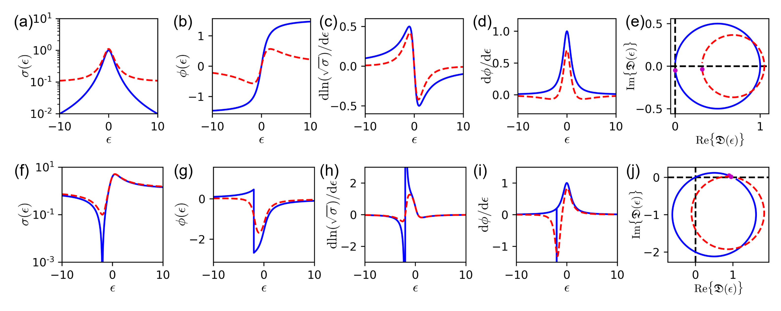
Figure 1: Transition amplitudes for the Lorentz and Fano resonances. Cross sections (a, f), phases (b, g), the derivatives of the logarithm of the cross sections (c, h), Wigner time delays (d, i), and transition-amplitude trajectories (e, j) for the Lorentzian lineshape (a-e) and the Fano lineshape with $q=2$ (f-j), respectively, where the blue solid lines correspond to $\sigma_{\rm a}=1$ and $\sigma_{\rm b}\rightarrow 0^{+}$, while the red dashed lines correspond to $\sigma_{\rm a}=1$ and $\sigma_{\rm b}=0.1$. The magenta dots in (e) and (f) indicate the beginning of the trajectories at $\epsilon\rightarrow-\infty$.

(Anti)resonances

The cross section of an (anti)resonance can be expressed by the Lorentzian lineshape, e.g., the Breit-Wigner resonance formula [66, 67]:

$$\sigma_{\rm L}(\epsilon)=\sigma_{\rm a}\frac{1}{\epsilon^{2}+1}+\sigma_{\rm b}$$ (13)

or the Fano lineshape [68, 69]:

$$\sigma_{\rm F}(\epsilon)=\sigma_{\rm a}\frac{{(\epsilon+q)}^{2}}{\epsilon^{2}+1}+\sigma_{\rm b},$$ (14)

where $\epsilon=(E-E_{\rm r})/(\Gamma/2)$ is the relative energy, and $\sigma_{\rm a}$ and $\sigma_{\rm b}$ are the resonant and non-resonant cross-sections, respectively. We assume that the corresponding pathways contribute to the overall transition amplitude coherently, which fits in the Feshbach picture [70] and was recently demonstrated in the x-ray regime [71]. The Lorentzian lineshape is symmetric, while the Fano lineshape is asymmetric, with $q$ being the asymmetric parameter. $\Gamma$ describes the peak width and thus the resonant state has a lifetime of $1/\Gamma$ from Fano’s picture. The cross section for a Lorentzian or Fano lineshape can be written as a common expression:

$$\sigma(\epsilon)=\mathfrak{S}\frac{(\epsilon+Q)^{2}+\gamma^{2}}{\epsilon^{2}+1}.$$ (15)

For the Lorentzian lineshape, $Q=0$, $\gamma^{2}=1+\sigma_{\rm a}/\sigma_{\rm b}$, where $\mathfrak{S}=\sigma_{\rm b}$, while for the Fano lineshape, $Q=q/(r+1)$, $\gamma^{2}=r(r+q^{2}+1)/(r+1)^{2}$, where $r={\sigma_{\rm b}/\sigma_{\rm a}}$, and $\mathfrak{S}=\sigma_{\rm a}+\sigma_{\rm b}$. The detailed proof can be found in Methods. Using $\partial/\partial E=(2/\Gamma)\partial/\partial\epsilon$, we have

$$\frac{1}{\sigma(E)}\frac{\partial\sigma}{\partial E}=\frac{2}{\Gamma}\left[\frac{\frac{2}{\gamma}\left(\frac{\epsilon+Q}{\gamma}\right)}{{\left(\frac{\epsilon+Q}{\gamma}\right)}^{2}+1}-\frac{2\epsilon}{\epsilon^{2}+1}\right].$$ (16)

It is easy to verify that the boundary condition (12) is fulfilled, and Eq. (10) yields

$$\tau(E)=\frac{2}{\Gamma}\left[-\frac{\frac{1}{|\gamma|}}{{\left(\frac{\epsilon+Q}{|\gamma|}\right)}^{2}+1}+\frac{1}{\epsilon^{2}+1}\right]\ .$$ (17)

Here we used the property of the Hilbert transform that $\mathcal{H}\{f(aE)\}(E)={\rm sgn}(a)[\mathcal{H}\{f(E)\}(aE)]$. The time delay can be decomposed as two Lorentzian lineshapes with widths of $\gamma\Gamma$ and $\Gamma$ and opposite signs, centered at $(E_{\rm r}-\frac{Q\Gamma}{2})$ and $E_{\rm r}$, respectively. For the Fano lineshape with $r\rightarrow 0$ and thus $|\gamma|\rightarrow 0$, the first time-delay peak approaches $-{\rm\pi}\delta(\epsilon+Q)$. On the other hand, for the Lorentzian lineshape with $\sigma_{\rm b}/\sigma_{\rm a}\rightarrow 0$ and thus $|\gamma|\rightarrow\infty$, the first time-delay peak vanishes and th the time delay is also a Lorentzian lineshape with $\tau(E_{\rm r})=2/\Gamma$, as discussed in [72].

Since $(Q+{\rm i}\gamma)$ can be regarded as the “complex asymmetry parameter” [71], a more insightful approach is to investigate the function [14, 73]

$$\mathfrak{D}(\epsilon)=\sqrt{\mathfrak{S}}\frac{\epsilon+Q+{\rm i}\gamma}{\epsilon+{\rm i}}=\sqrt{\mathfrak{S}}\left[1+\frac{Q+{\rm i}(\gamma-1)}{\epsilon+{\rm i}}\right].$$ (18)

It fulfills ${|\mathfrak{D}(\epsilon)|}^{2}=\sigma(\epsilon)$ and it is minimum-phase when $\gamma>0$, so the phase of the transition amplitude is the same as the phase of $\mathfrak{D}(\epsilon)$ with the freedom of a common phase shift, namely $D(\epsilon)=\mathfrak{D}(\epsilon){\rm e}^{{\rm i}\phi_{0}}$, and

$$\arg{\{D(\epsilon)\}}=\arg{\{\mathfrak{D}(\epsilon)\}}+\phi_{0}$$

$$=\arg{\{\epsilon+Q+{\rm i}\gamma\}}-\arg{\{\epsilon+{\rm i}\}}+\phi_{0}$$

$$=\cot^{-1}\left(\frac{\epsilon+Q}{\gamma}\right)-\cot^{-1}(\epsilon)+\phi_{0}.$$ (19)

Thus the Wigner time delay will be the same, as expressed in Eq. (17). The trajectory of $\mathfrak{D}(\epsilon)$ from $\epsilon\rightarrow-\infty$ to $\epsilon\rightarrow+\infty$ is a counter-clockwise rotating (due to the causality) closed circle [42, 14] with the radius of $\frac{\sqrt{\mathfrak{S}}}{2}\sqrt{{(\gamma-1)}^{2}+Q^{2}}$ centered at $\left(\sqrt{\mathfrak{S}}\frac{\gamma+1}{2},-\sqrt{\mathfrak{S}}\frac{Q}{2}\right)$. It can be easily verified that the origin is not enclosed when $\gamma>0$. Take the Fano resonance as an example, at $\epsilon\rightarrow\pm\infty$, the transition amplitudes are dominated by the direct ionisation channel, which is approximately constant in this region. As $r\rightarrow 0$ (“pure” Fano lineshape), the trajectory approaches tangential to the origin, where a $(-{\rm\pi})$-phase jump occurs within an infinitely small energy interval, which corresponds to the $-{\rm\pi}\delta(\epsilon+Q)$ peak. As $\gamma$ deviates from 0, the maximal phase jump is $2{\rm sgn}(\gamma-1){\cos}^{-1}\left(2\sqrt{\gamma}/\sqrt{{(\gamma+1)}^{2}+Q^{2}}\right)$ for $\gamma\neq 1$ and $\pm 2{\tan}^{-1}(Q/2)$ for $\gamma=1$ (see Methods for details). For the “pure” Lorentzian transition amplitude $D(\epsilon)\propto(\epsilon+{\rm i})^{-1}$ [42], there is a phase offset of ${\rm\pi}$ between $\epsilon\rightarrow+\infty$ and $\epsilon\rightarrow-\infty$, which does not fulfill the minimum-phase condition since it encloses “half” the origin. Its phase retrieved by the LHT method starts and ends at the same value at infinities, which corresponds to shifting the circle by an infinitely small amount away from the origin, and thus subtracts an infinitely broad Lorentzian lineshape according to Eq. (17), where $Q=0$ and $\gamma\rightarrow+\infty$. Its behavior near $\epsilon=0$, which is of most interest, is largely unchanged. The maximal phase jump is $4{\tan}^{-1}(\sqrt{\gamma})-\pi=4{\tan}^{-1}(\sqrt[4]{1+\sigma_{\rm a}/\sigma_{\rm b}})-\pi$, which approaches $\pi$ when $\sigma_{\rm a}/\sigma_{\rm b}\rightarrow 0$. Examples of Lorentzian and Fano lineshapes are plotted in Fig. 1, where the increase of $\sigma_{\rm b}/\sigma_{\rm a}$ results in the decrease of the extreme(s) of the time delay.

In preceding work [23] the shape-resonance analysis was performed by utilising the relation $\sigma_{\ell}(E)\propto\sin^{2}\phi_{\ell}$ from Eq. (5), which is applicable if only one $\ell$ is dominating. Assume that no background is contributing, and let $f_{l}(E)=-\cot[\phi_{l}(E)]$ be a real function, then

$$\sin^{2}[\phi_{l}(E)]=\frac{1}{{f_{l}(E)}^{2}+1}={\Big{|}\frac{1}{f_{l}(E)\pm{\rm i}}\Big{|}}^{2}.$$ (20)

Therefore, assuming $f_{l}(E)$ to be analytical,

$$\mathcal{H}\Bigl{\{}\frac{1}{2}\ln[\sigma_{l}(E)]\Bigr{\}}=-\arg\{f_{l}(E)\pm{\rm i}\}$$

$$=\mp\cot^{-1}[f_{l}(E)]=\pm\phi_{l}(E),$$ (21)

if one of the two branches $(f_{l}(E)\pm{\rm i})$ has no poles or zeros on the upper half-plane of $E$. For example, let $f_{l}(E)=(E-E_{{\rm r},l})/(\frac{\Gamma_{l}}{2})$, where $\Gamma_{l}>0$, $(f_{l}(E)+{\rm i})$ fulfills the condition and leads to the “pure” Breit-Wigner resonance with Lorentzian lineshape. For the Fano resonance, however, since the two branches cross at $\phi_{l}(E)=0$, where the cross section vanishes, the phase that fulfills the causality condition will be the combination of the two branches.

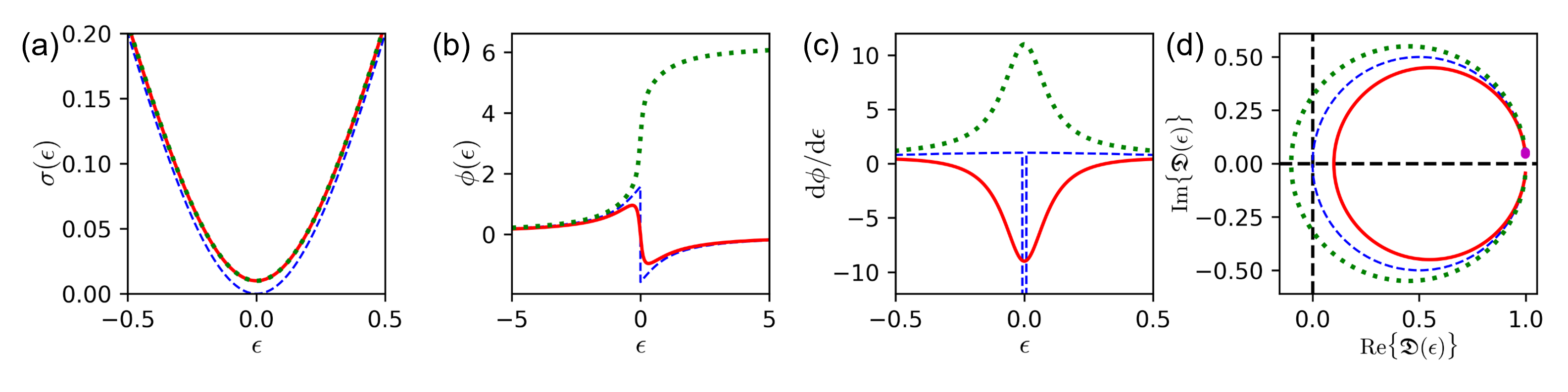
Figure 2: Comparison of the trajectories with different topologies. Cross sections in the vicinity of the minimum (a), phases (b), time delays (c), and trajectories (d, the magenta dot indicates $\epsilon\rightarrow-\infty$) of the anti-Lorentzian lineshapes with $\mathfrak{S}=1$ , $Q=0$ and $\gamma=0^{+}$ (blue, dashed), $0.1$ (red, solid), or $-0.1$ (green, dotted), according to Eq. (18).

In real experiments, the measurable energy range is finite and thus the boundary condition is not strictly fulfilled. This leads to a deviation of the retrieved time delay from its physical counterpart. However, when comparing two photoionisation processes, the relative time delay, which is usually the experimental observable [10], can be obtained from their cross-section ratio, which converges faster than the individual time delays:

$$\Delta\tau(E)=\tau_{1}(E)-\tau_{2}(E)=\frac{\partial}{\partial E}\arg\left\{\frac{D_{1}}{D_{2}}\right\}$$ (22)

$$= \frac{1}{2}\frac{\partial}{\partial E}\mathcal{H}\left\{\ln\left(\frac{\sigma_{1}}{\sigma_{2}}\right)\right\}=\frac{1}{2}\mathcal{H}\left\{\frac{\sigma_{2}}{\sigma_{1}}\frac{\partial(\sigma_{1}/\sigma_{2})}{\partial E}\right\}.$$

Time delays near Cooper minima

CM are antiresonances that have a distinctly different origin compared to the Fano or shape resonances [74, 75, 21]. Nevertheless, the cross section near the minimum can be locally fitted by a Fano lineshape with $\gamma\rightarrow 0$ in Eq. (15) (see Methods for details). Although $\pm\gamma$ give the same cross section, they have different topological structures on the complex plane. Only the transition amplitude corresponding to the positive $\gamma$ is minimum-phase, which leads to a negative time delay, while the negative $\gamma$ gives a positive time delay, as demonstrated in Fig. 2.

For numerical illustration of the proposed technique, we analyse the time delay near the CM in various shells of noble gas atoms: Xe $4d$, Ar $3p$ and Ar $3s$. The Xe $4d$ and Ar $3p$ CM have a kinematic origin where the radial node in the target orbital passes through the oscillation in the continuum radial orbital. The case of Ar $3s$ is different as the corresponding CM is induced by the inter-shell correlation with the $3p$ shell. These two different cases of kinematic and correlation induced CM allows us to demonstrate the utility of the proposed technique. Our numerical illustrations are based on the random-phase approximation with exchange (RPAE) calculations reported in [26]. First we evaluate the angle differential photoionisation cross-section (Complex photoionisation time delay and the Wigner time delay) in the zero emission direction $\hat{\bm{k}}\parallel\hat{\bm{e}}$. This cross-section in the vicinity of the CM is fitted with the standard set Fano parameters $E_{\rm r}$, $\Gamma$, $q$ and $\rho^{2}$ [68, 69, 76]. Next, these parameters are converted to an alternative set $Q$ and $\gamma$ which allows to express the photoionisation amplitude $D(E)$ (Eqs. (18, 19)) and the corresponding time delay $\tau(E)$ (Eq.(17)). These two quantities are compared with their numerical counterparts evaluated using the RPAE method.

This comparison is displayed in Fig. 3. Panels (a-c) show the photoionisation cross-sections near the corresponding CM. In panels (d-f), the parametric plots exhibit the complex photoionisation amplitudes $\mathfrak{D}(E)$ as given analytically by Eq. (18) and evaluated in the RPAE, respectively. The arrows in the amplitude graphs indicate the winding direction as the photon energy increases. In (g-i), we display the corresponding time delays. The three columns, from left to right, correspond to the Xe $4d$, Ar $3p$ and Ar $3s$ orbitals, respectively. The LHT-extracted time delays given by Eq. (14) show very good agreement with the numeric results for Xe $4d$ and Ar $3p$, while for the Ar $3s$ CM there is a qualitative disagreement that LHT yields negative delay at the cross-section minimum, while the computation suggests the opposite. Such a profound difference in time delays near the CM can be traced to the corresponding photoionisation amplitudes and their winding numbers, as plotted in panels (d-f). In the cases of Xe $4d$ and Ar $3p$, both the analytic and numeric amplitudes do not encircle the origin and their respective winding numbers are 0. The case of Ar $3s$ is different where the RPAE amplitude encircles the origin, namely, the minimum-phase condition is not fulfilled. In Eq. (18), when $\gamma<0$, the transition amplitude, denoted as $\breve{D}(\epsilon)$, has a zero at $(-Q+{\rm i}|\gamma|)$ and thus has winding number of 1. The LHT-retrieved transition amplitude can be expressed as

$$\mathfrak{D}(\epsilon)=\frac{\epsilon+Q+{\rm i}|\gamma|}{\epsilon+Q-{\rm i}|\gamma|}\breve{D}(\epsilon){\rm e}^{{\rm i}\phi_{0}},$$ (23)

which gives rise to a Lorentzian lineshape that should be added to the LHT-retrieved time delay:

$$\frac{\partial\arg\{\breve{D}(\epsilon)\}}{\partial\epsilon}=\frac{\partial\arg\{\mathfrak{D}(\epsilon)\}}{\partial\epsilon}+\frac{\frac{2}{|\gamma|}}{{\left(\frac{\epsilon+Q}{|\gamma|}\right)}^{2}+1}.$$ (24)

Hence, Eq. (17) becomes

$$\breve{\tau}(E)=\frac{2}{\Gamma}\left[\frac{\frac{1}{|\gamma|}}{{\left(\frac{\epsilon+Q}{|\gamma|}\right)}^{2}+1}+\frac{1}{\epsilon^{2}+1}\right],$$ (25)

which turns the negative peak into a positive peak, and in the limit of $\gamma\rightarrow 0^{-}$, it becomes the $+{\rm\pi}\delta(\epsilon+Q)$ peak. The time delays near the CM for the zero-winding-number and one-winding-number trajectories are given by Eq. (17) and Eq. (25), respectively. Using Eqs. (23, 25), the complex transition amplitude and the corresponding time delay of the Ar $3s$ CM with winding number equalling to 1 can be retrieved, as shown in panels (f) and (i) in Fig. 3, respectively. This gives a positive time delay that excellently agrees with the RPAE result, which indicates that the KK relations reduces the detailed time-delay computation into the quantitative winding-number determination, as long as the cross section is available experimentally or theoretically. The RABBIT measurement reported in [77] suggests that the time delay of Ar $3s$ CM is more negative than that of Ar $3p$, which contradicts the theoretical calculation. As compared in Fig. 4, with the fitted Fano parameters from the computed cross sections, assuming that Ar $3s$ has winding number of 1 at CM, the retrieved relative time delay between Ar $3s$ and $3p$ matches the computation, while assuming that Ar $3s$ has winding number of 0 at CM leads to a better agreement with the measured values which strikingly deviate from the theoretical prediction with the opposite sign. This indicates that the other pathways, e.g. the shake-up channels, shift the trajectory near the origin, so that the winding number changes from 1 to 0 and leads to a negative delay.

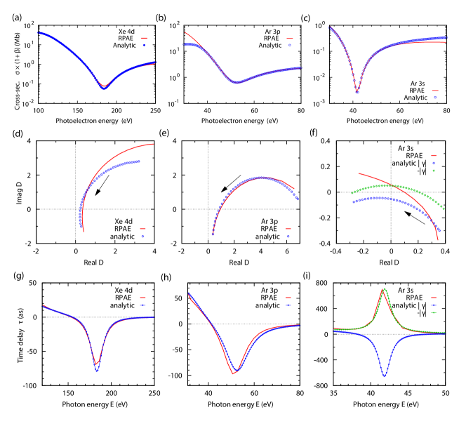
Figure 3: Comparison of the cross-section-time-delay relation of various CM. The photoionisation cross-sections in the CM of Xe $4d$ (a), Ar $3p$ (b), and Ar $3s$ (c) from the RPAE calculations (solid red) are fitted with the Fano lineshape Eq. (14) (blue dots). The photoionisation amplitudes of Xe $4d$ (d), Ar $3p$ (e), and Ar $3s$ (f) computed by RPAE and reconstructed from the Fano profile using Eq. (18) are compared. The corresponding time delays from RPAE and by the analytic formula in Eq. (3) are shown in (g-i). For Ar $3s$ the effect of the sign of the parameter $\pm|\gamma|$ is illustrated in (f) and (i), where the blue dots correspond to Eq. (14) and the green dots correspond to Eq. (25).

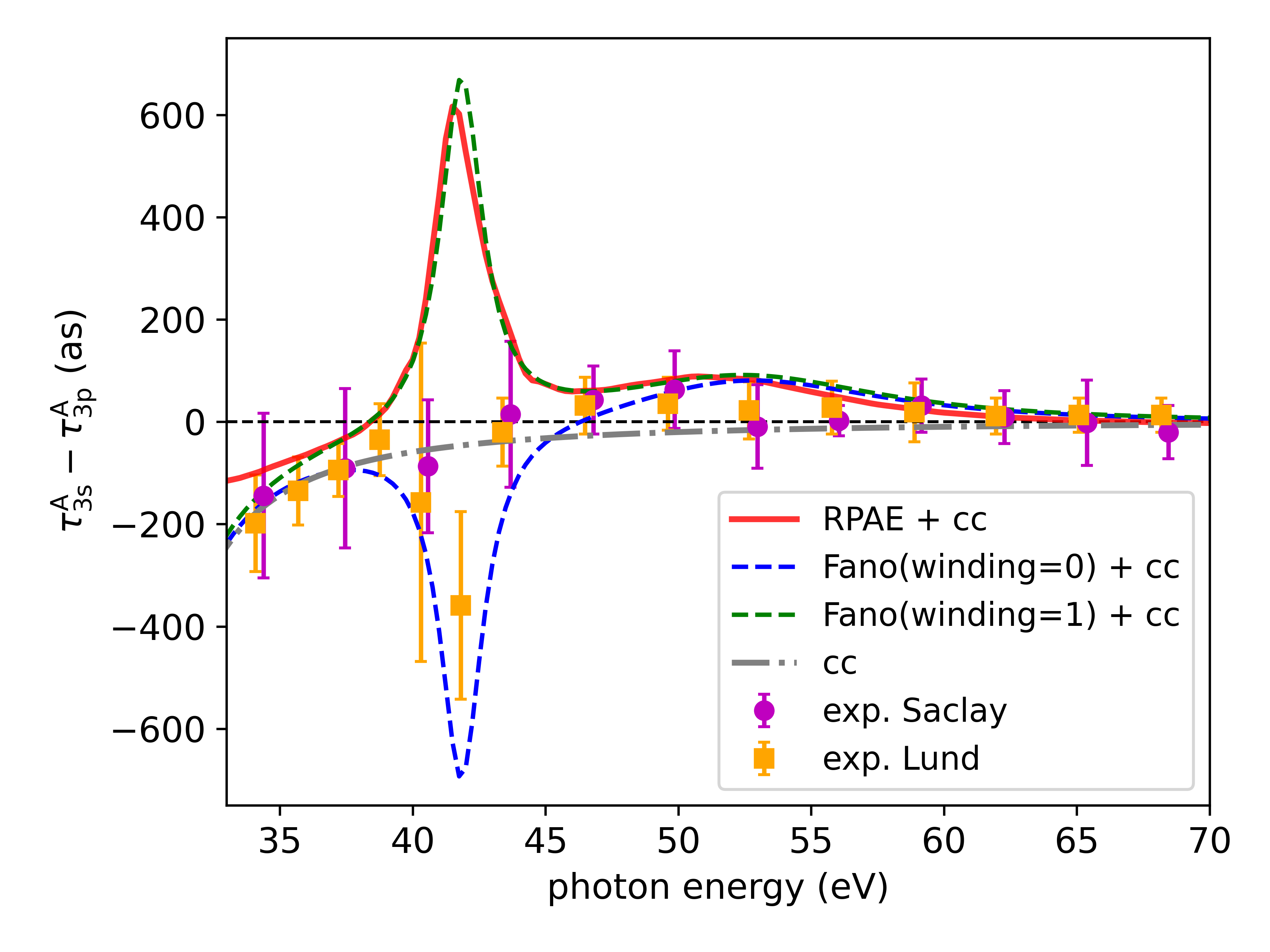
Figure 4: Experimental[77] and computed (RPAE, same as in Fig. 3) relative time delays between argon $3s$ and $3p$, compared with the time delay retrieved from the Fano parameters using Eqs. (17, 25). The contribution from the continuum-continuum (cc) transition due to the dressing IR field in the RABBIT measurement is addressed by adding an additional cc time delay given in [78].

Conclusions

In conclusion, we have introduced a Kramers-Kronig-like relation between photoionisation cross section and attosecond time delays, which relies on the general properties of coherence and causality of the transition amplitude. We have derived a unified time-delay formula of Lorentzian and Fano lineshapes with constant and coherent background, where both Breit-Wigner and Fano resonances correspond to a pair of Lorentzian time-delay peaks with opposite signs. We analysed several cases of the CM in valence shells of noble gas atoms. The relation is manifested by the excellent agreement of the retrieved time delays near CM of Xe $4d$ and Ar $3p$ from the their cross sections, in comparison to the calculated time delay by RPAE. The LHT further requires the topological structure that the trajectory has winding number of 0, which is particularly relevant for antiresonances where the minimal cross section approaches zero. While the cases of Xe $4d$ and Ar $3p$ display clearly the winding number of 0, the case of Ar $3s$ remains controversial with the analytic winding number of 0 being different from the numeric winding number of 1. The latest experimental results [77] rather hint at a negative time delay near the CM of Ar $3s$, which is at variance with the RPAE [26] and TDLDA [29] predictions. So this particular case remains controversial and suggests a need for additional investigations.

We note that our method is not restricted to atomic one-photon processes, since similar resonances have been found in molecular systems [17, 19, 20, 24] and in two-photon transitions [79, 80, 73, 18]. Our result bridges two kinds of experiments in atomic and molecular physics and broadens the understanding of attosecond processes.

Methods

Formulation of the Lorentzian peak and the Fano peak

The Lorentzian line shape is given by

$$\sigma=\sigma_{\rm a}\frac{1}{\epsilon^{2}+1}+\sigma_{\rm b}=\sigma_{\rm b}\frac{\epsilon^{2}+1+{\sigma_{\rm a}/\sigma_{\rm b}}}{\epsilon^{2}+1}.$$ (26)

Compared with Eq. (15), we have $\mathfrak{S}=\sigma_{\rm b}$, $Q=0$, and $\gamma^{2}=1+\sigma_{\rm a}/\sigma_{\rm b}$. For the Fano line shape,

$$\sigma=\sigma_{\rm a}\frac{{(\epsilon+q)}^{2}}{\epsilon^{2}+1}+\sigma_{\rm b}=(\sigma_{\rm a}+\sigma_{\rm b})\frac{\epsilon^{2}+\frac{2q\epsilon+q^{2}+r}{r+1}}{\epsilon^{2}+1}.$$ (27)

Compared with Eq. (15), we have $\mathfrak{S}=\sigma_{\rm a}+\sigma_{\rm b}$, $2Q=\frac{2q}{r+1}$ and $Q^{2}+\gamma^{2}=\frac{q^{2}+r}{r+1}$, which leads to the expressions in the main text. From Eq. (15) we have

$$\frac{1}{\sigma}\frac{\partial\sigma}{\partial\epsilon} =\frac{2(\epsilon+Q)(\epsilon^{2}+1)-[{(\epsilon+Q)}^{2}+\gamma^{2}]\cdot 2\epsilon}{[{(\epsilon+Q)}^{2}+\gamma^{2}](\epsilon^{2}+1)}$$ (28)

$$=\frac{2\left(\epsilon+Q\right)}{{\left(\epsilon+Q\right)}^{2}+\gamma^{2}}-\frac{2\epsilon}{\epsilon^{2}+1},$$

which yields Eq. (16).

Phase-jump calculation

For $\mathfrak{D}(\epsilon)$ in Eq. (18), we have

$${\rm Re}\{\mathfrak{D}(\epsilon)\}/\sqrt{\mathfrak{S}} =\frac{\epsilon^{2}+Q\epsilon+\gamma}{\epsilon^{2}+1},$$

$${\rm Im}\{\mathfrak{D}(\epsilon)\}/\sqrt{\mathfrak{S}} =\frac{(\gamma-1)\epsilon-Q}{\epsilon^{2}+1}.$$ (29)

It can be verified that

$${\left(\frac{{\rm Re}\{\mathfrak{D}(\epsilon)\}}{\sqrt{\mathfrak{S}}}-\frac{\gamma+1}{2}\right)}^{2}+{\left(\frac{{\rm Im}\{\mathfrak{D}(\epsilon)\}}{\sqrt{\mathfrak{S}}}+\frac{Q}{2}\right)}^{2}$$

$$=\frac{1}{4}\left[{(\gamma-1)}^{2}+Q^{2}\right].$$ (30)

Hence, the trajectory of $\mathfrak{D}(\epsilon)$ is a circle with the radius of $\frac{\sqrt{\mathfrak{S}}}{2}\sqrt{{(\gamma-1)}^{2}+Q^{2}}$ centered at $\left(\sqrt{\mathfrak{S}}\frac{\gamma+1}{2},-\sqrt{\mathfrak{S}}\frac{Q}{2}\right)$. Since the origin is $\frac{\sqrt{\mathfrak{S}}}{2}\sqrt{{(\gamma+1)}^{2}+Q^{2}}$ away from the center of the circle, the tangent segment from the origin is $\sqrt{\mathfrak{S}}\sqrt{\gamma}$, and the angle between the two tangents yields

$${|\Delta\phi|}_{\max} =\max(\phi(\epsilon))-\min(\phi(\epsilon))$$ (31)

$$=2{\cos}^{-1}\left(\frac{2\sqrt{\gamma}}{\sqrt{{(\gamma+1)}^{2}+Q^{2}}}\right).$$

At $\epsilon\rightarrow-\infty$, the starting point of the trajectory approaches $(\sqrt{\mathfrak{S}},0)$, which is left to the center when $\gamma>1$ while right to the center when $\gamma<1$. Since the trajectory evolves counter-clockwise, the phase between the two tangents increases when $\gamma>0$ and decreases when $\gamma<0$. Therefore, the phase jump for $\gamma\neq 1$ can be expressed as

$${\Delta\phi}_{\max}=2{\rm sgn}(\gamma-1){\cos}^{-1}\left(\frac{2\sqrt{\gamma}}{\sqrt{{(\gamma+1)}^{2}+Q^{2}}}\right).$$ (32)

For $\gamma=1$, it corresponds to a symmetric phase variation, where the maximal (minimal) phase is at $\epsilon=0$ while the minimal (maximal) phase is at $\epsilon=\pm\infty$, and

$$\phi^{\gamma=1}(0)-\phi^{\gamma=1}(\infty) =-2{\rm sgn}(Q){\cos}^{-1}\left(\frac{1}{\sqrt{1+{(Q/2)}^{2}}}\right)$$ (33)

$$=-2{\tan}^{-1}(Q/2).$$

In the special case of $Q=0$, namely the Lorentzian peak, the expression can be simplified to

$${\Delta\phi}^{Q=0}_{\max}=4{\tan}^{-1}(\sqrt{\gamma})-\pi,$$ (34)

which is positive when $\gamma>1$ (maximum in cross section) and is negative when $\gamma<1$ (minimum in cross section). It approaches $+{\rm\pi}$ and $-{\rm\pi}$ for $\gamma\rightarrow+\infty$ ($\sigma_{\rm b}/\sigma_{\rm a}\rightarrow-1$) and $\gamma\rightarrow 0$ ($\sigma_{\rm b}/\sigma_{\rm a}\rightarrow 0$), respectively.

RPAE calculation

The RPAE calculations were performed using the atom program suite [81]. For argon, the correlations between the three optically allowed transitions $3s\to Ep$ and $3p\to Es/Ed$ were taken into account. For Xe $4d$, the five transitions $5s\to Ep$, $4p\to Es/Ed$ and $4d\to Ep/Ef$ were included. The cross-section in the polarization direction was was evaluated from the total photoionization cross-section and the angular anisotropy parameter as $\sigma(1+\beta)$. The length gauge results were used for both $\sigma$ and $\beta$. The time delay in the polarization direction was evaluated from the photoionization amplitude as in [26]. Summation over the magnetic projections in the ground state was reduced to $m_{i}=0$.

Fano parameters for cross sections near Cooper minima

The cross section of a Fano resonance can be conventionally expressed as [68, 69, 76]:

$$\sigma_{\rm F}(\epsilon)=\sigma_{0}(\epsilon)\left(\rho^{2}\frac{{(q+\epsilon)}^{2}}{1+\epsilon^{2}}+1-\rho^{2}\right),$$ (35)

where $\epsilon=(E-E_{\rm r})/(\Gamma/2)$, and $\rho^{2}$ is known as the correlation coefficient, and it is linked to Eq. (14) by letting $\sigma_{\rm a}=\rho^{2}\sigma_{0}$, $\sigma_{\rm b}=(1-\rho^{2})\sigma_{0}$, $r=\sigma_{\rm b}/\sigma_{\rm a}=1/{\rho^{2}}-1$, and approximating $r$ as a constant across the CM. From the RPAE calculation, the Fano parameters are $E_{\rm r}=105.46\leavevmode\nobreak\ {\rm eV}$, $\Gamma=64.0282\leavevmode\nobreak\ {\rm eV}$, $\sigma_{0}=6.26653\leavevmode\nobreak\ {\rm Mb}$, $q=-2.45287$, $\rho^{2}=0.990963$ for Xe $4d$ CM, $E_{\rm r}=29.2918\leavevmode\nobreak\ {\rm eV}$, $\Gamma=18.468\leavevmode\nobreak\ {\rm eV}$, $\sigma_{0}=8.62031\leavevmode\nobreak\ {\rm Mb}$, $q=-2.67896$, $\rho^{2}=0.934333$ for Ar $3p$ CM, and $E_{\rm r}=31.4118\leavevmode\nobreak\ {\rm eV}$, $\Gamma=19.6322\leavevmode\nobreak\ {\rm eV}$, $\sigma_{0}=0.567772\leavevmode\nobreak\ {\rm Mb}$, $q=-1.06661$, $\rho^{2}=0.995518$ for Ar $3s$ CM, respectively, which correspond to the fitted curves in Fig. 3.

Author contributions statement

J.-B.J. derived the formulae with support of A.S.K., M.H., and K.U. A.S.K. performed the RPAE calculation and the fitting. J.-B.J., K.U., and H.J.W. conceived the study. M.H., K.U., and H.J.W. supervised its realization. All authors discussed the results and wrote the paper.

Competing interests statement

All co-authors have seen and agree with the contents of the manuscript and there is no financial interest to report.

References

- [1] Becker, U. & Shirley, D. A. VUV and Soft X-ray Photoionization (Plenum Press, 1996).
- [2] Schmidt, V. Electron Spectrometry of Atoms using Synchrotron Radiation. Cambridge Monographs on Atomic, Molecular and Chemical Physics (Cambridge University Press, 1997).
- [3] Corkum, P. B. & Krausz, F. Attosecond science. \JournalTitleNature Physics 3, 381–387 (2007).
- [4] Krausz, F. & Ivanov, M. Attosecond physics. \JournalTitleRev. Mod. Phys. 81, 163–234 (2009).
- [5] Itatani, J. et al. Attosecond streak camera. \JournalTitlePhys. Rev. Lett. 88, 173903 (2002).
- [6] Kienberger, R. et al. Atomic transient recorder. \JournalTitleNature 427, 817–821 (2003).
- [7] Véniard, V., Taïeb, R. & Maquet, A. Phase dependence of (n+1)-color (n>1) ir-uv photoionization of atoms with higher harmonics. \JournalTitlePhysical Review. A 54, 721–728, DOI: 10.1103/PhysRevA.54.721 (1996).
- [8] Paul, P. M. et al. Observation of a train of attosecond pulses from high harmonic generation. \JournalTitleScience 292, 1689 (2001).
- [9] Schultze, M. et al. Delay in photoemission. \JournalTitleScience 328, 1658–1662 (2010).
- [10] Klünder, K. et al. Probing single-photon ionization on the attosecond time scale. \JournalTitlePhysical Review Letters 106, 143002, DOI: 10.1103/PhysRevLett.106.143002 (2011).
- [11] Eisenbud, L. The formal properties of nuclear collisions (Princeton University, 1948).
- [12] Wigner, E. P. Lower limit for the energy derivative of the scattering phase shift. \JournalTitlePhysical Review 98, 145 (1955).
- [13] Smith, F. T. Lifetime matrix in collision theory. \JournalTitlePhysical Review 118, 349 (1960).
- [14] Kotur, M. et al. Spectral phase measurement of a fano resonance using tunable attosecond pulses. \JournalTitleNature Communications 7, 1–6 (2016).
- [15] Gruson, V. et al. Attosecond dynamics through a fano resonance: Monitoring the birth of a photoelectron. \JournalTitleScience 354, 734–738, DOI: 10.1126/science.aah5188 (2016).
- [16] Zhong, S. et al. Attosecond electron–spin dynamics in xe 4d photoionization. \JournalTitleNature Communications 11, 1–6 (2020).
- [17] Huppert, M., Jordan, I., Baykusheva, D., Von Conta, A. & Wörner, H. J. Attosecond delays in molecular photoionization. \JournalTitlePhysical Review Letters 117, 093001 (2016).
- [18] Baykusheva, D. & Wörner, H. J. Theory of attosecond delays in molecular photoionization. \JournalTitleThe Journal of Chemical Physics 146, 124306, DOI: 10.1063/1.4977933 (2017).
- [19] Heck, S. et al. Attosecond interferometry of shape resonances in the recoil frame of cf4. \JournalTitleScience Advances 7, eabj8121 (2021).
- [20] Nandi, S. et al. Attosecond timing of electron emission from a molecular shape resonance. \JournalTitleScience Advances 6, eaba7762 (2020).
- [21] Schoun, S. et al. Attosecond pulse shaping around a cooper minimum. \JournalTitlePhysical Review Letters 112, 153001 (2014).
- [22] Heck, S. et al. Two-center interference in the photoionization delays of kr 2. \JournalTitlePhysical Review Letters 129, 133002 (2022).
- [23] Kheifets, A. S. & Catsamas, S. Shape resonances in photoionization cross sections and time delay. \JournalTitlePhysical Review A 107, L021102 (2023).
- [24] Holzmeier, F. et al. Influence of shape resonances on the angular dependence of molecular photoionization delays. \JournalTitleNature Communications 12, 1–9 (2021).
- [25] Guenot, D. et al. Photoemission-time-delay measurements and calculations close to the 3 s-ionization-cross-section minimum in ar. \JournalTitlePhysical Review A 85, 053424 (2012).
- [26] Kheifets, A. Time delay in valence-shell photoionization of noble-gas atoms. \JournalTitlePhysical Review A 87, 063404 (2013).
- [27] Dixit, G., Chakraborty, H. S. & Madjet, M. E.-A. Time delay in the recoiling valence photoemission of ar endohedrally confined in c60. \JournalTitlePhysical Review Letters 111, 203003 (2013).
- [28] Pi, L.-W. & Landsman, A. S. Attosecond time delay in photoionization of noble-gas and halogen atoms. \JournalTitleApplied Sciences 8, 322 (2018).
- [29] Magrakvelidze, M., Madjet, M. E.-A., Dixit, G., Ivanov, M. i. & Chakraborty, H. S. Attosecond time delay in valence photoionization and photorecombination of argon: A time-dependent local-density-approximation study. \JournalTitlePhys. Rev. A 91, 063415 (2015).
- [30] Hilborn, R. C. Einstein coefficients, cross sections, f values, dipole moments, and all that. \JournalTitleAmerican Journal of Physics 50, 982–986 (1982).
- [31] Natalense, A. P. P. & Lucchese, R. R. Cross section and asymmetry parameter calculation for sulfur 1s photoionization of sf6. \JournalTitleJ. Chem. Phys. 111, 5344–5348 (1999).
- [32] Pazourek, R., Nagele, S. & Burgdörfer, J. Attosecond chronoscopy of photoemission. \JournalTitleReviews of Modern Physics 87, 765 (2015).
- [33] Wigner, E. P. & Eisenbud, L. Higher angular momenta and long range interaction in resonance reactions. \JournalTitlePhysical Review 72, 29 (1947).
- [34] Kelkar, N. & Nowakowski, M. Analysis of averaged multichannel delay times. \JournalTitlePhysical Review A 78, 012709 (2008).
- [35] Schützer, W. & Tiomno, J. On the connection of the scattering and derivative matrices with causality. \JournalTitlePhysical Review 83, 249 (1951).
- [36] Van Kampen, N. S matrix and causality condition. ii. nonrelativistic particles. \JournalTitlePhysical Review 91, 1267 (1953).
- [37] Gell-Mann, M., Goldberger, M. & Thirring, W. E. Use of causality conditions in quantum theory. \JournalTitlePhysical Review 95, 1612 (1954).
- [38] Goldberger, M. L. Use of causality conditions in quantum theory. \JournalTitlePhysical Review 97, 508 (1955).
- [39] Karplus, R. & Ruderman, M. A. Applications of causality to scattering. \JournalTitlePhysical Review 98, 771 (1955).
- [40] Khuri, N. N. Analyticity of the schrödinger scattering amplitude and nonrelativistic dispersion relations. \JournalTitlePhysical Review 107, 1148 (1957).
- [41] Meiman, M. The causality principle and asymptotic behavior of the scattering amplitude. \JournalTitleSov. Phys. JETP 47, 188 (1964).
- [42] Taylor, J. R. Scattering theory: the quantum theory of nonrelativistic collisions (John Wiley & Sons, Inc., 1972).
- [43] Rescigno, T. N. & Reinhardt, W. P. Calculation of substituted fredholm determinants using complex basis functions. \JournalTitlePhysical Review A 8, 2828 (1973).
- [44] Reinhardt, W. P. Complex coordinates in the theory of atomic and molecular structure and dynamics. \JournalTitleAnnual Review of Physical Chemistry 33, 223–255 (1982).
- [45] Moiseyev, N. Quantum theory of resonances: calculating energies, widths and cross-sections by complex scaling. \JournalTitlePhysics Reports 302, 212–293 (1998).
- [46] Branson, D. Time and the s matrix. \JournalTitlePhysical Review 135, B1255 (1964).
- [47] Eden, R. & Landshoff, P. The problem of causality in s-matrix theory. \JournalTitleAnnals of Physics 31, 370–390 (1965).
- [48] Peres, A. Causality in s-matrix theory. \JournalTitleAnnals of Physics 37, 179–208 (1966).
- [49] Kramers, H. A. The law of dispersion and bohr’s theory of spectra. \JournalTitleNature 113, 673–674 (1924).
- [50] de L. Kronig, R. On the theory of dispersion of x-rays. \JournalTitleJ. Opt. Soc. Am. 12, 547–557, DOI: 10.1364/JOSA.12.000547 (1926).
- [51] Kramers, H. A. La diffusion de la lumière par les atomes. In Atti Cong. Intern. Fisica (Transactions of Volta Centenary Congress) Como, vol. 2, 545–557 (1927).
- [52] Abbamonte, P., Finkelstein, K., Collins, M. & Gruner, S. Imaging density disturbances in water with a 41.3-attosecond time resolution. \JournalTitlePhysical Review Letters 92, 237401 (2004).
- [53] Ott, C. et al. Lorentz meets fano in spectral line shapes: a universal phase and its laser control. \JournalTitleScience 340, 716–720 (2013).
- [54] Stooß, V. et al. Real-time reconstruction of the strong-field-driven dipole response. \JournalTitlePhysical Review Letters 121, 173005 (2018).
- [55] Lee, Y.-W. Synthesis of electric networks by means of the fourier transforms of laguerre’s functions. \JournalTitleJournal of Mathematics and Physics 11, 83–113 (1932).
- [56] Bode, H. W. et al. Network analysis and feedback amplifier design (van Nostrand, 1945).
- [57] Raymond, F.-H. Transformées de hilbert et relations de bayard-bode. In Annales Des Télécommunications, vol. 6, 262–272 (Springer, 1951).
- [58] Hoenders, B. On the solution of the phase retrieval problem. \JournalTitleJournal of Mathematical Physics 16, 1719–1725 (1975).
- [59] Burge, R., Fiddy, M., Greenaway, A. & Ross, G. The phase problem. \JournalTitleProceedings of the Royal Society of London. A. Mathematical and Physical Sciences 350, 191–212 (1976).
- [60] Mecozzi, A. Retrieving the full optical response from amplitude data by hilbert transform. \JournalTitleOptics Communications 282, 4183–4187 (2009).
- [61] Mecozzi, A. A necessary and sufficient condition for minimum phase and implications for phase retrieval. \JournalTitlearXiv preprint arXiv:1606.04861 DOI: 10.48550/arxiv.1606.04861 (2016).
- [62] Shilov, G. E. Convergence of Improper Integrals, 438–443. Dover books on mathematics (Dover Publications, New York, 1996), revised english edn.
- [63] Zorich, V. A. Integrals Depending on a Parameter, 405–492 (Springer Berlin Heidelberg, Berlin, Heidelberg, 2016).
- [64] Pollak, E. & Miller, W. H. New physical interpretation for time in scattering theory. \JournalTitlePhysical Review Letters 53, 115 (1984).
- [65] Yamada, N. Unified derivation of tunneling times from decoherence functionals. \JournalTitlePhysical Review Letters 93, 170401 (2004).
- [66] Breit, G. & Wigner, E. Capture of slow neutrons. \JournalTitlePhysical Review 49, 519 (1936).
- [67] Friedrich, H. Theoretical atomic physics (Springer International Publishing, 2017).
- [68] Fano, U. Effects of configuration interaction on intensities and phase shifts. \JournalTitlePhysical Review 124, 1866 (1961).
- [69] Fano, U. & Cooper, J. Line profiles in the far-uv absorption spectra of the rare gases. \JournalTitlePhysical Review 137, A1364 (1965).
- [70] Feshbach, H. A unified theory of nuclear reactions. ii. \JournalTitleAnnals of Physics 19, 287–313 (1962).
- [71] Ma, Z.-R. et al. First observation of new flat line fano profile via an x-ray planar cavity. \JournalTitlePhysical Review Letters 129, 213602 (2022).
- [72] Goldberger, M. L. & Watson, K. M. Concerning the notion of "time interval" in s-matrix theory. \JournalTitlePhysical Review 127, 2284 (1962).
- [73] Argenti, L. et al. Control of photoemission delay in resonant two-photon transitions. \JournalTitlePhysical Review A 95, 043426 (2017).
- [74] Cooper, J. W. Photoionization from outer atomic subshells. a model study. \JournalTitlePhys. Rev. 128, 681 (1962).
- [75] Wörner, H. J., Niikura, H., Bertrand, J. B., Corkum, P. B. & Villeneuve, D. M. Observation of electronic structure minima in high-harmonic generation. \JournalTitlePhysical Review Letters 102, 103901 (2009).
- [76] Kossmann, H., Krassig, B. & Schmidt, V. New determination of beutler-fano parameters for the 3s3p 1p1 resonance in helium. \JournalTitleJournal of Physics B: Atomic, Molecular and Optical Physics 21, 1489 (1988).
- [77] Alexandridi, C. et al. Attosecond photoionization dynamics in the vicinity of the cooper minima in argon. \JournalTitlePhysical Review Research 3, L012012 (2021).
- [78] Dahlström, J. M. & Lindroth, E. Study of attosecond delays using perturbation diagrams and exterior complex scaling. \JournalTitleJournal of Physics B: Atomic, Molecular and Optical Physics 47, 124012 (2014).
- [79] Jiménez-Galán, Á., Argenti, L. & Martín, F. Modulation of attosecond beating in resonant two-photon ionization. \JournalTitlePhysical Review Letters 113, 263001 (2014).
- [80] Jiménez-Galán, Á., Martín, F. & Argenti, L. Two-photon finite-pulse model for resonant transitions in attosecond experiments. \JournalTitlePhysical Review A 93, 023429 (2016).
- [81] Amusia, M. I. & Chernysheva, L. V. Computation of atomic processes : A handbook for the ATOM programs (Institute of Physics Pub., Bristol, UK, 1997).
Acknowledgements
J.-B.Ji acknowledges the funding from the ETH grant 41-20-2. M.H.’s work was funded by the European Union’s Horizon 2020 research and innovation programme under Marie Skłodowska-Curie agreement grant No. 801459, FP-RESOMUS. J.-B.Ji thanks Prof. Dr. J. O. Richardson (ETH Zürich) and Prof. Dr. R. R. Lucchese (Lawrence Berkeley National Laboratory) for discussions.