Constant-roll and primordial black holes in $f(Q,T)$ gravity

Abstract

In this study, we investigate the consequence of the constant-roll condition and examine the role of $f(Q,T)$ gravity in the cosmological inflation process. We analyze the inflationary scenario by calculating modified Friedmann equations, and giving an alternative technique that enables relating modified slow-roll parameters to the constant roll parameter $\beta$. Considering both chaotic and hilltop models, we calculate the spectral index and the tensor-to-scalar ratio and compare their compatibility with Planck’s data for different choices of the constant roll parameter $\beta$. We examine the evolution of primordial black holes in our chosen modified gravity model taking into account the accretion process and the evaporation due to Hawking radiation. We compute the evaporation and accretion masses rate and provide an analytic estimation of the primordial black holes masse and of the radiation in the $f(Q,T)$ gravity model.

I Introduction

Inflationary cosmology, or simply inflation, is the current widely accepted paradigm for explaining the physics of very early Universe. In this theory a quasi-exponential accelerating phase before the radiation decelerating era is proposed to solve the several long-standing puzzles of the Hot Big-Bang standard cosmological model [1, 2, 3, 4]. In addition, the most fascinating feature of inflation is that it provides a mechanism to explain the origin of the Cosmic Microwave Background (CMB) temperature anisotropies and the Large-Scale Structure (LSS) [6], and the subsequent phases at which matter appeared for the first time in the Universe [5]. The mechanism of inflation is based on the generation of small quantum fluctuations in the inflaton field, which is the field driving the accelerated expansion. These quantum fluctuations are amplified in physical scale during inflation, leading to a Gaussian, scale-invariant and adiabatic primordial density perturbations [6, 7]. This information is encoded into the primordial scalar power spectrum $\mathcal{P}_{s}$ and its scale dependence is characterized by the scalar spectral index $n_{s}$, which is tightly constrained by the latest Planck data [8] to be $n_{s}=0.9649\pm 0.0042$ (at $68\%$ C.L.). Furthermore, inflation also predicts the generation of tensor perturbations as a background of primordial gravitational waves (PGWs) [9, 10, 11]. In this case the amplitude of the primordial tensor power spectrum $\mathcal{P}_{t}$ can be parameterized in terms of the tensor-to-scalar ratio $r\equiv\mathcal{P}_{t}/\mathcal{P}_{s}$ [12]. Although no primordial gravitational waves have been detected so far, current observations give us an upper bound on $r$. New data from BICEP/Keck 2021 [13] have been published, leading to a considerably stronger upper bound on r: $r_{0.05}=0.014_{-0.011}^{+0.010}$ ($r_{0.05}<0.036$ (at $95\%$ C.L.)), in comparison to Planck $2018$ data [8].

In general, the dynamics of inflation is based on the slow-roll approximation. The scalar potential is chosen to be flat such that the scalar field slowly rolls down the potential [6]. So, the equation of the mode functions associated to quantum fluctuations can be written as a Bessel equation of order $\nu$, and $\nu$ is approximated to the first order of the Hubble slow-roll parameters $\epsilon_{H}\ll 1$ and $\eta_{H}\ll 1$. Thus, the mode functions and the corresponding power spectra are obtained by applying the so-called Bessel function approximation [14]. However, another alternative that has already been considered in the literature is the case of ultra-slow roll inflation [15, 16, 17]. The scalar potential is assumed to be extremely flat, and then the Klein-Gordon equation of motion of the homogeneous inflaton field is simplified by neglecting the slope term. Therefore, the friction term is now locked with the acceleration term. Furthermore, one has that $\eta_{H}\approx 3$ and then the slow-roll approximation is no longer valid. For instance, the mechanism to generate primordial black holes within the framework of ultra-slow roll inflation has been investigated in Refs. [100, 101]. Ultra-slow roll inflation has also been generalized to constant-roll inflation such that the slow-roll parameter $\eta_{H}$ becomes a constant [114, 113] (see also Refs. [18, 19, 20, 21, 22, 23]). Interestingly enough, constant-roll inflation differs from slow-roll inflation due to its new dynamical features that result in richer physics. It gives rise to a large local non-Gaussianity and the curvature perturbation may grow on the super-horizon scales [114, 113, 24].

Primordial Black Holes (PBHs) [25] started to be considered seriously after Hawking proposed that PBHs could be formed with Planck-order masses in the early Universe [26]. In this direction one would consider that PBHs formation could be a result of inflation [27] inhomogeneities from the early Universe [28, 29] or the phase transition [30]. Furthermore, it was first proposed that PBHs could be a candidate of dark matter (DM) in [31] and reconsidered in [32, 33] when black holes mergers were first detected by LIGO [34]. Hawking found that black holes release thermal radiation [35]. As a result, depending on their mass, black holes evaporate. The faster the PBHs evaporate, the smaller their masses. A black hole’s density, on the other hand, varies inversely with its mass. Such high densities are required for the formation of lighter black holes, and such densities are only possible in the early Universe. Primordial black holes are thus the only black holes with masses small enough to have vanished by now. A number of observations restrict the mass ranges of PBHs, for instance, PBHs masses bounded as $\lesssim 10M_{\odot}$ are excluded from null microlensing searches [36, 37], while masses $\gtrsim 10^{2}M_{\odot}$ are excluded from wide binary surveys [38, 39]. The essential assumption behind these constraints is that in the early Universe, PBHs accrete primordial gas and subsequently convert a percentage of the accreted mass to radiation. The ensuing infusion of energy into the primordial plasma then influences its thermal and ionization processes, causing anomalies in the CMB’s frequency spectrum and polarization power spectra [40, 41].

In General Relativity (GR), the gravitational interaction is described in terms of the curvature associated with the Levi-Civita Connection [42]. Moreover, it is well-known that gravity can also be described in terms of torsion in the context of the so-called Teleparallel Equivalent of GR, or simply Teleparallel Gravity (TG) [44, 43, 45, 46, 47, 48, 49, 50]. TG is a gauge theory for the translation group in which the dynamical variable is the tetrad field rather than the metric tensor and the torsion is associated to the Weitzenböck connection that substitutes the Levi-Civita connection [51, 52, 53, 54]. Additionally, the Lagrangian density of TG is proportional to the torsion scalar $T$, which is equivalent to the curvature scalar $R$ up to a total derivative term. Therefore, GR and TG are equivalent at the level of field equations [55, 53]. In all the cases, the equivalence with GR is only guaranteed for a gravitational action linear in torsion or decoupled from other fields. On the other hand, as a natural extension to modified gravity, and similarly to $f(R)$ gravity [62, 63, 64, 65, 66], the Lagrangian of TG may be promoted to an arbitrary function $f(T)$ [56, 57, 58] (see also Ref [59] and references therein). Also, following the perspective of scalar-tensor gravity theories [67, 62, 63], we can further extend the above theory to $f(T,\phi)$ gravity [60, 61]. These novel modified gravity theories have shown a rich structure by explaining the dynamics of dark energy [68, 74, 69, 70, 71] and inflation [61, 72, 73].

Thus, in the context of GR, without considering any modification to gravity, one can see that there exist at least two equivalent descriptions. The curvature representation, in which the torsion and nonmetricity vanish, and the teleparallel representation, in which the curvature and nonmetricity vanish. But, recently a third equivalent representation has also been proposed. In this approach, called Symmetry Teleparallel Gravity (STG), the curvature and torsion vanish, and then the gravitational interaction is described by the nonmetricity $Q$ of the metric [75]. STG has also been further developed to tackle modify gravity in the context of $f(Q)$ gravity theory, also known as nonmetric gravity [76]. Recently, interest in this theory has increased rapidly due to its novel geometrical and physical features [77, 78, 79, 80, 81, 82, 83, 84, 85, 86, 87], $f(Q)$ gravity is also used to explain cosmic acceleration [88, 89, 90, 91, 92]. Moreover, another proposed theory of modified gravity based on nonmetricity is $f(Q,T)$ gravity [93], where $T$ is the trace of the matter energy-momentum tensor. Thus, it is an extension of $f(Q)$ gravity where a direct coupling between nonmetricity and matter has been assumed. In fact, one can verify that the divergence of the matter energy-momentum tensor does not vanish by taking the covariant derivative of the modified field equations. Several different aspects of $f(Q,T)$ gravity have been studied, among these we have observational constraints [94], energy conditions [95, 96], cosmological solutions [97], phase-space dynamics [98], and cosmological inflation [99].

The plan of the paper is the following: In Section II, we present an introduction to $f\left(Q,T\right)$ gravity. In Section III, we study the dynamics of constant-roll inflation within the context of $f(Q,T)$ gravity. In Section IV, we investigate the generation of primordial black holes in $f(Q,T)$ gravity. Finally, in Section V, we summarize the results obtained.

II Basic formalism in $f\left(Q,T\right)$ gravity

In the so-called Weyl-Cartan geometry, gravitational effects are caused not only by a variation of the direction of a vector in parallel transport, but also by a variation in its length. The variation in the length of a vector is described geometrically by what is called non-metricity, and it is mathematically described as the covariant derivative of the metric tensor which is a generalization of the gravitational potential. In this case, general connexion $\Sigma_{\ \mu\nu}^{\alpha}$ is written in terms of all contributions as curvature, torsion and non-metricity of spacetime [102],

$$\Sigma_{\ \mu\nu}^{\alpha}=\Gamma_{\ \mu\nu}^{\alpha}+C_{\ \mu\nu}^{\alpha}+L_{\ \mu\nu}^{\alpha},$$ (1)

where $\Gamma_{\ \mu\nu}^{\alpha}$ is the famous Levi-Civita connection of the metric tensor $g_{\mu\nu}$ in GR given by,

$$\Gamma_{\ \mu\nu}^{\alpha}\equiv\frac{1}{2}g^{\alpha\lambda}(g_{\mu\lambda,\nu}+g_{\lambda\nu,\mu}-g_{\mu\nu,\lambda}),$$ (2)

here $C_{\ \mu\nu}^{\alpha}$ represents the Contortion tensor expressed as,

$$C_{\ \mu\nu}^{\alpha}\equiv\frac{1}{2}(\tilde{T}_{\ \mu\nu}^{\alpha}+\tilde{T}_{\mu\ \nu}^{\ \alpha}+\tilde{T}_{\nu\ \mu}^{\ \alpha})=-C_{\ \nu\mu}^{\alpha},$$ (3)

and $L_{\ \mu\nu}^{\alpha}$ is the Disformation tensor given by,

$$L_{\ \mu\nu}^{\alpha}\equiv\frac{1}{2}(Q_{\ \mu\nu}^{\alpha}-Q_{\mu\ \nu}^{\ \alpha}-Q_{\nu\ \mu}^{\ \alpha})=L_{\ \nu\mu}^{\alpha},$$ (4)

where $\tilde{T}_{\ \mu\nu}^{\alpha}$ and $Q_{\alpha\mu\nu}$ in Eqs. (3) and (4) are the torsion tensor and the non-metricity tensor, respectively. In non-flat space-time, the geodesic structure is designated by the connection form. In addition, in Einstein’s GR, the presumption of a non-torsion and metric compatible connection leads to the so-called Levi-Civita connection, connected to the metric tensor and its first derivatives. It is possible to define two tensors of order 3 related to the antisymmetric part of $\Sigma_{\ \mu\nu}^{\alpha}$ and the covariant derivative of the metric tensor as,

$$\tilde{T}_{\ \mu\nu}^{\alpha}\equiv 2\Sigma_{\ \left[\mu\nu\right]}^{\alpha},$$ (5)

and

$$Q_{\alpha\mu\nu}\equiv\nabla_{\alpha}g_{\mu\nu}=\partial_{\alpha}g_{\mu\nu}-g_{\nu\sigma}\Sigma{{}^{\sigma}}_{\mu\alpha}-g_{\sigma\mu}\Sigma{{}^{\sigma}}_{\nu\alpha}\neq 0.$$ (6)

Depending on the proposed connection, different theories of gravity that can be extracted. In this work, we will consider the modified Einstein-Hilbert action in $f(Q,T)$ extended symmetric teleparallel gravity expressed as [103, 93],

$$S=\int\sqrt{-g}d^{4}x\left(\frac{1}{2\kappa}f(Q,T)+L_{m}\right),$$ (7)

where $f(Q,T)$ is a general function of the non-metricity scalar $Q$ and the trace of the energy-momentum tensor $T$, $\kappa=1/M_{p}^{2},$ $g$ is the determinant of the metric tensor $g_{\mu\nu}$ i.e. $g=\det\left(g_{\mu\nu}\right)$, and $L_{m}$ is the Lagrangian function for the matter fields. The non-metricity scalar $Q$ is defined as,

$$Q\equiv-g^{\mu\nu}(L_{\,\,\,\alpha\mu}^{\beta}L_{\,\,\,\nu\beta}^{\alpha}-L_{\,\,\,\alpha\beta}^{\beta}L_{\,\,\,\mu\nu}^{\alpha}).$$ (8)

The trace of the non-metricity tensor is obtained as,

$$Q_{\beta}=g^{\mu\nu}Q_{\beta\mu\nu}\qquad\widetilde{Q}_{\beta}=g^{\mu\nu}Q_{\mu\beta\nu}.$$ (9)

Further, the superpotential tensor $P_{\,\,\,\mu\nu}^{\beta}$ (or non-metricity conjugate) is related to the non-metricity scalar $Q$ as,

$$P_{\,\,\,\mu\nu}^{\beta}=-\frac{1}{2}L_{\,\,\,\mu\nu}^{\beta}+\frac{1}{4}(Q^{\beta}-\widetilde{Q}^{\beta})g_{\mu\nu}-\frac{1}{4}\delta_{(\mu}^{\beta}Q_{\nu)}.$$ (10)

By using the definition above, the non-metricity scalar in terms of the superpotential tensor is given by,

$$Q=-Q_{\beta\mu\nu}P^{\beta\mu\nu}.$$ (11)

As usual, we define of the energy-momentum tensor of the matter fields by

$$T_{\mu\nu}=-\frac{2}{\sqrt{-g}}\dfrac{\delta(\sqrt{-g}L_{m})}{\delta g^{\mu\nu}},$$ (12)

and

$$\Theta_{\mu\nu}=g^{\alpha\beta}\frac{\delta T_{\alpha\beta}}{\delta g^{\mu\nu}}.$$ (13)

So that the variation of energy-momentum tensor with respect to the metric tensor $g_{\mu\nu}$ read as,

$$\frac{\delta\,\left(g^{\,\mu\nu}\,T_{\,\mu\nu}\right)}{\delta\,g^{\,\alpha\,\beta}}=T_{\,\alpha\beta}+\Theta_{\,\alpha\,\beta}.$$ (14)

Now, varying the gravitational action (7) with respect to metric tensor $g_{\mu\nu}$, the fleld equations of $f(Q,T)$ gravity can be derived as,

$$-\frac{2}{\sqrt{-g}}\nabla_{\beta}\left(f_{Q}\sqrt{-g}P_{\,\,\,\,\mu\nu}^{\beta}\right)-\frac{1}{2}fg_{\mu\nu}+f_{T}(T_{\mu\nu}+\Theta_{\mu\nu})-f_{Q}(P_{\mu\beta\alpha}Q_{\nu}^{\,\,\,\beta\alpha}-2Q_{\,\,\,\mu}^{\beta\alpha}P_{\beta\alpha\nu})=\kappa T_{\mu\nu}.$$ (15)

Here, $f_{Q}=\frac{df\left(Q,T\right)}{dQ}$, $f_{T}=\frac{df\left(Q,T\right)}{dT}$, and $\nabla_{\beta}$ denotes the covariant derivative. Now, we consider a homogeneous and spatially flat Friedmann-Lemaitre-Robertson-Walker (FLRW) metric described by the line element

$$ds^{2}=-N^{2}\left(t\right)dt^{2}+a^{2}(t)\left(dx^{2}+dy^{2}+dz^{2}\right),$$ (16)

where $a\left(t\right)$ is the scale factor of the Universe, depending only on the cosmic time $t$ (which is scaled to be unity at the present time, i.e. $a_{0}=1$) and $N\left(t\right)$ is the lapse function regarded to be $1$ in the standard model. The rates of expansion and dilation are fixed as $H\equiv\frac{\overset{.}{a}}{a}$ and $D\equiv\frac{\overset{.}{N}}{N}$, respectively. Hence, the corresponding non-metricity scalar is given by $Q=6\frac{H^{2}}{N^{2}}$. In our current analysis, we suppose that the content of the Universe as a perfect non-viscosity fluid for which the energy-momentum tensor is given by

$$T_{\nu}^{\mu}=diag\left(-\rho,p,p,p\right),$$ (17)

where $p$ is the perfect non-viscosity fluid pressure and $\rho$ is the energy density of the Universe. Hence, for the tensor $\Theta_{\nu}^{\mu}$ the expression is obtained as $\Theta_{\nu}^{\mu}=diag\left(2\rho+p,-p,-p,-p\right)$. Taking into account the case as $N=1$, the Einstein field equations using the line element (16) are given by,

$$\kappa\rho=\frac{f}{2}-6FH^{2}-\frac{2E}{1+E}\left(\overset{.}{F}H+F\overset{.}{H}\right)$$ (18)

and

$$\kappa p=-\frac{f}{2}+6FH^{2}+2\left(\overset{.}{F}H+F\overset{.}{H}\right).$$ (19)

where we used $Q=6H^{2}$ and $\left(\text{\textperiodcentered}\right)$ represents a derivative with respect to cosmic time $\left(t\right)$. In this case, $F\equiv f_{Q}$ and $\kappa E\equiv f_{T}$ represent differentiation with respect to $Q$ and $T$ respectively. The evolution equation for the Hubble parameter $H$ can be derived by combining Eqs. (18) and (19) as,

$$\overset{.}{H}+\frac{\overset{.}{F}}{F}H=\frac{\kappa}{2F}\left(1+E\right)\left(\rho+p\right).$$ (20)

Einstein’s field equations (18) and (19) can be regarded as extended symmetric teleparallel equivalents to standard Friedmann’s equations with supplementary terms from the non-metricity of space-time and the trace of the energy-momentum tensor $T$ which behaves as an effective component. Therefore, the effective energy density $\rho_{eff}$ and effective pressure $p_{eff}$ are determined by,

$$3H^{2}=\kappa\rho_{eff}=\frac{f}{4F}-\frac{\kappa}{2F}\left[\left(1+E\right)\rho+Ep\right],$$ (21)

$$2\dot{H}+3H^{2}=-\kappa p_{eff}=\frac{f}{4F}-\frac{2\dot{F}H}{F}+\frac{\kappa}{2F}\left[\left(1+E\right)\rho+\left(2+E\right)p\right].$$ (22)

Taking into account Eqs. (20) and (21) one gets

$$\rho=\frac{f-12H^{2}F}{2\kappa\left[\left(1+\omega\right)E+1\right]}.$$ (23)

III Inflationary scenario in $f(Q,T)$ gravity

III.1 Slow-roll and constant-roll in the standard cosmology

The simple inflation model is described with an isotropic and homogeneous scalar field known as the inflaton. The dynamics of such inflaton field can be defined via the Lagrangian

$$L_{m}=-\frac{1}{2}g^{\mu\nu}\partial_{\mu}\phi\partial_{\nu}\phi-V(\phi).$$ (24)

From the Lagrangian of the scalar field $\phi$ the energy-momentum tensor is defined as

$$T_{\mu\nu}\equiv-\frac{2}{\sqrt{-g}}\frac{\delta\left(\sqrt{-g}L_{m}\right)}{\delta g^{\mu\nu}}=g_{\mu\nu}L_{m}-2\frac{\partial L_{m}}{\partial g^{\mu\nu}}.$$ (25)

Considering the inflaton field as a perfect fluid with an equation of state $\omega=p_{\phi}/\rho_{\phi},$ knowing that $\rho_{\phi}$ and $p_{\phi}$ are the energy density and the pressure of the inflaton field, the energy-momentum tensor in Eq. 25 gives

$$\rho_{\phi}=\frac{1}{2}\dot{\phi}^{2}+V(\phi),$$ (26)

and

$$p_{\phi}=\frac{1}{2}\dot{\phi}^{2}-V(\phi).$$ (27)

Here the dot represents the derivative with respect to the cosmic time. The equation of state parameter is then written as

$$\omega=\frac{p_{\phi}}{\rho_{\phi}}=\frac{\frac{1}{2}\dot{\phi}^{2}-V(\phi)}{\frac{1}{2}\dot{\phi}^{2}+V(\phi)}.$$ (28)

Taking into account the Einstein field equations in addition to Eq. (26) and (27), the Friedmann equations are easily obtained as

$$H^{2} = \frac{\kappa}{3}\left[\frac{\dot{\phi}^{2}}{2}+V(\phi)\right],$$ (29)

$$H^{2}+\dot{H} = -\frac{\kappa}{3}\left[\dot{\phi}^{2}-V(\phi)\right],$$ (30)

$$\dot{H} = -\frac{\kappa}{2}\dot{\phi}^{2},$$ (31)

here $H\equiv\dot{a}/a$ is the Hubble parameter. The so called Klein-Gordon (KG) equation, by taking the time derivative of Eq. (29) and by taking into considering Eq. (31), can be obtained

$$\ddot{\phi}+3H\dot{\phi}+V^{\prime}=0,$$ (32)

here the prime denotes the derivative with respect to the $\phi$-field. The accelerated expansion of the inflationary phase must last for enough time for a successful period where the Hubble radius decreased over time. For this, the slow-roll parameters are defined as [105]

$$\epsilon = -\frac{\dot{H}}{H^{2}},$$ (33)

$$\eta = \frac{\dot{\epsilon}}{H\epsilon}\approx-\frac{\ddot{H}}{2\dot{H}H}.$$ (34)

An additional parameter used to study the period of inflation is the e-folding number which describes the rate of the Univers expansion during this phase [107, 108]

$$N\equiv\ln\left(\frac{a_{end}}{a}\right)=\int_{t}^{t_{end}}Hdt,$$ (35)

the index $"_{end}"$ denotes the time when inflation ended. Inflation will continue as long as $\epsilon<1$ to solve the standard cosmological problems. However, at the end of inflation, the slow-roll parameter must reach $\epsilon=1.$ The slow roll parameters and the curvature perturbations are related by the spectral index $n_{s}$, and the ratio of tensor to scalar perturbations $r$, in the following way [109]

$$n_{s}-1 = -6\epsilon+2\eta,$$ (36)

$$r = 16\epsilon.$$ (37)

The Planck data provides strong constraints on $n_{s}$ and $r$ parameters. In fact, any inflationary model predict such parameters can be tested to decide whether it can be ruled out or not [110, 111]. In addition to the slow roll conditions, one may consider a type of constant roll of the scalar field, which is expressed as follows

$$\frac{\ddot{\phi}}{\dot{\phi}}=\beta H.$$ (38)

In Ref. [112] they considered two slow-roll stages, separated by a constant-roll stage that imprints an alternative dynamic to the scalar field [113], where the constant $\beta$ determines the deviation from a flat potential. When $\beta\simeq 0$, the slow roll inflation is recovered, whereas $\beta=0$ corresponds to the “ultra slow roll” inflation [114, 115].

In order to construct the idea of constant roll inflation this paper aims to use the condition $\epsilon\ll 1$ that leads to

$$\dot{\phi}^{2}\ll V(\phi).$$ (39)

which simplifies Eq. (34) as

$$\eta\approx-\frac{\left|\ddot{\phi}\right|}{H\left|\dot{\phi}\right|}.$$

However, for a successful constant roll scenario, we consider the expression $\ddot{\phi}=\dot{\phi}\beta H$ that simplifies the KG equation as

$$\dot{\phi}H\left(3+\beta\right)+V^{\prime}=0.$$ (40)

In the next section, we will investigate the effect of the constant roll stage on the inflationary parameters by deriving $H,$ $\dot{H},$ $\dot{\phi}$ and $\ddot{\phi}$ from an$\ f(Q,T)$ gravity perspective.

III.2 Inflation in $f(Q,T)$ Gravity

In the context of cosmic inflation, we consider the model $f(Q,T)=\alpha Q+\sigma T$ [93], with $\alpha=F\neq 0$, $\sigma$ is an arbitrary constant, and $T=-\rho+3p$. It is crucial to keep in mind that $\sigma=0$ and $\alpha=-1$ is equivalent to the case of the GR theory. Furthermore, the theory is reduced to $f(Q,T)=-Q$ for $\alpha=-1$ at $\sigma\neq 0$ and $T=0$ which is equivalent to GR as well. By taking Eqs. (20), (21), (22) and (23), we obtain the following equations

$$\dot{H} = \frac{\left(\kappa+\sigma\right)\rho\left(1+\omega\right)}{2\alpha},$$ (41)

$$3H^{2} = \kappa\rho_{eff}=\frac{\left[\left(\omega-3\right)\sigma-2\kappa\right]\rho}{2\alpha},$$ (42)

$$2\dot{H}+3H^{2} = -\kappa p_{eff}=\frac{\rho\left[\left(3\omega-1\right)\sigma+2\omega\kappa\right]}{2\alpha},$$ (43)

$$\rho = \frac{-6\alpha H^{2}}{\sigma\left(3-\omega\right)+2\kappa}.$$ (44)

Aside from the equation of state that corresponds to the inflationary phase, we can derive an effective equation of state for this model as

$$\omega_{eff}=\frac{p_{eff}}{\rho_{eff}}=-1-\frac{2\left(\kappa+\sigma\right)\left(1+\omega\right)}{\left(\omega-3\right)\sigma-2\kappa}.$$ (45)

It is clear that from the effective equation of state above, we can have an accelerated de Sitter expansion as long as $\left(\left(\omega-3\right)\sigma-2\kappa\neq 0\right)$ and $\left(\omega=-1\right).$ Considering the trace of the energy-momentum tensor as $T=\dot{\phi}^{2}-4V$, the cosmological inflation in the context of $f(Q,T)$ gravity, from Eqs. (24), Eqs.(21) and (22) one obtains

$$\rho_{eff} = -\frac{\left(\kappa+\sigma\right)\dot{\phi}^{2}+2V(\phi)\left(\kappa+2\sigma\right)}{2\kappa\alpha},$$ (46)

$$p_{eff} = -\frac{\left(\kappa+\sigma\right)\dot{\phi}^{2}-2V(\phi)\left(\kappa+2\sigma\right)}{2\kappa\alpha}.$$ (47)

On the other hand, the modified Friedmann equations can be given as

$$\frac{3}{2}H^{2} = -\frac{\left(\kappa+\sigma\right)\dot{\phi}^{2}+2V(\phi)\left(\kappa+2\sigma\right)}{4\alpha},$$ (48)

$$2\dot{H}+\frac{3}{2}H^{2} = \frac{3\left(\kappa+\sigma\right)\dot{\phi}^{2}-2V(\phi)\left(\kappa+2\sigma\right)}{4\alpha}.$$ (49)

Taking into account the previous two equations one gets

$$\dot{H}=\frac{\dot{\phi}^{2}}{2\alpha}\left(\kappa+\sigma\right),$$ (50)

the effective equation of state parameter can be obtained as

$$\omega_{eff}=-\frac{\left(\kappa+\sigma\right)\dot{\phi}^{2}-2V(\phi)\left(\kappa+2\sigma\right)}{\left(\kappa+\sigma\right)\dot{\phi}^{2}+2V(\phi)\left(\kappa+2\sigma\right)}.$$ (51)

The derivation of Eq.(48) and using Eq. (50), we obtain the modified equation

$$\ddot{\phi}\left(\kappa+\sigma\right)+3H\dot{\phi}\left(\kappa+\sigma\right)+V^{\prime}\left(\kappa+2\sigma\right)=0.$$ (52)

From the constant roll condition $\ddot{\phi}=\beta H\dot{\phi},$ we obtain

$$\dot{\phi}=-\frac{V^{\prime}\left(\kappa+2\sigma\right)}{H\left(\beta+3\right)\left(\kappa+\sigma\right)}.$$ (53)

However, one may consider the case where the bound $\left(\kappa+\sigma\right)\dot{\phi}^{2}\ll V(\phi)\left(\kappa+2\sigma\right)$ takes place and from Eq.(48), Eq.(33) and Eq.(50) to obtain the following slow roll parameter

$$\epsilon\approx\frac{3\left(\kappa+\sigma\right)\dot{\phi}^{2}}{2\left(\kappa+2\sigma\right)V}=\frac{-9\alpha}{2\left(\beta+3\right)^{2}\left(\kappa+\sigma\right)}\left(\frac{V^{\prime}}{V}\right)^{2},$$ (54)

deriving Eq.(50) and using Eq.(34), the second slow roll parameter can simply be given as

$$\eta\approx-\frac{\ddot{H}}{2\dot{H}H}=-\frac{\left|\ddot{\phi}\right|}{H\left|\dot{\phi}\right|}=\frac{-3\alpha}{\left(\beta+3\right)\left(\kappa+\sigma\right)}\left(\frac{V^{\prime\prime}}{V}\right).$$ (55)

Eqs. (54) and (55) are obtained by assuming that the constant roll stage succeeds the slow roll one.

III.3 Chaotic potential

Let us consider the simplest model known as chaotic potential, given by the form

$$V\left(\phi\right)=\frac{1}{2}m^{2}\phi^{2},$$ (56)

the parameters $\epsilon$ and $\eta$ are expressed as a function of the constant roll parameter $\beta$ in the following way

$$\epsilon = \frac{3}{2}\frac{1-n_{s}}{6-\beta},$$ (57)

$$\eta = \left(\frac{3+\beta}{6-\beta}\right)\frac{1-n_{s}}{2},$$ (58)

here we should note that $\left(6-\beta\right)\neq 0.$ To obtain Eqs. (54) and (55), we should develop a little bit the transition from slow roll stage to a constant roll one, for the chaotic potential we see that the behavior of the inflationary phase is determined through the constant roll parameter $\beta.$

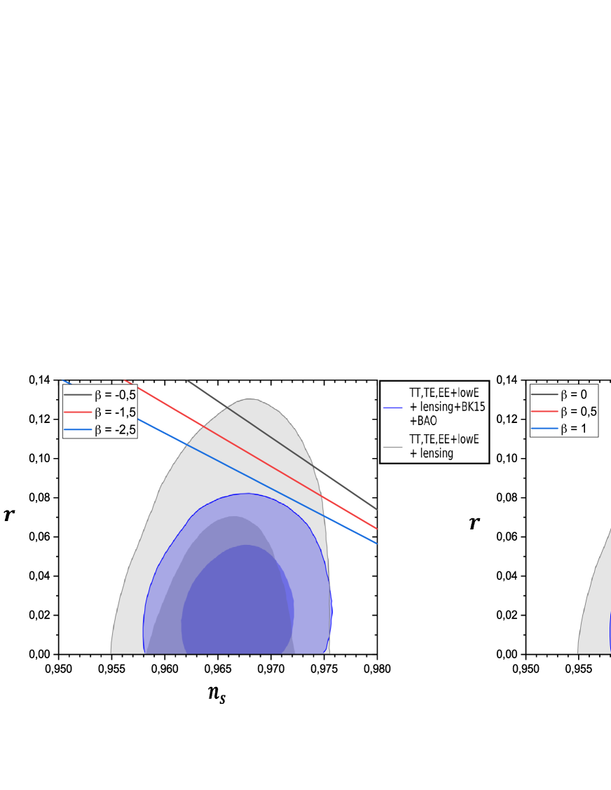
Figure 1: $r$ as a function of $n_{s}$ for a chaotic potential in modified symmetric teleparallel gravity, light and dark blue regions are constraints in combination with CMB lensing reconstruction and BAO from Planck data. on the right panel we choose three different values of $\beta$, the black line for $\beta=0$, the red line represents $\beta=0.5,$ and the blue line for $\beta=1$. While on the left one, We choose three different values of $\beta$, the black line for $\beta=-0.5$, the red line represents $\beta=-1.5,$ and the blue line for $\beta=-2.5$.

Fig. 1 show the decreasing behavior of the tensor-to-scalar ratio, $r$, with respect to the spectral index, $n_{s}$ for the chaotic potential in our chosen $f(Q,T)$ gravity model. The results show a good consistency for a specific range of the constant roll parameter $\beta$ with the latest observations from Planck data. Furthermore, the case with $\beta>0$ provides inconsistent results with Planck’s data. However, the constant roll parameter must be bounded as $\beta\leq 0$ in order to produce consistent observational parameters with recent results.

III.4 Hilltop inflation

Hilltop inflation is classified among small-field models. This potential naturally involves eternal inflation, that raises the question of initial conditions, which is a problem in most inflation models [116]. Hilltop potential is given by [117]

$$V\left(\phi\right)=M^{4}\left[1-\left(\frac{\phi}{\mu}\right)^{p}\right],$$ (59)

this model of inflation has two free parameters $M$ and ${\mu}$ plus the parameter $p$ that will be given specific values at the end of this section. The e-folds number during inflation using Eqs. (53) and (48) is given by

$$N\equiv\int_{\phi_{k}}^{\phi_{end}}\frac{H}{\dot{\phi}}d\phi\approx-\frac{(\beta+3)\left(\kappa+\sigma\right)}{3\alpha}\int_{\phi_{end}}^{\phi_{k}}\frac{V}{V^{\prime}}d\phi,$$ (60)

considering $\Phi=\phi/\mu$ and $p>2,$ the expression of inflationary e-folds number is given by

$$N=-\frac{\mu^{2}}{2p}\frac{(\beta+3)\left(\kappa+\sigma\right)}{3\alpha}\left[\Phi_{k}^{2}-\Phi_{end}^{2}+\frac{2}{p-2}\Phi_{k}^{2-p}-\frac{2}{p-2}\Phi_{end}^{2-p}\right],$$

here the subscripts $"_{k}"$ and $"_{end}"$ mean the time the pivot scale crossed outside the horizon and the end of inflation respectively. Since the slow roll parameters are defined by the value of the field at the horizon crossing $\Phi_{k},$ for this model $\epsilon$ and $\eta$ are calculated as follows

$$\epsilon = -\frac{9\alpha}{2(\beta+3)^{2}\left(\kappa+\sigma\right)}\frac{p^{2}}{\mu^{2}}\frac{\Phi_{k}^{2\left(p-1\right)}}{\left(1-\Phi_{k}^{p}\right)^{2}},$$ (61)

$$\eta = \frac{3\alpha}{(\beta+3)\left(\kappa+\sigma\right)}\frac{p\left(p-1\right)}{\mu^{2}}\frac{\Phi_{k}^{p-2}}{1-\Phi_{k}^{p}}.$$ (62)

Furthermore, we can compute the tensor-to-scalar ratio as a function of the inflationary e-folds $N$, the constant-roll parameter $\beta$ for $p>2$ in the following way,

$$r=\frac{4p}{(\beta+3)}\frac{1}{N}.$$ (63)

Taking into consideration Eq. (37), we can study the behavior of $r$ as a function of the spectral index $n_{s}$, $\beta$ and $p$ parameters using the first slow roll parameter $\epsilon$ given as

$$\epsilon = \frac{3p\left(1-n_{s}\right)}{18p-4\left(p-1\right)\left(\beta+3\right)},$$ (64)

$$\eta = \frac{2\left(p-1\right)\left(\beta+3\right)\left(1-n_{s}\right)}{-18p+4\left(p-1\right)\left(\beta+3\right)}.$$ (65)

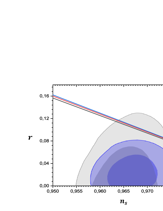
Figure 2: $r$ as a function of $n_{s}$ for the hilltop potential in modified symmetric teleparallel gravity, light and dark blue regions are constraints in combination with CMB lensing reconstruction and BAO from Planck data. We choose three different values of $p$, the black line for $p=3$, the red line represents $p=4$ and the blue line for $p=5$.

In Fig. 2, we consider the hilltop inflation, where the inflationary parameters are linked to $f(Q,T)$ gravity. It is apparent from the calculations that the constant roll parameter has negligible effects on the $\left(r,n_{s}\right)$ behavior, the plot shows that increasing the value of $p$ makes the decreasing function obtained from our model consistent with the latest observations provided by Planck’s results.

$\beta$	$p$	$N$	$r$
$-1.5$	$6$	$50$	$0.32$
$-1.1$	$5$	$55$	$0.19$
$-0.5$	$4$	$60$	$0.10$
$0.7$	$3$	$65$	$0.049$

Table 1: Testing the tensor-to-scalar ratio for different parameters for the hilltop inflation.

Based on the previously established equation Eq.(63), we provide an examination of the tensor-to-scalar ratio taking into account different inflation durations that varies from $50$ to $65$ e-folds. In addition to an increasing values of the constant roll $\beta$ parameter, the tensor-to-scalar ratio $r$ can be compatible with the observational bound for specific values of $p$ and $N$. Furthermore, the constant roll parameter and the inflationary e-folds provide compatible results only for higher values since they are inversely proportional to $r$.

Now as we construct a constant roll model for the $f(Q,T)$ gravity in the context of chaotic and hilltop inflation, we will study the evolution of primordial black holes that were supposed to occur just after the inflation period taking into account our $f(Q,T)$ gravity model.

IV Primordial black holes evolution in $f(Q,T)$ Gravity

IV.1 Rotating and non-rotating Primordial Black Holes

Primordial black holes abundance is determined by the primordial power spectrum. In fact, PBHs were formed as a result of amplification in the primordial power spectrum on small scales at the time when primordial inhomogeneities re-enter the Hubble horizon in a radiation-dominated Universe era. Some regions with a significant positive curvature which are considered equivalent to a closed Universe will collapse into a black hole [119]. At first, black holes were considered to be eternal and evolved with an increasing mass by absorbing more matter or even other stars and BHs. However, studying their quantum properties shows the possibility of emitting particles with a thermal spectrum related to BHs surface gravity [120, 35]. In this process of emitting particles, BHs lose mass and angular momentum with different properties depending on the specific characteristics of BHs. In this direction, we will discuss the thermal properties of evaporating PBHs for two cases namely the Schwarzschild and Kerr PBHs.

As an analogy to non-rotating Schwarzschild black holes, we consider a PBH with mass $M_{BH},$ the thermal spectrum of emitted particles from the evaporation process has the following expression [121]

$$T_{BH}=\frac{1}{8\pi GM_{BH}}\sim 1.06\left(\frac{10^{10}kg}{M_{BH}}\right)GeV,$$ (66)

Another option is that the evaporating BHs have some angular momentum, such spinning BHs, also known as Kerr BHs, might have originated with an initial spin or acquired their angular momenta by a variety of events, such as mergers [122, 123, 124]. A PBH temperature for the Kerr scenario can be modified due to their spinning and it’s given as [125]

$$T_{BH}=\frac{1}{4\pi GM_{BH}}\frac{\sqrt{1-a_{\ast}^{2}}}{1+\sqrt{1-a_{\ast}^{2}}},$$ (67)

where $a_{\ast}$ is a dimensionless parameter bounded by the interval $0\leq a_{\ast}\leq 1.$ The primary distinction between Kerr $\left(a_{\ast}\neq 0\right)$ and Schwarzschild $\left(a_{\ast}=0\right)$ BHs is that Kerr BHs are axially symmetric rather than spherically symmetric. When $a_{\ast}$ grows, the emission of particles with angular momentum spinning in the same direction as the BH is enhanced [126]. For the case $a_{\ast}=1$ a BH would have $T_{BH}=0,$ this is traditionally prohibited in any statistical system. Furthermore, its horizon would have vanished revealing a bare space-time singularity and contradicting the Cosmic Censorship Conjecture [126, 127, 128].

IV.2 Primordial Black Holes evolution

Since we are interested in studying the rate of mass loss from PBH, we recall the process which reduces the mass of the black hole due to Hawking evaporation which is defined by [129, 130]

$$\left(\frac{dM}{dt}\right)_{eva}=-\frac{\hbar c^{4}}{G^{2}}\frac{\alpha^{\prime}}{M_{BH}^{2}}.$$ (68)

where $G$ is Newton’s gravitational constant, $\hbar$ is the Planck constant, $c$ is light speed, $\alpha^{\prime}$ is the spin parameter of the emitting particles, and the black hole radius is given by $r_{BH}=2GM.$ After integration Eq. (68) we obtain the evolution of PBH mass as

$$M_{eva}=M_{i}\left(1-\frac{t}{t_{eva}}\right)^{\frac{1}{3}},$$ (69)

we can define the Hawking evaporation time scale $t_{eva}$ as

$$t_{eva}=\frac{G^{2}}{\hbar c^{4}}\frac{M_{i}^{3}}{3\alpha^{\prime}},$$ (70)

according to Ref. [131] fine-tuning the initial PBH masse $M_{i}$ along with the $\alpha^{\prime}$ parameter would be a good method to probe the early Universe. On the other hand, additional contributions suggest that the evaporation of PBHs would have interesting implications on the CMB and the standard cosmological nucleosynthesis scenario [132, 133].

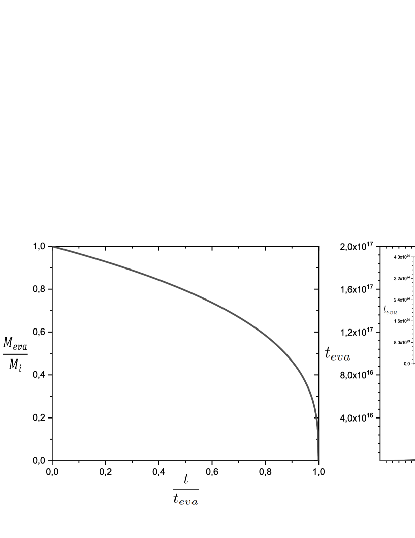
Figure 3: On the left, the evolution of the primordial black hole reduced the mass ratio to the initial mass $M_{eva}/M_{i}$ as functions of time ratio $t/t_{eva}$ is plotted. On the right, the evaporation time of primordial black holes as a function of the initial mass is presented, and the plot in the left corner shows the variation of $t_{eva}$ for higher values of $M_{i}.$  

In Fig. 3 we test the evolution of the primordial black holes evaporation and initial mass ratio $M_{eva}/M_{i}$ with respect to the ratio $t/t_{eva},$ and we plotted the variation of the evaporation time parameter $t_{eva}$ as functions of the initial mass of primordial black holes $M_{i}.$ Our results show that the evaporation mass can simply decrease as we move forward in time. However, one must study the effect of the initial primordial black holes masses on the time that must take in order to completely evaporate. In this direction, the second plot indicates that as we increase the initial mass of PBHs we need more time to achieve a complete evaporation process. In fact, an initial mass in the order of $M_{i}\gtrsim 10^{13}kg$ needs time more than the current age of our Universe to evaporate, as a result, we must consider lower bounds on PBHs initial mass for fine consistency with cosmic history.

The accretion of cosmic fluid surrounding the black hole will prolong the evaporation of the primordial black holes. Therefore, it is necessary to add a mass accretion rate which for a cosmic fluid with $\rho_{eff}$ and $p_{eff}$ will be given as

$$\left(\frac{dM}{dt}\right)_{accr}=\frac{16\pi G^{2}}{c^{5}}M^{2}\left(\rho_{eff}+p_{eff}\right),$$ (71)

which can be integrated to be in the final form [134]

$$M_{accr}=M_{i}\left(1-\frac{t}{t_{accr}}\right)^{-1},$$ (72)

where from Eqs. (42) and (43) the accretion time scale $t_{accr}$ is defined as

$$t_{accr}=\left[\frac{16\pi G^{2}}{c^{5}}M_{i}\left(\rho_{eff}+p_{eff}\right)\right]^{-1}.$$ (73)

Additionally, we can write the following equation

$$\rho_{eff}+p_{eff}=\frac{3}{\kappa}H^{2}\left(\frac{2\left(\sigma+\kappa\right)\left(1+\omega\right)}{2\kappa-\left(\omega-3\right)\sigma}\right)$$ (74)

Here, at a radiation-dominated era, and using the fact that the Hubble parameter is given by $H=\frac{\dot{a}}{a},$ we can simply choose $a(t)\propto t^{1/2}$ and finally obtain $H=1/\left(2t\right)^{2}$ to estimate the time at which the radiation surrounded primordial black-holes.

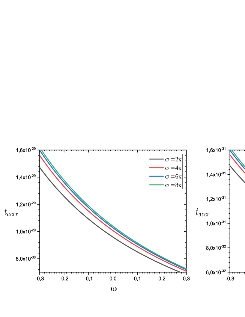
Figure 4: The accretion time $t_{accr}$ variation as a function of the equation of state in the interval $\omega\in\left[-0.3,0.3\right]$ considering different values of the $f(Q,T)$ gravity model parameter $\sigma$. The left panel provides the case for $M_{i}\propto 10^{12}kg,$ while the right shows the case of $M_{i}\propto 10^{14}kg$.

Fig. 4 illustrates the evolution of the accretion time as a function of a specific interval of the equation of state parameter. In our study, the accretion time is the moment at which primordial black holes started the accretion process, the variation of the accretion time shows to be minimally dependent on the choice of $\sigma$ parameter for our chosen $f(Q,T)$ gravity model. In fact, the behavior of accretion time increases for higher values of $\sigma$. Considering the fact that in order for inflation to initiate the EoS must be bounded by $\omega>-1/3.$ Moreover, $\omega$ evolves toward $1/3$ for inflation to be ended and the subsequent periods to take place [9, 135]. In Eq.(74) we choose a fixed value of time using the Hubble parameter which represents the time of PBHs formation, following the results of [129] which suggests that PBHs formed at $t\propto 10^{-23}s$, our results provide precise values of the time of accretion which decreases as we consider higher values of the EoS parameter. On the other hand, for lower initial PBHs masses, the accretion initiates sooner than in the case of higher $M_{i}$ values.

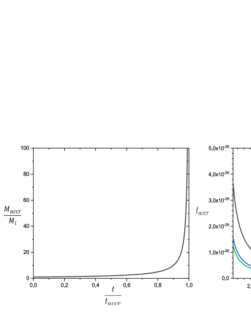
Figure 5: On the left panel, the evolution of the primordial black holes accretion mass ratio to the initial mass $M_{accr}/M_{i}$ as functions of the time ratio $t/t_{accr}$ is shown. On the right one, the accretion time of primordial black holes as a function of the initial mass is presented for specific values on the equation of state $\omega$ parameter.

In Fig. 5 we provide the variation of the primordial black holes accretion mass ratio to the initial mass $M_{accr}/M_{i}$ as a function of the ratio $t/t_{accr}.$ From this figure we conclude that when $t\longrightarrow t_{accr}$ the resulting primordial black hole mass due to the accretion process became in the order of $100M_{i}.$ On the other hand, accretion occurs faster when we consider more significant initial PBH masses for several values of $\omega$ parameter.

The total PBHs mass evolution may now be rewritten in the following form $M_{BH}=M_{eva}+M_{accr}$

$\sigma$	$\omega$	$t(s)$	$M_{i}(kg)$	$M_{BH}(kg)$	$T_{BH}(GeV)$
$1.5~{}\kappa$	$-0.3$	$10^{-15}$	$10^{6}$	$\sim 2\times 10^{6}$	$\sim 5.3\times 10^{3}$
$2~{}\kappa$	$-0.2$	$10^{-5}$	$10^{7}$	$\sim 1.9\times 10^{7}$	$\sim 5.3\times 10^{2}$
$2.5~{}\kappa$	$-0.1$	$10$	$10^{8}$	$\sim 1.9\times 10^{8}$	$\sim 53$
$3~{}\kappa$	$0$	$10^{5}$	$10^{9}$	$\sim 1.9\times 10^{9}$	$\sim 5.3$
$3.5~{}\kappa$	$0.1$	$10^{9}$	$10^{10}$	$\sim 1.9\times 10^{10}$	$\sim 53\times 10^{-2}$
$4~{}\kappa$	$0.2$	$10^{13}$	$10^{11}$	$\sim 1.9\times 10^{11}$	$\sim 53\times 10^{-3}$
$4.5~{}\kappa$	$0.3$	$10^{17}$	$10^{12}$	$\sim 1.9\times 10^{12}$	$\sim 53\times 10^{-4}$

Table 2: Testing the evolution of the total non-rotating PBHs masses and temperature in $f(Q,T)$ gravity.

$\sigma$	$\omega$	$t(s)$	$M_{i}(kg)$	$a_{\ast}$	$M_{BH}(kg)$	$T_{BH}(GeV)$
$1.5~{}\kappa$	$-0.3$	$10^{-15}$	$10^{6}$	$0.1$	$\sim 2\times 10^{6}$	$\sim 5.28\times 10^{3}$
$2~{}\kappa$	$-0.2$	$10^{-5}$	$10^{7}$	$0.3$	$\sim 1.9\times 10^{7}$	$\sim 5.17\times 10^{2}$
$2.5~{}\kappa$	$-0.1$	$10$	$10^{8}$	$0.5$	$\sim 1.9\times 10^{8}$	$\sim 49.1$
$3~{}\kappa$	$0$	$10^{5}$	$10^{9}$	$0.7$	$\sim 1.9\times 10^{9}$	$\sim 4.41$
$3.5~{}\kappa$	$0.1$	$10^{9}$	$10^{10}$	$0.9$	$\sim 1.9\times 10^{10}$	$\sim 32.1\times 10^{-2}$
$4~{}\kappa$	$0.2$	$10^{13}$	$10^{11}$	$0.96$	$\sim 1.9\times 10^{11}$	$\sim 23.1\times 10^{-3}$
$4.5~{}\kappa$	$0.3$	$10^{17}$	$10^{12}$	$0.99$	$\sim 1.9\times 10^{12}$	$\sim 13.1\times 10^{-4}$

Table 3: Testing the evolution of the total rotating PBHs masses and temperature in $f(Q,T)$ gravity.

From tables (2) and (3) we study the evolution of rotating and non-rotating PBHs masses and temperature as functions of different parameters. According to these results, we conclude that PBHs masses increase with higher initial masses $M_{i}$. On the other hand, PBHs temperature decreases as we move forward in time. Moreover, $T_{BH}$ is inversely proportional to PBHs masses which makes the temperature evolve from $TeV$ to $MeV$ taking into account masses in the order of $10^{12}kg.$ Finally, when we compare rotating and non-rotating black holes, we find that higher values of the parameter $a_{\ast}$ can simply lead to a lower temperature for the case of rotating PBHs.

V Concluding Remarks

Over the past few decades, numerous studies have been conducted to examine the early and late evolution of the Universe. The standard model of cosmology, based on general relativity (GR), has proven to be a reliable model for describing the dynamics of the Universe. However, there are still some unresolved issues, such as the flatness and horizon problems, that need to be addressed through further research on cosmological inflation. Additionally, while GR has been successful in predicting the behavior of the Universe, it is unable to fully explain the influence of dark sectors on its dynamics in a way that is consistent with observed data. As a result, it may be worthwhile to consider alternative models of gravity such $f(Q,T)$ model to address these challenges.

In this study, we examined constant-roll inflation in the context of $f(Q,T)$ gravity. To do this, we started by explaining the basic theory of cosmological inflation using the isotropic and homogeneous inflaton scalar field. We then assumed a flat FLRW spacetime and an equation of state $\omega,$ we provided a new technique for studying the constant-roll process and correlating the slow-roll equations to the constant-roll $\beta$ parameter based on the modified Friedmann equations obtained through $f(Q,T)$ gravity. Furthermore, we have calculated the inflationary observables, the spectral index $n_{s},$ and the tensor-to-scalar ratio $r$ for two cases of inflationary potentials, namely the chaotic and hiltop models. We showed that for each model, a bound on the constant-roll parameter is preferred. In the case of chaotic inflation, for a consistent value of $r$ and $n_{s},$ $\beta$ must be bounded as $\beta\leq 0.$ While for the Hiltop Inflation, several parameters are involved to reproduce compatible values of $r$ and $n_{s},$ for instance, we must consider the bounds $p\geq 3$, $N\geq 60,$ and $\beta\geq-0.5$ for a good index spectral and tensor-to-scalar ratio consistencies.

Finally, for the PBHs evolution in the context of $f(Q,T)$ gravity, we analyzed the accretion process and the evaporation through Hawking radiation. From the obtained results, we conclude that both the evaporated mass and the evaporation time are directly related to the initial mass $M_{i}$ that must be bounded as $M_{i}<10^{13}kg$ to be able to completely evaporate currently or much earlier in the cosmic time. For the accretion process, we can summarise that the accretion of matter and radiation are model dependent in the context of the $f(Q,T)$ gravity, which motivates us to explore the PBHs evolution in the framework of modified gravity. According to the results, if we supposed that PBHs formed at $t\propto 10^{-23}s$ the PBHs mass due to the accretion can reach $100M_{i}$ taking into account that for lower initial PBHs masses the accretion can occur faster. Lastly, we studied the PBHs evaporation taking into account the effect of several parameters, and concluded that the Hawking temperature can simply decrease for higher initial masses through the cosmic time for both rotating and non-rotating black holes.

References

- [1] A. A. Starobinsky, A New Type of Isotropic Cosmological Models Without Singularity, Phys. Lett. B 91 (1980), 99-102.
- [2] A. H. Guth, The Inflationary Universe: A Possible Solution to the Horizon and Flatness Problems, Phys. Rev. D 23 (1981), 347-356.
- [3] A. Albrecht and P. J. Steinhardt, Phys. Rev. Lett. 48 (1982), 1220-1223.
- [4] A. D. Linde, Cosmology for Grand Unified Theories with Radiatively Induced Symmetry Breaking, Phys. Lett. B 108 (1982), 389-393.
- [5] K. El Bourakadi, M. Bousder, Z. Sakhi, & M. Bennai, Preheating and reheating constraints in supersymmetric braneworld inflation. Eur. Phys. J. Plus, (2021), 136(8), 1-19.
- [6] S. Weinberg, Cosmology, Oxford Univ. Press (2008).
- [7] D. Baumann, Primordial Cosmology, PoS TASI2017 (2018), 009.
- [8] Y. Akrami et al. [Planck], Planck 2018 results. X. Constraints on inflation, Astron. Astrophys. 641 (2020), A10.
- [9] K. El Bourakadi, M. Ferricha-Alami, H. Filali, Z. Sakhi & M. Bennai,. Gravitational waves from preheating in Gauss–Bonnet inflation. Eur. Phys. J. C, (2021), 81(12), 1-8.
- [10] K. El Bourakadi, B. Asfour, Z. Sakhi, M. Bennai, & T. Ouali, Primordial black holes and gravitational waves in teleparallel Gravity. Eur. Phys. J. C, (2022), 82(9), 1-11.
- [11] K. El Bourakadi, Z. Sakhi, & M. Bennai, Preheating constraints in -attractor inflation and Gravitational Waves production. Int J Mod Phys A, (2022), [arXiv preprint arXiv:2209.09241].
- [12] M. Maggiore, Gravitational Waves. Vol. 2: Astrophysics and Cosmology, Oxford University Press, 2018.
- [13] P. A. R. Ade et al. [BICEP and Keck], Improved Constraints on Primordial Gravitational Waves using Planck, WMAP, and BICEP/Keck Observations through the 2018 Observing Season, Phys. Rev. Lett. 127 (2021) no.15, 151301.
- [14] L. M. Wang, V. F. Mukhanov and P. J. Steinhardt, On the problem of predicting inflationary perturbations, Phys. Lett. B 414 (1997), 18-27.
- [15] N. C. Tsamis and R. P. Woodard, Improved estimates of cosmological perturbations, Phys. Rev. D 69 (2004), 084005.
- [16] W. H. Kinney, Horizon crossing and inflation with large eta, Phys. Rev. D 72 (2005), 023515.
- [17] K. Dimopoulos, Ultra slow-roll inflation demystified, Phys. Lett. B 775 (2017), 262-265.
- [18] H. Motohashi and A. A. Starobinsky, constant-roll inflation, Eur. Phys. J. C 77 (2017) no.8, 538.
- [19] H. Motohashi and A. A. Starobinsky, Constant-roll inflation: confrontation with recent observational data, EPL 117 (2017) no.3, 39001.
- [20] S. Nojiri, S. D. Odintsov and V. K. Oikonomou, Constant-roll Inflation in Gravity, Class. Quant. Grav. 34 (2017) no.24, 245012.
- [21] F. Cicciarella, J. Mabillard and M. Pieroni, New perspectives on constant-roll inflation, JCAP 01 (2018), 024.
- [22] A. Ito and J. Soda, Anisotropic Constant-roll Inflation, Eur. Phys. J. C 78 (2018) no.1, 55.
- [23] Q. Gao, The observational constraint on constant-roll inflation, Sci. China Phys. Mech. Astron. 61 (2018) no.7, 070411.
- [24] M. H. Namjoo, H. Firouzjahi and M. Sasaki, Violation of non-Gaussianity consistency relation in a single field inflationary model, EPL 101 (2013) no.3, 39001.
- [25] Zel’dovich, Y. B., & Novikov, I. D. The hypothesis of cores retarded during expansion and the hot cosmological model. Soviet Astronomy, (1967), 10, 602.
- [26] Hawking, S., Gravitationally collapsed objects of very low mass. Mon. Not. R. Astron. Soc., (1971), 152(1), 75-78.
- [27] Carr, B. J., Gilbert, J. H., & Lidsey, J. E.. Black hole relics and inflation: Limits on blue perturbation spectra. Phys. Rev. D, (1994), 50(8), 4853.
- [28] Novikov, I.. Black holes. In Stellar Remnants (pp. 237-334), (1997), Springer, Berlin, Heidelberg.
- [29] Carr, B. J. . The Primordial black hole mass spectrum, (1975).
- [30] Khlopov, M. Y., & Polnarev, A. G.. Primordial black holes as a cosmological test of grand unification. Phys. Lett. B, (1980), 97(3-4), 383-387.
- [31] Chapline, G. F. Cosmological effects of primordial black holes. Nature, (1975). 253(5489), 251-252.
- [32] Bird, S., Cholis, I., Muñoz, J. B., Ali-Haïmoud, Y., Kamionkowski, M., Kovetz, E. D., … & Riess, A. G.. Did LIGO detect dark matter?. Phys. Rev. Lett., (2016), 116(20), 201301.
- [33] Sasaki, M., Suyama, T., Tanaka, T., & Yokoyama, S.. Primordial black hole scenario for the gravitational-wave event GW150914. (2016), Phys. Rev. Lett., 117(6), 061101.
- [34] Abbott, B., Jawahar, S., Lockerbie, N., & Tokmakov, K.. LIGO scientific collaboration and virgo collaboration (2016) gw150914: first results from the search for binary black hole coalescence with Advanced LIGO. Phys. Rev. D (12). issn 1550-2368. Phys. Rev. D, (2016), 93, 122003.
- [35] Hawking, S. W.. Particle creation by black holes. In Euclidean quantum gravity (1975), (pp. 167-188).
- [36] Alcock, C., Allsman, R. A., Alves, D. R., Axelrod, T. S., Becker, A. C., Bennett, D. P., … & MACHO Collaboration. (2001). MACHO Project Limits on Black Hole Dark Matter in the 1-30 Range. The Astrophys. J., 550(2), L169.
- [37] Tisserand, P., Le Guillou, L., Afonso, C., Albert, J. N., Andersen, J., Ansari, R., … & Vigroux, L.. Limits on the Macho Content of the Galactic Halo from the EROS-2 Survey of the Magellanic Clouds. Astron. Astrophys., (2007) 469(2), 387-404.
- [38] Quinn, D. P., Wilkinson, M. I., Irwin, M. J., Marshall, J., Koch, A., & Belokurov, V. . On the reported death of the MACHO era. Mon. Not. R. Astron. Soc. : Letters, (2009), 396(1), L11-L15.
- [39] Monroy-Rodríguez, M. A., & Allen, C. . The end of the MACHO era, revisited: new limits on MACHO masses from halo wide binaries. The Astrophys. J., (2014), 790(2), 159.
- [40] Carr, B. J.. Pregalactic black hole accretion and the thermal history of the universe. Mon. Not. R. Astron. Soc., (1981), 194(3), 639-668.
- [41] Ali-Haïmoud, Y., & Kamionkowski, M.. Cosmic microwave background limits on accreting primordial black holes. Phys. Rev. D, (2017), 95(4), 043534.
- [42] S. Weinberg, Gravitation and Cosmology: Principles and Applications of the General Theory of Relativity, John Wiley and Sons, (1972).
- [43] A. Unzicker and T. Case, Translation of Einstein’s attempt of a unified field theory with teleparallelism, [arXiv:physics/0503046 [physics]].
- [44] A. Einstein Riemannian Geometry with Maintaining the Notion of Distant Parallelism , Sitzungsber.Preuss.Akad.Wiss.Berlin (Math.Phys.) 217, (1928) 221.
- [45] A. Einstein, A theory of Gravitation, Math. Ann. 102, 685 (1930).
- [46] A. Einstein, A theory of Gravitation, Sitzungsber. Preuss. Akad. Wiss. Phys. Math. Kl. 24, 401 (1930).
- [47] C. Pellegrini and J. Plebanski, A theory of Gravitation, Math.-Fys. Skr. Dan. Vid. Selskab 2, 4 (1963).
- [48] C. Møller, On the crisis in the theory of gravitation and a possible solution, K. Dan.Vidensk. Selsk. Mat. Fys. Skr. 89, 13 (1978).
- [49] K. Hayashi and T. Nakano, Extended translation invariance and associated gauge fields, Prog. Theor. Phys., 38, 491 (1967).
- [50] K. Hayashi and T. Shirafuji, New general relativity, Phys. Rev. D 19, 3524 (1979).
- [51] J. G. Pereira, in Handbook of Spacetime, edited by A. Ashtekar and V. Petkov (Springer, 2014), pp. 212, 1302.6983.
- [52] V. C. de Andrade, L. C. T. Guillen, and J. G. Pereira, Phys. Rev. Lett. 84, 4533 (2000), gr-qc/0003100.
- [53] H. I. Arcos and J. G. Pereira, Int. J. Mod. Phys. D 13, 2193 (2004), gr-qc/0501017.
- [54] J. G. Pereira and Y. N. Obukhov, Universe 5, 139 (2019), 1906.06287.
- [55] Aldrovandi, R., Pereira, J. G., and Vu, K. H.Selected topics in teleparallel gravity. Braz. J. Phys., (2004). 34, 1374-1380.
- [56] G. R. Bengochea and R. Ferraro, Dark torsion as the cosmic speed-up, Phys. Rev. D 79 (2009), 124019.
- [57] E. V. Linder, Einstein’s Other Gravity and the Acceleration of the Universe, Phys. Rev. D 81 (2010), 127301 [erratum: Phys. Rev. D 82 (2010), 109902].
- [58] B. Li, T. P. Sotiriou and J. D. Barrow, Large-scale Structure in f(T) Gravity, Phys. Rev. D 83 (2011), 104017.
- [59] Y. F. Cai, S. Capozziello, M. De Laurentis and E. N. Saridakis, f(T) teleparallel gravity and cosmology, Rept. Prog. Phys. 79 (2016) no.10, 106901.
- [60] M. Hohmann, L. Järv and U. Ualikhanova, Covariant formulation of scalar-torsion gravity, Phys. Rev. D 97 (2018) no.10, 104011.
- [61] M. Gonzalez-Espinoza and G. Otalora, Generating primordial fluctuations from modified teleparallel gravity with local Lorentz-symmetry breaking, Phys. Lett. B 809 (2020), 135696.
- [62] T. Clifton, P. G. Ferreira, A. Padilla and C. Skordis, Modified Gravity and Cosmology, Phys. Rept. 513 (2012), 1-189.
- [63] S. Capozziello and M. De Laurentis, Extended Theories of Gravity, Phys. Rept. 509 (2011), 167-321.
- [64] A. De Felice and S. Tsujikawa, f(R) theories, Living Rev. Rel. 13 (2010), 3.
- [65] S. Nojiri and S. D. Odintsov, Unified cosmic history in modified gravity: from F(R) theory to Lorentz non-invariant models, Phys. Rept. 505 (2011), 59-144.
- [66] S. Nojiri and S. D. Odintsov, ‘Introduction to modified gravity and gravitational alternative for dark energy, eConf C0602061 (2006), 06.
- [67] E. R. Harrison, Scalar-tensor theory and general relativity, Phys. Rev. D 6 (1972), 2077-2079.
- [68] M. A. Skugoreva, E. N. Saridakis and A. V. Toporensky, Dynamical features of scalar-torsion theories, Phys. Rev. D 91 (2015), 044023.
- [69] M. Gonzalez-Espinoza, G. Otalora and J. Saavedra, Stability of scalar perturbations in scalar-torsion f(T,) gravity theories in the presence of a matter fluid, JCAP 10 (2021), 007.
- [70] G. Leon, A. Paliathanasis, E. N. Saridakis and S. Basilakos, Unified dark sectors in scalar-torsion theories of gravity, Phys. Rev. D 106 (2022) no.2, 024055.
- [71] L. K. Duchaniya, S. A. Kadam, J. Levi Said and B. Mishra, Dynamical systems analysis in gravity, [arXiv:2209.03414 [gr-qc]].
- [72] M. Gonzalez-Espinoza, R. Herrera, G. Otalora and J. Saavedra, Reconstructing inflation in scalar-torsion gravity, Eur. Phys. J. C 81 (2021) no.8, 731.
- [73] Y. Leyva, C. Leiva, G. Otalora and J. Saavedra, Inflation and primordial fluctuations in F(T) gravity’s rainbow, Phys. Rev. D 105 (2022) no.4, 043523.
- [74] M. Gonzalez-Espinoza and G. Otalora, Cosmological dynamics of dark energy in scalar-torsion gravity, Eur. Phys. J. C 81 (2021) no.5, 480.
- [75] J. M. Nester and H. J. Yo, Symmetric teleparallel general relativity, Chin. J. Phys. 37 (1999), 113.
- [76] J. Beltrán Jiménez, L. Heisenberg and T. Koivisto, Coincident General Relativity, Phys. Rev. D 98 (2018) no.4, 044048.
- [77] M. Adak and O. Sert, A Solution to symmetric teleparallel gravity, Turk. J. Phys. 29 (2005), 1-7.
- [78] M. Adak, The Symmetric teleparallel gravity, Turk. J. Phys. 30 (2006), 379-390.
- [79] M. Adak, Ö. Sert, M. Kalay and M. Sari, Symmetric Teleparallel Gravity: Some exact solutions and spinor couplings, Int. J. Mod. Phys. A 28 (2013), 1350167.
- [80] J. Beltran Jimenez and T. S. Koivisto, Spacetimes with vector distortion: Inflation from generalised Weyl geometry, Phys. Lett. B 756 (2016), 400-404.
- [81] M. Adak, Gauge Approach to The Symmetric Teleparallel Gravity, Int. J. Geom. Meth. Mod. Phys. 15 (2018) no.12, 1850198.
- [82] I. Soudi, G. Farrugia, V. Gakis, J. Levi Said and E. N. Saridakis, Polarization of gravitational waves in symmetric teleparallel theories of gravity and their modifications, Phys. Rev. D 100 (2019) no.4, 044008.
- [83] L. Järv, M. Rünkla, M. Saal and O. Vilson, Nonmetricity formulation of general relativity and its scalar-tensor extension, Phys. Rev. D 97 (2018) no.12, 124025.
- [84] T. Harko, T. S. Koivisto, F. S. N. Lobo, G. J. Olmo and D. Rubiera-Garcia, Coupling matter in modified gravity, Phys. Rev. D 98 (2018) no.8, 084043.
- [85] R. Lazkoz, F. S. N. Lobo, M. Ortiz-Baños and V. Salzano, Observational constraints of gravity, Phys. Rev. D 100 (2019) no.10, 104027.
- [86] J. Beltrán Jiménez, L. Heisenberg, T. S. Koivisto and S. Pekar, Cosmology in geometry, Phys. Rev. D 101 (2020) no.10, 103507.
- [87] J. Beltrán Jiménez, L. Heisenberg and T. S. Koivisto, The Geometrical Trinity of Gravity, Universe 5 (2019) no.7, 173.
- [88] Koussour, M., Shekh, S. H., & Bennai, M.Cosmic acceleration and energy conditions in symmetric teleparallel gravity. J. High Energy Phys. (2022).
- [89] Koussour, M., Shekh, S. H., & Bennai, M. Anisotropic nature of space–time in fQ gravity. Phys. Dark Universe, 101051, (2022).
- [90] Koussour, M., El Bourakadi, K., Shekh, S. H., Pacif, S. K. J., & Bennai, M.. Late-time acceleration in f (Q) gravity: Analysis and constraints in an anisotropic background. Ann. Phys., (2022), 445, 169092.
- [91] Koussour, M., Shekh, S. H., Hanin, A., Sakhi, Z., Bhoyer, S. R., & Bennai, M. Flat LRW Universe in logarithmic symmetric teleparallel gravity with observational constraints. (2022), arXiv preprint arXiv:2203.00413.
- [92] Koussour, M., Shekh, S. H., Govender, M., & Benna, M. (2022). Thermodynamical aspects of Bianchi type-I Universe in quadratic form of f (Q) gravity and observational constraints.J. High Energy Phys. (2022).
- [93] Xu, Y., Li, G., Harko, T., & Liang, S. D. (2019). gravity. Eur. Phys. J. C, 79(8), 1-19.
- [94] Arora, S., Pacif, S. K. J., Bhattacharjee, S., & Sahoo, P. K.. gravity models with observational constraints. Phys. Dark Universe, (2020), 30, 100664.
- [95] S. Arora and P. K. Sahoo, Energy conditions in gravity, Phys. Scripta 95 (2020) no.9, 095003.
- [96] S. Arora, J. R. L. Santos and P. K. Sahoo, Constraining gravity from energy conditions, Phys. Dark Univ. 31 (2021), 100790.
- [97] N. Godani and G. C. Samanta, FRW cosmology in f(Q,T) gravity, Int. J. Geom. Meth. Mod. Phys. 18 (2021) no.09, 2150134.
- [98] L. Pati, B. Mishra and S. K. Tripathy, Model parameters in the context of late time cosmic acceleration in gravity, Phys. Scripta 96 (2021) no.10, 105003
- [99] M. Shiravand, S. Fakhry and M. Farhoudi, Cosmological inflation in gravity, Phys. Dark Univ. 37 (2022), 101106.
- [100] C. Germani and T. Prokopec, On primordial black holes from an inflection point, Phys. Dark Univ. 18 (2017), 6-10.
- [101] H. Di and Y. Gong, Primordial black holes and second order gravitational waves from ultra-slow-roll inflation, JCAP 07 (2018), 007.
- [102] T. Ortin, Gravity and Strings, Cambridge Monographs on Mathematical Physics (Cambridge University Press (2015)).
- [103] Bajardi, F., Vernieri, D., & Capozziello, S.. Bouncing cosmology in f (Q) symmetric teleparallel gravity. Eur. Phys. J. Plus, (2020), 135(11), 1-14.
- [104] Shiravand, M., Fakhry, S., & Farhoudi, M.. Cosmological Inflation in Gravity. (2022), arXiv preprint arXiv:2204.00906.
- [105] Liddle, A. R., Parsons, P., & Barrow, J. D.. Formalizing the slow-roll approximation in inflation. Phys. Rev. D, (1994) 50(12), 7222.
- [106] Odintsov, S. D., Oikonomou, V. K., & Sebastiani, L.. Unification of constant-roll inflation and dark energy with logarithmic R2-corrected and exponential F(R) gravity. Nucl. Phys. B., (2017), 923, 608-632.
- [107] Liddle, A. R.. An introduction to cosmological inflation. High energy physics and cosmology, 260, (1998).
- [108] Baumann, D.. TASI lectures on inflation. arXiv preprint arXiv:0907.5424, (2009).
- [109] Shokri, M., Sadeghi, J., & Gashti, S. N.. Constant-roll inflation from a Lorentzian function. arXiv preprint arXiv:2107.04756, (2021).
- [110] Planck collaboration, Planck 2018 results. VI. Cosmological parameters, Astron. Astrophys. 641, A6 (2020) [1807.06209].
- [111] P. A. R. Ade et al. (Planck Collaboration), Astron. Astrophys. 594, A20 (2016).
- [112] Motohashi, H., Mukohyama, S., & Oliosi, M.. Constant roll and primordial black holes. JCAP, 2020(03), 002.
- [113] H. Motohashi, A. A. Starobinsky, and J. Yokoyama, J. Cosmol. Astropart. Phys. 09 (2015) 018.
- [114] J. Martin, H. Motohashi, and T. Suyama, Phys. Rev. D 87, 023514 (2013).
- [115] M. H. Namjoo, H. Firouzjahi, and M. Sasaki, Europhys. Lett. 101, 39001 (2013).
- [116] Boubekeur, L., & Lyth, D. H., Hilltop inflation. JCAP, 2005(07), 010.
- [117] Linde, A. D. A new inflationary universe scenario: a possible solution of the horizon, flatness, homogeneity, isotropy and primordial monopole problems. Phys. Lett. B, (1982), 108(6), 389-393.
- [118] Cook, J. L., Dimastrogiovanni, E., Easson, D. A., & Krauss, L. M., Reheating predictions in single field inflation. JCAP, 2015(04), 047.
- [119] Zhou, Z., Jiang, J., Cai, Y. F., Sasaki, M., & Pi, S., Primordial black holes and gravitational waves from resonant amplification during inflation. Phys. Rev. D, (2020), 102(10), 103527.
- [120] Hawking, S. W., Black hole explosions?. Nature, (1974), 248(5443), 30-31.
- [121] Coogan, A., Morrison, L., & Profumo, S., Direct detection of Hawking radiation from asteroid-mass primordial black holes. Phys. Rev. Lett., (2021), 126(17), 171101.
- [122] Buonanno, A., Kidder, L. E., & Lehner, L.. Estimating the final spin of a binary black hole coalescence. Phys. Rev. D, (2008), 77(2), 026004.
- [123] Kesden, M.. Can binary mergers produce maximally spinning black holes?. Phys. Rev. D, (2008), 78(8), 084030.
- [124] Tichy, W., & Marronetti, P.. Final mass and spin of black-hole mergers. Phys. Rev. D, (2008), 78(8), 081501.
- [125] Cheek, A., Heurtier, L., Perez-Gonzalez, Y. F., & Turner, J. Primordial black hole evaporation and dark matter production. I. Solely Hawking radiation. Phys. Rev. D, (2022), 105(1), 015022.
- [126] Arbey, A., Auffinger, J., & Silk, J.. Evolution of primordial black hole spin due to Hawking radiation. Mon. Not. R. Astron. Soc., (2020) 494(1), 1257-1262.
- [127] Belgiorno, F., & Martellini, M.. Black holes and the third law of thermodynamics. Int. J. Mod. Phys. D, (2004), 13(04), 739-770.
- [128] Lehmann, B. V., Johnson, C., Profumo, S., & Schwemberger, T., Direct detection of primordial black hole relics as dark matter. JCAP, 2019(10), 046.
- [129] Nayak, B., & Singh, L. P.. Accretion, primordial black holes and standard cosmology. Pramana, (2011), 76(1), 173-181.
- [130] Page, D. N. (1976). Particle emission rates from a black hole. II. Massless particles from a rotating hole. Phys. Rev. D, 14(12), 3260.
- [131] Jamil, M., & Qadir, A. Primordial black holes in phantom cosmology. General Relativity and Gravitation, (2011), 43(4), 1069-1082.
- [132] Acharya, S. K., & Khatri, R. (2020). CMB and BBN constraints on evaporating primordial black holes revisited. JCAP, 2020(06), 018.
- [133] Novikov, I. D., Polnarev, A. G., Starobinskii, A. A., & Zeldovich, I. B.. Primordial black holes. Astron. Astrophys., (1979), 80, 104-109.
- [134] Babichev, E., Dokuchaev, V., & Eroshenko, Y., Black hole mass decreasing due to phantom energy accretion. Phys. Rev. Lett., (2004), 93(2), 021102.
- [135] K.D. Lozanov, M.A. Amin, Equation of state and duration to radi ation domination after inflation. Phys. Rev. Lett. 119.6, 061301 (2017).