Power Corrections to Energy Flow Correlations from Large Spin Perturbation

Abstract

Dynamics of high energy scattering in Quantum Chromodynamics (QCD) are primarily probed through detector energy flow correlations. One important example is the Energy-Energy Correlator (EEC), whose back-to-back limit probes correlations of QCD on the lightcone and can be described by a transverse-momentum dependent factorization formula in the leading power approximation. In this work, we develop a systematic method to go beyond this approximation. We identify the origin of logarithmically enhanced contributions in the back-to-back limit as the exchange of operators with low twists and large spins in the local operator product expansion. Using techniques from the conformal bootstrap, the large logarithms beyond leading power can be resummed to all orders in the perturbative coupling. As an illustration of this method, we perform an all-order resummation of the leading and next-to-leading logarithms beyond the leading power in ${\cal N}=4$ Super Yang-Mills theory.

I Introduction

Distributions of energy flows in high energy scattering in Quantum Chromodynamics (QCD) encode unique information of the Lorentizian dynamics of quantum gauge theory, which is otherwise hard to extract. A famous example is the formation of jets, which are collimated sprays of hadrons that manifest the underlying structure of of quark and gluon scattering Hanson et al. (1975); Sterman and Weinberg (1977). From the early days of QCD, global energy flow distributions have been characterized using infrared and collinear safe shape functions Bjorken and Brodsky (1970); Ellis et al. (1976); Georgi and Machacek (1977); Farhi (1977); Parisi (1978); Donoghue et al. (1979); Rakow and Webber (1981); Berger et al. (2003); Stewart et al. (2010). Alternatively, it can also be studied using statistical correlation of final-state energy flows, of which the simplest one is the two-point Energy-Energy Correlator (EEC) Basham et al. (1978a, b, 1979a, 1979b). In fact, the two different approaches for analyzing energy flow distributions are closely related by an integral transformation Belitsky et al. (2001); Sterman (2004); Komiske et al. (2018); Chen et al. (2020).

In the $e^{+}e^{-}$ scattering, EEC can be written as the Fourier transformation of the correlation function of energy flow operators

$$\text{EEC}(y)=\frac{8\pi^{2}}{q^{2}\sigma_{0}}\!\int\!d^{4}x\,e^{iq\cdot x_{13}}\langle J^{\mu}(x_{1}){\cal E}(n_{2}){\cal E}(n_{4})J_{\mu}^{\dagger}(x_{3})\rangle\,,$$ (1)

where $n_{2}=(1,\vec{n}_{2})$ and $n_{4}=(1,\vec{n}_{4})$ specify the directions of the detected energy flow in the collider, $y=1-\frac{(n_{2}\cdot n_{4})q^{2}}{2(n_{2}\cdot q)(n_{4}\cdot q)}=(1+\cos\theta)/2$, $q^{2}>0$ is a timelike momentum, $J^{\mu}$ is the electromagnetic current, and the energy flow operator is defined as a detector time integral of the energy-momentum tensor Sveshnikov and Tkachov (1996); Tkachov (1997); Korchemsky and Sterman (1999); Bauer et al. (2008); Hofman and Maldacena (2008); Belitsky et al. (2014a, b); Kravchuk and Simmons-Duffin (2018)

$$\mathcal{E}(n_{i})=\int\displaylimits_{-\infty}^{\infty}\frac{d\,n_{i}\!\cdot\!x_{i}}{16}\lim_{\bar{n}_{i}\!\cdot\!x_{i}\to\infty}(\bar{n}_{i}\cdot x_{i})^{2}T_{\mu\nu}(x_{i})\bar{n}_{i}^{\mu}\bar{n}_{i}^{\nu}\,.$$ (2)

Experimental studies of EEC have a long history Abe et al. (1995); Adrian et al. (1992); Acton et al. (1992); Adachi et al. (1989); Braunschweig et al. (1987); Bartel et al. (1984); Fernandez et al. (1985); Wood et al. (1988); Behrend et al. (1982); Berger et al. (1985). They have been used to provide precision extraction of strong coupling constant de Florian and Grazzini (2005); Kardos et al. (2018).

Intuitively, when two narrow jets are produced in $e^{+}e^{-}$, they tend to be back-to-back due to momentum conservation, reflecting the underlying $q\bar{q}$ production. This leads to a peak for EEC as $y\to 0$, known as the Sudakov peak. In perturbation theory, it is manifested as large logarithmic corrections,

$$\text{EEC}(y)\sim\sum_{n=1}^{\infty}\sum_{m=0}^{2n-1}\alpha_{s}^{n}\left(c_{n,m}\frac{\log^{m}y}{y}+d_{n,m}\log^{m}y\right)\,,$$ (3)

where we have only shown the Leading Power (LP, $\sim y^{-1}$) and the Next-to-Leading Power (NLP, $\sim y^{0}$) corrections for simplicity. The leading power series of EEC resembles the perturbative structure of vector boson production at small $p_{T}$ and exhibits lightcone divergences. It can be resummed to all orders in the perturbative coupling by solving a 2d renormalization group equation in virtuality and rapidity Collins and Soper (1981); Moult and Zhu (2018). Using the recently available 4-loop rapidity anomalous dimension Moult et al. (2022); Duhr et al. (2022), its perturbative resummation has been performed to N⁴LL accuracy Duhr et al. (2022). However, power corrections to EEC, and in general to event shape functions and transverse momentum dependent observables, are much less understood, both perturbatively and non-perturbatively. Recently there have been significant developments towards a more satisfying picture of power corrections for various observables, see e.g. Pirjol and Stewart (2003); Beneke et al. (2002); Bonocore et al. (2015a, b); Moult et al. (2017a); Boughezal et al. (2017); Feige et al. (2017); Del Duca et al. (2017); Moult et al. (2017b, 2018a); Goerke and Inglis-Whalen (2018); Beneke et al. (2018a); Moult et al. (2018b); Ebert et al. (2018); Beneke et al. (2018b); Boughezal et al. (2018); Ebert et al. (2019); Moult et al. (2019); van Beekveld et al. (2020); Bahjat-Abbas et al. (2019); Bacchetta et al. (2019); Cieri et al. (2019); Buonocore et al. (2020); Moult et al. (2020a); Beneke et al. (2020a); Moult et al. (2020b); Liu and Neubert (2020); Ebert et al. (2021); Beneke et al. (2020b); Luisoni et al. (2021); Inglis-Whalen et al. (2021a, b); Liu et al. (2021a, b); van Beekveld et al. (2021a, b); Salam and Slade (2021); Caola et al. (2022); Ebert et al. (2022); Vladimirov et al. (2022); Buonocore et al. (2022); Camarda et al. (2022); Luke et al. (2022); Liu et al. (2022); Gamberg et al. (2022). Yet the status is still far from that of leading power terms.

In this work we initiate a study of power corrections to EEC by exploiting conformal symmetry and techniques from the analytic conformal bootstrap Rychkov (2016); Simmons-Duffin (2017); Poland et al. (2019); Bissi et al. (2022). Building upon an important observation by Korchemsky Korchemsky (2020), we connect the logarithmically enhanced terms in power corrections ($m>0$ in (3)) with the expansion of correlators around the double lightcone limit, which is controlled by the twist expansion and the large spin expansion. Using twist conformal blocks Alday (2017), tails from large spins can be systematically resummed. Further simplifications come from crossing symmetry, which relates the twist corrections with large spin corrections. Using this method, we explicitly carry out a calculation in ${\cal N}=4$ super Yang-Mills (SYM) theory, and achieve the first Leading and Next-to-Leading Logarithmic resummation at the subleading power.

II Back-to-back v.s. double lightcone

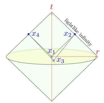
Figure 1: Penrose diagram for the double lightcone limit of the local correlator.

As is clear from (1), EEC is related to the local Wightman correlator $\langle\Omega|J(x_{1})T(x_{2})T(x_{4})J(x_{3})|\Omega\rangle$ by detector time integrals and a Fourier transform Belitsky et al. (2014a, b). It is useful to understand which region of the local correlator corresponds to the $y\to 0$ limit of EEC. Let us backtrack the dominant contribution by first undoing the Fourier transformation. We can apply a Lorentz transformation to make the two detectors exactly back-to-back: $n_{4}^{\mu}\to\bar{n}_{2}^{\mu}=(1,-\vec{n}_{2})$. At the same time, the momentum $q^{\mu}$ gains a small transverse component $\vec{q}^{\perp}$, which is schematically related to $y$ as $|\vec{q}^{\perp}|^{2}/q^{2}\sim y$. In position space, this corresponds to the region where $|(n_{2}\cdot x_{13})(\bar{n}_{2}\cdot x_{13})/x_{13}^{2}|\sim y$. Since $\mathcal{E}(n_{2})\mathcal{E}(\bar{n}_{2})$ is invariant under the boost along $\vec{n}_{2}$, we have an extra degree of freedom to choose a frame such that $n_{2}\cdot x_{13},\bar{n}_{2}\cdot x_{13}\sim\sqrt{y}|x_{13}|$. In such a frame, the lightcone singularities of $1$ and $3$ are very close on the path of detector time integrals of $2$ and $4$. Therefore, we expect the dominant contribution to come from the region where $2$ and $4$ are near the pinch of lightcone singularities: $x_{12}^{2},x_{23}^{2},x_{34}^{2},x_{14}^{2}\ll x_{13}^{2},x_{24}^{2}$, which is the null square configuration Alday et al. (2011). Instead, we can also choose the frame that $n_{2}\cdot x_{13}\sim y|x_{13}|,\bar{n}_{2}\cdot x_{13}\sim|x_{13}|$. Then the leading $y\to 0$ dependence comes from 2 being near the lightcone limit of both $1$ and $3$, which is called the double lightcone limit. In this work we delineate this correspondence and systematically go beyond the leading power results in Korchemsky (2020).

It is well known that the lightcone limit is controlled by twist expansion Ferrara et al. (1971, 1972); Christ et al. (1972); Muta (1998). The most singular behavior in the $1,2$-channel as $x_{12}^{2}\to 0$ is produced by operators with the lowest twist $\tau=\Delta-\ell$. However, any single operator in the $1,2$-channel cannot generate the lightcone singularity in the crossed channel with $x_{13}^{2}\to 0$. The $x_{13}^{2}\to 0$ singularity can only be produced by an infinite sum of operators with different spins at a given twist. Therefore, the double lightcone limit, or relatedly the back-to-back limit of EEC, is determined by the large spin asymptotics of low-twist operators.

To be specific, we now consider EEC in ${\cal N}=4$ SYM. Comments for QCD will be given at the end. We consider the correlator of scalar operators belonging to the stress tensor supermultiplet

$$\langle\mathcal{O}(x_{1})\mathcal{O}(x_{2})\mathcal{O}(x_{3})\mathcal{O}(x_{4})\rangle_{\rm dyn}=\frac{1}{(2\pi)^{4}}\frac{x_{13}^{4}x_{24}^{4}}{(x_{12}^{6}x_{34}^{2})^{6}}\mathcal{F}(u,v)\,.$$ (4)

Here we have only kept the dynamical part and subtracted the contribution of protected operators which are not perturbatively corrected, see Supplemental Material for details. Conformal symmetry ensures that $\mathcal{F}$ is a function of the conformal cross ratios

$$u=\frac{x_{12}^{2}x_{34}^{2}}{x_{13}^{2}x_{24}^{2}}=z\bar{z}\;,\quad v=\frac{x_{23}^{2}x_{14}^{2}}{x_{13}^{2}x_{24}^{2}}=(1-z)(1-\bar{z})\;.$$ (5)

Expanded in the small coupling $a=\frac{g^{2}N_{c}}{4\pi^{2}}$, $\mathcal{F}(u,v)$ reads

$$\mathcal{F}(u,v)=\sum_{n=0}^{\infty}a^{n}\mathcal{F}^{(n)}(u,v)=\mathcal{F}^{(0)}(u,v)+\frac{u^{3}}{v}\Phi(u,v)\,,$$ (6)

The new function $\Phi(u,v)=\sum_{n\geq 1}a^{n}\Phi^{(n)}(u,v)$ packages all the coupling dependent information and is crossing symmetric, i.e., $\Phi(u,v)=\Phi(v,u)$. It has been calculated to three loops in Eden et al. (2012); Drummond et al. (2013). The correlator admits the following superconformal block decomposition Dolan and Osborn (2002); Beem et al. (2017):

$$\mathcal{F}(u,v)=\sum_{\Delta}\sum_{\text{even }\ell}a_{\tau,\ell}G_{\Delta+4,\ell}(u,v)\,.$$ (7)

Here the sums are over all superconformal primary operators with dimension $\Delta$, spin $\ell$ and OPE coefficient $a_{\tau,\ell}$. The use of $\tau$ in the label foreshadows the twist expansion later. The 4d bosonic conformal blocks are given by Dolan and Osborn (2001)

$$G_{\Delta,\ell}(u,v)=\frac{z\bar{z}}{\bar{z}-z}\left[k_{\Delta-\ell-2}(z)k_{\Delta+\ell}(\bar{z})-(z\leftrightarrow\bar{z})\right]\,,$$ (8)

where $k_{\beta}(x)=x^{\beta/2}{}_{2}F_{1}(\frac{\beta}{2},\frac{\beta}{2},\beta;x)$. They are eigenfunctions of the quadratic Casimir operator

$$\mathcal{D}_{2}=z^{2}((1-z)\partial_{z}^{2}-\partial_{z})+\frac{(d-2)z\bar{z}}{z-\bar{z}}(1-z)\partial_{z}+(z\leftrightarrow\bar{z})$$ (9)

with eigenvalues $\frac{1}{2}\left(\Delta(\Delta-4)+\ell(\ell+2)\right)$ Dolan and Osborn (2004). Superconformal symmetry causes a shift $\Delta\to\Delta+4$ in the expansion (7), and we denote $\mathbf{G}_{\tau,\ell}(z,\bar{z})=G_{\Delta+4,\ell}(u,v)$ for convenience. Perturbative corrections, via conformal block decomposition, are encoded in the expansions of twists and OPE coefficients

$$\tau=\tau_{0}+\sum_{n=1}^{\infty}a^{n}\gamma^{(n)}_{\tau_{0},\ell}\,,\quad a_{\tau,\ell}=\sum_{n=0}^{\infty}a^{n}a^{(n)}_{\tau_{0},\ell}\,,$$ (10)

where $\tau_{0}$ is the classical twist and $\sum_{n\geq 1}a^{n}\gamma^{(n)}_{\tau_{0},\ell}=\gamma_{\tau,\ell}$ is the anomalous dimension. The anomalous dimensions enter via the expansion for conformal blocks: $\mathbf{G}_{\tau,\ell}=\sum_{n=0}^{\infty}\frac{1}{n!}\gamma_{\tau,\ell}^{n}\partial_{\tau_{0}}^{n}\mathbf{G}_{\tau_{0},\ell}$. Note that $\partial_{\tau_{0}}^{n}\mathbf{G}_{\tau_{0},\ell}$ contains at most $\log^{n}u$ in the small $u$ limit.

The double lightcone limit corresponds to $u,v\to 0$, or equivalently, $z\to 0,\,\bar{z}\to 1$. Each conformal block in this limit is controlled by the twist $G_{\Delta,\ell}(z,\bar{z})\sim z^{\tau/2}\log(1-\bar{z})$. The presence of logarithms partially demonstrates the effect of summing over infinitely many spinning operators because each conformal block contains infinitely many descendants in a given conformal family. However, we will encounter more divergent pieces than a single logarithm, which require the large spin contribution from infinitely many primary operators. Examples include power divergences $(1-\bar{z})^{m<0}$ and powers of logarithms $[\log(1-\bar{z})]^{k\geq 2}$ . The latter arises from $\log^{k}u$ of $\partial_{\tau_{0}}^{k}\mathbf{G}_{\tau_{0},\ell}$ in small $u$ under crossing. In the following, we refer to these as enhanced divergences. To lighten the notations, we will denote the logarithms as $\log(x)=L_{x}$ from now on.

We also point out that crossing symmetry will play an important role in our computation of the power corrections. As we will see, the $u$, $v$ power corrections to $\Phi(u,v)$ contribute equally to the $y$ power corrections in EEC. In particular, EEC at NLP corresponds to order $u^{0}v^{1}$ and $u^{1}v^{0}$ in $\Phi(u,v)$. The former only requires twist-2 data to subleading order in the large spin limit ($\mathcal{O}(\ell^{-2})$), while the latter contains twist-4 contributions. Crossing symmetry equates these two contributions and therefore avoids the necessity of inputting the twist-4 information.

Table 1: CFT data needed at different orders

	Power Corrections		Perturbative Corrections
	twist	large spin	LL	NLL
LP	2	$\mathcal{O}(\ell^{0})$	$a_{2,\ell}^{(0)}\,,\gamma_{2,\ell}^{(1)}$	$a_{2,\ell}^{(1)}\,,\gamma_{2,\ell}^{(2)}$
NLP	2	$\mathcal{O}(\ell^{-2})$	$a_{2,\ell}^{(0)}\,,\gamma_{2,\ell}^{(1)}$	$a_{2,\ell}^{(1)}\,,\gamma_{2,\ell}^{(2)}$
	4	$\mathcal{O}(\ell^{0})$	$a_{4,\ell}^{(0)}\,,\gamma_{4,\ell}^{(1)}$	$a_{4,\ell}^{(1)}\,,\gamma_{4,\ell}^{(2)}$

Before going into the technical details, we provide a brief overview for the next two sections. We will first use techniques from large spin perturbation theory to extract the enhanced divergences in $v$ at twist-2 up to NLP. That is, we will obtain $\Phi(u,v)=p_{0}(L_{u},L_{v})+p_{1}(L_{u},L_{v})v+\cdots$, in which $p_{0}$, $p_{1}$ are polynomials in $L_{u}$, $L_{v}$ at each perturbative order. Crossing symmetry then fixes the NLP contribution in $u$ to be $\Phi(u,v)=p_{0}(L_{u},L_{v})+p_{1}(L_{u},L_{v})v+p_{1}(L_{v},L_{u})u\cdots$. The relevant data is listed in Table 1, but only the first two rows are needed thanks to crossing symmetry. Finally, we map the small $u$, $v$ expansion of $\Phi(u,v)$ to the back-to-back limit of $\mathrm{EEC}(y)$. The rules at LP and NLP are given in Table 2 and are valid to NLL accuracy. We will explain these points in more detail in the rest of the paper.

Table 2: Logarithms Map at LP and NLP

	$\Phi(u,v)$	$4y(1-y)^{2}\times\mathrm{EEC}(y)$
LP	$L_{u}^{m}L_{v}^{m}$	$2(m+n)L^{m+n-1}_{y/(1-y)}$
NLP	$uL_{u}^{m}L_{v}^{n}$	$\frac{2m(1-m)}{m+n-1}\frac{y}{1-y}L^{m+n-1}_{y/(1-y)}$
	$vL_{u}^{m}L_{v}^{n}$	$\frac{2n(1-n)}{m+n-1}\frac{y}{1-y}L^{m+n-1}_{y/(1-y)}$

III Large spin analysis

The enhanced divergences can be systematically handled by using the Large Spin Perturbation Theory Alday (2017), which culminates an array of earlier works in the large spin sector Alday and Maldacena (2007); Fitzpatrick et al. (2013); Komargodski and Zhiboedov (2013); Alday and Bissi (2013); Alday et al. (2015); Alday and Zhiboedov (2016, 2017). The starting point is the free theory limit where the twists are degenerate. The correlators can be written as a sum over the twists

$$\mathcal{F}^{(0)}(z,\bar{z})=\sum_{\tau_{0}=2,4,\ldots}H_{\tau_{0}}(z,\bar{z})\;,$$ (11)

where each $H_{\tau_{0}}(z,\bar{z})$ sums over spins

$$H_{\tau_{0}}(z,\bar{z})=\sum_{\ell=0}^{\infty}\langle a_{\tau_{0},\ell}^{(0)}\rangle\mathbf{G}_{\tau_{0},\ell}(z,\bar{z})\;,$$ (12)

and is known as a twist conformal block (TCB). When the interaction is turned on, the twist degeneracies are lifted and the OPE coefficients are corrected. In general, we find that the expansion consists of sums of the form

$$\sum_{\ell=0}^{\infty}\langle a_{\tau_{0},\ell}^{(0)}\rangle\kappa_{\tau_{0}}(\ell)\mathbf{G}_{\tau_{0},\ell}(z,\bar{z})\;,$$ (13)

where the quantities $\kappa_{\tau_{0}}(\ell)$ admit expansions around large conformal spins $J^{2}_{\tau,\ell}=(\ell+\frac{\tau}{2})(\ell+\frac{\tau}{2}-1)$ with the following schematic form

$$\kappa_{\tau_{0}}(\ell)=\sum_{m=0}^{\infty}\sum_{i=0}^{N}\frac{K_{m,i}}{J_{\tilde{\tau}_{0},\ell}^{2m}}\log^{i}J_{\tilde{\tau}_{0},\ell}^{2}\;.$$ (14)

Here we introduce shifted twists $\tilde{\tau}_{0}=\tau_{0}+4$ to take into account the dimension shift in the decomposition (7). An interesting feature, as we will see in explicit calculations, is that only even negative powers appear in the expansion. This is closely related to the reciprocity relation Dokshitzer et al. (2006); Basso and Korchemsky (2007), which has been explicitly verified in QCD to three loops Chen et al. (2021). Consequently, the correlator should now be expanded in terms of a more general class of TCBs

$$H_{\tau_{0}}^{(m,i)}(z,\bar{z})=\sum_{\ell}a^{(0)}_{\tau_{0},\ell}\frac{\log^{i}J^{2}_{\tilde{\tau}_{0},\ell}}{J_{\tilde{\tau}_{0},\ell}^{2m}}\mathbf{G}_{\tau_{0},\ell}(z,\bar{z})\;.$$ (15)

Note that conformal blocks satisfy the Casimir equation

$$\mathcal{C}_{\tilde{\tau}_{0}}\mathbf{G}_{\tau_{0},\ell}(z,\bar{z})=J_{\tilde{\tau}_{0},\ell}^{2}\mathbf{G}_{\tau_{0},\ell}(z,\bar{z})\;,$$ (16)

where $\mathcal{C}_{\tau}=\mathcal{D}_{2}+\frac{1}{4}\tau(2d-\tau-2)$ is the shifted conformal Casimir. It follows that TCBs obey the following recursion relations

$$H_{\tau_{0}}^{(m,i)}(z,\bar{z})=\mathcal{C}_{\tilde{\tau}_{0}}H_{\tau_{0}}^{(m+1,i)}(z,\bar{z})\;.$$ (17)

The full TCBs are in general difficult to compute. However, we will only need them in the small $v$ limit where computations become manageable. The TCBs in 4D take a factorized form

$$H_{\tau_{0}}^{(m,i)}(z,\bar{z})=\frac{z\,k_{\tilde{\tau}_{0}-2}(z)}{\bar{z}-z}\bar{H}_{\tau_{0}}^{(m,i)}(\bar{z})\;,$$ (18)

where we have dropped the regular part when $\bar{z}\to 1$. Moreover, the recursion relation (17) becomes

$$\bar{H}_{\tau_{0}}^{(m,i)}(\bar{z})=\bar{D}\bar{H}_{\tau_{0}}^{(m+1,i)}(\bar{z})\;,$$ (19)

where

$$\bar{D}=\bar{z}^{2}(1-\bar{z})\frac{d^{2}}{d\bar{z}^{2}}-\bar{z}(2-\bar{z})\frac{d}{d\bar{z}}+2-\bar{z}\;.$$ (20)

Using this recursion relation, one can compute the TCBs explicitly in the small $v$ limit  Henriksson and Lukowski (2018). For example, we find

$$\bar{H}_{2}^{(0,i)}(\bar{z}) = (-1)^{i}\left[\frac{L_{\epsilon}^{i}}{2\epsilon}+\frac{L_{\epsilon}^{i+1}}{6(i+1)}+\frac{\gamma_{E}-3}{3}L_{\epsilon}^{i}\right]+\cdots\,,$$

$$\bar{H}_{2}^{(1,i)}(\bar{z}) = (-1)^{i}\left[\frac{L_{\epsilon}^{i+2}}{2(i+1)(i+2)}+\frac{\gamma_{E}L_{\epsilon}^{i+1}}{i+1}\right]+\cdots\,.$$ (21)

where we have defined $\epsilon=1-\bar{z}$.

Let us now focus on the small $u$ limit, i.e., $z\to 0$. Together with $\bar{z}\to 1$, the correlator takes the form

$$\begin{split}\mathcal{F}^{(n)}={}&z^{3}\frac{\log^{n}z}{\epsilon}\big{(}\log^{n}\epsilon(A_{n,1}+A_{n,2}\epsilon+\ldots)\\ {}&+\log^{n-1}\epsilon(B_{n,1}+B_{n,2}\epsilon+\ldots)+\ldots\big{)}+\mathcal{O}(z^{4})\\ ={}&z^{3}\sum_{m=0}^{\infty}\sum_{i=0}^{n}C_{m,i}\bar{H}_{2}^{(m,i)}(\bar{z})+\mathcal{O}(z^{4})\;.\end{split}$$

An important point is that to compute the N^qLP in the small $\epsilon$ expansion, i.e., $A_{n,j=1,2,\ldots,q}$, $B_{n,j=1,2,\ldots,q}$ etc, we only need $\bar{H}_{2}^{(m,i)}$ with $m=0,1,\ldots,q$. To see this, we act on the two expansions with $\bar{D}$ and compare the power divergences. Note that for any polynomial $p(\epsilon)$

$$\bar{D}(p(\epsilon)\log^{i}\epsilon)=\frac{i(i-1)(1-\epsilon)p(\epsilon)\log^{i-2}\epsilon}{\epsilon}+\mathcal{O}(\epsilon^{0})\;.$$

Taking $p(\epsilon)=\epsilon^{q}$ at the $q$-th order, we find the RHS only becomes a power divergence after acting $q$ times with $\bar{D}$. On the other hand, it is known that only the TCBs with $m\leq 0$ are power divergent. The repeated $\bar{D}$ action makes the TCBs with $m\leq q$ power divergent and therefore responsible for the $q$-th order correction.

We now explicitly compute the power corrections using the TCB decomposition. From Table 1, to NLL and 2nd order in NLP the needed data is Dolan and Osborn (2006); Henriksson and Lukowski (2018); Kologlu et al. (2021)

$$a_{2,\ell}^{(0)} = \frac{\Gamma(\ell+3)^{2}}{\Gamma(2\ell+5)}\,,$$ (22)

$$\gamma_{2,\ell}^{(1)} = \log J^{2}_{6,\ell}+2\gamma_{E}+\frac{1}{3J^{2}_{6,\ell}}+\mathcal{O}(J^{-4}_{6,\ell})\,,$$ (23)

$$\frac{a_{2,\ell}^{(1)}}{a_{2,\ell}^{(0)}} = \!\bigg{[}\frac{1+4J_{6,\ell}}{16J^{2}_{6,\ell}}\!-\!\log 2\bigg{]}\!\gamma^{(1)}_{2,\ell}\!-\zeta_{2}\!+\!\frac{1}{J_{6,\ell}}\!+\!\mathcal{O}(J^{-3}_{6,\ell}),$$ (24)

$$\gamma_{2,\ell}^{(2)} = \left(\frac{1}{J_{6,\ell}}-\frac{\zeta_{2}}{2}\right)\gamma_{2,\ell}^{(1)}-\frac{3\zeta_{3}}{2}+\frac{1}{J^{2}_{6,\ell}}+\mathcal{O}(J^{-3}_{6,\ell})\,.$$ (25)

From the conformal block decomposition (7), the small $u$ expansion of $\mathcal{F}^{(n)}$ up to NLL accuracy reads

$$\begin{split}\mathcal{F}^{(n)}=z^{3}\sum_{\text{even }\ell}a^{(0)}_{2,\ell}\Bigg{\{}\frac{\left(\gamma^{(1)}_{2,\ell}\right)^{n}}{2^{n}n!}L_{z}^{n}+\frac{\left(\gamma_{2,\ell}^{(1)}\right)^{n-1}L_{z}^{n-1}}{2^{n-1}(n-1)!}\\ \times\left[\frac{a^{(1)}_{2,\ell}}{a^{(0)}_{2,\ell}}+(n-1)\frac{\gamma_{2,\ell}^{(2)}}{\gamma_{2,\ell}^{(1)}}+\frac{\gamma_{2,\ell}^{(1)}\partial_{\ell}}{2}\right]\Bigg{\}}k_{2\ell+6}(\bar{z})+\cdots\,,\end{split}$$ (26)

where all the odd powers in $1/J_{6,\ell}$ cancel out upon using the large spin expansion of CFT data (23-25). We can therefore rewrite it in terms of TCBs as

$$\mathcal{F}^{(n)}=$$ (27)

$$\frac{L_{z}^{n}}{n!}\sum_{i}\begin{pmatrix}n\\ i\end{pmatrix}\left[\frac{\gamma_{E}^{n-i}}{2^{i}}H_{2}^{(0,i)}+\frac{n-i}{3}\frac{\gamma_{E}^{n-1-i}}{2^{i+1}}H_{2}^{(1,i)}\right]+\cdots\,.$$

We have only showed the LL part for brevity and left the NLL part to Supplemental Material. Substituting in the TCBs using (18) and (21) we obtain $\mathcal{F}^{(n)}$ at LP in $z$ and NLP in $1-\bar{z}$

$$\mathcal{F}^{(n)}=\frac{(-1)^{n}z^{3}}{2^{n+1}n!}L_{z}^{n}L_{\epsilon}^{n}\!\left[\frac{1-\epsilon}{\epsilon}+\frac{2n}{3L_{\epsilon}}+\frac{1}{L_{z}}+\!\cdots\!\right]+\mathcal{O}(z^{4})\,,$$ (28)

with NLL accuracy. Using $\mathcal{F}^{(n)}(z,\bar{z})=\frac{v}{u^{3}}\Phi^{(n)}(u,v)$ and crossing symmetry $\Phi(u,v)=\Phi(v,u)$, we get the NLL prediction for $\Phi^{(n)}$ at NLP in the double lightcone limit

$$\Phi^{(n)}=\frac{(-1)^{n}}{2^{n}n!}L_{u}^{n}L_{v}^{n}\left\{\frac{1}{2}+(u+v)\right.$$ (29)

$$\left.+\left[\left(\frac{n+1}{2}u+\frac{n}{3}v\right)\frac{1}{L_{v}}+(u\leftrightarrow v)\right]+\cdots\right\}\,,\quad n>1\,.$$

As was promised in the last section, only twist-2 CFT data was used in the whole process. This prediction is checked against the available two- and three-loop results in the Supplemental Material.

IV Power corrections to EEC in $\mathcal{N}=4$ SYM

The final task is to find the explicit relation between the double lightcone limit series $u^{j_{1}}v^{j_{2}}L_{u}^{m}L_{v}^{n}$ and the back-to-back limit series $y^{j}L_{y}^{k}$. The answer can be found using the Mellin representation of EEC Belitsky et al. (2014b, a, c)

$$\mathrm{EEC}(y)=\frac{1}{4y(1-y)^{2}}\int\frac{dj_{1}dj_{2}}{(2\pi i)^{2}}M(j_{1},j_{2})K(j_{1},j_{2};y)\,,$$ (30)

where $M(j_{1},j_{2})$ is the Mellin amplitude for $\Phi(u,v)$: $\Phi(u,v)=\int\frac{dj_{1}dj_{2}}{(2\pi i)^{2}}M(j_{1},j_{2})u^{j_{1}}v^{j_{2}}$ and the kernel $K(j_{1},j_{2};y)$ is defined as

$$K(j_{1},j_{2};y)=\frac{2\Gamma(1-j_{1}-j_{2})\left(\frac{y}{1-y}\right)^{j_{1}+j_{2}}}{\Gamma(j_{1}+j_{2})\left[\Gamma(1-j_{1})\Gamma(1-j_{2})\right]^{2}}\,.$$ (31)

This gives the map $u^{j_{1}}v^{j_{2}}\to\frac{K(j_{1},j_{2};y)}{4y(1-y)^{2}}$. Taking derivatives w.r.t. $j_{1}$, $j_{2}$ generates the rules containing logarithms in $u$, $v$. One subtlety is that, due to the presence of the pole at $j_{1}+j_{2}=1$ in $K(j_{1},j_{2};y)$, the maps at NLP cannot predict the $y^{0}$ term without any $\log y$ enhancement. But it can be shown that all the logarithmic contributions at NLP are preserved (see Supplemental Material). The rules at LP and NLP up to NLL are summarized in Table 2, and lead to

$$\mathrm{EEC}^{(n>1)}(y)=\frac{(-1)^{n}}{2^{n}(n-1)!}\left[\frac{1}{2y}\left(L_{y}^{2n-1}+{\cal O}(L_{y}^{2n-3})\right)\right.$$

$$\left.+\left(\frac{n}{2n-1}L_{y}^{2n-1}+\frac{7n-5}{12}L_{y}^{2n-2}+{\cal O}(L_{y}^{2n-3})\right)+\cdots\right]\,,$$ (32)

which is in full agreement with the full theory calculation up to $n=3$ in Henn et al. (2019). The $n>3$ terms are new and are one of the main result of this work. The analytic series in $n$ can be resummed explicitly to all orders, leading to the following NLL formula at LP and NLP

$$\mathrm{EEC}(y)=-\frac{aL_{y}e^{-\frac{aL_{y}^{2}}{2}}}{4y}-\frac{1}{4}\left[\sqrt{\frac{\pi}{2}}\sqrt{a}\,\mathrm{erf}\left(\sqrt{\frac{a}{2}}L_{y}\right)\right.$$

$$\left.+aL_{y}e^{-\frac{aL_{y}^{2}}{2}}\right]+\frac{a}{48}(7aL_{y}^{2}-4)e^{-\frac{aL_{y}^{2}}{2}}+\frac{a}{12}+\cdots\,,\quad$$ (33)

where $\mathrm{erf}$ is the error function $\mathrm{erf}(x)=\frac{2}{\sqrt{\pi}}\int_{0}^{x}e^{-t^{2}}dt$ .

In Fig. 2 we plot the ${\cal N}=4$ EEC in the back-to-back limit to illustrate the importance of NLP resummation. It can be seen that the LL and NLL series at NLP leads to substantial corrections for not too large $\theta$. For $\theta>175^{\circ}$ the Sudakov double logs suppressed the NLP contributions. For comparison we also plot in dashed line the fixed-order NLP results truncated to NNLO Henn et al. (2019), along with the LP NLL series. In this case sizable NLP corrections can be found for $\theta>175^{\circ}$, which however is misleading as they disappear after resumming to all orders in coupling.

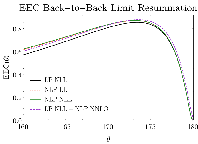
Figure 2: EEC as a function of $\theta$ in the back-to-back limit. We use $g^{2}/(4\pi)=0.118$ to mimic the QCD strong coupling at Z pole. The dashed line refers to LP resummed to NLL, with the inclusion of NLP terms up to NNLO ($n\leq 3$).

V Discussions

Our results lead to several exciting research avenues. First of all, it is interesting to apply the results to EEC in QCD, where fixed-order data up to NLO has become available recently Dixon et al. (2018); Luo et al. (2019); Gao et al. (2021). The local correlator of four electromagnetic currents in QCD has also been computed at one loop Chicherin et al. (2021). Secondly, in QCD running coupling corrections will modify NLL series. It would be important to understand how to incorporate these effects while retaining the power of conformal symmetry. Thirdly, our results provide concrete data for quantitative comparison between additive and multiplicative scheme in resummation matching, see e.g. Bizoń et al. (2018). Fourthly, local correlators exhibit other interesting limits, such as the Regge limit Costa et al. (2012). It would be interesting to understand what constraints are imposed on EEC by such limits. Last but not least, it would be worthwhile to understand the relation between our approach and the conventional approach based on momentum space renormalization group, in particular the relation between crossing symmetry for local correlator and the consistency relations from infrared poles cancellations Moult et al. (2017a).

Supplemental material

Appendix A Scalar Local Correlator

To make precise the local correlator in (4), we consider the following operator made out of the six scalars $\phi^{I=1,\ldots,6}$ of $\mathcal{N}=4$ SYM

$$O^{IJ}=\mathrm{tr}\left(\phi^{I}\phi^{J}\right)-\frac{1}{6}\delta^{IJ}\mathrm{tr}\left(\phi^{K}\phi^{K}\right)\,,$$ (S.1)

The operator is the superprimary of the stress tensor multiplet and transforms in the symmetric traceless representation of the $SO(6)$ R-symmetry group. It is convenient to keep track of the R-symmetry information by contracting the indices with null polarization vectors $Y_{I}$ or with a traceless symmetric tensor $S_{IJ}$

$$O(x,Y)\equiv O^{IJ}(x)Y_{I}Y_{J}\,,\quad\text{or}\quad O(x,S)=O^{IJ}(x)S_{IJ}\,.$$ (S.2)

Due to superconformal symmetry, the four-point function has following “partially non-renormalized” form Eden et al. (2001)

$$\langle O(x_{1},Y_{1})O(x_{2},Y_{2})O(x_{3},Y_{3})O(x_{4},Y_{4})\rangle=G^{(0)}(1,2,3,4)+\frac{2(N_{c}^{2}-1)}{(4\pi^{2})^{4}}\frac{y_{12}^{4}y_{34}^{4}}{x_{12}^{2}x_{34}^{2}x_{14}^{2}x_{23}^{2}}R\;\Phi(u,v)$$ (S.3)

where $G^{(0)}(1,2,3,4)$ is the tree-level correlator

$$G^{(0)}(1,2,3,4)= \frac{(N_{c}^{2}-1)^{2}}{4(4\pi^{2})^{4}}\left(\left(\frac{y_{12}^{2}y_{34}^{2}}{x_{12}^{2}x_{34}^{2}}\right)^{2}+\left(\frac{y_{13}^{2}y_{24}^{2}}{x_{13}^{2}x_{24}^{2}}\right)^{2}+\left(\frac{y_{41}^{2}y_{23}^{2}}{x_{41}^{2}x_{23}^{2}}\right)^{2}\right)$$ (S.4)

$$+\frac{N_{c}^{2}-1}{(4\pi^{2})^{4}}\left(\frac{y_{12}^{2}y_{23}^{2}y_{34}^{2}y_{41}^{2}}{x_{12}^{2}x_{34}^{2}x_{23}^{2}x_{41}^{2}}+\frac{y_{12}^{2}y_{24}^{2}y_{34}^{2}y_{13}^{2}}{x_{12}^{2}x_{24}^{2}x_{34}^{2}x_{31}^{2}}+\frac{y_{13}^{2}y_{23}^{2}y_{24}^{2}y_{41}^{2}}{x_{13}^{2}x_{23}^{2}x_{24}^{2}x_{41}^{2}}\right)\,,$$

with $y_{ij}^{2}\equiv Y_{i}\cdot Y_{j}$ and the function $\Phi(u,v)$ encodes all the dynamical information. The factor $R$ is determined by superconformal symmetry

$$R=(1-z\alpha)(1-z\bar{\alpha})(1-\bar{z}\alpha)(1-\bar{z}\bar{\alpha})\;,$$ (S.5)

where the conformal cross ratios $z$, $\bar{z}$ have already been introduced in the main text and $\alpha$, $\bar{\alpha}$ are similarly the R-symmetry cross ratios defined by

$$\frac{y_{13}^{2}y_{24}^{2}}{y_{12}^{2}y_{34}^{2}}=\alpha\bar{\alpha}\;,\quad\frac{y_{14}^{2}y_{23}^{2}}{y_{12}^{2}y_{34}^{2}}=(1-\alpha)(1-\bar{\alpha})\;.$$ (S.6)

The weak coupling $g\ll 1$ expansion of $\Phi(u,v)$ reads

$$\Phi(u,v)=\sum_{n=1}^{\infty}a^{n}\Phi^{(n)}(u,v)\,,\quad\quad a=\frac{g^{2}N_{c}}{4\pi^{2}}\;,$$ (S.7)

and is known up to three loops Drummond et al. (2013). Since the dynamic function $\Phi(u,v)$ is R-symmetry independent, we can choose special polarizations to simplify the correlator (S.3). Following Belitsky et al. (2014a), let us take

$$Y_{I}=(1,0,1,0,i,i)\,,\quad S_{IJ}=\mathrm{diag}(1,-1,0,0,0,0)\,,\quad S^{\prime}_{IJ}=\mathrm{diag}(0,0,1,-1,0,0)\,,$$ (S.8)

and define

$$\begin{split}&\widetilde{\mathcal{O}}(x_{2})=2O(x_{2},S)\,,\quad\widetilde{\mathcal{O}}^{\prime}(x_{4})=2O(x_{4},S^{\prime})\,,\\ &\mathcal{O}(x_{3})=\left(\frac{N_{c}^{2}-1}{2\pi^{4}}\right)^{-\frac{1}{2}}O(x_{3},Y)\,,\quad\mathcal{O}^{\dagger}(x_{1})=\left(\frac{N_{c}^{2}-1}{2\pi^{4}}\right)^{-\frac{1}{2}}O(x_{1},Y^{*})\,.\end{split}$$ (S.9)

Then the four-point function becomes

$$\begin{split}\langle\mathcal{O}^{\dagger}(x_{1})\widetilde{\mathcal{O}}(x_{2})\widetilde{\mathcal{O}}^{\prime}(x_{4})\mathcal{O}(x_{3})\rangle={}&\frac{1}{(2\pi)^{4}}\frac{1}{(x_{12}^{2}x_{34}^{2})^{2}}\left[\frac{N_{c}^{2}-1}{8}\left(1+\frac{u^{2}}{v^{2}}\right)+\frac{u}{v}\left(\frac{1}{2}+\Phi(u,v)\right)\right]\\ ={}&\frac{1}{(2\pi)^{4}}\frac{1}{(x_{12}^{2}x_{34}^{2})^{2}}\left(\frac{N_{c}^{2}-1}{8}G^{\text{short}}(u,v)+\frac{1}{u^{2}}\mathcal{F}(u,v)\right)\;,\end{split}$$ (S.10)

where we have further split it into short multiplet contribution $G^{\text{short}}(u,v)$ and the long multiplet contribution $\mathcal{F}(u,v)$. The explicit form of $G^{\text{short}}(u,v)$ can be found in Beem et al. (2017) and is protected from perturbative corrections. As a result, $\Phi(u,v)$ is essentially the same as all the loop corrections ($n\geq 1$) of $\mathcal{F}(u,v)=\sum_{n\geq 0}a^{n}\mathcal{F}^{(n)}(u,v)$, i.e.,

$$\mathcal{F}(u,v)-\mathcal{F}^{(0)}(u,v)=\frac{u^{3}}{v}\Phi(u,v)\,.$$ (S.11)

Another reason for choosing the polarizations (S.8) is the relation to the scalar detectors

$$\mathcal{S}(n_{i})=\frac{1}{4}\int\displaylimits_{-\infty}^{\infty}dn_{i}\cdot x_{i}\lim_{\bar{n}_{i}\cdot x_{i}\to\infty}(\bar{n}_{i}\cdot x_{i})^{2}\mathcal{O}(x_{i})\,.$$ (S.12)

Thanks to superconformal symmetry, the spinning correlator $\langle JTTJ\rangle$ is related to the scalar correlator (S.3) by Ward identities. Moreover, the EEC and the scalar-scalar correlation (SSC) are also proportional Belitsky et al. (2014a)

$$\langle\mathcal{E}(n_{2})\mathcal{E}(n_{4})\rangle=\frac{4(q^{2})^{2}}{(n_{2}\cdot n_{4})^{2}}\langle\mathcal{S}(n_{2})\mathcal{S}(n_{4})\rangle\,.$$ (S.13)

Appendix B Twist Conformal Blocks

The TCBs with logarithms can be computed using the method of Henriksson and Lukowski (2018). The idea is to apply the recursion relations on $\bar{H}_{\tau_{0}}^{(0,0)}(\bar{z})$, which is determined by the tree-level correlator, and compute $\bar{H}_{\tau_{0}}^{(m,0)}(\bar{z})$ at negative integer $m$. We then analytic continue in $m$ and take derivatives to obtain the logarithms. For our case, $\tau_{0}=2$ and we have

$$\bar{H}_{2}^{(0,0)}(\bar{z})=\frac{\bar{z}^{2}(2-\bar{z})}{2(1-\bar{z})}+\bar{z}\log(1-\bar{z})=\frac{1}{2\epsilon}+\text{regular terms }\,.$$ (S.14)

Repeated $\bar{D}$ action gives $\bar{H}_{2}^{(m,0)}(\bar{z})$ and the first few terms in small $\epsilon$ for negative integer $m$ are given by (3.37) of  Henriksson and Lukowski (2018)

$$\begin{split}\bar{H}^{(m,0)}_{2}(\bar{z})=&\frac{1}{2}\epsilon^{m-1}\Gamma(1-m)^{2}+\frac{1}{6}m\left(2m^{2}-6m+1\right)\epsilon^{m}\Gamma(-m)^{2}\\ &+\frac{1}{180}(m-1)m(m+1)\left(20m^{3}-54m^{2}-35m+36\right)\epsilon^{m+1}\Gamma(-m-1)^{2}+\cdots\,.\end{split}$$ (S.15)

Obtaining the full analytic expression for $\bar{H}^{(m,i)}_{2}(\epsilon)$ is difficult. But life is much easier if we content ourselves with getting first few orders in $\epsilon$ and logarithms. Truncated to order $\epsilon^{0}$, only $\bar{H}^{(0,i)}_{2}(\epsilon)$ and $\bar{H}^{(1,i)}_{2}(\epsilon)$ are relevant and we find

$$\bar{H}^{(0,i)}_{2}(\bar{z}) = \frac{(-1)^{i}}{\epsilon}\left[\frac{1}{2}\log^{i}\epsilon+i\gamma_{E}L^{i-1}_{\epsilon}+\frac{i(i-1)}{12}(12\gamma_{E}^{2}+\pi^{2})L^{i-2}_{\epsilon}+\cdots\right]$$

$$+ (-1)^{i}\left[\frac{1}{6(i+1)}L^{i+1}_{\epsilon}+\frac{\gamma_{E}-3}{3}L^{i}_{\epsilon}+\frac{\pi^{2}+12\gamma_{E}^{2}-72\gamma_{E}+12}{36}iL^{i-1}_{\epsilon}+\dots\right]+\cdots\,,$$

$$\bar{H}^{(1,i)}_{2}(\bar{z}) = (-1)^{i}\left[\frac{1}{2(i+1)(i+2)}L^{i+2}_{\epsilon}+\frac{\gamma_{E}}{i+1}L^{i+1}_{\epsilon}+\frac{12\gamma_{E}^{2}+\pi^{2}}{12}L^{i}_{\epsilon}+\cdots\right]+\cdots\,.$$ (S.17)

Appendix C More Details of (26) and (27)

In this section, we present the details of the large spin perturbation calculation needed for obtaining EEC in the back-to-back limit to the NLL and NLP order. As we explained in the main text, only twist-2 contributions are needed. The expansion of the twist-2 conformal block $\mathbf{G}_{2+\gamma_{2,\ell},\ell}(z,\bar{z})$ in the $z\to 0$ limit is

$$\begin{split}\mathbf{G}_{2+\gamma_{2,\ell},\ell}(z,\bar{z})&=z^{3+\gamma_{2,\ell}/2}k_{6+2\ell+\gamma_{2,\ell}}(\bar{z})+\mathcal{O}(z^{4})\\ &=z^{3}\sum_{n=0}^{\infty}a^{n}\Bigg{\{}\left[\frac{1}{2^{n}n!}\left(\gamma^{(1)}_{2,\ell}\right)^{n}\log^{n}z+\frac{1}{2^{n-1}(n-2)!}\gamma^{(2)}_{2,\ell}\left(\gamma^{(1)}_{2,\ell}\right)^{n-2}\log^{n-1}z+\cdots\right]k_{6+2\ell}(\bar{z})\\ &\qquad\qquad\qquad+\frac{1}{2^{n}(n-1)!}\left(\gamma^{(1)}_{2,\ell}\right)^{n}\log^{n-1}z\;\partial_{\ell}k_{6+2\ell}(\bar{z})+\cdots\Bigg{\}}+\mathcal{O}(z^{4})\,.\end{split}$$ (S.18)

Combined with the expansion of the OPE coefficient $a_{2,\ell}$, we obtain the leading twist contribution to $\mathcal{F}(z,\bar{z})$

$$\begin{split}\mathcal{F}^{(n)}(z,\bar{z})&=z^{3}\sum_{\text{even }\ell}\Bigg{\{}\log^{n}z\frac{1}{2^{n}n!}a^{(0)}_{2,\ell}\left(\gamma^{(1)}_{2,\ell}\right)^{n}k_{6+2\ell}(\bar{z})+\log^{n-1}z\Bigg{[}a^{(1)}_{2,\ell}\frac{\left(\gamma^{(1)}_{2,\ell}\right)^{n-1}}{2^{n-1}(n-1)!}+a^{(0)}_{2,\ell}\frac{\gamma^{(2)}_{2,\ell}\left(\gamma^{(1)}_{2,\ell}\right)^{n-2}}{2^{n-1}(n-2)!}\Bigg{]}k_{6+2\ell}(\bar{z})\\ &\qquad+\log^{n-1}z\;a^{(0)}_{2,\ell}\frac{1}{2^{n}(n-1)!}\left(\gamma^{(1)}_{2,\ell}\right)^{n}\partial_{\ell}k_{6+2\ell}(\bar{z})+\cdots\Bigg{\}}+\mathcal{O}(z^{4})\,,\end{split}$$ (S.19)

which is NLL in $\log z$. Then using the IBP identity

$$a^{(0)}_{2,\ell}\partial_{\ell}k_{6+2\ell}(\bar{z})=\partial_{\ell}[a^{(0)}_{2,\ell}k_{6+2\ell}(\bar{z})]-k_{6+2\ell}(\bar{z})\partial_{\ell}a^{(0)}_{2,\ell}\,,$$ (S.20)

and $a^{(1)}_{2,\ell}=-\zeta_{2}a^{(0)}_{2,\ell}+\frac{1}{2}\partial_{\ell}\left(a^{(0)}_{2,\ell}\gamma^{(1)}_{2,\ell}\right)$, we rewrite (S.19) as

$$\begin{split}\mathcal{F}^{(n)}(z,\bar{z})=&z^{3}\sum_{\text{even }\ell}\left\{\frac{1}{2^{n}n!}\log^{n}z\;a^{(0)}_{2,\ell}\left(\gamma^{(1)}_{2,\ell}\right)^{n}k_{6+2\ell}(\bar{z})\right.+\frac{1}{2^{n}(n-1)!}\log^{n-1}z\,\bigg{[}\left(\gamma^{(1)}_{2,\ell}\right)^{n}\partial_{\ell}\left(a^{(0)}_{2,\ell}k_{6+2\ell}(\bar{z})\right)\\ &\qquad\qquad\left.+a^{(0)}_{2,\ell}k_{6+2\ell}(\bar{z})\left(\gamma^{(1)}_{2,\ell}\right)^{n-2}\left[\left(-2\zeta_{2}+\partial_{\ell}\gamma^{(1)}_{2,\ell}\right)\gamma^{(1)}_{2,\ell}+2(n-1)\gamma^{(2)}_{2,\ell}\right]\bigg{]}+\cdots\right\}+\mathcal{O}(z^{4})\,.\end{split}$$ (S.21)

The use of (S.20) becomes clear when we use the integer-step finite difference to approximate $\partial_{\ell}\left(a^{(0)}_{2,\ell}k_{6+2\ell}(\bar{z})\right)$ at large spin $\ell$. On a general function $f(\ell)$, we approximate $f^{\prime}(\ell)\approx\frac{f(\ell+2)-f(\ell-2)}{4}$, which is accurate up to $\mathcal{O}(\ell^{-2})$. Neglecting boundary terms which vanish at large spins, we can write

$$\sum_{\text{even }\ell}\left(\gamma^{(1)}_{2,\ell}\right)^{n}\partial_{\ell}\left(a^{(0)}_{2,\ell}k_{6+2\ell}(\bar{z})\right)\approx\frac{1}{4}\sum_{\text{even }\ell}a^{(0)}_{2,\ell}k_{6+2\ell}(\bar{z})\left[\left(\gamma^{(1)}_{2,\ell-2}\right)^{n}-\left(\gamma^{(1)}_{2,\ell+2}\right)^{n}\right]\,,$$ (S.22)

Expanding everything other than $a_{2,\ell}^{(0)}$ with respect to the large conformal spin $J_{6,\ell}^{2}$, we get

$$\begin{split}\mathcal{F}^{(n)}(z,\bar{z})=z^{3}\sum_{\text{even }\ell}&\left\{\frac{1}{2^{n}n!}\log^{n}z\;a^{(0)}_{2,\ell}k_{6+2\ell}(\bar{z})\left[\left(\log(J_{6,\ell}^{2})+2\gamma_{E}\right)^{n}+\frac{n}{3}\left(\log(J_{6,\ell}^{2})+2\gamma_{E}\right)^{n-1}\frac{1}{J_{6,\ell}^{2}}+\cdots\right]\right.\\ &+\frac{1}{2^{n}(n-1)!}\log^{n-1}z\;a^{(0)}_{2,\ell}k_{6+2\ell}(\bar{z})\bigg{[}-(n+1)\zeta_{2}\left(\log(J_{6,\ell}^{2})+2\gamma_{E}\right)^{n-1}\\ &-3(n-1)\zeta_{3}\left(\log(J_{6,\ell}^{2})+2\gamma_{E}\right)^{n-2}+\frac{1}{J^{2}_{6,\ell}}\bigg{(}(n-1)\left(1-\frac{\zeta_{2}}{3}(n+1)\right)\left(\log(J_{6,\ell}^{2})+2\gamma_{E}\right)^{n-2}\\ &\left.\hskip 113.81102pt-(n-1)(n-2)\zeta_{3}\left(\log(J_{6,\ell}^{2})+2\gamma_{E}\right)^{n-3}\bigg{)}\bigg{]}+\cdots\right\}+\mathcal{O}(z^{4})\,,\end{split}$$ (S.23)

which can be organized into TCBs as

$$\begin{split}\mathcal{F}^{(n)}(z,\bar{z})=&\frac{\log^{n}z}{2^{n}n!}\left(\sum_{i=0}^{n}\frac{n!}{i!(n-i)!}(2\gamma_{E})^{i}H_{2}^{(0,n-i)}+\frac{n}{3}\sum_{i=0}^{n-1-i}\frac{(n-1)!}{i!(n-1-i)!}(2\gamma_{E})^{i}H_{2}^{(1,n-1-i)}+\cdots\right)\\ &+\frac{\log^{n-1}z}{2^{n}(n-1)!}\bigg{\{}-(n+1)\zeta_{2}\sum_{i=0}^{n-1}\frac{(n-1)!}{i!(n-1-i)!}(2\gamma_{E})^{i}H_{2}^{(0,n-1-i)}\\ &\qquad\qquad-3(n-1)\zeta_{3}\sum_{i=0}^{n-2}\frac{(n-2)!}{i!(n-2-i)!}(2\gamma_{E})^{i}H_{2}^{(0,n-2-i)}\\ &\qquad\qquad+(n-1)\left(1-\frac{\zeta_{2}}{3}(n+1)\right)\sum_{i=0}^{n-2}\frac{(n-2)!}{i!(n-2-i)!}(2\gamma_{E})^{i}H_{2}^{(1,n-2-i)}\\ &\qquad\qquad-(n-1)(n-2)\zeta_{3}\sum_{i=0}^{n-3}\frac{(n-3)!}{i!(n-3-i)!}(2\gamma_{E})^{i}H_{2}^{(1,n-3-i)}+\cdots\bigg{\}}+\cdots\,.\end{split}$$ (S.24)

Substituting the explicit TCBs (B, S.17), we get

$$\mathcal{F}^{(n)}(z,\bar{z}) =z^{3}\left\{\frac{1}{n!}\log^{n}z\left[\frac{1}{\epsilon}\left(\frac{(-1)^{n}}{2^{n+1}}\log^{n}\epsilon+\cdots\right)+\left(\frac{(-1)^{n+1}}{2^{n+1}}\log^{n}\epsilon+\frac{(-1)^{n}n}{3\times 2^{n}}\log^{n-1}\epsilon+\cdots\right)+\cdots\right]\right.$$ (S.25)

$$\qquad\quad+\frac{\log^{n-1}z}{(n-1)!}\bigg{[}\frac{1}{\epsilon}\left(\frac{(-1)^{n}}{2^{n+1}}(n+1)\zeta_{2}\log^{n-1}\epsilon-\frac{(-1)^{n}}{2^{n+1}}3(n-1)\zeta_{3}\log^{n-2}\epsilon+\cdots\right)$$

$$\left.\hskip 99.58464pt+\left(\frac{(-1)^{n}}{2^{n+1}n}\log^{n}\epsilon+\frac{(-1)^{n+1}}{2^{n+1}}(n+1)\zeta_{2}\log^{n-1}\epsilon+\cdots\right)\bigg{]}+\cdots\right\}+\mathcal{O}(z^{4})\,.$$

Via $\mathcal{F}^{(n)}(z,\bar{z})=\frac{v}{u^{3}}\Phi^{(n)}(z,\bar{z})$, this gives the expansion of $\Phi^{(n)}(z,\bar{z})$. Crossing symmetry allows us to further reconstruct the $\mathcal{O}(u^{1}v^{0})$ contributions, which gives the results in (29).

Appendix D Details of the Map from $u^{j_{1}}v^{j_{2}}L_{u}^{m}L_{v}^{n}$ to $y^{j}L_{y}^{k}$

In this section, we provide more details for establishing the map from the small $u,v$ expansion of $\Phi(u,v)$ to the small $y$ expansion of $\mathrm{EEC}(y)$. Instead of electromagnetic current sources $J_{\mu}$, we consider two scalar operator sources, belonging to the stress tensor multiplet, in the center of mass frame $q^{\mu}=(Q,0,0,0)$. $\mathrm{EEC}(y)$ relates to $\langle\mathcal{E}(n_{2})\mathcal{E}(n_{4})\rangle$ by an overall factor:

$$\mathrm{EEC}(y)=\int d\Omega_{2}d\Omega_{4}\delta(\vec{n}_{2}\cdot\vec{n}_{4}-\cos\theta)\frac{\langle\mathcal{E}(n_{2})\mathcal{E}(n_{4})\rangle}{Q^{2}}=\frac{8\pi^{2}}{Q^{2}}\langle\mathcal{E}(n_{2})\mathcal{E}(n_{4})\rangle\,,$$ (S.26)

where $\theta$ is the angle between $\vec{n}_{2}$ and $\vec{n}_{4}$ and we assume the convention that $\langle\mathcal{E}(n_{2})\mathcal{E}(n_{4})\rangle$ has already been normalized to the cross section. The superconformal Ward identities further reduce the EEC $\langle\mathcal{E}(n_{2})\mathcal{E}(n_{4})\rangle$ to scalar-scalar correlation (SSC) $\langle\mathcal{S}(n_{2})\mathcal{S}(n_{4})\rangle$  Belitsky et al. (2014a, c)

$$\langle\mathcal{E}(n_{2})\mathcal{E}(n_{4})\rangle=\frac{4(q^{2})^{2}}{(n_{2}\cdot n_{4})^{2}}\langle\mathcal{S}(n_{2})\mathcal{S}(n_{4})\rangle\,.$$ (S.27)

The SSC is related to the local correlator in a simple way in Mellin space Belitsky et al. (2014a)

$$\Phi(u,v)=\int\frac{dj_{1}dj_{2}}{(2\pi i)^{2}}M(j_{1},j_{2})u^{j_{1}}v^{j_{2}}\;.$$ (S.28)

Here $M(j_{1},j_{2})$ is the Mellin amplitude and encodes all the dynamical information. To compute the SSC, the first step is to obtain the Lorentzian correlator. This is achieved by using the Wightman prescription $x_{ij}^{2}\to-x_{ij}^{2}+i\epsilon t_{ij}$, if operator $i$ sits before $j$. In our case, the operator ordering is $1<2<4<3$. The second step is to perform the light transform on the Lorentzian correlator

$$\prod_{i=2,4}\int_{-\infty}^{\infty}d(n_{i}\cdot x_{i})\lim_{\bar{n}_{i}\cdot x_{i}\to\infty}\left(\frac{\bar{n}_{i}\cdot x_{i}}{2}\right)^{2}\,,$$ (S.29)

which turns local operators into detectors. To obtain SSC in the momentum space, the last step is the Fourier transformation $\int d^{4}x_{13}\exp(iq\cdot x_{13})$. After normalized to the total cross section, the Mellin representation for SSC is

$$\langle\mathcal{S}(n_{2})\mathcal{S}(n_{4})\rangle=\frac{1}{(2\pi)^{4}}\frac{\pi^{2}}{(n_{2}\cdot n_{4})q^{2}}\frac{1-y}{y}\int\frac{dj_{1}dj_{2}}{(2\pi i)^{2}}M(j_{1},j_{2})K(j_{1},j_{2};y)\,,$$ (S.30)

with

$$K(j_{1},j_{2};y)=\frac{2\Gamma(1-j_{1}-j_{2})}{\Gamma(j_{1}+j_{2})\left[\Gamma(1-j_{1})\Gamma(1-j_{2})\right]^{2}}\left(\frac{y}{1-y}\right)^{j_{1}+j_{2}}\,.$$ (S.31)

Then using $n_{2}\cdot n_{4}=2(1-y)$ in the center of mass frame, we obtain the Mellin representation for $\mathrm{EEC}(y)$

$$\mathrm{EEC}(y)=\frac{8\pi^{2}Q^{2}}{(1-y)^{2}}\langle\mathcal{S}(n_{2})\mathcal{S}(n_{4})\rangle=\frac{1}{4y(1-y)^{2}}\int\frac{dj_{1}dj_{2}}{(2\pi i)^{2}}M(j_{1},j_{2})K(j_{1},j_{2};y)\,.$$ (S.32)

Therefore, we expect the following mapping from the double lightcone limit to back-to-back limit

$$u^{j_{1}}v^{j_{2}}\to\frac{K(j_{1},j_{2};y)}{4y(1-y)^{2}}\,.$$ (S.33)

At LP and NLP, we need the following rules containing logarithms in $u,v$

$$\log^{m}u\log^{n}v \;\to\; m!\,n!\oint_{|j_{1}|=\epsilon}\frac{dj_{1}}{2\pi i}\frac{1}{j_{1}^{m+1}}\oint_{|j_{2}|=\epsilon}\frac{dj_{2}}{2\pi i}\frac{1}{j_{2}^{n+1}}\frac{K(j_{1},j_{2};y)}{4y(1-y)^{2}}\,,$$ (S.34)

$$u\log^{m}u\log^{n}v \;\to\; {m!\,n!}\oint_{|j_{1}-1|=\epsilon}\frac{dj_{1}}{2\pi i}\frac{1}{(j_{1}-1)^{m+1}}\oint_{|j_{2}|=\epsilon}\frac{dj_{2}}{2\pi i}\frac{1}{j_{2}^{n+1}}\frac{K(j_{1},j_{2};y)}{4y(1-y)^{2}}\,,$$ (S.35)

$$v\log^{m}u\log^{n}v \;\to\; {m!\,n!}\oint_{|j_{1}|=\epsilon}\frac{dj_{1}}{2\pi i}\frac{1}{j_{1}^{m+1}}\oint_{|j_{2}-1|=\epsilon}\frac{dj_{2}}{2\pi i}\frac{1}{(j_{2}-1)^{n+1}}\frac{K(j_{1},j_{2};y)}{4y(1-y)^{2}}\,.$$ (S.36)

For the cases we will inspect, the only exception is the constant term at NLP which is caused by the $j_{1}+j_{2}=1$ pole in $K(j_{1},j_{2};y)$. To see this, we consider the first derivative of $\frac{1-y}{y}K(j_{1},j_{2};y)$ w.r.t. $\frac{y}{1-y}$. Such an action shifts $\Gamma(1-j_{1}-j_{2})$ to $\Gamma(2-j_{1}-j_{2})$, which is analytic at $j_{1}+j_{2}=1$. The constant term is killed after taking the derivative, while the logarithmic information remains. The explicit expressions for general $m,n$ up to NLL accuracy are shown in Table 2.

Appendix E Comparison with Existing Results

In this section we provide a comparison of our predictions with the existing results in the literature. We begin with the local correlator in the double lightcone limit to NLL accuracy. The full three-loop correlator can be found in Drummond et al. (2013). Upon expanding their results in the double lightcone limit we find

$$\Phi^{(1)}(u,v) = \left[-\frac{1}{4}\log u\log v+0\cdot\log(uv)+\cdots\right]-{\color[rgb]{1,0,0}\left[\frac{1}{4}(u+v)\log u\log v+\frac{1}{2}(u\log u+v\log v)+\cdots\right]}+\cdots\,,$$

$$\Phi^{(2)}(u,v) = \left[\frac{1}{16}\log^{2}u\log^{2}v+0\cdot\log u\log v\log(uv)+\cdots\right]+\left[\frac{1}{8}(u+v)\log^{2}u\log^{2}v\right.$$

$$\qquad\left.+\frac{3}{16}\log u\log v(u\log u+v\log v)+{\color[rgb]{1,0,0}\frac{1}{8}\log u\log v(v\log u+u\log v)}+\cdots\right]+\cdots\,,$$

$$\Phi^{(3)}(u,v) = \left[-\frac{1}{96}\log^{3}u\log^{3}v+0\cdot\log^{2}u\log^{2}v\log(uv)+\cdots\right]-\left[\frac{1}{48}(u+v)\log^{3}u\log^{3}v\right.$$ (S.37)

$$\left.\qquad+\frac{1}{24}\log^{2}u\log^{2}v(u\log u+v\log v)+\frac{1}{48}\log^{2}u\log^{2}v(v\log u+u\log v)+\cdots\right]+\cdots\,.$$

Compared with our NLL prediction (29), we find perfect agreement except for the NLP terms at one loop and a single NLL-NLP term at two loops (shown in red explicitly). Such terms do not correspond to enhanced divergence in $v$ and hence cannot be captured by the large spin analysis. Moreover, the two-loop NLL-NLP mismatched term ${\color[rgb]{1,0,0}\frac{1}{8}\log u\log v(v\log u+u\log v)}$ does not map to NLL-NLP term in EEC, as can be checked from Table 2.

For EEC in ${\cal N}=4$ SYM results up to three loops with full $y$ dependence have been computed in Henn et al. (2019), using the local correlator from Drummond et al. (2013) as input. The back-to-back expansion of Henn et al. (2019) up to NLL at NLP is

$$\mathrm{EEC}^{(1)} = -\frac{1}{4y}\log y{\color[rgb]{1,0,0}-\frac{1}{2}\log y}{\color[rgb]{1,0,0}+0\cdot y^{0}}+\mathcal{O}(y)\,,$$

$$\mathrm{EEC}^{(2)} = \frac{1}{y}\left(\frac{\log^{3}y}{8}+0\cdot\log^{2}y+\cdots\right)+\left(\frac{\log^{3}y}{6}+\frac{3}{16}\log^{2}y+\cdots\right)+\mathcal{O}(y)$$

$$\mathrm{EEC}^{(3)} = \frac{1}{y}\left(-\frac{\log^{5}y}{32}+0\cdot\log^{4}y+\cdots\right)+\left(-\frac{3\log^{5}y}{80}-\frac{\log^{4}y}{12}+\cdots\right)+\mathcal{O}(y)\,.$$ (S.38)

To obtain (S.38), it is necessary to expand the following integral to NLP,

$$\mathrm{E}=\int_{0}^{1}d\bar{z}\int_{0}^{\bar{z}}dt\frac{-1}{t(1-y-\bar{z})+y\bar{z}}\left[\frac{z\bar{z}}{1-z-\bar{z}}P_{1}+\frac{z^{2}\bar{z}}{(1-z)^{2}(1-z\bar{z})}P_{2}\right]\,,$$ (S.39)

where $z=(1-y)t(t-\bar{z})/(t(1-y-\bar{z})+y\bar{z})$ and $P_{1}$ and $P_{2}$ are lengthy combinations of weight-3 harmonic polylogarithms and can be found in Henn et al. (2019). The expansion of this integral begins from NLP and reads

$$\mathrm{E}=\frac{\log^{5}y}{60}+0\cdot\log^{4}y+\frac{1}{12}\zeta_{2}\log^{3}y+\cdots$$ (S.40)

where we have neglected terms of ${\cal O}(\log^{2}y)$ and beyond. The expansion of this integral was also performed in Moult et al. (2020b), but the result reported in Eq. (5.17) of Moult et al. (2020b) is larger than (S.40) by a factor of two. Using (S.40) and expanding the remaining results in Henn et al. (2019) with the package HPL, we obtain $\mathrm{EEC}^{(3)}$ presented in (S.38).

Our results in (32) for $n>1$ are in full agreement with $\mathrm{EEC}^{(2)}$ and $\mathrm{EEC}^{(3)}$ in (S.38). This provides a strong check for our results. Our large spin analysis does not expect to capture the NLP terms at one loop (shown in red in (S.38)), for the same reason as explained for local correlator.

We note that a LL study at NLP has also been performed in Moult et al. (2020b), where an RG equation at NLP has been derived. After changing to our normalization, their predicted LL coefficient at NLP and three loop, given in Eq. (5.21) of Moult et al. (2020b), is $-1/30\log^{5}y$, which disagrees with our results in (33), as well as with the full results from Henn et al. (2019).