Study of the de Almeida-Thouless (AT) line in the one-dimensional diluted power-law XY spin glass

Abstract

We study the AT line in the one-dimensional power-law diluted XY spin glass model, in which the probability that two spins separated by a distance $r$ interact with each other, decays as $1/r^{2\sigma}$. Tuning the exponent $\sigma$ is equivalent to changing the space dimension of a short-range model. We develop a heat bath algorithm to equilibrate XY spins; using this in conjunction with the standard parallel tempering and overrelaxation sweeps, we carry out large scale Monte Carlo simulations. For $\sigma=0.6$, which is in the mean-field regime above six dimensions – it is similar to being in 10 dimensions – we find clear evidence for an AT line. For $\sigma=0.75$ and $\sigma=0.85$, which are in the non-mean-field regime and similar to four and three dimensions respectively, our data is like that found in previous studies of the Ising and Heisenberg spin glasses when reducing the temperature at fixed field. For $\sigma=0.75$, there is evidence from finite size scaling studies for an AT transition but for $\sigma=0.85$, the evidence for a transition is non-existent. We have also studied these systems at fixed temperature varying the field and discovered that at both $\sigma=0.75$ and at $\sigma=0.85$ there is evidence of an AT transition! Confusingly, the correlation length and spin glass susceptibility as a function of the field are both entirely consistent with the predictions of the droplet picture and hence the non-existence of an AT line. In the usual finite size critical point scaling studies used to provide evidence for an AT transition, there is seemingly good evidence for an AT line at $\sigma=0.75$ for small values of the system size $N$, which is strengthening as $N$ is increased, but for $N>2048$ the trend changes and the evidence then weakens as $N$ is further increased. We have also studied with fewer bond realizations the system at $\sigma=0.70$, which is the analogue of a system with short-range interactions just below six dimensions, and found that it is similar in its behavior to the system at $\sigma=0.75$ but with larger finite size corrections. The evidence from our simulations points to the complete absence of the AT line in dimensions outside the mean-field region and to the correctness of the droplet picture. Previous simulations which suggested there was an AT line can be attributed to the consequences of studying systems which are just too small. The collapse of our data to the droplet scaling form is poor for $\sigma=0.75$ and to some extent also for $\sigma=0.85$, when the correlation length becomes of the order of the length of the system, due to the existence of excitations which only cost a free energy of $O(1)$, just as envisaged in the TNT picture of the ordered state of spin glasses. However, for the case of $\sigma=0.85$ we can provide evidence that for larger system sizes, droplet scaling will prevail even when the correlation length is comparable to the system size.

I Introduction

While the spin glass problem at mean-field level is now well-understood [1], questions remain as to the nature of the ordered state in three dimensional spin glasses. A key question is whether the ordered phase of real spin glasses has the broken replica symmetry features found in mean-field theory. This question is most easily answered by finding whether on application of a magnetic field $h_{r}$ there is a line, the so-called de Almeida Thouless (AT) line [2], below which in the $h_{r}-T$ plane there is replica symmetry breaking. This line exists at mean-field level (see Fig. 1) and its possible existence in three dimensions can be studied experimentally and with simulations. Simulational studies of the existence of replica symmetry breaking within the zero-field spin glass state itself are plagued by finite size effects: it is expected that the difference between the predictions of droplet scaling and those of replica symmetry breaking will only become visible for very large systems (for a review see [3]). A recent review of simulations, including studies of the existence of the AT line, can be found in Ref. [4].

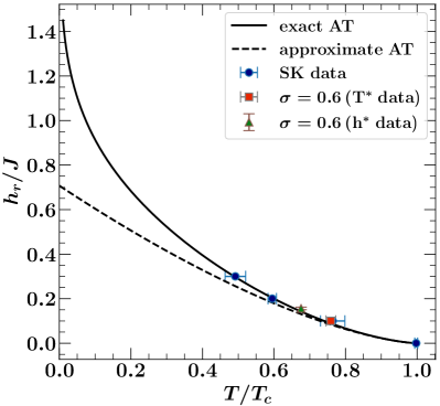
Figure 1: The AT line. The solid line is the exact AT line for the SK model, calculated as in Ref. [5]. The dashed line is the approximation to it of Eq. (8). We have marked on the diagram the results of our simulations on the SK model, which were done to check our Monte Carlo procedures. The points in red and green are the results of our simulations at $\sigma=0.6$, which lie in the mean-field region. The data on the horizontal axis for $\sigma=0.6$ are normalized to the transition temperature $T_{c}$ in zero field for that value of $\sigma$. For the XY SK model the AT line goes to infinity as $T\to 0$.

Right from the early days of spin glass studies there have been doubts raised as to whether the AT line existed below six dimensions. For example Bray and Roberts  [6] attempted to do an expansion in $6-\epsilon$ dimensions for the critical exponents at the AT line but failed to find a stable fixed point. They suggested that maybe that indicated that there might be no AT line below six dimensions. A renormalization group calculation also gave indications that the AT line was going away as $d\to 6$ from above  [7]. As it is difficult to do simulations in dimensions around $6$ to check these speculations, simulators have had to turn instead to one-dimensional models with long-range power-law interactions.

These models go back to Kotliar, Anderson and Stein [8], who in turn were inspired by the long-range ferromagnet that was studied by Dyson [9, 10]. The long-range power-law model has the advantage that by tuning the power-law exponent $\sigma$, one has access to both the mean-field and the regimes with non-mean-field critical behavior. However, the full power-law model is expensive for numerics. Fortunately a clever workaround was introduced by Leuzzi et al. [11] where instead of the interactions falling off as a power law, it is the probability of there being a bond between two spins that falls off as a power law. The fewer bonds in the model means that a significantly smaller computational cost is involved, thus allowing for the simulation of larger system sizes.

While the vast literature on spin glasses is mostly focussed on Ising spins [11, 12, 13, 14, 15, 16], there has been a revival of interest in classical $m$-component vector spin glass models [5, 17, 18, 19, 20, 21, 22, 23, 24, 25, 26] in the last decade or so. The XY model has $m=2$ and the Heisenberg model has $m=3$. One of the triggers for this revival has been the finding that the infinite-range vector spin glass exhibits an AT line provided a magnetic field that is random in all the component directions is applied [5]. Furthermore analytical studies of the AT transition in $m$-vector models shows that the field theory of these AT transitions is that of the Ising spin glass  [5]. Thus it has become possible to study the question of whether or not an Ising AT transition exists in various dimensions by studying one-dimensional vector spin glasses with long-range interactions  [18]!

In this paper, we study the one-dimensional diluted XY spin glass subjected to a random vector magnetic field, with the aid of large scale Monte Carlo simulations. While Monte Carlo simulations are a time-tested tool for the study of phase transitions in spin glasses, the exorbitant cost of equilibration makes them rather challenging in practice. It has been argued that vector spins tend to equilibrate faster compared to Ising spins [27], because of the soft nature of the spins involved, even though the presence of more components adds to the cost. The Heisenberg spin glass [19, 18, 17, 5, 27, 28, 29, 30, 31, 32] has been the popular vector spin to have been considered, because of the availability of the heatbath algorithm [28], which works very efficiently to equilibrate it. The XY spin glass is less effectively handled by the heatbath algorithm [33, 34] because of the technicalities involved in inverting a probability distribution for which a simple closed form expression is unavailable in the XY case. In this paper, we develop a method, which is outlined in Appendix A to perform this inversion numerically with the hope of benefiting from the vector nature of XY spins, while simultaneously reducing the components to as small a number as possible.

The improved algorithm yields mixed fruits. The gains from the reduced number of components seems to be largely counterbalanced by the additional resources consumed by the numerical inversion. However, with the aid of extensive computational power, we are able to access system sizes comparable to those in the corresponding study with Heisenberg spins. Our findings for the XY diluted spin glass closely mimic those obtained for the Heisenberg version of the same model [18, 17, 5] and the Ising spin glass in three dimensions [35] when we investigate crossing the possible AT line by varying $T$ at fixed values of $h_{r}$. In the mean-field regime, (we studied here the case of $\sigma=0.6$, which corresponds to $10$ dimensions, which is above the upper critical dimension of $6$), there is clear evidence of an Almeida-Thouless line (see Sec. V.1). There is rather weak evidence for an Almeida-Thouless line for $\sigma=0.85$ using the commonly employed finite size critical point scaling methods of analysis (see Sec. V.3). At this value of $\sigma$, our system should be similar to the Edwards-Anderson model in three dimensions with short-range interactions. For the in-between case at $\sigma=0.75$ which lies in the non-mean-field regime, but closer to the mean-field boundary at $\sigma=2/3$, our data do provide stronger evidence for a phase transition in the presence of small magnetic fields than at $\sigma=0.85$. However, by varying the magnetic field $h_{r}$ at fixed temperature $T$ we find in Sec. V that at both $\sigma=0.75$ and at $\sigma=0.85$ there is quite decent evidence for an AT line. Confusingly, the field dependence of the correlation length is very well-described by the Imry-Ma prediction of the droplet picture, which implies the complete absence of the AT transition! In the droplet picture the correlation length in a field remains finite and only diverges as $h_{r}\to 0$. However, when this correlation length becomes comparable to the system size $L$ the Imry-Ma formula needs to be modified and we give in Sec. VI a scaling form for this modification. It is based upon the usual finite size scaling approach used in studying critical phenomena, and just as for critical phenomena we find that there are finite size corrections to this scaling form. In addition to these scaling corrections there are corrections which arise when $\xi_{\text{SG}}\sim L<L^{*}$ which are of different origin and are connected to TNT effects [36, 37]. TNT effects arise from droplets whose linear dimension $L$ is of the order of the system size with free energy cost of $O(1)$ (rather than the $L^{\theta}$ of the droplet picture), and exist in systems whose sizes $L<L^{*}$ [3]. The length scale $L^{*}$ is always large and is expected to diverge as $d\to 6$ or as $\sigma\to 2/3$. It is only for the case of $\sigma=0.85$ that we can reach sizes where TNT effects seem to be getting small. These matters are discussed in Sec. VII.

Furthermore, we can use the droplet scaling picture to explain some of the features of the apparent AT transition which arise on performing the usual finite size critical scaling analyses, and show that these are the consequence of not studying large enough systems. Unfortunately these arguments will only become compelling for system sizes which we cannot reach. Our chief evidence for the droplet picture is its very successful prediction of the correlation length as a function of the field in the region when finite size and TNT effects are unimportant.

Our claim that the evidence favors the absence of the AT line for values of $\sigma$ outside the mean-field region is consistent with the attempt [21] to calculate the AT field at $T=0$ using an expansion in $1/m$. This indicated that as $d\to 6$ from above in the Edwards-Anderson model, the AT field would go to zero, implying the absence of the AT line below $6$ dimensions (which in the one-dimensional long-range model corresponds to $2/3<\sigma<1$). For $\sigma>1$ there is no finite temperature spin glass phase.

The plan of this paper is as follows. In Sec. II we describe the model in detail. In Sec. III we describe the quantities which were studied in our Monte Carlo simulations, the details of which are given in Appendix A. Our data is analysed in Sec. V on the assumption that there is an AT transition, while in Sec. VI the data is analysed according to droplet scaling assumptions. In Sec. VII we discuss the effect of TNT behavior on our results. Finally in Sec. VIII we summarize our conclusions.

II Model Hamiltonian

The general Hamiltonian for vector spin glasses is:

$$\mathcal{H}=-\sum\limits_{\langle i,j\rangle}J_{ij}\textbf{S}_{i}\cdot\textbf{S}_{j}-\sum\limits_{i}\textbf{h}_{i}\cdot\textbf{S}_{i}\,,$$ (1)

where $\textbf{S}_{i}$ is the spin on the $i^{\text{th}}$ lattice site ($i=1,2,\ldots,N$), which is chosen to be a unit vector. $m$ represents the number of components of the vector $\textbf{S}_{i}$. In this work we concentrate on XY spins, and set $m=2$. The Cartesian components $h_{i}^{\mu}$ ($\mu=1,2$) of the on-site external magnetic field are i.i.d random variables drawn from a Gaussian distribution of zero mean and variance $h_{r}^{2}$ and satisfy the relation:

$$\left[h_{i}^{\mu}h_{j}^{\nu}\right]_{\text{av}}=h_{r}^{2}\delta_{ij}\delta_{\mu\nu}.$$ (2)

We use the notation $\langle\cdots\rangle$ for thermal average and $[\cdots]_{\text{av}}$ for an average over quenched disorder throughout this paper.

The spins are arranged on a circle so the geometric distance between a pair of spins $(i,j)$ is given by [16]

$$r_{ij}=\frac{N}{\pi}\sin\left(\frac{\pi}{N}\left|i-j\right|\right),$$ (3)

which is the length of the chord connecting the $i^{\text{th}}$ and $j^{\text{th}}$ spins. The interactions $J_{ij}$ are independent random variables such that the probability of having a non-zero interaction between a pair of spins $(i,j)$ falls with the distance $r_{ij}$ between the spins as a power law:

$$P(J_{ij})\propto\frac{1}{r_{ij}^{2\sigma}}.$$ (4)

If the spins $i$ and $j$ are linked the magnitude of the interaction between them is drawn from a Gaussian distribution whose mean is zero and whose standard deviation is unity, i.e:

$$\left[J_{ij}\right]_{\text{av}}=0\qquad\text{and}\qquad\left[J_{ij}^{2}\right]_{\text{av}}=J^{2}=1.$$ (5)

The mean number of non-zero bonds from a site is fixed to be $\tilde{z}$ (co-ordination number). So, the total number of bonds among all the spins on the lattice is fixed to be $N_{b}=N\tilde{z}/2$. When $\tilde{z}=6$ this model mimics the 3D simple cubic lattice model and we use this value for $\tilde{z}$ for all the $\sigma$ values studied. (For $\sigma=0$ and $\tilde{z}=N-1$, the model becomes the infinite-range Sherrington-Kirkpatrick (SK) model [38]).

To generate the set of interaction pairs [11, 17] $(i,j)$ with the desired probability we pick a site $i$ randomly and uniformly and then choose a second site $j$ with probability given by:

$$p_{ij}=\frac{r_{ij}^{-2\sigma}}{\sum\limits_{j\neq i}r_{ij}^{-2\sigma}}.$$ (6)

If the spins at $i$ and $j$ are already connected we repeat this process until we find a pair of sites $(i,j)$ which have not been connected. Once we find such a pair of spins, we connect them with a bond whose strength $J_{ij}$ is a Gaussian random variable with attributes given by Eq. (5). We repeat this process exactly $N_{b}$ times to generate $N_{b}$ pairs of interacting spins.

The advantage of the diluted model over the fully connected model is that, in a fully connected model, there are $N(N-1)/2$ interactions. The ratio of the number of interactions of the diluted model to the fully connected model is $\tilde{z}/N$ which is a very small value as $N$ becomes large. Hence it is possible to go to much larger system sizes with a diluted model as compared to a fully connected model.

Figure 2: Finite size scaling analyses of data for $\sigma=0.60$ obtained by fixing the field and varying the temperature. The zero-field data are presented in the first row and the data with $h_{r}=0.1$ are shown in the second row. Figures (a) and (d) show the plots of $\chi_{\text{SG}}/N^{1/3}$ as a function of the temperature $T$ for different system sizes, with $h_{r}=0$ and $h_{r}=0.1$ respectively. The corresponding data for $\xi_{\text{SG}}/N^{d_{\text{eff}}/6}$ are shown in figures (b) and (e), with $d_{\text{eff}}=2/(2\sigma-1)$ in the mean-field regime (Eq. (9)). The exponents of $N$ are chosen according to Eqs. (14b) and (19b). Both the sets of plots show that the curves for different system sizes intersect. The data for the intersection temperatures $T^{*}(N,2N)$ between pairs of adjacent system sizes for $\chi_{\text{SG}}/N^{1/3}$ and $\xi_{\text{SG}}/N^{d_{\text{eff}}/6}$ are plotted as a function of $N^{-\lambda}$ in figures (c) and (f), for $h_{r}=0$ and $h_{r}=0.1$ respectively. The value of the exponent $\lambda$ is fixed to be $0.467$ which is known exactly in the mean-field regime [17, 39]. For $h_{r}=0$, the fits give $T_{c}=0.8873\pm 0.0017$ from $\chi_{\text{SG}}$ and $T_{c}=0.8893\pm 0.0046$ from $\xi_{\text{SG}}$. For $h_{r}=0.1$, both the datasets are consistent with a spin glass transition temperature of $T_{\text{AT}}(h_{r}=0.1)=0.67$.

At zero-field, the mean-field spin glass transition temperature for the $m$-component vector spin glass is given by [40, 17, 18]

$$T_{c}^{\text{MF}}=\frac{1}{m}\left(\sum_{j}\left[J_{ij}^{2}\right]_{\text{av}}\right)^{1/2}=\frac{\sqrt{\tilde{z}}}{m}J.$$ (7)

The approximate location of the AT line for an $m$-component infinite-range spin glass near the zero-field transition temperature $T_{c}$ is [5]

$$\left(\frac{h_{r}}{J}\right)^{2}=\frac{4}{m(m+2)}\left(1-\frac{T}{T_{c}}\right)^{3}.$$ (8)

The accuracy of this approximation for the SK model can be judged from Fig. 1.

A one-dimensional chain with power law diluted interactions for a particular value of $\sigma$ is equivalent to a short-range model [15, 39] of effective dimension $d_{\text{eff}}$, where

$$d_{\text{eff}}=\frac{2}{2\sigma-1},$$ (9)

i.e., there is a one-to-one mapping between a long-range diluted network with exponent $\sigma$ and a short-range model with space dimension $d_{\text{eff}}$, at least when $1/2<\sigma<2/3$. Thus when $\sigma=0.60$, $d_{\text{eff}}=10$. For the interval $2/3<\sigma<1$ other relations are required  [15, 41]. For example, for Ising spin glasses, it was suggested in Ref.  [41] that $d=4$ corresponded to $\sigma\approx 0.790$, while $d=3$ corresponded to $\sigma\approx 0.896$. Unfortunately, the mapping for the XY model has been less studied.

Figure 3: Finite size scaling analyses of $\chi_{\text{SG}}$ data (figure (a)), and $\xi_{\text{SG}}$ data (figure (b)), for $\sigma=0.60$ obtained by fixing the temperature to $T=0.6$ $(=0.67\,T_{c})$ and varying the field. Both the plots show that the curves for different system sizes intersect. Figure (c) shows the data for the intersection fields $h^{*}(N,2N)$ between pairs of adjacent system sizes, plotted as a function of $N^{-\lambda}$. Both the datasets are consistent with a spin glass transition at $h_{\text{AT}}(T=0.6)\approx 0.16$.

III Correlation lengths and susceptibilities

In this section we discuss the quantities which were obtained from our Monte Carlo simulations and used to extract a correlation length $\xi_{\text{SG}}$ and the spin glass susceptibility $\chi_{\text{SG}}$. The simulations themselves are described in detail in Appendix A.

The thermal average of a quantity is calculated using multiple replicas in the following standard way:

$$\langle A\rangle\langle B\rangle\langle C\rangle\langle D\rangle=\langle A^{(1)}B^{(2)}C^{(3)}D^{(4)}\rangle$$ (10)

where (1),(2),(3), and (4) are four copies of the system at the same temperature, and $A$,$B$,$C$, and $D$ are the quantities over which we would like to perform thermal averaging. The wave-vector-dependent spin glass susceptibility is given by [5]

$$\chi_{\text{SG}}(k)=\frac{1}{N}\sum\limits_{i,j}\frac{1}{m}\sum\limits_{\mu,\nu}\left[\left(\chi_{ij}^{\mu\nu}\right)^{2}\right]_{\text{av}}e^{ik(i-j)},$$ (11)

where

$$\chi_{ij}^{\mu\nu}=\left\langle S_{i}^{\mu}S_{j}^{\nu}\right\rangle-\left\langle S_{i}^{\mu}\right\rangle\left\langle S_{j}^{\nu}\right\rangle.$$ (12)

The spin glass correlation length is then determined from

$$\xi_{\text{SG}}=\frac{1}{2\sin(k_{\text{min}}/2)}\left(\frac{\chi_{\text{SG}}(0)}{\chi_{\text{SG}}\left(k_{\text{min}}\right)}-1\right)^{1/(2\sigma-1)}$$ (13)

where $k_{\text{min}}=(2\pi/N)$.

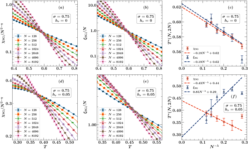
Figure 4: Finite size scaling analyses of data for $\sigma=0.75$ obtained by varying the temperature at fixed field. Figures in first row show the data generated at zero-field, where as the figures in second row show the data obtained by turning on a magnetic field of $h_{r}=0.05$. Figures (a) and (d) show data for $\chi_{\text{SG}}/N^{2-\eta}$ (with $2-\eta=2\sigma-1$) for different system sizes. Figures (b) and (e) show the corresponding data for $\xi_{\text{SG}}/N$. According to Eqs. (14a) and (19a) the data should intersect at $T_{\text{AT}}(h_{r})$, which is shown in figures (c) and (f) for $h_{r}=0$ and $h_{r}=0.05$ respectively. The $T^{*}(N,2N)$ data shown in these figures did not fit well with Eq. (17). So we used the value of the scaling exponent $\lambda=0.26$ obtained from the $h^{*}(N,2N)$ data (see Table 1), and fitted the $T^{*}(N,2N)$ data against $N^{-\lambda}$ using a straight line. The resulting values for the zero-field transition temperature are $T_{c}=0.6200\pm 0.0031$ from $\chi_{\text{SG}}$ and $T_{c}=0.6244\pm 0.0098$ from $\xi_{\text{SG}}$. For $h_{r}=0.05$ the linear fitting gives $T_{\text{AT}}(h_{r}=0.05)=0.4395\pm 0.0241$ from $\chi_{\text{SG}}$ and $T_{\text{AT}}(h_{r}=0.05)=0.2893\pm 0.0252$ from $\xi_{\text{SG}}$, and the values do not agree with each other.

IV Finite-size analyses assuming a transition exists

In this section we detail the method of finite-size analysis when a transition is assumed to exist. When studying the AT line, which is a line of phase transitions in the $h_{r}-T$ plane, it can be crossed on an infinite number of trajectories. The most commonly used trajectory is the one where $h_{r}$ is kept constant and the temperature $T$ is varied. In this work we also consider the trajectory in which $T$ is kept constant and $h_{r}$ is varied. We refer to the zero-field transition temperature as $T_{c}$ while we denote a generic transition temperature on the AT line by $T_{\text{AT}}(h_{r})$. Similarly we denote the field on the AT line by $h_{\text{AT}}(T)$.

The spin glass susceptibility $\chi_{\text{SG}}\equiv\chi_{\text{SG}}(0)$ of a finite system of $N$ spins has the finite size scaling form (near the transition temperature $T_{\text{AT}}(h_{r})$) [5]:

$$\frac{\chi_{\text{SG}}}{N^{2-\eta}} =\mathcal{C}\left[N^{1/\nu}\left(T-T_{\text{AT}}(h_{r})\right)\right],\quad(2/3\leq\sigma<1),$$ (14a)

$$\frac{\chi_{\text{SG}}}{N^{1/3}} =\mathcal{C}\left[N^{1/3}\left(T-T_{\text{AT}}(h_{r})\right)\right],\quad(1/2<\sigma\leq 2/3),$$ (14b)

where $\eta$ is given by $2-\eta=2\sigma-1$. These forms are examples of finite size scaling expressions which would be expected to hold in the critical region when $N\to\infty$, $(T-T_{\text{AT}}(h_{r}))\to 0$, with (say) $N^{1/\nu}(T-T_{\text{AT}}(h_{r}))$ finite. The scaling function $\mathcal{C}$ will depend on the value of $\sigma$. There are always finite size corrections to these forms. For example, the corrections to Eq. (14b) will be of the form

$$\frac{\chi_{\text{SG}}}{N^{1/3}} = \mathcal{C}\left[N^{1/3}\left(T-T_{\text{AT}}(h_{r})\right)\right]$$ (15)

$$+ N^{-\omega}\mathcal{G}\left[N^{1/3}(T-T_{\text{AT}}(h_{r}))\right].$$

It has been suggested [17, 39] that the correction to scaling exponent is given at least in the mean-field region by

$$\omega=1/3-(2\sigma-1).$$ (16)

Curves of $\chi_{\text{SG}}/N^{2-\eta}$ ($\chi_{\text{SG}}/N^{1/3}$ in the mean-field regime) plotted for different system sizes should intersect at the transition temperature $T_{\text{AT}}(h_{r})$. In reality, finite-size corrections to Eq. (14) are always present and cause the intersection point between the curves for size $N$ and $2N$ to depend on $N$. The intersection temperatures vary as [39, 42, 43, 44]

$$T^{*}(N,2N)=T_{\text{AT}}(h_{r})+\frac{A}{N^{\lambda}},$$ (17)

where $A$ is the amplitude of the leading correction, and the exponent $\lambda$ is

$$\lambda =1/3+\omega,\quad(1/2<\sigma\leq 2/3),$$ (18a)

$$\lambda =1/\nu+\omega,\quad(2/3<\sigma<1),$$ (18b)

where $\omega$ is the leading correction to the scaling exponent. When $\sigma=0.6$, $\omega=-2\sigma+4/3$, so $\lambda=5/3-2\sigma=0.467$ [39]. In the regime when $\sigma>2/3$ the values of both $\nu$ and $\lambda$ are not well-determined, so there we shall treat $\lambda$ as a fitting parameter.

The spin glass correlation length has a similar finite size scaling form in the critical region

$$\frac{\xi_{\text{SG}}}{N} =\mathcal{X}\left[N^{1/\nu}\left(T-T_{\text{AT}}(h_{r})\right)\right],\quad(2/3\leq\sigma<1),$$ (19a)

$$\frac{\xi_{\text{SG}}}{N^{d_{\text{eff}}/6}} =\mathcal{X}\left[N^{1/3}\left(T-T_{\text{AT}}(h_{r})\right)\right],\quad(1/2<\sigma\leq 2/3).$$ (19b)

$\nu$, the correlation length critical exponent, has to be determined numerically in the interval $2/3<\sigma<1$.

Figure 5: Finite size scaling analyses of data assuming a transition exists, for $\sigma=0.75$ at a temperature of $T=0.55$ $(=0.89\,T_{c})$, are shown: (a) for $\chi_{\text{SG}}$ and (b) for $\xi_{\text{SG}}$ (inset shows our two largest system sizes $N=16384$ and $N=32768$). The legend displayed in figure (a) is common for both the figures (a) and (b). A non-linear fit of the intersection fields data obtained from $\chi_{\text{SG}}$ (shown in figure (a)), with the Eq. (17) using the Levenberg-Marquadt algorithm gives $\lambda=0.26$ (see Table 1). Figure (c) shows the $h^{*}(N,2N)$ data fitted against $N^{-\lambda}$ with a straight line.

We have also studied crossing the AT line at fixed $T$ and varying $h_{r}$. Then Eq. (19) takes the form,

$$\frac{\xi_{\text{SG}}}{N} =\mathcal{X}\left[N^{1/\nu}\left(h_{r}-h_{\text{AT}}(T)\right)\right],\quad(2/3\leq\sigma<1),$$ (20a)

$$\frac{\xi_{\text{SG}}}{N^{d_{\text{eff}}/6}} =\mathcal{X}\left[N^{1/3}\left(h_{r}-h_{\text{AT}}(T)\right)\right],\quad(1/2<\sigma\leq 2/3),$$ (20b)

where $h_{\text{AT}}(T)$ denotes the field at the AT line at temperature $T$. Similarly, the spin glass susceptibility $\chi_{\text{SG}}$ of the finite system near the AT transition line takes the form

$$\frac{\chi_{\text{SG}}}{N^{2-\eta}} =\mathcal{C}\left[N^{1/\nu}\left(h_{r}-h_{\text{AT}}(T)\right)\right],\quad(2/3\leq\sigma<1),$$ (21a)

$$\frac{\chi_{\text{SG}}}{N^{1/3}} =\mathcal{C}\left[N^{1/3}\left(h_{r}-h_{\text{AT}}(T)\right)\right],\quad(1/2<\sigma\leq 2/3).$$ (21b)

In the thermodynamic limit, Eq. (19) is similar to Eq. (20); the effect of finite size corrections to the two can differ. For example, while the correction to scaling exponent $\lambda$ does not depend on the choice of the trajectory, the magnitude of the scaling corrections can differ. Thus in the intersection formulae when applied to fields

$$h^{*}(N,2N)=h_{\text{AT}}(T)+\frac{\tilde{A}}{N^{\lambda}},$$ (22)

the coefficient $\tilde{A}$ will be different from $A$ in Eq. (17). Corrections to scaling of, say, Eq. (21a), are more generally of the form

$$\frac{\chi_{\text{SG}}}{N^{2-\eta}} = \mathcal{C}\left[N^{1/\nu}\left(h_{r}-h_{\text{AT}}(T)\right)\right]$$ (23)

$$+ N^{-\omega}\mathcal{G}\left[N^{1/\nu}\left(h_{r}-h_{\text{AT}}(T)\right)\right],$$

where $\omega$ is the correction to scaling exponent, and $\mathcal{G}$ is another scaling function. This type of scaling form holds in the limit where $N^{1/\nu}(h_{r}-h_{\text{AT}}(T))$ is fixed as $N\to\infty$, which of course can only be realized approximately in numerical studies.

A key feature of the finite size critical point scaling analysis is that right on the AT line itself, that is when $h_{r}=h_{\text{AT}}(T)$, $R=\chi_{\text{SG}}/N^{2-\eta}$ ($\chi_{\text{SG}}/N^{1/3}$ for $\sigma\leq 2/3$) should be finite as $N\to\infty$. We find (see Sec. VI) that $R$ is at least not increasing with $N$, and perhaps finite (see Fig. 12(a)), for $\sigma=0.60$ but for $\sigma=0.70,\,0.75$ and $0.85$ it is in fact increasing with $N$, at the crossing field $h^{*}(N,2N)$. We deduce from this observation that at these values of $\sigma$ the crossings at $h^{*}(N,2N)$ are not associated with a true critical point at all but are consequences of droplet scaling. At a true critical point $R$ would tend to a finite constant as $N$ increases, but we find it increases with $N$, provided $N>1024$ (or system sizes $2N>2048$) for the case of $\sigma=0.75$ (see Fig. 12(b)).

In Sec. V we shall present our attempts at analysing the data for $\sigma=0.6$, $\sigma=0.75$, $\sigma=0.85$ at fixed values of $h_{r}$ but varying $T$, and also at a fixed value of $T$ and varying $h_{r}$, on the assumption that there is an AT line and using the finite-size scaling methods of this subsection.

We have also obtained data at fixed $T$ and varying $h_{r}$ for $\sigma=0.60,\,\,0.70,\,\,0.75,\,\,0.85$ and analysed them using finite size generalizations of well-known droplet scaling relations. In this case the droplet picture provides a simple set of formulae for analysing the data in the assumed absence of an AT line.

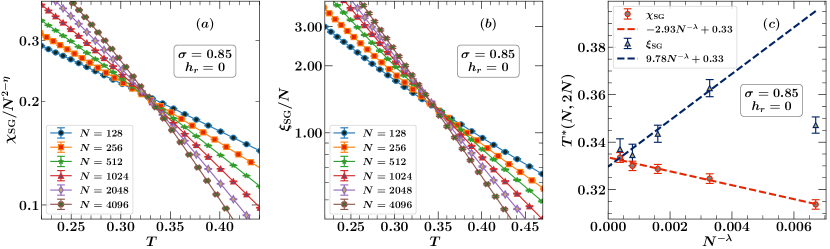
Figure 6: A finite size scaling plot of $\chi_{\text{SG}}$ (figure (a)) and $\xi_{\text{SG}}$ (figure (b)), for $\sigma=0.85$ in the absence of magnetic field ($h_{r}=0$) (with $2-\eta=2\sigma-1$). Both the datasets clearly indicate that a phase transition occurs. The transition temperature in the thermodynamic limit is estimated in figure (c). A non-linear fit of the $\chi_{\text{SG}}$ data from figure (c) with the Eq. (17) using the Levenberg-Marquadt algorithm gives $\lambda=1.03$ (see Table 1). A linear fit of the data using this value of $\lambda$ gives $T_{c}=0.3336\pm 0.0013$ from $\chi_{\text{SG}}$ and $T_{c}=0.3297\pm 0.0036$ from $\xi_{\text{SG}}$.

V Analyses of the simulation data assuming there is an AT line

We shall study the phase transitions at $h_{r}=0$, and determine the zero-field transition temperature $T_{c}$ ($=T_{\text{AT}}(h_{r}=0)$), and seek evidence of an AT transition at non-zero $h_{r}$ using the standard critical point finite size scaling method of determining the “crossings” or intersections of the curves of, say, $\chi_{\text{SG}}/N^{z}$ (with $z=1/3$ when $\sigma\leq 2/3$, and with $z=2-\eta=2\sigma-1$ for $\sigma\geq 2/3$) at values of $N$ and $2N$ as we reduce $T$ through the AT transition temperature at fixed $h_{r}$, or the field $h_{r}$ at fixed $T$ in the vicinity of the AT field $h_{\text{AT}}(T)$ as outlined in Sec. IV. There seems no reason to doubt the existence of an AT line for any value of $\sigma$ in the mean-field region $\sigma<2/3$, and our results are entirely consistent with the existence of an AT transition at $\sigma=0.60$. They serve as a useful comparison for the studies in the non-mean-field regime $\sigma>2/3$, where the evidence will be found to favor the droplet picture. We have studied $N$ values 128, 256, 512, 1024, 2048, 4096, 8192 and 16384 for both $\sigma=0.60$ and $\sigma=0.75$, but went up to $N=32768$ for the case of $\sigma=0.75$ when the field $h_{r}$ was varied at fixed $T$. When $\sigma=0.85$ the largest $N$ values used was $4096$. In this case the zero-field transition temperature $T_{c}$ is quite low and as a consequence all the investigations have to be done also at low temperatures, where equilibration times are long, preventing the study of larger systems. We are mainly interested in the question as to whether outside the mean-field region, that is for $\sigma>2/3$, an AT transition actually exists and whether (say) the dependence of $\xi_{\text{SG}}$ on the field $h_{r}$ can be understood as will be suggested in Sec. VI on the droplet picture without invoking an AT transition at all. If it can, this would provide support to the argument that the droplet scaling picture rather than replica symmetry breaking describes spin glasses below $6$ dimensions. We have analysed the data for $\sigma=0.70,\,\,0.75$ and for $\sigma=0.85$ using the usual “crossing” method, (the finite size scaling approach outlined in Sec. IV), which indeed works well for $\sigma=0.6$. The evidence for the existence of an AT transition at $\sigma=0.75$ and $0.85$ will be contrasted with the evidence against an AT transition at these values of $\sigma$.

Our main focus was the case $\sigma=0.75$. We looked briefly at the case $\sigma=0.70$ to find whether or not it might be practical to study whether $\sigma=2/3$ is the value of $\sigma$ above which the AT line might disappear. We found that it was similar to $\sigma=0.75$, but that the corrections to scaling were larger. This means that for a given level of accuracy, larger $N$ values are required. We studied $\sigma=0.85$ because it should behave similarly to physical systems in three dimensions but we could not equilibrate systems at the larger $N$ values in this case because the temperatures $T$ of interest have to be less than $T_{c}$, which is rather small.

V.1 $\sigma=0.6$

Figure 7: Finite size scaling plots for $\sigma=0.85$ are shown: (a) for $\chi_{\text{SG}}$ with $h_{r}=0.05$, (b) for $\xi_{\text{SG}}$ with $h_{r}=0.05$, (c) for $\chi_{\text{SG}}$ with $h_{r}=0.02$, and (d) for $\xi_{\text{SG}}$ with $h_{r}=0.02$. Figure (c) shows that the data do not intersect even at very low temperatures (much lower than the mean field value of $T_{\text{AT}}(h_{r}=0.02)=0.2997$ obtained using Eq. (8)) indicating that there is no phase transition in this regime. In figures (b) and (d), the data show merging behavior at low temperatures.

We shall focus on $\sigma=0.60$ in this subsection. It corresponds according to Eq. (9) to an effective dimension of $10$ dimensions, which is in the mean-field region; it lies above the upper critical dimension of spin glasses, which is $6$ (or in the mean-field region $\sigma<2/3$ in the one-dimensional long-range model). It is natural to expect that for this value of $\sigma$ there will be an AT line and this is amply confirmed by our simulations. For this value of $\sigma$, simulations of the corresponding Ising model [12, 15] and the Heisenberg model [18, 17] also found an AT line.

Our results for $h_{r}=0$ are given in Figs. 2(a), 2(b), and 2(c). According to Eq. (14b), the data for $\chi_{\text{SG}}/N^{1/3}$ when plotted for different system sizes should intersect at the transition temperature $T_{c}$. Similarly, according to Eq. (19b), the data of $\xi_{\text{SG}}/N^{d_{\text{eff}}/6}$ with $d_{\text{eff}}=2/(2\sigma-1)$ should intersect at the same transition temperature. Figs. 2(a) and 2(b) show the data for different system sizes. We find the temperature $T^{*}(N,2N)$ at which the curves corresponding to the system sizes $N$ and $2N$ intersect. We then fit this data with Eq. (17) to find the transition temperature. The exponent $\lambda\equiv 5/3-2\sigma$ is known to equal $0.467$ in this case  [17, 39]. The result is displayed in Fig. 2(c), where the $T^{*}(N,2N)$ data obtained from intersections of $\chi_{\text{SG}}$ are fitted against $N^{-\lambda}$ with a straight line for the largest $6$ pairs of system sizes to give $T_{c}=0.8873\pm 0.0017$. The corresponding intersections of the $\xi_{\text{SG}}$ data (omitting the two smallest system sizes) gives $T_{c}=0.8893\pm 0.0046$. The values of $T_{c}$ obtained from $\chi_{\text{SG}}$ data and $\xi_{\text{SG}}$ data are in agreement with each other. The mean-field prediction of Eq. (7) is much higher, $T_{c}^{\text{MF}}=\sqrt{6}/2=1.2247$. Fluctuation effects not present in the SK limit must be responsible for this large difference.

For $h_{r}=0.1$, the data is as shown in Figs. 2(d), 2(e), and 2(f). When the $T^{*}(N,2N)$ data obtained from $\chi_{\text{SG}}$ are fitted against $N^{-\lambda}$ with a straight line for the largest $4$ pairs of system sizes we get $T_{\text{AT}}(h_{r}=0.1)=0.6735\pm 0.0120$. The corresponding $\xi_{\text{SG}}$ data (omitting the two smallest system sizes) gives $T_{\text{AT}}(h_{r}=0.1)=0.6745\pm 0.0148$.

Thus we have found that the AT line passes through the point $(T,h_{r})=(0.674,0.1)$. To compare that with the predictions from the SK model, we use the zero-field transition temperature $T_{c}=0.887$ obtained above. Then for $h_{r}=0.1$, the predicted value of the AT transition temperature ratio of the SK model (from Eq. 8) would be $T_{\text{AT}}(h_{r}=0.1)/T_{c}=0.74$, while the Monte Carlo determined value at $\sigma=0.6$ is $0.7590\pm 0.0113$. (For the SK model, the Monte Carlo value of the ratio is $0.7641\pm 0.0341$). Thus while the zero-field transition temperature at $\sigma=0.6$ is not close to the mean-field value of Eq. (7), the SK form of the AT line is a good approximation provided it is expressed in terms of the renormalized zero-field transition temperature $T_{c}$ (see also Fig. 1).

The AT line can be approached not only by reducing the temperature $T$ but also by reducing the field at fixed $T$. In Figs. 3(a) and 3(b) we have constructed the crossing plots at fixed temperature $T=0.6$ $(=0.67\,T_{c})$ as a function of $h_{r}$ for $\chi_{\text{SG}}$ and $\xi_{\text{SG}}$ respectively. Analysis of the crossing plots of $h^{*}(N,2N)$ in Fig. 3(c) shows that the behavior is again consistent with the existence of an AT line at least at $\sigma=0.60$. The same value of $\lambda$ was used as when plotting $T^{*}(N,2N)$. The $h^{*}(N,2N)$ data for all the pairs of system sizes are fitted against $N^{-\lambda}$ to give $h_{\text{AT}}(T=0.6)=0.1569\pm 0.0061$ from $\chi_{\text{SG}}$ and $h_{\text{AT}}(T=0.6)=0.1571\pm 0.0067$ from $\xi_{\text{SG}}$. We found two points on the AT line, $(T,h_{r})=(0.674,0.1)$ from $T^{*}(N,2N)$, and $(T,h_{r})=(0.6,0.157)$ from $h^{*}(N,2N)$ data. These points are plotted in Fig. 1 for comparison with the exact AT line for the SK model.

V.2 $\sigma=0.75$

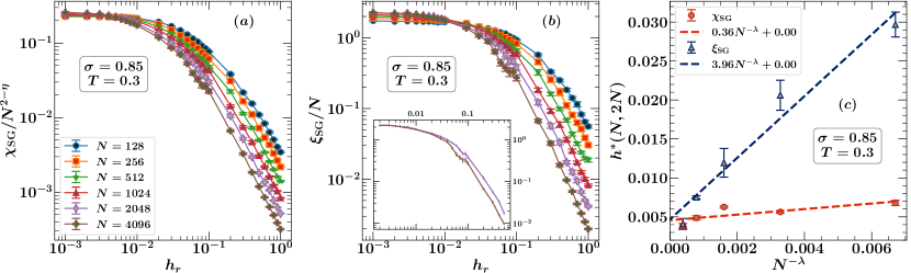
Figure 8: Finite size scaling plots of (a) $\chi_{\text{SG}}$ and (b) $\xi_{\text{SG}}$ as a function of magnetic field $h_{r}$, for $\sigma=0.85$ at a temperature of $T=0.3$ $(=0.91\,T_{c})$. The inset of figure (b) shows the data for the two largest system sizes $N=2048$ and $N=4096$. The common legend for both the figures (a) and (b) is shown in figure (a). The intersection fields $h^{*}(N,2N)$ data is shown in figure (c). We substitue the value of the exponent $\lambda=1.03$ (see Table 1) obtained from the $T^{*}(N,2N)$ data at $h_{r}=0$ in Eq. (22) and fit $h^{*}(N,2N)$ data agianst $N^{-\lambda}$ to get $h_{\text{AT}}(T=0.3)=0.0046\pm 0.0006$ from $\chi_{\text{SG}}$ and $h_{\text{AT}}(T=0.3)=0.0047\pm 0.0016$ from $\xi_{\text{SG}}$.

The case $\sigma=0.75$ corresponds to the non-mean-field regime: the long-range diluted model for this value of $\sigma$ is equivalent to a short-range model with $d\approx 4$ dimensions. In this regime, simulations of the corresponding Heisenberg model [18, 17] were thought consistent with an AT transition.

According to Eq. (14a), the data for $\chi_{\text{SG}}/N^{2-\eta}$,where $2-\eta=2\sigma-1$, plotted for different system sizes should intersect at the transition temperature $T_{c}$. Similarly, according to Eq. (19a), the curves of $\xi_{\text{SG}}/N$ should also intersect at the transition temperature. Figs. 4(a) and 4(d) show the finite-size-scaled data of $\chi_{\text{SG}}$, and Figs. 4(b) and 4(e) show the finite-size-scaled data of $\xi_{\text{SG}}$. The curves for different system sizes show a clear tendency to intersect close to the same temperature. The data for $T^{*}(N,2N)$ are then fitted with Eq. (17) where the value of the exponent $\lambda$ is not known in the non-mean-field regime and hence should be considered as a fitting parameter.

If there were an AT transition there would be a unique value of $\lambda$, the same for both the $\xi_{\text{SG}}$ and $\chi_{\text{SG}}$ intersections corresponding to both $h^{*}(N,2N)$ and $T^{*}(N,2N)$. In order to find the value of $\lambda$ through non-linear fitting, we have six different sets of data: $T^{*}(N,2N)$ obtained from $\chi_{\text{SG}}$ and $\xi_{\text{SG}}$ intersections, with $h_{r}=0$ and $h_{r}=0.05$ (Figs. 4(a), 4(b), 4(d), and 4(e)), and $h^{*}(N,2N)$ obtained from $\chi_{\text{SG}}$ and $\xi_{\text{SG}}$ intersections at $T=0.55$ (Figs. 5(a) and 5(b)). We tried fitting these individual data sets with Eq. (17) (Eq. (22) for $h^{*}(N,2N)$) through non-linear fitting by considering $\lambda$, $T_{c}$ and $A$ ($\tilde{A}$ for $h^{*}(N,2N)$) as fitting parameters. This is a non-linear fitting procedure for which we use efficient methods like the Trusted Region Reflective (TRF) algorithm and the Levenberg-Marquardt (LM) algorithm (for which packages are available in python) to determine the fitting parameters. Doing so, we found that the $h^{*}(N,2N)$ data obtained from the $\chi_{\text{SG}}$ intersections at $T=0.55$ (Fig. 5(a)) gave us the best fit (using chi-square test), and we obtain $\lambda=0.26$ (see Table 1). Since the exponent giving the leading correction to scaling $\lambda$ is universal, we use the same value of $\lambda$ with both intersections $h^{*}(N,2N)$ and $T^{*}(N,2N)$ obtained from $\chi_{\text{SG}}$ and $\xi_{\text{SG}}$ data. We substitute the value of $\lambda$ obtained above in Eq. (17) and fit the $T^{*}(N,2N)$ data against $N^{-\lambda}$ with a straight line. As shown in Fig. 4(c), for $h_{r}=0$, the $\chi_{\text{SG}}$ fit (considering all the pairs of system sizes) gives $T_{c}=0.6200\pm 0.0031$. The corresponding $\xi_{\text{SG}}$ fit (omitting the smallest system size) gives $T_{c}=0.6244\pm 0.0098$.

For $h_{r}=0.05$, the intersection temperatures data are shown in Fig. 4(f). Omitting the smallest system size, the $T^{*}(N,2N)$ data are fitted with Eq. (17) to give $T_{\text{AT}}(h_{r}=0.05)=0.4395\pm 0.0241$ from $\chi_{\text{SG}}$ and $T_{\text{AT}}(h_{r}=0.05)=0.2893\,\pm\,0.0252$ from $\xi_{\text{SG}}$. Compared to Fig. 2(f) which gives the equivalent plot for the case with $\sigma=0.60$, the data in Fig. 4(f) does not look like data which is converging to the same asymptotic limit when $N$ is large. If the crossings were actually due to a genuine AT transition, then the asymptotic limit should be the same for both. If we follow the mean-field prescription (Eq. 8) that is applicable to the SK model, the spin glass transition temperature for $h_{r}=0.05$ is $T_{\text{AT}}(h_{r}=0.05)/T_{c}=0.83$. The minimum temperature we simulated for $\sigma=0.75$ is $T_{\text{min}}/T_{c}=0.45$ (look at Table 3), which is $0.54$ times the mean-field prediction. On the other hand, for $\sigma=0.60$ with $h_{r}=0.1$, the mean-field calculations give $T_{\text{AT}}(h_{r}=0.1)/T_{c}=0.74$, and the minimum temperature simulated for this case is $T_{\text{min}}/T_{c}=0.56$. So, for $\sigma=0.60$ the minimum temperature simulated is just $76\%$ of the mean-field transition temperature at that particular field and still we were able to observe clear signs of a phase transition. In contrast, for $\sigma=0.75$, we went down to a much lower temperature which is $54\%$ of the mean-field spin glass transition temperature at $h_{r}=0.05$ and still we couldn’t see clear signs of a phase transition.

We have also studied $\chi_{\text{SG}}$ and $\xi_{\text{SG}}$ at fixed $T$, but varying $h_{r}$ and the finite size scaling plots for these are given in Figs. 5(a) and 5(b). There appears to be good intersections in the curves, supporting therefore the possible existence of an AT transition at the temperature studied $T=0.55$ $(=0.89\,T_{c})$. A plot of $h^{*}(N,2N)$ versus $1/N^{\lambda}$ is in Fig. 5(c), using the same value of $\lambda=0.26$. In the intersections of $\xi_{\text{SG}}$ there is a clear rising trend of $h^{*}(N,2N)$ with increasing $N$ until $N=1024$, followed by decreasing values of $h^{*}(N,2N)$ for $N>2048$. For the case of $\sigma=0.60$, where there is almost certainly a genuine AT transition, (Fig. 3(c)) only the rising trend is seen. It is as if for the smaller systems $N<2048$ the system at $\sigma=0.75$ is behaving similarly to its mean-field cousin at $\sigma=0.60$. Note that this change of trend cannot be attributed to the correction to scaling terms of Eq. (23). These only apply in the limit $N\to\infty$ with $N^{1/\nu}(h_{r}-h_{\text{AT}}(T))$ fixed. For a genuine AT transition the intersections $h^{*}(N,2N)$ from both $\xi_{\text{SG}}$ and $\chi_{\text{SG}}$ should both extrapolate as $N\to\infty$ to the same field $h_{\text{AT}}(T)$. It is hard to argue that Fig. 5(c) provides good evidence for this. On the other hand, on the droplet picture, it would be expected that $h^{*}(N,2N)$ should extrapolate to zero. The evidence that is happening is also weak.

V.3 $\sigma=0.85$

Figure 9: Figures in the top row show $\chi_{\text{SG}}$ plotted as a function of magnetic field $h_{r}$ at fixed temperature, for: (a) $\sigma=0.6$ at $T=0.6$, (b) $\sigma=0.75$ at $T=0.55$, and (c) $\sigma=0.85$ at $T=0.3$. Figures in the bottom row show plots of $\xi_{\text{SG}}$ versus $h_{r}$ for: (d) $\sigma=0.6$ at $T=0.6$, (e) $\sigma=0.75$ at $T=0.55$, and (f) $\sigma=0.85$ at $T=0.3$. For large values of $h_{r}$, we fitted the $\chi_{\text{SG}}$ data with $1/h_{r}^{x_{\chi}}$ and $\xi_{\text{SG}}$ data with $1/h_{r}^{x}$. The color labelling for different system sizes is same for all these figures, and the common legend is displayed at the top. The values of exponents $x_{\chi}$, $x$, and $z=x_{\chi}/x$ obtained from curve fitting are presented in Table 2.

Table 1: Values of the exponent $\lambda$ obtained from our simulations for different values of $\sigma$. The last column shows the values of $\chi^{2}/N_{\text{dof}}$ which is a measure of goodness-of-fit. $N_{\text{dof}}$ denotes the number of degrees of freedom. For $\sigma=0.75$, the value of $\lambda$ shown here is obtained by fitting the $h^{*}(N,2N)$ data obtained from $\chi_{\text{SG}}$ intersections in Fig. 5(a) with Eq. (22) using efficient non-linear fitting algorithms. For $\sigma=0.85$, we use the $T^{*}(N,2N)$ data from $\chi_{\text{SG}}$ intersections in Fig. 6(a) to determine $\lambda$. For convenience, we include a column showing our estimates for the zero-field spin glass transition temperature for different $\sigma$. These values are obtained from the fits shown in Figs. 2(c), 4(c), and 6(c).

$\sigma$	$T_{c}$	$\lambda$	$\chi^{2}/N_{\text{dof}}$
$0.60$	$0.89$	$0.47$	-
$0.75$	$0.62$	$0.26$	$1.03$
$0.85$	$0.33$	$1.03$	$0.39$

For $\sigma=0.85$ we are further into the non-mean-field region. According to Eq. (9), $\sigma=0.85$ corresponds to a short-range model close to three dimensions. In this regime, simulations of the corresponding Heisenberg model [18, 17] did not find an AT line.

For $h_{r}=0$, Figs. 6(a) and 6(b) clearly show that the curves for different system sizes are intersecting. The data for intersection temperatures are shown in Fig. 6(c). Similar to the case of $\sigma=0.75$, the $T^{*}(N,2N)$ data obtained from $\chi_{\text{SG}}$ and $\xi_{\text{SG}}$ intersections with $h_{r}=0$ (Figs. 6(a) and 6(b)), and the $h^{*}(N,2N)$ obtained from $\chi_{\text{SG}}$ and $\xi_{\text{SG}}$ intersections at $T=0.3$ (Figs. 8(a) and 8(b)) are fitted with Eq. (17) (Eq. (22) for $h^{*}(N,2N)$) by considering $\lambda$, $T_{c}$, and $A$ ($\tilde{A}$ for $h^{*}(N,2N)$) as fitting parameters, and found that the $T^{*}(N,2N)$ data obtained from the $\chi_{\text{SG}}$ intersections gave us the best fit. We obtain $\lambda=1.03$ (see Table 1) from both TRF and LM methods. We use this value of $\lambda$ in Eqs. (17) and (22) for further calculations. The fit using the $\chi_{\text{SG}}$ data for all the pairs of system sizes gives $T_{c}=0.3336\pm 0.0013$. The corresponding $\xi_{\text{SG}}$ fit (omitting the smallest system size) gives $T_{c}=0.3297\pm 0.0036$. The two values of $T_{c}$ are quite close.

For $h_{r}=0.05$ the $\chi_{\text{SG}}/N^{2-\eta}$ data do not intersect as shown in Fig. 7(a). Such a field could conceivably be above the largest AT field even at $T=0$, so we also studied a smaller field: $h_{r}=0.02$ shown in Fig. 7(c). There is no sign of any crossing at this field either!. The $\xi_{\text{SG}}$ data is less clearcut. Fig. 7(b) shows there are no intersections at a field of $h_{r}=0.05$ while a merging behavior is seen for the larger systems at $h_{r}=0.02$, as shown in Fig. 7(d). In our simulations we went to very low temperatures such as $T=0.1$, which is small in comparison with the mean-field values of $T_{\text{AT}}$ for $h_{r}=0.02$ and $h_{r}=0.05$ using Eq. (8), but we still could not find any clear intersections in the $\chi_{\text{SG}}$ or $\xi_{\text{SG}}$ data. This suggests that there is no phase transition in this regime in the presence of a magnetic field. Our data are consistent with the scenario where the external magnetic field destroys the phase transition, just as happens for a ferromagnet when a uniform field is turned on. Very similar features were seen for the Heisenberg version of this model [18, 17] and in the three dimensional Ising model [35].

Confusingly, intersections are seen at fixed $T=0.3$ $(=0.91\,T_{c})$ as $h_{r}$ is varied in the plots of $\chi_{\text{SG}}/N^{2-\eta}$ in Fig. 8(a) and of $\xi_{\text{SG}}/N$ in Fig. 8(b). The usual analysis of $h^{*}(N,2N)$ is given in Fig. 8(c). Thus in crossing the AT line along a trajectory of fixed $T$ we have seen intersections, suggesting there might be an AT transition. However, the large $N$ limit of $h^{*}(N,2N)$ in Fig. 8(c) in the case of $\sigma=0.85$, suggests that $h_{\text{AT}}(T)$ might actually be zero, consistent with the droplet scaling picture. In the next section the dependence of $\xi_{\text{SG}}$ and $\chi_{\text{SG}}$ on $h_{r}$ will be explained using the droplet scaling approach.

VI Data analyses on the droplet picture

Figure 10: Finite size scaling analysis of $\chi_{\text{SG}}$ data (figures (a),(b),(c)) and $\xi_{\text{SG}}$ data (figures (d),(e),(f)) on the droplet picture, obtained by fixing the temperature $T$ and varying the magnetic field $h_{r}$. The data are plotted on a log-log scale. Figures (a) and (d) are for $\sigma=0.6$ at $T=0.6$, (b) and (e) are for $\sigma=0.75$ at $T=0.55$, and (c) and (f) are for $\sigma=0.85$ at $T=0.3$. The corresponding inset figures show our data for the two largest system sizes: $N=8192\text{ and }16384$ for $\sigma=0.6$, $N=16384\text{ and }32768$ for $\sigma=0.75$, and $N=2048\text{ and }4096$ for $\sigma=0.85$. The legend displayed at the top is common for all the figures (both main and inset). The values of the exponents $x$ and $z$ are given in Table 2.

In this section we give the field dependence of $\xi_{\text{SG}}$ and $\chi_{\text{SG}}$ according to the droplet picture [45, 46, 47], including also their finite size modifications, and compare these with our simulation data.

In the droplet picture one uses an Imry-Ma argument [48] for the correlation length $\xi$ and identifies it with the size of the region or domain within which the spins become re-oriented in the presence of the random field. The free energy gained from such a reorientation by the the random field is of order $\sqrt{q_{\text{EA}}(T)}h_{r}\xi^{d/2}$. The size of such domains $\xi$ is determined by equating this free energy to the free energy cost of the interface of this domain of re-ordered spins with the rest of the system, which is of the form $\Upsilon(T)\xi^{\theta}$  [49]. Equating these two free energies gives

$$\xi\sim\bigg{[}\frac{\Upsilon(T)}{\sqrt{q_{\text{EA}}(T)}h_{r}}\bigg{]}^{1/(d/2-\theta)}.$$ (24)

While there is a considerable literature on the dependence of the interface exponent $\theta$ on $\sigma$ for the case of Ising spin glasses  [50], we know of no equivalent studies for the case of the XY spin glass. (Our data suggests that its $\theta$ might be close to that of the Ising spin glass).

Eq. (24) shows that as $h_{r}\to 0$, the length scale becomes infinite; $\xi$ diverges as $\xi\sim 1/h_{r}^{x}$, where

$$x=\frac{1}{d/2-\theta}.$$ (25)

The exponent $x$ is the analogue of $\nu$ at the AT transition; it is as if the AT transition $h_{\text{AT}}(T)=0$. We would expect this formula to apply until finite size effects limit its growth, which will occur when $\xi$ is of $O(L)$ (or $O(N)$ in our one-dimensional system). Identifying $\xi_{\text{SG}}$ with $\xi$, Figs. 9(e) and 9(f) show that the Imry-Ma fit indeed works well at the larger fields; the data for the larger $h_{r}$ collapse nicely onto a power law form as predicted by Eq. (24) for all sizes $N$. It only departs from this formula when $\xi_{\text{SG}}$ becomes of order $N$, when finite size corrections to the Imry-Ma formula are needed. Also TNT effects (see Sec. VII) produce corrections to the Imry-Ma formula when $\xi_{\text{SG}}$ is of $O(N)$ unless $N=L>L^{*}$. The crossover scale $L^{*}$ is thought to be large, especially as $\sigma$ approaches $2/3$ (or $d\to 6$) [3].

To allow for finite size effects on the Imry-Ma formula we use the analogue of Eq. (21a) with $h_{\text{AT}}=0$ and $\nu=x$ to write:

$$\frac{\xi_{\text{SG}}}{N}=\mathcal{X}(N^{1/x}h_{r}).$$ (26)

Our results for $\sigma=0.75$ are shown in Fig. 10(e) and for $\sigma=0.85$ are shown in Fig.  10(f). There are clearly finite size corrections to this formula. It is a formula which formally would be expected to hold in the scaling limit of $N\to\infty$ with $N^{1/x}h_{r}$ fixed. The crossover function $\mathcal{X}(y)\sim 1/y^{x}$ when $y$ is large, in order to recover Eq. (24). It goes to a constant when $y\to 0$. However, a closer look at our two largest system sizes $N=16384$ and $N=32768$ at $\sigma=0.75$ (inset to Fig. 10(e)) and our two largest system sizes at $\sigma=0.85$, $N=2048$ and $N=4096$ (inset to Fig. 10(f)) shows that the finite size corrections are becoming small, and are smaller the further the system is away from the mean-field region. If one moves in the other direction, towards the start of the mean-field region $\sigma=2/3$, the finite size corrections are larger, as seen in Fig. 13(b) for $\sigma=0.70$. The finite size scaling form for these corrections to the scaling of Eq. (26) will be of the form

$$\frac{\xi_{\text{SG}}}{N}=\mathcal{X}(N^{1/x}h_{r})+N^{-\omega}\mathcal{H}(N^{1/x}h_{r}),$$ (27)

where $\omega$ is the correction to scaling exponent. However, TNT effects (see Sec. VII) produce large further corrections to these asymptotic forms when $L<L^{*}$. Since in our studies $L^{*}$ is probably larger than the length $N$ of our system, at least for $\sigma=0.75$, the scaling form of Eq. (27) does not work in the region where $\xi_{\text{SG}}$ is of order $N$ (see Fig. 14(a)). For $\sigma=0.85$ where $L^{*}$ is expected to be smaller, Fig. 14(b) hints that Eq. (27) might apply as the plots at adjacent sizes for the larger $N$ values seem to be getting closer together as $N$ is increased, which is a feature predicted by Eq. (27).

In Fig. 9(d) we show a similar plot to those in Figs. 9(e) and 9(f) but for the case of $\sigma=0.60$. Notice however that because of the AT transition at this value of $\sigma$, at which $\xi_{\text{SG}}$ would diverge to infinity as $N\to\infty$ at some finite field $h_{r}=h_{\text{AT}}(T)$, a shoulder above the dashed line has started to appear which is the beginning of this divergence. Such a feature is absent in the figures for both $\sigma=0.75$ and at $\sigma=0.85$. Similarly, Fig. 10(d) shows poor collapse of $\xi_{\text{SG}}$ data for $\sigma=0.6$, which is in contrast to the cases of $\sigma=0.75$ and $\sigma=0.85$. This indicates that the $\xi_{\text{SG}}$ data for $\sigma=0.6$ is not in accordance with Eq. 27.

Figure 11: A plot of $h^{*}(N,2N)N^{1/x}$ versus $1/N^{\omega}$, for $\sigma=0.70,0.75$ and $0.85$. The values of $x$ and $\omega$, which is obtained from Eq. (36) were taken from Table 2.

The spin glass susceptibility according to the droplet picture is a similar generalization of the finite size scaling form of Eq. (14a):

$$\frac{\chi_{\text{SG}}}{N^{z}}=\mathcal{C}(N^{1/x}h_{r}),\quad(2/3\leq\sigma<1).$$ (28)

The crossover function $\mathcal{C}(y)\sim 1/y^{x_{\chi}}$ when $y$ is large, so that then $\chi_{\text{SG}}\sim\xi^{z}$ and becomes independent of $N$. Its form is then

$$\chi_{\text{SG}}\sim 1/h_{r}^{x_{\chi}},$$ (29)

which implies that $x_{\chi}=xz$. In the opposite limit as $y\to 0$, $C(y)$ goes to a finite constant. Figs. 9(a), 9(b), and 9(c) show that the $\chi_{\text{SG}}$ data for the larger $h_{r}$ collapse nicely onto a power law form as predicted by Eq. (29) for all sizes $N$. The exponent $z$ depends upon whether we are dealing with short-range interactions, (such as nearest-neighbor interactions) or with the long-range interactions employed in this paper. For short-range interactions, the average value of $\chi_{ij}^{2}$ falls off with spin separation $r_{ij}$ as

$$\overline{\chi_{ij}^{2}}\sim\frac{\left(q_{\text{EA}}(T)\right)^{2}T}{\Upsilon(T)r_{ij}^{\theta}},$$ (30)

[46, 47]. This result applies in the zero-field spin glass state. Then as,

$$\chi_{\text{SG}}=\frac{1}{N}\sum_{i,j=1}^{N}\overline{\chi_{ij}^{2}},$$ (31)

so in $d$ dimensions for the zero-field spin glass $\chi_{\text{SG}}\sim L^{d-\theta}$. Hence

$$z=\frac{d-\theta}{d},$$ (32)

in order to recover the result $\chi_{\text{SG}}\to N^{z}$ as $N^{1/x}h_{r}$ goes to zero. We caution that this formula for $z$ will only hold for short-range interactions.

With long-range interactions a “droplet” is not a single connected region but a set of isolated islands of flipped spins [50] and this will make the decay of $\chi_{ij}^{2}$ with $r_{ij}$ faster than in Eq. (30). This is an effect which has not been studied before, and so in our problem the exponent $z$ has to be determined by fitting the data. The results of our determinations of the droplet exponents $x$, $x_{\chi}$ and $z$ for the different values of $\sigma$ which we have studied are summarised in Table 2.

The resulting excellent data collapse (at least when $\xi_{\text{SG}}<N$), is shown in Figs. 10(b) and 10(c). The value of $z$ was determined from the observation that when $N^{1/x}h_{r}$ is large, $\chi_{\text{SG}}$ should be independent of $N$. It is remarkable that $z$ determined at large values of $N^{1/x}h_{r}$ results in a decent collapse of the data in the opposite limit where $N^{1/x}h_{r}\to 0$. Nevertheless corrections to the Imry-Ma scaling form are visible in the figures (and are sizeable in the region where $N^{1/x}h_{r}$ is small when viewed in a linear plot rather than a log scale plot, (just as in the $\xi_{\text{SG}}$ plots Figs. 10(e) and 10(f)). In the limit when $N^{1/x}h_{r}$ is held fixed with $N\to\infty$ the leading correction to scaling will be

$$\frac{\chi_{\text{SG}}}{N^{z}}=\mathcal{C}(N^{1/x}h_{r})+N^{-\omega}\mathcal{G}(N^{1/x}h_{r}),$$ (33)

where $\mathcal{G}(y)$ is an unknown scaling function and the correction to scaling exponent $\omega$ is not known with any certainty (but see Eq. (36)).

Table 2: Values of the exponents $x_{\chi}$, $x$, and $z$ obtained from our simulations for different values of $\sigma$ and $T$ (look at Fig. 9).

$\sigma$	$T$	$x_{\chi}$	$x$	$z$
$0.7$	$0.6$	$1.5747\pm 0.0009$	$3.3220\pm 0.0413$	$0.4740\pm 0.0062$
$0.75$	$0.55$	$1.6114\pm 0.0005$	$2.7077\pm 0.0531$	$0.5951\pm 0.0119$
$0.85$	$0.3$	$1.8919\pm 0.0014$	$2.2019\pm 0.0152$	$0.8592\pm 0.0066$

Figure 12: A plot of $R$ (Eq. (35)) versus $N$, obtained from the data generated by varying the magnetic field $h_{r}$ at a fixed temperature $T$. The data is shown for: (a) $\sigma=0.6$ at $T=0.6$, (b) $\sigma=0.75$ at $T=0.55$, and (c) $\sigma=0.85$ at $T=0.3$. The quantity $R$ is the y-coordinate of the point where the curves for adjacent sizes in Figs. 3(a), 5(a), and 8(a) intersect.

Let us suppose that the droplet picture is correct and that (say) the spin glass susceptibility $\chi_{\text{SG}}$ is described by Eq. (28). This equation predicts that there will be a crossing in the plots of $\chi_{\text{SG}}/N^{2\sigma-1}$ used in AT line critical scaling studies. (Note we are setting $2-\eta=2\sigma-1$). The correction to scaling term of Eq. (33) is not needed for this, but this correction does strongly influence where the crossings take place for the $N$ values which are reached in our simulations. The crossing arises as follows. At small values of $h_{r}N^{1/x}$, the function $\mathcal{C}$ goes to a constant. It turns out that $z>(2\sigma-1)$, so $\chi_{\text{SG}}/N^{2\sigma-1}$ diverges as $N$ is increased as $N^{z-(2\sigma-1)}$ as $h_{r}\to 0$. On the other hand when $h_{r}N^{1/x}$ is large, $\chi_{\text{SG}}\to 1/h_{r}^{z}$, so $\chi_{\text{SG}}/N^{2\sigma-1}\to 1/N^{2\sigma-1}h_{r}^{z}\to 0$ as $N$ goes to infinity. Because at small fields, $\chi_{\text{SG}}/N^{2\sigma-1}$ is larger for large $N$, but at bigger $h_{r}$ fields it is smaller at the larger $N$ values, so there must be a crossing point. We shall denote the crossing value between the lines at $N$ and $2N$ by $h^{*}(N,2N)=H$. Then $H$ is determined by the solution of the following

$$\frac{\chi_{\text{SG}}(H,N)}{N^{2\sigma-1}}=\mathcal{C}(N^{1/x}H)N^{z-(2\sigma-1)}=$$

$$\frac{\chi_{\text{SG}}(H,2N)}{(2N)^{2\sigma-1}}=\mathcal{C}((2N)^{1/x}H)(2N)^{z-(2\sigma-1)}.$$ (34)

Assuming $\mathcal{C}(y)\rightarrow a-by$, when $y\to 0$, it is easy to show then that the $N$ dependence of $h^{*}(N,2N)$ at very large $N$ will be as $1/N^{1/x}$. In reality we have no data in this region of very large $N$ where the corrections to scaling term in Eq. (33) can be ignored. The corrections to scaling are numerically small but are very important in determining the values of $h^{*}(N,2N)$.

There is a similar crossing predicted in the plots of $\xi_{\text{SG}}/N$ as a function of $h_{r}$ when Eq. (27) holds, using the analogue of Eq. (34). In this case it is the scaling correction which causes the curves to cross, (which requires $\mathcal{H}(0)$ to be negative), and for these curves the crossings $h^{*}(N,2N)$ at very large $N$ will decrease as $1/N^{1/x+\omega}$, (compare with Eq. (18b)) on taking $\chi(y)=c-dy$ and $\mathcal{H}(y)\to\text{constant}$ as $y\to 0$. Once again we have no data in this very large $N$ regime. In Fig. 11 we have plotted $h^{*}(N,2N)N^{1/x}$ versus $1/N^{\omega}$, assuming that $\omega$ is given by Eq. (36). Note that the size of the corrections to scaling $\sim 1/N^{\omega}$ is simply not small for the values of $N$ which we can study, contrary to what was assumed in the above. $h^{*}(N,2N)N^{1/x}$ should go to a constant as $N$ goes to infinity and it is only for the case of $\sigma=0.85$, where the corrections to scaling are the smallest of the three cases studied, does that look remotely possible. For the case of $\sigma=0.70$ the corrections look to be very large. We conclude that for the values of $\sigma=0.70$ and $\sigma=0.75$, the crossing data on $h^{*}(N,2N)$ is not close to the large $N$ asymptotic form predicted by the droplet picture. But the droplet picture does predict that the existence of such intersections.

If we only had information on the values of the crossing fields $h^{*}(N,2N)$ it would be difficult to really be sure whether the droplet picture or the RSB picture best described the data. The results on $h^{*}(N,2N)$ alone are inconclusive as regards both the AT transition line picture and the droplet picture. While on the droplet picture $h^{*}(N,2N)$ are predicted to go to zero as $N\to\infty$, the values of $h^{*}(N,2N)$ are not convincingly going to zero as $N$ is increased (see Fig. 11). Fortunately, there is another way of distinguishing the two approaches, which does not require us to reach the $N$ values at which $h^{*}(N,2N)$ starts to approach zero. We define

$$R\equiv\begin{cases}\dfrac{\chi_{\text{SG}}(h^{*}(N,2N),N)}{N^{2\sigma-1}},&2/3\leq\sigma<1,\\[11.38092pt] \dfrac{\chi_{\text{SG}}(h^{*}(N,2N),N)}{N^{1/3}},&1/2<\sigma\leq 2/3.\end{cases}$$ (35)

(Because we only determine $\chi_{\text{SG}}(h_{r},N)$ at a finite number of values of $h_{r}$, we use linear interpolation to calculate $\chi_{\text{SG}}(h^{*}(N,2N),N)$ using the $\chi_{\text{SG}}(h_{r},N)$ values at the two determined values of $h_{r}$ which lie on either side of $h^{*}(N,2N)$). On the phase transition picture, $R$ should approach a finite constant as $N\to\infty$. On the droplet picture $R$ should increase as $N^{z-(2\sigma-1)}$ as $N\to\infty$. For $\sigma=0.60$ where an AT line is expected $R$ should go to a constant but at the $N$ values studied it actually still appears to be decreasing (see Fig.  12(a)) and has yet to become constant, presumably due to finite size effects. This indicates that trying to determine whether $\sigma=2/3$ is the exact value at which the crossover to droplet scaling behavior will also be challenging from the side below $2/3$. However, for $\sigma=0.75$, Fig. 12(b) shows that $R$ is clearly increasing with $N$ for large $N$ values. But if we had had only data for system sizes $<2048$ we might have indeed concluded that there was good evidence for an AT transition in that $R$ seemed to be an $N$ independent constant. While at the sizes we can reach $R$ is clearly increasing with $N$ it has yet to reach its asymptotic form of increase as $N^{z-(2\sigma-1)}$. The quantity $R$ also increases with $N$ for $\sigma=0.70$ and $\sigma=0.85$, (see for example Fig. 12(c)).

In order for $\chi_{\text{SG}}$ to match as $\sigma\to 2/3$ from either the mean-field side, (where $z=1/3$) with its value in the non-mean field region, we would expect that $z$ should approach $1/3$ as $\sigma\to 2/3$ from above. At $\sigma=0.85$, $z\approx 0.8409$, at $\sigma=0.75$, $z\approx 0.6065$, while at $\sigma=0.70$, we find $z\approx 0.4737$. Thus it seems quite plausible that $z$ could approach $1/3$ as $\sigma\to 2/3$ from above. Then the combination $z-(2\sigma-1)$ would approach zero in this limit, which means that the divergence of $R$ with $N$ will become harder and harder to see as $\sigma$ approaches $2/3$. We conclude that it will be challenging to do numerical work which shows that the AT line disappears at precisely $\sigma=2/3$. On the mean-field side of $2/3$ the correction to scaling exponent $\omega=1/3-(2\sigma-1)$. It therefore seems natural to expect that on the non-mean field regime

$$\omega=z-(2\sigma-1).$$ (36)

If valid, this would imply that corrections to scaling should be larger at $\sigma=0.70$ than at $\sigma=0.75$, and this is what we observed in Figs. 13(b) and 13(a), in comparison with (inset of) Figs. 10(e) and 10(b).

In the presence of a genuine AT transition, as $h_{r}$ is reduced one would pass through three regions: first the paramagnetic state at larger values of $h_{r}$, then the critical region, then the low-temperature phase with RSB at smaller values of $h_{r}$. The good data collapse for all values of $h_{r}$ using Eq. (26), and Eq. (28) shows that at any finite value of $h_{r}$ there is just one region, the paramagnetic region. Studying “intersections” as in Sec.  V is an attempt to find the critical region. But the intersections at finite values of $h_{r}$ for $\sigma=0.75$ and $\sigma=0.85$ are not signs of a genuine phase transition, but at least in the case of $\chi_{\text{SG}}$ these crossings are also just a consequence of droplet scaling. The behavior of $h^{*}(N,2N)$ as a function of $N$ is greatly complicated by finite size effects and will only become clear at much larger $N$ values than those which we have been able to study.

Because on the droplet picture there is no AT line and so one is always in the paramagnetic phase at any non-zero field (just as in a ferromagnet). However, length scales like $\xi_{\text{SG}}$ become very large as $h_{r}\to 0$ for temperatures $T<T_{c}(h_{r}=0)$. Once they become comparable to the system dimensions $L$ and one is in the regime $h_{r}<h^{*}(N,2N)$, the system will have many of the features which might be associated with being in the broken replica symmetric phase which is envisaged to exist below the AT line. For physical systems in three dimensions the relevant length scale is not the linear dimension of the system $L$, but the linear dimension of a fully equilibrated region. This may explain why both simulations and experiments have failed for many years to resolve the debate.

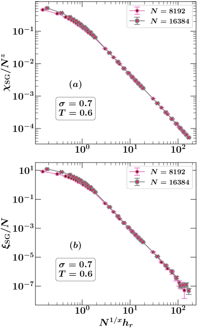
Figure 13: A complete finite size scaling plot of (a) $\chi_{\text{SG}}$ and (b) $\xi_{\text{SG}}$ as a function of magnetic field $h_{r}$, for $\sigma=0.70$ at a temperature of $T=0.6$ $(=0.83\,T_{c},\,T_{c}=0.72)$ for our two largest system sizes.

Might it be possible to find by simulations whether the borderline between RSB ordering and droplet ordering is at $\sigma=2/3$, which is the equivalent of $d=6$ with short-range interactions? To this end we looked at the case of $\sigma=0.70$. We found from studying the crossings of $\xi_{\text{SG}}$ and $\chi_{\text{SG}}$ for the zero field case that the zero field transition temperature is $\approx 0.724$. Figs. 13(a) and 13(b) show our attempt to collapse the data with the droplet scaling forms. Clearly the effects of corrections to scaling are larger than was the case at $\sigma=0.75$ in Figs. 10(e) and 10(b). This is in accord with Eq. (36) which predicts that the correction to scaling exponent $\omega$ will go to zero as $\sigma\to 2/3$ if also $z\to 1/3$ as expected. We conclude that it will be difficult to provide good numerical evidence that $\sigma=2/3$ is the lower critical dimension of the AT transition.

VII TNT versus The Droplet Scaling Picture

Newman and Stein [51] (see also the recent review [52]),have suggested that the ordered phase of spin glasses in finite dimensions will fall into one of 4 categories, (and which one might depend on the dimensionality $d$ of the system): The RSB state is one of these, and is somewhat similar to that envisaged by Parisi for the SK model, but there is also the chaotic pairs state picture of Newman and Stein. In both of these pictures there is an AT transition. The other two pictures are the so-called TNT picture of Krzakala and Martin [36] and Palassini and Young [37] and the droplet scaling picture [45, 46, 47]. In neither the TNT picture nor the droplet scaling picture is there an AT transition. In the droplet picture the Parisi overlap function $P(q)$ is trivial, consisting of two delta functions at $\pm q_{\text{EA}}$ in zero field, whereas in the TNT picture the form of $P(q)$ is quite similar to the non-trivial (NT) form which Parisi found for the SK model. The TNT picture accounts for the non-trivial form of the Parisi overlap function by postulating that there exist droplets of the linear size $L$ of the system, which contain $O(L^{d})$ spins, and which do not have a free energy of order $L^{\theta}$ (as they would in the droplet scaling picture), but which have instead a free energy of $O(1)$. It is the presence of such droplets which makes $P(q)$ non-trivial, which is a feature observed in all simulations of it to date.

In a recent paper [3] one of us argued that once the linear dimension of the system became larger than a crossover length $L^{*}$ the non-trivial behavior observed in $P(q)$ will change to the trivial form predicted by droplet scaling. Estimates of $L^{*}$ in $d=3$ suggest it might be large, of the order of several hundred lattice spacings and it is probably the case that to date the regime where $L>L^{*}$ has not been reached. Furthermore it was suggested that as $d\to 6$, $L^{*}$ would grow towards infinity, as the droplets of $O(1)$ evolve to the $O(1)$ excitations in the Parisi RSB solution, where the pure states have free energies which differ from each other by $O(1)$. In our one dimensional proxy system we would therefore expect to find that $L^{*}$ is much larger when $\sigma=0.75$ than it is when $\sigma=0.85$.

In this paper there are TNT-like effects visible in the behavior of $\xi_{\text{SG}}/N$ in the region where $\xi_{\text{SG}}$ is of $O(N)$ (see Figs. 10(e) and 10(f)). When $\xi_{\text{SG}}$ is of order $N$ the droplets which are important are those of size $N$ and if $L<L^{*}$ some of these will have free energy of $O(1)$ rather than $L^{\theta}$. As a consequence the good scaling collapse of the data visible when $\xi_{\text{SG}}/N\ll 1$ will be lost. In Figs. 14(a) and 14(b) we have plotted $\xi_{\text{SG}}/N$ on a linear scale versus $N^{1/x}h_{r}$ focussing only on the region where $\xi_{\text{SG}}/N$ is of $O(1)$. If the droplet scaling collapse had been good and of the form of Eq. (27) then as $N$ is increased the collapse should get better and better. In fact due to TNT effects the data in Fig. 14(a) for $\sigma=0.75$ show the opposite trend, and the lines get further apart with increasing $N$ in the region where $\xi_{\text{SG}}$ is of $O(N)$. However, for $\sigma=0.85$ Fig. 14(b) shows the lines seem to be getting closer with increasing $N$. It suggests that for this value of $\sigma$ we are getting into the region where $L>L^{*}$ when droplet scaling applies even when $\xi_{\text{SG}}$ is of $O(N)$. Data at larger values of $N$ than $4096$ would be nice to confirm this trend but because these simulations have to be done at quite low temperatures compared to those for $\sigma=0.75$ it will be challenging to do this. Despite this limitation on the size of $N$ which can be reached for $\sigma=0.85$, there is evidence that for it, TNT and finite size scaling effects are less troublesome than for $\sigma=0.75$, despite the fact that much larger values of $N$ can be studied at this $\sigma$ value.

VIII Summary and conclusions

In this paper, we have studied the phase transitions in the one-dimensional power-law diluted XY spin glass, both in the zero-field limit, and in the presence of a magnetic field random in the component directions. Whether or not an AT line exists for various values of the parameter $\sigma$ is a question of fundamental interest. To address this, we have performed large scale Monte-Carlo simulations using a new heatbath algorithm, described in Appendix A. This algorithm hopefully speeds up equilibration, so cutting computational costs. We certainly do gain some advantage in terms of computational time due to the smaller number of components of XY spins compared to those of the Heisenberg model. Alas, the heatbath algorithm for XY spins suffers from an intrinsic disadvantage. Because our algorithm has to generate two random numbers during each Monte Carlo step, the benefits of the smaller number of components are largely counterbalanced by the additional labor involved in the heatbath step. We were unable to go to larger system sizes than in the corresponding work with Heisenberg spins [18]. The largest system sizes that we are able to simulate are: $N=16384$ for $\sigma=0.6$, $N=32768$ for $\sigma=0.75$, while the largest $N$ for $\sigma=0.85$ was $4096$. The total CPU time spent in generating all the data that we presented at fixed $h_{r}$ and varying $T$ was 1183636.2 hrs, which is 135.12 years. The total CPU time consumed in generating the data at fixed $T$ and varying $h_{r}$ was 96101.6 days which is 263.29 years. Thus despite the algorithm not producing significant dividends, we are able to study fairly large system sizes owing to the expenditure of a large amount of computer time.

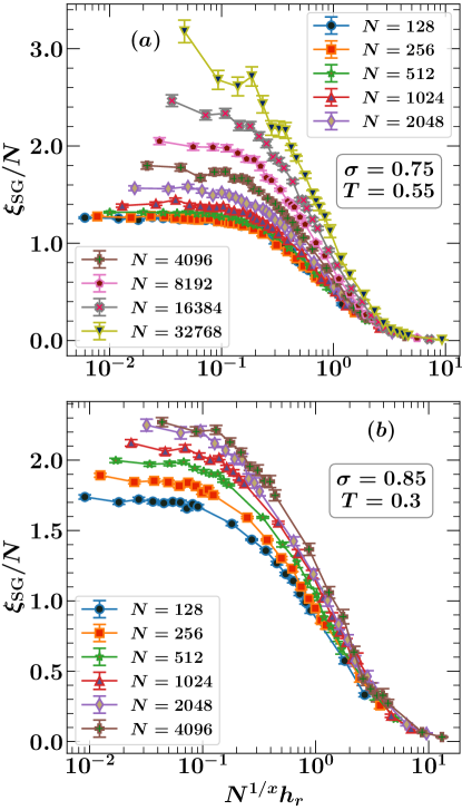
Figure 14: Finite size scaling plots of $\xi_{\text{SG}}$ as a function of magnetic field $h_{r}$, for (a) $\sigma=0.75$ at a temperature of $T=0.55$, and (b) $\sigma=0.85$ at a temperature of $T=0.3$. These figures show $\xi_{\text{SG}}/N$ plotted on a linear scale versus $N^{1/x}h_{r}$ in the region where $\xi_{\text{SG}}/N$ is of $O(1)$

.

The results from our work are broadly in accord with those for the corresponding Heisenberg spin glass model. For $\sigma=0.6$, which is in the mean-field regime, we find a phase transition in the absence of an external magnetic field, and in the presence of a magnetic field, which indicates the existence of an AT line. The location of the AT line is close to the mean-field predictions. For $\sigma=0.75$, which is in the non-mean-field regime, the conventional data collapse suggests the existence of an AT line, but the behavior of the intersections as a function of $N$ indicate that the data is not close to its large $N$ asymptotic form. The estimated location of the AT field based upon intersections that we get from our data at $\sigma=0.75$ is strikingly smaller than estimates based on the mean-field theory formulas. For $\sigma=0.85$, which is deep in the non-mean-field regime and corresponds to a space dimension of about $3$, our data are consistent with the absence of an AT line. In this case there is no crossing of the curves of $\chi_{\text{SG}}/N^{2-\eta}$ versus $T$ at various $N$ values. But confusingly intersections $h^{*}(N,2N)$, as a function of $h_{r}$, seem to exist, whereas intersections $T^{*}(N,2N)$ are absent at least for $\sigma=0.85$.

However, for $\sigma=0.75$ and for $\sigma=0.85$ we found that the droplet picture provided a much better description of our data from that obtained assuming the existence of an AT transition line. The Imry-Ma formula for the field dependence of $\xi_{\text{SG}}$ works well until $\xi_{\text{SG}}$ becomes comparable to the system size. A similar behavior was reported for the Ising spin glass at $\sigma=0.75$ in Ref. [49]. A finite-size scaling formulation was developed to treat the data at small fields when $\xi_{\text{SG}}$ is comparable to the system size $N$, and with it an excellent collapse of all our data on $\xi_{\text{SG}}$ and $\chi_{\text{SG}}$ was obtained. We showed that droplet scaling predicts the existence of the intersections $h^{*}(N,2N)$. Our data unfortunately does not extend to values of $N$ large enough to be in the asymptotic region where the $N$-dependence of $h^{*}(N,2N)$ is simple. Fortunately there exists a way of testing whether the intersections are due to an AT transition or are just those predicted by droplet scaling, which is to study the $N$ dependence of $R=\chi_{\text{SG}}/N^{2\sigma-1}$, calculated at $h^{*}(N,2N)$, and this test supports the droplet picture provided $N>1024$ at $\sigma=0.75$. Thus it is only for large systems that one can obtain good evidence for the droplet picture.

We now summarize our main results. The strongest evidence for droplet scaling is the success of the Imry-Ma formula for the field dependence of $\xi_{\text{SG}}$ for $\sigma=0.75$ and $\sigma=0.85$ (see inset Figs. 10(e) and 10(f)). If droplet scaling works, then no AT line is to be expected. When $\xi_{\text{SG}}\sim N$ there are visible sizeable corrections to the Imry-Ma formula which are related to TNT effects. However for $\sigma=0.85$ there is tentative evidence in Fig. 14(b) that if even larger systems could be studied then the TNT effects might be absent, and so there could exist a length scale $L^{*}$ above which TNT effects become unimportant (see Ref. [3]). If instead of droplet scaling one assumes that there is an AT phase transition then the usual finite size scaling plots used to determine $h_{\text{AT}}$ as in Fig. 5(c) for $\sigma=0.75$ are unsatisfactory: for example the values of $h_{\text{AT}}$ which would be derived from the crossings of $\xi_{\text{SG}}$ and $\chi_{\text{SG}}$ as $N$ becomes large look to be significantly different. In the equivalent data plot for $\sigma=0.60$ (see Fig.  3(c)) they are in good agreement. Furthermore the quantity $R$ of Eq. (35) should approach a constant as $N\to\infty$ if there is a genuine AT transition, but instead for the cases $\sigma=0.75$ (Fig. 12(b)) and $0.85$ (Fig. 12(c)), it is increasing with $N$ once $N$ becomes large enough.

The simulations of this paper provide numerical evidence that the AT line and hence RSB is absent in spin glasses below six dimensions. What is now needed is an explanation of why this might be the case. Better still would be a rigorous proof that the lower critical dimension for replica symmetry breaking is six. Our work indicates that showing that $\sigma=2/3$ is the precise value of the critical value of $\sigma$ will be challenging using simulations as finite size effects are large in its vicinity.

Appendix A The simulation method

We now give some technical aspects of how the simulations are run. In the simulations we start with a random initial configuration and allow it to evolve according to the prescription given in this section. To incorporate parallel tempering, we simultaneously simulate $N_{T}$ copies of the system over $N_{T}$ different temperatures ranging from $T_{\text{min}}\equiv T_{1}$ to $T_{\text{max}}\equiv T_{N_{T}}$. In order to facilitate the computation of the observables outlined in this section, it is convenient to simulate $4$ sets of $N_{T}$ copies (2 for $h_{r}=0$), which we label (1),(2),(3), and (4). We perform overrelaxation, heatbath and parallel tempering sweeps over all these copies keeping track of the labels appropriately. For every $10$ overrelaxation sweeps we perform $1$ heatbath and $1$ parallel tempering sweep, since the overrelaxation sweep involves a significantly lower computational cost, and is known to speed up equilibration. The parameters of the simulations are shown in Tables 3 and 4. Once the system reaches equilibrium, we perform the same number of sweeps in the measurement phase, so $N_{\text{sweep}}$ is the total number of sweeps over which the simulation is run, inclusive of both the equilibration and measurement phases. The last column in the table shows the amount of computer time expended to generate the data corresponding to the parameters in that row. In the measurement phase, we perform one measurement on the system for every $4$ sweeps. The following sections contain the details of our Monte Carlo simulation procedures. In order to equilibrate the system as quickly as possible, we perform three kinds of sweeps: overrelaxation or microcanonical sweeps, heatbath sweeps, and parallel tempering sweeps.

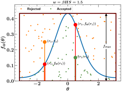
Figure 15: Graphical representation of the rejection method. We randomly pick a point $(r_{1},r_{2})$ within the rectangle from a uniform distribution. If the point lies under the $f_{\Theta}(\theta)$ curve given by Eq. (38), then the point is accepted, and $\theta$ is taken to be $r_{1}$. Otherwise, the point is rejected.

A.1 Overrelaxation sweep

We sweep sequentially through all the lattice sites and compute the local field $\mathbf{H}_{i}=\sum_{j}J_{ij}\mathbf{S}_{j}+\mathbf{h}_{i}$ at a particular lattice site. The new spin direction $\mathbf{S}^{\prime}_{i}$ at the $i^{\text{th}}$ lattice site is taken to be the mirror image of the vector $\mathbf{S}_{i}$ about $\mathbf{H}_{i}$, i.e.,

$$\mathbf{S}^{\prime}_{i}=-\mathbf{S}_{i}+2\frac{\mathbf{S}_{i}\cdot\mathbf{H}_{i}}{H_{i}^{2}}\mathbf{H}_{i}.$$ (37)

Since $\mathbf{S}^{\prime}_{i}\cdot\mathbf{H}_{i}=\mathbf{S}_{i}\cdot\mathbf{H}_{i}$, the energy of the system does not change due to these sweeps. Hence these sweeps are also called microcanonical sweeps. These sweeps help us in sampling out the microstates with the same energy. The process of equilibration speeds up when we include overrelaxation sweeps along with the other sweeps [33, 53].

A.2 Heatbath sweep

The overrelaxation sweeps generate states with the same energy and hence they cannot directly equilibrate the system. Therefore, we also perform a heatbath sweep for every $10$ microcanonical sweeps. Similar to the microcanonical case, we sweep sequentially through the lattice.

To equilibrate the system, the angle $\theta$ between $\mathbf{H_{i}}$ and $\mathbf{S^{{}^{\prime}}_{i}}$ should be sampled out from the Boltzmann distribution given by

$$f_{\Theta}(\theta)=\frac{\text{e}^{-\beta E_{i}}}{Z}=\frac{\text{e}^{\beta H_{i}S_{i}\cos\theta}}{Z}=\frac{\text{e}^{w\cos\theta}}{Z}\,,$$ (38)

where $w=\beta H_{i}S_{i}$ and

$$Z=\int\limits_{-\pi}^{\pi}\text{e}^{\beta H_{i}S_{i}\cos\theta}\,d\theta$$ (39)

is the normalizing constant. The simplest way to do this is to equate the cumulative density function (CDF) of $\theta$, $F_{\Theta}(\theta)$, to that of a uniform distribution:

$$F_{\Theta}(\theta)=\int\limits_{-\pi}^{\theta}f_{\Theta}(\theta^{\prime})\,d\theta^{\prime}=\Pi(r_{1})=r_{1},$$ (40)

where $r_{1}$ is a random variable sampled from a uniform distribution in the interval $(0,1)$. The value of $\theta$ can be obtained by simply inverting this function to get

$$\theta=F_{\Theta}^{-1}(r_{1}).$$ (41)

This method works well with the Heisenberg spins as $f_{\Theta}(\theta)$ is integrable, which gives an invertible CDF $F_{\Theta}(\theta)$ [18, 28]. Since the probabililty density function (PDF) $f_{\Theta}(\theta)$ for the XY spin glasses given by Eq. (38) is not exactly integrable, this method cannot be used.

To overcome this problem and to sample out $\theta$ from the Boltzmann distribution (Eq. (38)) in as few a number of sweeps as possible, we develop a heatbath sweep based on the rejection method [54] We generate two random numbers $r_{1}\in\text{uniform}(-\pi,\pi)$ and $r_{2}\in\text{uniform}(0,f_{\text{max}})$. If $r_{2}<f_{\theta}(r_{1})$, we accept the move, i.e., take $\theta=r_{1}$. Else, we reject the move and generate another pair of random numbers $(r_{1},r_{2})$. This process is repeated until we find an acceptable value of $r_{1}$. A graphical representation for this method is shown in Fig. 15. The new spin direction $\mathbf{S}^{\prime}_{i}$ in Cartesian co-ordinates is given by:

$$S^{\prime}_{x} =\cos(\theta+\theta_{H}),$$ (42a)

$$S^{\prime}_{y} =\sin(\theta+\theta_{H}),$$ (42b)

where $\theta_{H}$ is the angle made by the $\mathbf{H}_{i}$ vector with the $X$-axis. Since the generation of random numbers is involved, this sweep is computationally costlier than others. Hence we perform more microcanonical sweeps than heatbath sweeps.

Table 3: Parameters of the simulations. $N_{\text{samp}}$ is the number of disorder samples, $N_{\text{sweep}}$ is the number of over-relaxation Monte Carlo sweeps for a single disorder sample. The system is equilibrated over the first half of the sweeps, and measurements are done over the last half of the sweeps with a measurement performed every four over-relaxation sweeps. $T_{\text{min}}$ and $T_{\text{max}}$ are the lowest and highest temperatures simulated, and $N_{T}$ is the number of temperatures used for parallel tempering.

$\sigma$	$h_{r}$	$N$	$N_{\text{samp}}$	$N_{\text{sweep}}$	$T_{\text{min}}$	$T_{\text{max}}$	$N_{T}$	$t_{\text{tot}}$(hrs)
0.6	0	128	10000	512	0.6	1	18	0.49
0.6	0	256	8000	1024	0.6	1	22	2.23
0.6	0	512	6400	2048	0.6	1	22	6.46
0.6	0	1024	8000	4096	0.6	1	26	40.74
0.6	0	2048	3840	8192	0.6	1	24	105.41
0.6	0	4096	3200	16384	0.6	1	27	571.49
0.6	0	8192	3200	32768	0.6	1	30	3776.85
0.6	0	16384	2600	65536	0.64	0.98	32	18225.5
0.6	0.1	128	9600	2048	0.5	0.8	21	7.75
0.6	0.1	256	9600	2048	0.5	0.8	21	15.89
0.6	0.1	512	9600	8192	0.5	0.8	22	85.67
0.6	0.1	1024	8000	16384	0.5	0.8	22	414.47
0.6	0.1	2048	7200	32768	0.5	0.8	26	2029.23
0.6	0.1	4096	7200	65536	0.5	0.8	24	10014.8
0.6	0.1	8192	4380	131072	0.55	0.8	25	34810.6
0.6	0.1	16384	7128	262144	0.55	0.8	28	224425
0.75	0	128	12800	1024	0.35	0.85	21	1.6
0.75	0	256	12800	2048	0.35	0.85	24	7.21
0.75	0	512	8000	8192	0.35	0.85	24	35.22
0.75	0	1024	8000	16384	0.35	0.85	24	196.9
0.75	0	2048	6400	32768	0.35	0.85	25	774.55
0.75	0	4096	4880	65536	0.35	0.85	27	3405.2
0.75	0	8192	3000	131072	0.38	0.82	30	14290.9
0.75	0.05	128	19200	8192	0.28	0.6	21	45.27
0.75	0.05	256	16000	16384	0.28	0.6	20	133.35
0.75	0.05	512	13600	32768	0.28	0.6	20	464.77
0.75	0.05	1024	11000	65536	0.28	0.6	21	2075.57
0.75	0.05	2048	10920	262144	0.28	0.6	24	21314.3
0.75	0.05	4096	10800	524288	0.3	0.58	26	123093
0.75	0.05	8192	5320	1048576	0.32	0.54	32	364358
0.85	0	128	12800	8192	0.2	0.5	30	17.97
0.85	0	256	12800	16384	0.2	0.5	32	72.15
0.85	0	512	12800	65536	0.2	0.5	30	752.36
0.85	0	1024	12800	131072	0.2	0.5	30	3219.93
0.85	0	2048	8000	262144	0.2	0.5	30	9504.05
0.85	0	4096	6480	524288	0.24	0.48	30	40322.4
0.85	0.02	128	8000	65536	0.1	0.4	30	194.33
0.85	0.02	256	4000	131072	0.1	0.4	32	470.39
0.85	0.02	512	4400	524288	0.1	0.4	34	4780.6
0.85	0.02	1024	3000	2097152	0.1	0.4	35	30356.9
0.85	0.02	2048	1800	4194304	0.16	0.4	36	84056
0.85	0.05	128	2000	65536	0.1	0.4	30	67.07
0.85	0.05	256	4000	131072	0.1	0.4	32	604.8
0.85	0.05	512	3500	524288	0.1	0.4	36	4958.17
0.85	0.05	1024	3120	2097152	0.1	0.4	36	28028.1
0.85	0.05	2048	3240	4194304	0.16	0.4	36	151503

Table 4: Parameters of the simulations done at fixed temperature $T$ and varying field $h_{r}$. $N(h_{r})$ is the number of values of field taken in the range $h_{r}$(min,max). The equilibration times are different for different values of the field $h_{r}$, which lie in the range $N_{\text{sweep}}$(min,max). The number of disorder samples for different fields lie in the range $N_{\text{samp}}$(min,max). $t_{\text{tot}}$ is the total CPU time consumed in hours to generate data for a particular system size.

$\sigma$	$T$	$N$	$h_{r}$(min,max)	$N(h_{r})$	$N_{\text{sweep}}$(min,max)	$N_{\text{samp}}$(min,max)	$t_{\text{tot}}$(hrs)
0.6	0.6	128	$(0.010,9.000)$	32	$(2048,2048)$	$(2000,64000)$	11.44
0.6	0.6	256	$(0.010,9.000)$	32	$(4096,4096)$	$(2000,48000)$	55.5
0.6	0.6	512	$(0.010,9.000)$	32	$(8192,16384)$	$(2000,80000)$	163.91
0.6	0.6	1024	$(0.010,9.000)$	32	$(4096,65536)$	$(2000,80000)$	2375
0.6	0.6	2048	$(0.010,9.000)$	32	$(16384,131072)$	$(1200,60000)$	10259.8
0.6	0.6	4096	$(0.010,9.000)$	32	$(65536,2097152)$	$(960,28600)$	92052.1
0.6	0.6	8192	$(0.010,9.000)$	32	$(65536,4194304)$	$(400,19428)$	310948
0.6	0.6	16384	$(0.010,9.000)$	32	$(131072,4194304)$	$(488,10689)$	1021481
0.7	0.6	128	$(0.010,9.000)$	31	$(1024,1024)$	$(4000,4000)$	1.86
0.7	0.6	256	$(0.010,9.000)$	31	$(2048,2048)$	$(1000,8000)$	8.53
0.7	0.6	512	$(0.010,9.000)$	31	$(4096,4096)$	$(1000,8000)$	39.46
0.7	0.6	1024	$(0.010,9.000)$	31	$(8192,8192)$	$(1500,8000)$	288.41
0.7	0.6	2048	$(0.010,9.000)$	31	$(16384,16384)$	$(500,8000)$	559.99
0.7	0.6	4096	$(0.010,9.000)$	31	$(32768,32768)$	$(400,8000)$	3020.62
0.7	0.6	8192	$(0.010,9.000)$	31	$(16384,131072)$	$(2000,6800)$	17500.2
0.7	0.6	16384	$(0.010,9.000)$	31	$(32768,262144)$	$(640,6400)$	77734.3
0.75	0.55	128	$(0.001,9.000)$	42	$(512,1024)$	$(2000,40000)$	6.59
0.75	0.55	256	$(0.001,9.000)$	42	$(1024,2048)$	$(2000,40000)$	56.67
0.75	0.55	512	$(0.001,9.000)$	42	$(4096,4096)$	$(1000,24000)$	165.51
0.75	0.55	1024	$(0.001,9.000)$	43	$(8192,8192)$	$(1000,12000)$	255.75
0.75	0.55	2048	$(0.001,9.000)$	43	$(16384,16384)$	$(1000,12000)$	1000.52
0.75	0.55	4096	$(0.001,9.000)$	43	$(32768,32768)$	$(800,12000)$	5269.11
0.75	0.55	8192	$(0.001,9.000)$	42	$(65536,65536)$	$(800,8000)$	21410.3
0.75	0.55	16384	$(0.001,9.000)$	42	$(131072,131072)$	$(760,6280)$	62062
0.75	0.55	32768	$(0.001,9.000)$	42	$(131072,262144)$	$(512,4995)$	146627
0.85	0.3	128	$(0.001,9.000)$	36	$(32768,131072)$	$(2000,30000)$	264.97
0.85	0.3	256	$(0.001,9.000)$	36	$(65536,262144)$	$(1000,25000)$	1052.21
0.85	0.3	512	$(0.001,9.000)$	36	$(131072,524288)$	$(1000,34800)$	6161.52
0.85	0.3	1024	$(0.001,9.000)$	36	$(262144,1048576)$	$(1000,20000)$	17668
0.85	0.3	2048	$(0.001,9.000)$	36	$(524288,8388608)$	$(320,3372)$	68933.6
0.85	0.3	4096	$(0.001,9.000)$	36	$(262144,16777216)$	$(312,5760)$	439004

A.3 Parallel tempering sweep

Spin glasses have a complex free energy landscape due to which, at low temperatures, they tend to get stuck inside metastable valleys, and true equilibration consumes a lot of time. At high temperatures, the system can easily escape the valley due to thermal fluctuations, and so equilibration is quick. To equilibrate the system in as small a number of moves as possible, we perform one parallel tempering sweep for every $10$ overrelaxation sweeps [28, 33]. To benefit from the parallel tempering algorithm [55, 56], we simultaneously run the simulation for $N_{T}$ copies of the system at $N_{T}$ different temperatures $T_{1}<T_{2}<T_{3}<\cdots<T_{N_{T}}$. The minimum temperature $T_{1}$ is the low temperature at which we are interested in studying the behavior of the system, and the maximum temperature $T_{N_{T}}$ is high enough that the system equilibrates very fast. We perform overrelaxation and heatbath sweeps separately on each of the $N_{T}$ copies of the system. In the parallel tempering sweep, we compare the energies of two spin configurations at adjacent temperatures, $T_{i}$ and $T_{i+1}$, starting from the smallest temperature $T_{1}$. We swap these two spin configurations such that the detailed balance condition is satisfied. The Metropolis probability for such a swap is

$$P(T\text{ swap}) =\min\{1,\exp(\Delta\beta\Delta E)\}$$ (43)

$$=\begin{cases}\exp(\Delta\beta\Delta E),&(\text{if }\Delta\beta\Delta E<0),\\ 1,&(\text{otherwise}),\end{cases}$$ (44)

where $\Delta\beta=1/T_{i}-1/T_{i+1}$ and $\Delta E=E_{i}(T_{i})-E_{i+1}(T_{i+1})$. In this way, a given set of spins performs a random walk in temperature space.

A.4 Checks for equilibration

In order to check whether the system has reached equilibrium, we have used a convenient test [57] which is possible because of the Gaussian nature of the interactions and the onsite external magnetic field. The relation

$$U=\frac{zJ^{2}}{2T}\left(q_{l}-q_{s}\right)+\frac{h_{r}^{2}}{T}\left(q-\left|\textbf{S}\right|^{2}\right),$$ (45)

is valid in equilibrium. Here

$$U =\frac{1}{N}\left[\langle\mathcal{H}\rangle\right]_{\text{av}}$$

$$=-\frac{1}{N}\left[\sum\limits_{\langle i,j\rangle}\epsilon_{ij}J_{ij}\left\langle\textbf{S}_{i}\cdot\textbf{S}_{j}\right\rangle+\sum\limits_{i,\mu}h_{i}^{\mu}\left\langle S_{i}^{\mu}\right\rangle\right]_{\text{av}}$$ (46)

is the average energy per spin, $q=\frac{1}{N}\sum\limits_{i}\left[\left\langle\textbf{S}_{i}\right\rangle\cdot\left\langle\textbf{S}_{i}\right\rangle\right]_{\text{av}}$ is the Edwards-Anderson order parameter, $q_{l}=\frac{1}{N_{b}}\sum_{\langle i,j\rangle}\left[\epsilon_{ij}\left\langle\textbf{S}_{i}\cdot\textbf{S}_{j}\right\rangle^{2}\right]_{\text{av}}$ is the “link overlap”, and $q_{s}=\frac{1}{N_{b}}\sum_{\langle i,j\rangle}\left[\epsilon_{ij}\left\langle\left(\textbf{S}_{i}\cdot\textbf{S}_{j}\right)^{2}\right\rangle\right]_{\text{av}}$ is the “spin overlap”, where $N_{b}=Nz/2$, and $\epsilon_{ij}=1$ if the $i^{\text{th}}$ and $j^{\text{th}}$ spins are interacting and is zero otherwise. The $[\cdots]_{\text{av}}$ in Eq. (A.4) is analytically evaluated by performing integration over $J_{ij}$ and $h_{i}^{\mu}$ [58] since they have Gaussian distributions. On evaluating this integral using integration by parts, we get Eq. (45). As the system reaches equilibrium, the two sides of Eq. (45) approach their common equilibrium value from opposite directions.

In simulations, we evaluate both sides of Eq. (45) for different number of Monte-Carlo sweeps (MCSs), which increase in an exponential manner, each value being twice the previous one. The averaging is done over the last half of the sweeps. We initially start with a random spin configuration, so the LHS of Eq. (45) is small and the RHS is very large. As the system gets closer to equilibrium, these two values come closer to each other from opposite directions. When we notice that the averaged quantities satisfy Eq. (45) within error bars, consistently for at least the last two points, we declare that our system has reached equilibrium. Once the system reaches equilibrium, we perform the same number of sweeps in the measurement phase, where we evaluate different quantities (given below) used to study the possible phase transitions of the system.

References

- Mézard et al. [1986] M. Mézard, G. Parisi, and M. A. Virasoro, Spin glass theory and beyond: An Introduction to the Replica Method and Its Applications, Vol. 9 (World Scientific Publishing Company, 1986).
- de Almeida and Thouless [1978] J. R. L. de Almeida and D. J. Thouless, Stability of the Sherrington-Kirkpatrick solution of a spin glass model, Journal of Physics A: Mathematical and General 11, 983 (1978).
- Moore [2021] M. A. Moore, Droplet-scaling versus replica symmetry breaking debate in spin glasses revisited, Phys. Rev. E 103, 062111 (2021).
- Martin-Mayor et al. [2022] V. Martin-Mayor, J. J. Ruiz-Lorenzo, B. Seoane, and A. P. Young, Numerical simulations and replica symmetry breaking (2022), arXiv:2205.14089 [cond-mat.dis-nn] .
- Sharma and Young [2010] A. Sharma and A. P. Young, de Almeida–Thouless line in vector spin glasses, Phys. Rev. E 81, 061115 (2010).
- Bray and Roberts [1980] A. J. Bray and S. A. Roberts, Renormalisation-group approach to the spin glass transition in finite magnetic fields, Journal of Physics C: Solid State Physics 13, 5405 (1980).
- Moore and Bray [2011] M. A. Moore and A. J. Bray, Disappearance of the de Almeida-Thouless line in six dimensions, Phys. Rev. B 83, 224408 (2011).
- Kotliar et al. [1983] G. Kotliar, P. W. Anderson, and D. L. Stein, One-dimensional spin-glass model with long-range random interactions, Phys. Rev. B 27, 602 (1983).
- Dyson [1969] F. J. Dyson, Non-existence of spontaneous magnetization in a one-dimensional Ising ferromagnet, Communications in Mathematical Physics 12, 212 (1969).
- Dyson [1971] F. J. Dyson, An Ising ferromagnet with discontinuous long-range order, Communications in Mathematical Physics 21, 269 (1971).
- Leuzzi et al. [2008] L. Leuzzi, G. Parisi, F. Ricci-Tersenghi, and J. J. Ruiz-Lorenzo, Dilute One-Dimensional Spin Glasses with Power Law Decaying Interactions, Phys. Rev. Lett. 101, 107203 (2008).
- Leuzzi et al. [2009] L. Leuzzi, G. Parisi, F. Ricci-Tersenghi, and J. J. Ruiz-Lorenzo, Ising Spin-Glass Transition in a Magnetic Field Outside the Limit of Validity of Mean-Field Theory, Phys. Rev. Lett. 103, 267201 (2009).
- Young and Katzgraber [2004] A. P. Young and H. G. Katzgraber, Absence of an Almeida-Thouless Line in Three-Dimensional Spin Glasses, Phys. Rev. Lett. 93, 207203 (2004).
- Katzgraber and Young [2005] H. G. Katzgraber and A. P. Young, Probing the Almeida-Thouless line away from the mean-field model, Phys. Rev. B 72, 184416 (2005).
- Katzgraber et al. [2009] H. G. Katzgraber, D. Larson, and A. P. Young, Study of the de Almeida–Thouless Line Using Power-Law Diluted One-Dimensional Ising Spin Glasses, Phys. Rev. Lett. 102, 177205 (2009).
- Katzgraber and Young [2003] H. G. Katzgraber and A. P. Young, Monte Carlo studies of the one-dimensional Ising spin glass with power-law interactions, Phys. Rev. B 67, 134410 (2003).
- Sharma and Young [2011a] A. Sharma and A. P. Young, Phase transitions in the one-dimensional long-range diluted Heisenberg spin glass, Phys. Rev. B 83, 214405 (2011a).
- Sharma and Young [2011b] A. Sharma and A. P. Young, de Almeida–Thouless line studied using one-dimensional power-law diluted Heisenberg spin glasses, Phys. Rev. B 84, 014428 (2011b).
- Sharma et al. [2016] A. Sharma, J. Yeo, and M. A. Moore, Metastable minima of the Heisenberg spin glass in a random magnetic field, Phys. Rev. E 94, 052143 (2016).
- Beyer et al. [2012] F. Beyer, M. Weigel, and M. A. Moore, One-dimensional infinite-component vector spin glass with long-range interactions, Phys. Rev. B 86, 014431 (2012).
- Moore [2012] M. A. Moore, expansion in spin glasses and the de Almeida-Thouless line, Phys. Rev. E 86, 031114 (2012).
- Sharma et al. [2014] A. Sharma, A. Andreanov, and M. Müller, Avalanches and hysteresis in frustrated superconductors and spin glasses, Phys. Rev. E 90, 042103 (2014).
- Franz et al. [2022] S. Franz, F. Nicoletti, G. Parisi, and F. Ricci-Tersenghi, Delocalization transition in low energy excitation modes of vector spin glasses, SciPost Phys. 12, 16 (2022).
- Lupo and Ricci-Tersenghi [2018] C. Lupo and F. Ricci-Tersenghi, Comparison of Gabay–Toulouse and de Almeida–Thouless instabilities for the spin-glass XY model in a field on sparse random graphs, Phys. Rev. B 97, 014414 (2018).
- Lupo et al. [2019] C. Lupo, G. Parisi, and F. Ricci-Tersenghi, The random field XY model on sparse random graphs shows replica symmetry breaking and marginally stable ferromagnetism, Journal of Physics A: Mathematical and Theoretical 52, 284001 (2019).
- Baity-Jesi et al. [2015] M. Baity-Jesi, V. Martín-Mayor, G. Parisi, and S. Perez-Gaviro, Soft Modes, Localization, and Two-Level Systems in Spin Glasses, Phys. Rev. Lett. 115, 267205 (2015).
- Fernandez et al. [2009] L. A. Fernandez, V. Martin-Mayor, S. Perez-Gaviro, A. Tarancon, and A. P. Young, Phase transition in the three dimensional Heisenberg spin glass: Finite-size scaling analysis, Phys. Rev. B 80, 024422 (2009).
- Lee and Young [2007] L. W. Lee and A. P. Young, Large-scale Monte Carlo simulations of the isotropic three-dimensional Heisenberg spin glass, Phys. Rev. B 76, 024405 (2007).
- Campos et al. [2006] I. Campos, M. Cotallo-Aban, V. Martin-Mayor, S. Perez-Gaviro, and A. Tarancon, Spin-Glass Transition of the Three-Dimensional Heisenberg Spin Glass, Phys. Rev. Lett. 97, 217204 (2006).
- Olive et al. [1986] J. A. Olive, A. P. Young, and D. Sherrington, Computer simulation of the three-dimensional short-range Heisenberg spin glass, Phys. Rev. B 34, 6341 (1986).
- Hukushima and Kawamura [2000] K. Hukushima and H. Kawamura, Chiral-glass transition and replica symmetry breaking of a three-dimensional Heisenberg spin glass, Phys. Rev. E 61, R1008 (2000).
- Viet and Kawamura [2009] D. X. Viet and H. Kawamura, Numerical Evidence of Spin-Chirality Decoupling in the Three-Dimensional Heisenberg Spin Glass Model, Phys. Rev. Lett. 102, 027202 (2009).
- Pixley and Young [2008] J. H. Pixley and A. P. Young, Large-scale Monte Carlo simulations of the three-dimensional spin glass, Phys. Rev. B 78, 014419 (2008).
- Berganza and Leuzzi [2013] M. I. n. Berganza and L. Leuzzi, Critical behavior of the model in complex topologies, Phys. Rev. B 88, 144104 (2013).
- Baity-Jesi et al. [2014] M. Baity-Jesi, R. A. Baños, A. Cruz, L. A. Fernandez, J. M. Gil-Narvion, A. Gordillo-Guerrero, D. Iñiguez, A. Maiorano, F. Mantovani, E. Marinari, V. Martin-Mayor, J. Monforte-Garcia, A. M. Sudupe, D. Navarro, G. Parisi, S. Perez-Gaviro, M. Pivanti, F. Ricci-Tersenghi, J. J. Ruiz-Lorenzo, S. F. Schifano, B. Seoane, A. Tarancon, R. Tripiccione, and D. Yllanes, The three-dimensional Ising spin glass in an external magnetic field: the role of the silent majority, Journal of Statistical Mechanics: Theory and Experiment 2014, P05014 (2014).
- Krzakala and Martin [2000] F. Krzakala and O. C. Martin, Spin and Link Overlaps in Three-Dimensional Spin Glasses, Phys. Rev. Lett. 85, 3013 (2000).
- Palassini and Young [2000] M. Palassini and A. P. Young, Nature of the Spin Glass State, Phys. Rev. Lett. 85, 3017 (2000).
- Sherrington and Kirkpatrick [1975] D. Sherrington and S. Kirkpatrick, Solvable Model of a Spin-Glass, Phys. Rev. Lett. 35, 1792 (1975).
- Larson et al. [2010] D. Larson, H. G. Katzgraber, M. A. Moore, and A. P. Young, Numerical studies of a one-dimensional three-spin spin-glass model with long-range interactions, Phys. Rev. B 81, 064415 (2010).
- de Almeida et al. [1978] J. R. L. de Almeida, R. C. Jones, J. M. Kosterlitz, and D. J. Thouless, The infinite-ranged spin glass with m-component spins, Journal of Physics C: Solid State Physics 11, L871 (1978).
- Baños et al. [2012] R. A. Baños, L. A. Fernandez, V. Martin-Mayor, and A. P. Young, Correspondence between long-range and short-range spin glasses, Phys. Rev. B 86, 134416 (2012).
- Binder [1981] K. Binder, Finite size scaling analysis of Ising model block distribution functions, Zeitschrift für Physik B Condensed Matter 43, 119 (1981).
- Ballesteros et al. [1996] H. Ballesteros, L. Fernández, V. Martín-Mayor, and A. Muñoz Sudupe, Finite size effects on measures of critical exponents in d = 3 O(N) models, Physics Letters B 387, 125 (1996).
- Hasenbusch et al. [2008] M. Hasenbusch, A. Pelissetto, and E. Vicari, Critical behavior of three-dimensional Ising spin glass models, Phys. Rev. B 78, 214205 (2008).
- McMillan [1984] W. L. McMillan, Scaling theory of Ising spin glasses, Journal of Physics C: Solid State Physics 17, 3179 (1984).
- Bray and Moore [1986] A. J. Bray and M. A. Moore, Scaling Theory of the ordered phase of spin glasses, in Heidelberg Colloquium on Glassy Dynamics and Optimization, edited by L. Van Hemmen and I. Morgenstern (Springer, New York, 1986) p. 121.
- Fisher and Huse [1988] D. S. Fisher and D. A. Huse, Equilibrium behavior of the spin-glass ordered phase, Phys. Rev. B 38, 386 (1988).
- Imry and Ma [1975] Y. Imry and S.-k. Ma, Random-Field Instability of the Ordered State of Continuous Symmetry, Phys. Rev. Lett. 35, 1399 (1975).
- Aspelmeier et al. [2016a] T. Aspelmeier, H. G. Katzgraber, D. Larson, M. A. Moore, M. Wittmann, and J. Yeo, Finite-size critical scaling in Ising spin glasses in the mean-field regime, Phys. Rev. E 93, 032123 (2016a).
- Aspelmeier et al. [2016b] T. Aspelmeier, W. Wang, M. A. Moore, and H. G. Katzgraber, Interface free-energy exponent in the one-dimensional Ising spin glass with long-range interactions in both the droplet and broken replica symmetry regions, Phys. Rev. E 94, 022116 (2016b).
- Newman and Stein [2003] C. M. Newman and D. L. Stein, Finite-Dimensional Spin Glasses: States, Excitations, and Interfaces, Ann. Henri Poincaré 4, 497 (2003).
- Newman et al. [2022] C. M. Newman, N. Read, and D. L. Stein, Metastates and replica symmetry breaking (2022), arXiv:2204.10345 [cond-mat.dis-nn] .
- Alonso et al. [1996] J. L. Alonso, A. Tarancón, H. G. Ballesteros, L. A. Fernández, V. Martín-Mayor, and A. Muñoz Sudupe, Monte Carlo study of O(3) antiferromagnetic models in three dimensions, Phys. Rev. B 53, 2537 (1996).
- Larson and Odoni [1981] R. C. Larson and A. R. Odoni, Urban operations research (Prentice-Hall, Englewood Cliffs, N.J, 1981).
- Hukushima and Nemoto [1996] K. Hukushima and K. Nemoto, Exchange monte carlo method and application to spin glass simulations, Journal of the Physical Society of Japan 65, 1604 (1996).
- Machta [2009] J. Machta, Strengths and weaknesses of parallel tempering, Phys. Rev. E 80, 056706 (2009).
- Katzgraber et al. [2001] H. G. Katzgraber, M. Palassini, and A. P. Young, Monte Carlo simulations of spin glasses at low temperatures, Phys. Rev. B 63, 184422 (2001).
- Bray and Moore [1980] A. J. Bray and M. A. Moore, Some observations on the mean-field theory of spin glasses, Journal of Physics C: Solid State Physics 13, 419 (1980).