Deciphering Core, Valence and Double-Core-Polarization Contributions to Parity Violating Amplitudes in ¹³³Cs using Different Methods

Abstract

As a prerequisite of probing physics beyond the Standard Model (BSM) of particle physics, it is imperative to perform calculation of parity violating electric dipole ($E1_{PV}$) amplitudes within 0.5% accuracy in atomic systems. Latest high precision calculations of $E1_{PV}$ of the $6s~{}^{2}S\rightarrow 7s~{}^{2}S$ transition in ¹³³Cs by three different groups claim achieving its accuracy below 0.5%, but such claims contradict on the view that their final values differ by 1%. One of the major issues in these calculations is the opposite signs among the core correlation contribution from different works leading to 200% difference in its value. In a review [Rev. Mod. Phys. 90, 025008 (2018)], a Letter [Phys. Rev. D 103, L111303 (2021)] and a Comment [Phys. Rev. D 105, 018301 (2022)], reliability of all these calculations are strongly contended. We unearthed here the underlying reason for getting sign discrepancies in various works by investigating how different electron correlation effects are encapsulated through the undertaken methods in the above works to determine $E1_{PV}$. Detailed discussions presented in this work would help in guiding theoretical studies to improve accuracy of $E1_{PV}$ in atomic systems to probe BSM physics.

I Introduction

Atomic parity violation (APV) has implications for exploring physics beyond the Standard Model (SM) of particle physics [1, 2, 3]. The neutral current weak interactions due to exchange of the $Z_{0}$ bosons between electrons and nucleus in atomic systems lead to APV [4]. APV studies can offer a fundamental quantity known as nuclear weak charge $Q_{W}$, from which model independent values of electron-up and electron-down quarks coupling coefficients can be inferred [4, 5]. Hence, any deviations of these values from the SM can be used to probe new physics or to complement some of the findings of the Large Hadron Collider facility when it is upgraded at the higher TeV energy scale. The nuclear spin-independent (NSI) component of APV has been measured to an accuracy of 0.35% in the $6s~{}^{2}S_{1/2}-7s~{}^{2}S_{1/2}$ transition in ¹³³Cs [6]. Advanced experimental techniques have been proposed recently to improve accuracy of the above measurement, as well as carrying out similar measurement in the $6s~{}^{2}S_{1/2}-5d~{}^{2}D_{3/2}$ transition of ¹³³Cs [7, 8]. In order to extract $Q_{W}$ value from these measurements, it is imperative to perform calculation of the parity violating electric dipole ($E1_{PV}$) amplitudes of the corresponding transitions very precisely (arguably less than 0.5%).

There have been a long history of performing calculations of the $E1_{PV}$ amplitude for the $6s~{}^{2}S_{1/2}-7s~{}^{2}S_{1/2}$ transition in ¹³³Cs by employing different state-of-the-art relativistic atomic many-body theories at different levels of approximation. Among the early calculations, Dzuba et al had employed the time-dependent Hartree-Fock (TDHF) method [9, 10], while Mårtensson had applied the combined coupled-perturbed Dirac-Hartree-Fock (CPDF) method and random-phase approximation (RPA), together referred as CPDF-RPA method [11], to investigate the roles of core-polarization effects to $E1_{PV}$. Both these methods are technically equivalent, but Mårtensson had also provided results at the intermediate levels using approximations at the Dirac-Hartree-Fock (DHF), CPDF and RPA methods as well as listing contributions from double-core-polarization (DCP) effects explicitly. Later, Blundell et al had employed a linearized version relativistic coupled-cluster method in the singles and doubles excitation approximation (SD method) to estimate the $E1_{PV}$ amplitude of the above transition [12]. However, they had adopted a sum-over-states approach in which matrix elements of the electric dipole (E1) operator and APV interaction Hamiltonian were evaluated for the transitions involving $np~{}^{2}P_{1/2}$ intermediate states (called as “Main” contribution) with the principal quantum number $n=6-9$. This method also utilized the calculated E1 matrix elements and magnetic dipole hyperfine structure constants to estimate the uncertainty of $E1_{PV}$. Uncertainties from the energies were removed by considering the experimental energies, while contributions from core orbitals (referred as “Core” contribution henceforth) and higher $np~{}^{2}P_{1/2}$ intermediate states (hereafter called as “Tail” contribution) were estimated using lower-order methods. Following this work, Dzuba et al improved their calculation of TDHF method by incorporating correlation contributions through the Brückner orbitals (BO) and referred the approach as RPA$+$BO method [13]. Higher-order contributions from the Breit, lower-order QED and neutron skin effects were added subsequently through different works to claim for more precise $E1_{PV}$ value for extracting the BSM physics [14, 15, 16, 17, 18, 19, 20]. It is worth mentioning here that all these higher-order effects were estimated through different types of many-body methods and without accounting correlations among themselves. Soon after these theoretical results, relativistic coupled-cluster (RCC) theory with singles and doubles approximation (RCCSD method) was employed to treat both the electromagnetic and weak interactions on an equal footing [21, 22, 23]. Moreover, it also treated correlations among the Main, Core and Tail contributions to $E1_{PV}$ but its accuracy was an concern due to its ab initio nature and use of a relatively smaller basis size in the available computational resources at that time.

A decade ago, Porsev et al made further improvement in the sum-over-states result of Blundell et al by considering contributions from the non-linear terms from RCCSD method to their SD method as well as adding valence triple excitations (CCSDvT method) [24]. Their claimed accuracy to the $E1_{PV}$ amplitude of the $6s~{}^{2}S_{1/2}-7s~{}^{2}S_{1/2}$ transition in ¹³³Cs was about 0.27%. However, the Core and Tail contributions were still estimated using a blend of many-body methods without explicitly stating which physical effects were taken into account for their evaluations. We refer these two contributions together as X-factor in this work. In an attempt to improve the calculated $E1_{PV}$ value further, Dzuba et al estimated the X-factor contributions using their TDHF approach but omitting the DCP contributions [25] in the similar line to their earlier works [9, 10]. This calculation showed an opposite sign of Core contribution than that was reported by Porsev et al. In 2013, Roberts reported the DCP contribution separately [26] and the result was slightly different than the value of Mårtensson [11]. The opposite sign of the Core contribution of Dzuba et al with Porcev et al was criticized in two papers [27, 28], which prompted for carrying out further investigation on different correlation contributions to $E1_{PV}$ from the first-principle approach. In 2021, Sahoo et al improved their calculation of the above $E1_{PV}$ amplitude by implementing the singles, doubles and triples approximation to both the unperturbed and perturbed wave functions (RCCSDT method) and using a much bigger set of basis functions [29]. They also used the same $V^{N-1}$ potential as in the previous cases and presented the Core and Valence (Main and Tail together) contributions explicitly. As per the convention adopted in this approach, the Core contribution agreed with the earlier RCCSD result [21, 22, 23], and was close to the reported value of Blundell et al [12] and Porsev et al [24]. In a recent Comment, Roberts and Ginges have argued in favour of opposite sign of Core contribution than other findings by giving intermediate results of their RPA$+$BO method [30]. In another work, Tan el al estimated combined Core and Tail contributions to the $E1_{PV}$ amplitude of the above transition using mixed-parity orbitals through RPA [31] and support the value reported in Ref. [24]. It is, therefore, abundantly clear that it is necessary to find out the issue of sign problem with the Core contribution to the above $E1_{PV}$ amplitude. More importantly, the basis of dividing net $E1_{PV}$ result into Core, Main, Tail, DCP, etc. contributions in an approach should be properly defined and missing physical effects in a method compared to others need to be well understood when a mixture of methods are used to estimate these contributions piece-wise. Any misinterpretation or misrepresentation of these contributions can have repercussion effect when they are used to infer beyond the SM (BSM) physics.

The present work is devoted to addressing the aforementioned sign issue with the Core contribution among various works, bringing to notice the shortcomings of the sum-over-states approach, and explaining the reason for the coincidental agreement between the core contributions of Porsev et al. [24] and Sahoo et al. [29]. We start with various procedures that can be adopted through a general many-body method to evaluate $E1_{PV}$ amplitudes in atomic systems and demonstrate how the definition of Core contribution can vary from one procedure to another. With the help of lower-order many-body methods, we find out the missing contributions in a typical sum-over-states approach to estimate $E1_{PV}$. We then analyze results from different methods to learn about how and to what extent these missing effects are incorporated in the previous calculations. We also make a similar analysis for the $E1_{PV}$ amplitude of the $6s~{}^{2}S_{1/2}-5d~{}^{2}D_{3/2}$ transition in ¹³³Cs and compare it with the result of the $6s~{}^{2}S_{1/2}-7s~{}^{2}S_{1/2}$ transition. There are two important reasons for quoting result of the $S-D_{3/2}$ transition of Cs here. First, our analysis would be helpful to estimate its $E1_{PV}$ amplitude more precisely which is required for the ongoing experiments [7, 8]. Second, we intend to address a comment [30, 32] on why sign for Core contribution to the $S-D_{3/2}$ transitions from different methods agree in contrast to the $S-S$ transitions.

II Theory

The short range effective Lagrangian corresponding to the vector- -axial-vector neutral weak current interaction of an electron with up- and down-quarks in an atomic system can be given by [33, 34, 35, 4]

$${\cal L}_{\rm eq} = \frac{G_{F}}{\sqrt{2}}\bar{\psi}_{e}\gamma^{\mu}\gamma^{5}\psi_{e}\sum_{u,d}\left[C_{1u}\bar{\psi}_{u}\gamma_{\mu}\psi_{u}+C_{1d}\bar{\psi}_{d}\gamma_{\mu}\psi_{d}\right]$$ (1)

$$= \frac{G_{F}}{\sqrt{2}}\bar{\psi}_{e}\gamma^{\mu}\gamma^{5}\psi_{e}\sum_{n}C_{1n}\bar{\psi}_{n}\gamma_{\mu}\psi_{n},$$

where $G_{F}=1.16632\times 10^{-5}$ GeV^-2 is the Fermi constant, sums $u$, $d$ and $n$ stand for up-quark, down-quark and nucleons respectively, and $C_{1i}$ with $i=u$, $d$ and $n$ represent coupling coefficients of the interaction of an electron with up-quark, down-quark and nucleons (protons (Pn) and neutrons (Nn)) respectively. Adding them coherently and taking the non-relativistic approximation for nucleons, the temporal component can give the nuclear-spin-independent APV interaction Hamiltonian as

$$H_{\rm PV}^{\rm NSI} = -\frac{G_{F}}{2\sqrt{2}}Q_{W}\gamma^{5}\rho(r),$$ (2)

where $\rho(r)$ is the averaged nuclear density and $Q_{W}=2[ZC_{1Pn}+(A-Z)C_{1Nn}]$ is known as the nuclear weak charge with $Z$ and $A$ representing for atomic and mass numbers respectively. It is obvious that $Q_{W}$ is a model dependent quantity. Thus, the difference of its actual value from the SM can provide signatures of physics supporting other models. In the SM, $C_{1u}=\frac{1}{2}\left[1-\frac{8}{3}\sin^{2}\theta_{W}^{\rm SM}\right]$ and $C_{1d}=-\frac{1}{2}\left[1-\frac{4}{3}\sin^{2}\theta_{W}^{\rm SM}\right]$ [33, 34, 35, 4]. This follows $C_{1Nn}=2C_{1d}+C_{1u}=-1/2$ and $C_{1Pn}=2C_{1u}+C_{1d}=(1-4\sin^{2}\theta_{W}^{\rm SM})/2\approx 0.04$, which are accurate up to 1%. Hence, it is necessary to evaluate model independent $Q_{W}$ in any atomic system within this accuracy in order to infer physics beyond the SM.

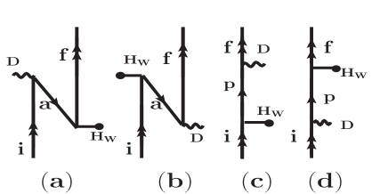
Figure 1: Goldstone diagrams representing Core (a and b) and Valence (c and d) contributions to $E1_{PV}$ in the $V^{N-1}$ DHF potential of an one valence atomic system. Here, double arrows represent initial ($i$) and final ($f$) valence orbitals, single arrows going down ($a$) means occupied orbitals and single arrows going up ($p$) means virtual orbitals. The operators $D$ and $H_{W}$ are shown in curly line and a line with bullet point respectively.

III Evaluation procedures of $E1_{PV}$

In the presence of APV, the net atomic Hamiltonian is given by

$$H_{at} = H+H_{\rm PV}^{\rm NSI}$$ (3)

$$= H+G_{F}H_{W},$$

where $H$ contains contributions from electromagnetic interactions and $H_{W}$ is defined in order to treat $G_{F}$ as a small parameter to include contributions from $H_{\rm PV}^{\rm NSI}$ perturbatively through a many-body method. Using the wave functions of $H_{at}$, we determine $E1_{PV}$ of a transition between states $|\Psi_{i}\rangle$ and $|\Psi_{f}\rangle$ as

$$E1_{PV}=\frac{\langle\Psi_{f}|D|\Psi_{i}\rangle}{\sqrt{\langle\Psi_{f}|\Psi_{f}\rangle\langle\Psi_{i}|\Psi_{i}\rangle}},$$ (4)

where $D$ is the E1 operator. In the earlier calculations of $E1_{PV}$ amplitude in ¹³³Cs, atomic wave functions were determined by using the $V^{N-1}$ potential with $N$ is the number of electrons of the atom. Choice of this potential is convenient to produce both the ground and excited states of Cs atom using the Fock-space formalism. We adopt the same formalism here, so that description of different correlation effects and comparison of results are consistent to each other in all the considered works including in the definition of the Core contribution.

Following a typical approach in the many-body problems, we define a suitable mean-field Hamiltonian $H_{0}$ to replace the exact Hamiltonian H to obtain a set of approximated solutions

$$H_{0}|\Phi_{k}\rangle={\cal E}_{k}|\Phi_{k}\rangle,$$ (5)

where subscript $k$ is used to identify different states. Since $[5p^{6}]$ is the common closed-shell configuration in the states of our interest in the present work, we obtain the solution of this closed-core first. We consider the DHF method to obtain its mean-field wave function $|\Phi_{0}\rangle$. Then, the $|\Phi_{k}\rangle$ wave functions are obtained as

$$|\Phi_{v}\rangle=a_{v}^{\dagger}|\Phi_{0}\rangle.$$ (6)

Starting with $|\Phi_{v}\rangle$, we can express the exact wave function of the state using Bloch’s prescription as [36]

$$|\Psi_{v}\rangle=\Omega^{v}|\Phi_{v}\rangle,$$ (7)

where $\Omega^{v}$ is known as the wave operator. In the $V^{N-1}$ potential approximation, we first solve electron correlation effects among electrons from the core orbitals of $|\Phi_{0}\rangle$. Then, correlation effects involving electron from the valence orbital are included. Accordingly $\Omega^{v}$ is divided into two parts

$$\Omega^{v}=\Omega_{0}+\Omega_{v},$$ (8)

where $\Omega_{0}$ represents wave operator accounting correlations of electrons only from the core orbitals while $\Omega_{v}$ takes care of correlations of electrons from all orbitals including the valence orbital. In a given many-body method, we can solve amplitudes of the above wave operators using the equations

$$[\Omega_{0},H_{0}]P_{0} = U_{res}\Omega_{0}P_{0}$$ (9)

and

$$[\Omega_{v},H_{0}]P_{v} = U_{res}(\Omega_{0}+\Omega_{v})P_{v}$$ (10)

$$-\Omega_{v}P_{v}U_{res}(\Omega_{0}+\Omega_{v})P_{v},$$

where $P_{n}=|\Phi_{n}\rangle\langle\Phi_{n}|$ and $Q_{n}=1-P_{n}$ with $n\equiv 0,v$, and $U_{res}=H-H_{0}$ is known as the residual interaction that contributes to the amplitudes of $\Omega_{0}$ and $\Omega_{v}$. In fact, the energy of the $|\Psi_{v}\rangle$ state can be evaluated as the expectation value of the effective Hamiltonian

$$H_{eff}=P_{v}U_{res}(\Omega_{0}+\Omega_{v})P_{v}$$ (11)

with respect to the reference state $|\Phi_{v}\rangle$. It should be noted that energy of the state is given by

$$E_{v}=\langle\Phi_{v}|H_{eff}|\Phi_{v}\rangle$$ (12)

For the choice of $V^{N}$ potential in the generation of single particle orbitals, amplitudes of the $\Omega^{v}$ operator can be estimated only using the following equation

$$[\Omega^{v},H_{0}]P_{v} = U_{res}\Omega^{v}P_{v}.$$ (13)

It means that $E_{v}$ that gives the energy of the state does not appear in the wave function determining equation for the case of $V^{N}$ potential. Thus, the core-valence interaction effects in the construction of DHF potential in case of $V^{N-1}$ is partly compensated through the wave operator amplitude determining equation through the extra term with energy. If any method utilizes the $V^{N-1}$ potential without taking into account the above-mentioned extra term, it can be termed as an improper theory.

Both $|\Psi_{i}\rangle$ and $|\Psi_{f}\rangle$ can be determined by solving the equation-of-motion for $H_{at}$ in the above formalism. However, parity cannot be treated as a good quantum number for $H_{at}$. As a consequence, it will relax one degree of freedom in describing atomic states for which computations of amplitudes for the $\Omega_{0}$ and $\Omega_{v}$ operators will increase by many folds. Compared to $H$, the strength of $H_{\rm PV}^{\rm NSI}$ in $H_{at}$ is smaller by $10^{12}$ order. Thus, it is important that contributions from $H$ is accounted as much as possible in the determination of the above wave functions with the available computational resources and only the first-order effect due to $H_{\rm PV}^{\rm NSI}$ can be accounted. Anyway, inclusion of higher-order effects from $H_{\rm PV}^{\rm NSI}$ will not serve for any purpose in our study as they will be much smaller then our interest. Thus, we express atomic wave function $|\Psi_{v}\rangle$ of a general state with valence orbital $v$ as

$$|\Psi_{v}\rangle=|\Psi_{v}^{(0)}\rangle+G_{F}|\Psi_{v}^{(1)}\rangle,$$ (14)

where $|\Psi_{v}^{(0)}\rangle$ is the zeroth-order wave function containing contributions only from $H$ while $|\Psi_{v}^{(1)}\rangle$ includes one-order contribution from $H_{W}$ with respect to $|\Psi_{v}^{(0)}\rangle$. Substituting Eq. (14) in Eq. (4) and keeping finite terms up to first-order in $G_{F}$, we get

$$E1_{PV} \simeq G_{F}\left[\frac{\langle\Psi_{f}^{(0)}|D|\Psi_{i}^{(1)}\rangle}{{\cal N}_{if}}+\frac{\langle\Psi_{f}^{(1)}|D|\Psi_{i}^{(0)}\rangle}{{\cal N}_{if}}\right],$$ (15)

where normalization factor ${\cal N}_{if}=\sqrt{N_{f}N_{i}}$ with $N_{v}=\langle\Psi_{v}^{(0)}|\Psi_{v}^{(0)}\rangle$. Presenting results in this paper $G_{F}$ is absorbed with the $E1_{PV}$ value, so it does not appear explicitly in our calculation. It can be noted that contribution from the first term is referred as the initial perturbed state contribution whereas contribution from the second term is referred as the final perturbed state contribution in the above expression during the discussion of results later. In order to treat both the electromagnetic and weak interaction Hamiltonians on an equal footing in a many-body method and consider correlations among them, solutions of the unperturbed and first-order perturbed wave functions should satisfy

$$H|\Psi_{v}^{(0)}\rangle=E_{v}^{(0)}|\Psi_{v}^{(0)}\rangle$$ (16)

and

$$(H-E_{v}^{(0)})|\Psi_{v}^{(1)}\rangle=(E_{v}^{(1)}-H_{W})|\Psi_{v}^{(0)}\rangle,$$ (17)

respectively, where $E_{v}^{(1)}=0$ for odd-parity interaction operators.

Using the wave operator formalism, we can express

$$|\Psi_{v}^{(0)}\rangle = \Omega^{v(0)}|\Phi_{v}\rangle$$ (18)

$$= (\Omega_{0}^{(0)}+\Omega_{v}^{(0)})|\Phi_{v}\rangle$$

and

$$|\Psi_{v}^{(1)}\rangle = \Omega^{v(1)}|\Phi_{v}\rangle$$ (19)

$$= (\Omega_{0}^{(1)}+\Omega_{v}^{(1)})|\Phi_{v}\rangle.$$

Substituting the wave operators, Eq. (15) can be expressed as

$$E1_{PV} = \frac{\langle\Phi_{f}|(\Omega_{0}^{(0)}+\Omega_{f}^{(0)})^{\dagger}D(\Omega_{0}^{(1)}+\Omega_{i}^{(1)})|\Phi_{i}\rangle}{{\cal N}_{if}}$$ (20)

$$+ \frac{\langle\Phi_{f}|(\Omega_{0}^{(1)}+\Omega_{f}^{(1)})^{\dagger}D(\Omega_{0}^{(1)}+\Omega_{i}^{(1)})|\Phi_{i}\rangle}{{\cal N}_{if}}$$

$$= \frac{\langle\Phi_{0}|a_{f}(\Omega_{0}^{(0)}+\Omega_{f}^{(0)})^{\dagger}D(\Omega_{0}^{(1)}+\Omega_{i}^{(1)})a_{i}^{\dagger}|\Phi_{0}\rangle}{{\cal N}_{if}}$$

$$+ \frac{\langle\Phi_{0}|a_{f}(\Omega_{0}^{(1)}+\Omega_{f}^{(1)})^{\dagger}D(\Omega_{0}^{(1)}+\Omega_{i}^{(1)})a_{i}^{\dagger}|\Phi_{0}\rangle}{{\cal N}_{if}}$$

$$= \frac{\langle\Phi_{0}|a_{f}[\Omega_{0}^{(0)\dagger}D\Omega_{0}^{(1)}+\Omega_{0}^{(1)\dagger}D\Omega_{0}^{(0)}]a_{i}^{\dagger}|\Phi_{0}\rangle}{{\cal N}_{if}}$$

$$+ \frac{\langle\Phi_{0}|a_{f}[\Omega_{f}^{(0)\dagger}D\Omega_{0}^{(1)}+\Omega_{f}^{(1)\dagger}D\Omega_{0}^{(0)}]a_{i}^{\dagger}|\Phi_{0}\rangle}{{\cal N}_{if}}$$

$$+ \frac{\langle\Phi_{0}|a_{f}[\Omega_{0}^{(0)\dagger}D\Omega_{i}^{(1)}+\Omega_{0}^{(1)\dagger}D\Omega_{i}^{(0)}]a_{i}^{\dagger}|\Phi_{0}\rangle}{{\cal N}_{if}}$$

$$+ \frac{\langle\Phi_{0}|a_{f}[\Omega_{f}^{(0)\dagger}D\Omega_{i}^{(1)}+\Omega_{f}^{(1)\dagger}D\Omega_{i}^{(0)}]a_{i}^{\dagger}|\Phi_{0}\rangle}{{\cal N}_{if}}.\ \ \ \$$

In the above expression,contribution from the first term is referred as “Core” correlation contribution while the rest is termed as “Valence” correlation contribution in this paper. Analogously, contributions to $N_{v}=\langle\Phi_{0}|a_{v}(\Omega_{0}^{(0)}+\Omega_{v}^{(0)})^{\dagger}(\Omega_{0}^{(0)}+\Omega_{v}^{(0)})a_{v}^{\dagger}|\Phi_{0}\rangle$ can also be divided into two parts.

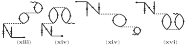
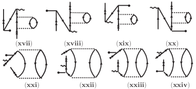
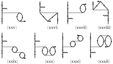
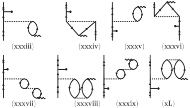
Figure 2: A few important electron correlation contributing diagrams to $E1_{PV}$ in the RMBPT(3) method. The dotted lines represent the atomic Hamiltonian. Diagrams (i)-(viii) give Core contributions in the RMBPT(3)^w method, but they correspond to Valence contributions in the RMBPT(3)^d method. Diagrams (ix)-(xvi) follow other way around.

III.1 Sum-over-states approach

In the sum-over-states approach, the first-order wave function of a general state can be expressed as

$$|\Psi_{v}^{(1)}\rangle = \sum_{I\neq v}|\Psi_{I}^{(0)}\rangle\frac{\langle\Psi_{I}^{(0)}|H_{W}|\Psi_{v}^{(0)}\rangle}{{\cal N}_{v}(E_{v}^{(0)}-E_{I}^{(0)})},$$ (21)

where $|\Psi_{I}^{(0)}\rangle$ are the zeroth-order intermediate states and $E_{n}^{(0)}$ is the unperturbed energy of the $n^{th}$ level. Thus, Eq. (15) can be written as

$$E1_{PV} = \sum_{I\neq i}\frac{\langle\Psi_{f}^{(0)}|D|\Psi_{I}^{(0)}\rangle\langle\Psi_{I}^{(0)}|H_{W}|\Psi_{i}^{(0)}\rangle}{{\cal N}_{if}(E_{i}^{(0)}-E_{I}^{(0)})}$$ (22)

$$+\sum_{I\neq f}\frac{\langle\Psi_{f}^{(0)}|H_{W}|\Psi_{I}^{(0)}\rangle\langle\Psi_{I}^{(0)}|D|\Psi_{i}^{(0)}\rangle}{{\cal N}_{if}(E_{f}^{(0)}-E_{I}^{(0)})}.$$

In the above expression of $E1_{PV}$, correlations among the $H$ and $H_{W}$ that appear through Eq. (17) are omitted. Secondly, there could be conflict with the definitions of using Core, Main and Tail contributions to $E1_{PV}$ with the definitions used in various first-principle based calculations. This is explicitly demonstrated later how formula given by Eq. (20) can be altered to redefine Core and Valence contributions. To understand definitions of Core, Main and Tail contributions used in Ref. [24], we follow the work of Blundell et al [12] where these terms were used for the first time in the context of estimating $E1_{PV}$. Division of the total $E1_{PV}$ value in this calculation was made as “Main”, “Core” and “Tail” contributions based on the mere assumption that $|\Psi_{i}^{(0)}\rangle$, $|\Psi_{f}^{(0)}\rangle$ and $|\Psi_{I}^{(0)}\rangle$ are represented by only single Slater determinants like in the DHF method. Thus, the intermediate states $|\Psi_{I}^{(0)}\rangle$ are considered to have only the $np~{}^{2}P_{1/2}$ configurations. In such assumption, the Core ($C$), Main ($V$) and Tail ($T$) contributions to the $E1_{PV}$ amplitude of the $6s~{}^{2}S_{1/2}-7s~{}^{2}S_{1/2}$ transition in ¹³³Cs were estimated as

$$E1_{PV}(C) = \sum_{n\leq 5}\frac{\langle 7S_{1/2}|D|nP_{1/2}\rangle\langle nP_{1/2}|H_{W}|6S_{1/2}\rangle}{(E_{6S_{1/2}}-E_{nP_{1/2}})}$$ (23)

$$+ \sum_{n\leq 5}\frac{\langle 7S_{1/2}|H_{W}|nP_{1/2}\rangle\langle nP_{1/2}|D|6S_{1/2}\rangle}{(E_{7S_{1/2}}-E_{nP_{1/2}})}\ \ \$$

$$E1_{PV}(V) = \sum_{n=6-9}\frac{\langle 7S_{1/2}|D|nP_{1/2}\rangle\langle nP_{1/2}|H_{W}|6S_{1/2}\rangle}{(E_{6S_{1/2}}-E_{nP_{1/2}})}$$ (24)

$$+ \sum_{n=6-9}\frac{\langle 7S_{1/2}|H_{W}|nP_{1/2}\rangle\langle nP_{1/2}|D|6S_{1/2}\rangle}{(E_{7S_{1/2}}-E_{nP_{1/2}})}\ \ \$$

and

$$E1_{PV}(T) = \sum_{n\geq 10}\frac{\langle 7S_{1/2}|D|nP_{1/2}\rangle\langle nP_{1/2}|H_{W}|6S_{1/2}\rangle}{(E_{6S_{1/2}}-E_{nP_{1/2}})}$$ (25)

$$+ \sum_{n\geq 10}\frac{\langle 7S_{1/2}|H_{W}|nP_{1/2}\rangle\langle nP_{1/2}|D|6S_{1/2}\rangle}{(E_{7S_{1/2}}-E_{nP_{1/2}})},\ \ \$$

respectively. However, wave functions of multi-electron atomic systems are determined through a many-body method by expressing as a linear combination of many Slater determinants which can differ by either single or multiple entries of rows or columns. As a result, contributions from cross-terms involving other Slater determinants, e.g. excited configurations $5p^{5}6s7s$ of the intermediate states with respect to both the $6s~{}^{2}S_{1/2}$ and $7s~{}^{2}S_{1/2}$ states, cannot appear through the above breakup. One of such contributions is referred to as DCP effects which arise through the CPDF-RPA (or TDHF) method as described by Mårtensson [11] and Roberts [26]. There are other contributions that could come through effects that are neither part of BO contributions nor CPDF-RPA method. However those effects appear through the first-principle approach of the RCC method employed by Sahoo et al [32] as shown later part of this paper. These contributions are not small and demands for an appropriate many-body method to account their contributions at the par with the $np~{}^{2}P_{1/2}$ intermediate states. This argument can be understood better with the following explanations.

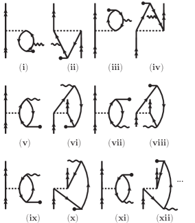
Figure 3: A few representative DCP diagrams from the RMBPT(3) method. All-order forms of diagrams from (i) to (viii) appear in the CPDF-RPA method, but the rest are not. These missing contributions appear in the RCC theory to all-orders.

In the ¹³³Cs atom, the low-lying excited states have a common core $[5p^{6}]$ and differ by only a valence orbital. Thus, the DHF wave functions of these states can be expressed as $|\Phi_{I}\rangle=a_{I}^{\dagger}|\Phi_{0}\rangle$ and the exact wave functions can be defined as

$$|\Psi_{I}^{(0)}\rangle = \Omega^{I(0)}|\Phi_{I}\rangle$$ (26)

$$= (\Omega_{0}^{(0)}+\Omega_{I}^{(0)})|\Phi_{I}\rangle,$$

where $\Omega^{I(0)}$ and $\Omega_{I}^{(0)}$ are the total and valence correlation contributing wave operators respectively. Using these wave operators, we can express Eq. (22) as

$$E1_{PV} = \sum_{I\neq i}\frac{\langle\Phi_{0}|a_{f}(\Omega_{0}^{(0)}+\Omega_{f}^{(0)})^{\dagger}D(\Omega_{0}^{(0)}+\Omega_{I}^{(0)})a_{I}^{\dagger}|\Phi_{0}\rangle}{{\cal N}_{if}}$$ (27)

$$\times \frac{\langle\Phi_{0}|a_{I}(\Omega_{0}^{(0)}+\Omega_{I}^{(0)})^{\dagger}H_{W}(\Omega_{0}^{(0)}+\Omega_{i}^{(0)})a_{i}^{\dagger}|\Phi_{0}\rangle}{(E_{i}^{(0)}-E_{I}^{(0)})}$$

$$+ \sum_{I\neq f}\frac{\langle\Phi_{0}|a_{f}(\Omega_{0}^{(0)}+\Omega_{f}^{(0)})^{\dagger}H_{W}(\Omega_{0}^{(0)}+\Omega_{I}^{(0)})a_{I}^{\dagger}|\Phi_{0}\rangle}{{\cal N}_{if}}$$

$$\times \frac{\langle\Phi_{0}|a_{I}(\Omega_{0}^{(0)}+\Omega_{I}^{(0)})^{\dagger}D(\Omega_{0}^{(0)}+\Omega_{i}^{(0)})a_{i}^{\dagger}|\Phi_{0}\rangle}{(E_{f}^{(0)}-E_{I}^{(0)})}.$$

Since wave operators from the initial, final and intermediate states include linear combinations of configurations describing one-hole–one-particle, two-hole–two-particle etc. excitations, it is obvious that a sum-over-states approach cannot include contributions from the higher-level excited configurations contributing to the intermediate states.

III.2 First-principle approach

It is evident that it is imperative to determine the $E1_{PV}$ amplitudes in atomic systems using the first principle approaches that account contributions from all possible intermediate configurations. This can be done using either Eq. (15) or Eq. (20). It is desirable to solve both Eqs. (16) and (17) in the former case, while Bloch’s equations for the unperturbed and perturbed wave operators need to be solved for the later approach. The amplitude solving Bloch’s equations for the unperturbed operators $\Omega_{0}^{(0)}$ and $\Omega_{v}^{(0)}$ are similar to that are given by Eqs. (9) and (10), respectively. The Bloch’s equations for the first-order perturbed wave operators can be given by

$$[\Omega_{0}^{(1)},H_{0}]P_{0} = (H_{W}\Omega_{0}^{(0)}+U_{res}\Omega_{0}^{(1)})P_{0}$$ (28)

and

$$[\Omega_{v}^{(1)},H_{0}]P_{v} = [H_{W}(\Omega_{0}^{(0)}+\Omega_{v}^{(0)})+U_{res}(\Omega_{0}^{(1)}+\Omega_{v}^{(1)})P_{v}$$ (29)

$$-\Omega_{v}^{(1)}E_{v}^{(0)}.$$

As mentioned in Introduction, several all-order methods in the CPDF, RPA, CPDF-RPA/TDHF and RCC theory frameworks are employed to determine the $E1_{PV}$ amplitudes in ¹³³Cs. Here, we attempt to formulate all these methods using wave operators so that in the end it would be easier for us to make one-to-one relations among various contributions arising through these methods. Especially, such exercise is going to be useful in explaining the reason for which there is a sign difference between the Core contributions to $E1_{PV}$ from the TDHF method of Dzuba et al [25] and RCC method employed by Sahoo et al [29].

We can rewrite Eq. (15) as

$$E1_{PV}=\frac{\langle\Psi_{f}^{(0)}|H_{W}|\tilde{\Psi}_{i}^{(1)}\rangle}{{\cal N}_{if}}+\frac{\langle\tilde{\Psi}_{f}^{(1)}|H_{W}|\Psi_{i}^{(0)}\rangle}{{\cal N}_{if}}.$$ (30)

This can be equivalently expressed by either

$$E1_{PV} = \frac{\langle\Psi_{f}^{(0)}|D|\Psi_{i}^{(1)}\rangle}{{\cal N}_{if}}+\frac{\langle\Psi_{f}^{(0)}|H_{W}|\tilde{\Psi}_{i}^{(1)}\rangle}{{\cal N}_{if}}$$ (31)

or

$$E1_{PV} = \frac{\langle\tilde{\Psi}_{f}^{(1)}|H_{W}|\Psi_{i}^{(0)}\rangle}{{\cal N}_{if}}+\frac{\langle\Psi_{f}^{(1)}|D|\Psi_{i}^{(0)}\rangle}{{\cal N}_{if}}.$$ (32)

In the above expressions, we define

$$|\tilde{\Psi}_{i}^{(1)}\rangle = \sum_{I\neq f}|\Psi_{I}^{(0)}\rangle\frac{\langle\Psi_{I}^{(0)}|D|\Psi_{i}^{(0)}\rangle}{(E_{i}^{(0)}-E_{I}^{(0)}+\omega)}$$ (33)

and

$$|\tilde{\Psi}_{f}^{(1)}\rangle = \sum_{I\neq i}|\Psi_{I}^{(0)}\rangle\frac{\langle\Psi_{I}^{(0)}|D|\Psi_{f}^{(0)}\rangle}{(E_{f}^{(0)}-E_{I}^{(0)}-\omega)}$$ (34)

with $\omega=E_{f}^{(0)}-E_{i}^{(0)}$ is the excitation energy between the initial and final states. It implies that mathematically Eqs. (15), (30), (31) and (32) are equal in an exact many-body method. Thus, any of these expressions can be used in the determination of the $E1_{PV}$ amplitude. We shall demonstrate later that the CPDF, RPA, CPDF-RPA and RCC methods are using different formulas as mentioned above. So it is important to understand their relations and classifications of individual contributions through the above methods. Since approximations made to the unperturbed and perturbed wave functions are not at the same level in these methods, it is obvious to guess that results from these methods can be very different unless electron correlation effects in an atomic system are negligibly small. It is also not clear whether classifications of Core and Tail contributions in these methods are uniquely defined or not.

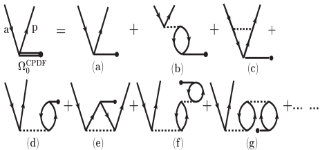
Figure 4: Goldstone diagrams contributing to amplitude determining equation of $\Omega_{0}^{CPDF}$. Through iterative scheme these effects are included to all-orders in the CPDF method.

To understand the above points, lets find out the Core contributions from Eqs. (15) and (30) by expressing the perturbed wave function due to the $D$ operator in terms of wave operators as

$$|\tilde{\Psi}_{v}^{(1)}\rangle=(\tilde{\Omega}_{0}^{(1)}+\tilde{\Omega}_{v}^{(1)})|\Phi_{v}\rangle.$$ (35)

With this, the Core contributing terms in both $H_{W}$ and $D$ perturbing approaches are given by

$$E1_{PV}(C) = \frac{\langle\Phi_{0}|a_{f}[\Omega_{0}^{(0)\dagger}D\Omega_{0}^{(1)}+\Omega_{0}^{(1)\dagger}D\Omega_{0}^{(0)}]a_{i}^{\dagger}|\Phi_{0}\rangle}{{\cal N}_{if}}\ \ \$$ (36)

and

$$E1_{PV}(C) = \frac{\langle\Phi_{0}|a_{f}[\tilde{\Omega}_{0}^{(1)\dagger}H_{W}\Omega_{0}^{(0)}+\Omega_{0}^{(0)\dagger}H_{W}\tilde{\Omega}_{0}^{(1)}]a_{i}^{\dagger}|\Phi_{0}\rangle}{{\cal N}_{if}}.\ \ \$$ (37)

After a careful analysis it can be shown that the Core contributions arising through the wave operators $\Omega_{0}^{(1)}$ and $\tilde{\Omega}_{0}^{(1)}$ can be different. Similar arguments also hold for the Tail contributions arising through the perturbed valence operators $\Omega_{v}^{(1)}$ and $\tilde{\Omega}_{v}^{(1)}$. To get better inside of this argument, we can rewrite the sum-over-states formula given by Eq. (27) as

$$E1_{PV} = \sum_{I\neq i}\frac{\langle\Phi_{0}|a_{f}\Omega_{0}^{(0)\dagger}D\Omega_{0}^{(0)}\Omega_{0}^{(0)\dagger}H_{W}\Omega_{0}^{(0)}a_{i}^{\dagger}|\Phi_{0}\rangle}{{\cal N}_{if}(E_{f}^{(0)}-E_{I}^{(0)}-\omega)}$$

$$+ \sum_{I\neq i}\frac{\langle\Phi_{0}|a_{f}\Omega_{f}^{(0)\dagger}D\Omega_{0}^{(0)}\Omega_{0}^{(0)\dagger}H_{W}\Omega_{i}^{(0)}a_{i}^{\dagger}|\Phi_{0}\rangle}{{\cal N}_{if}(E_{f}^{(0)}-E_{I}^{(0)}-\omega)}$$

$$+ \sum_{I\neq i}\frac{\langle\Phi_{0}|a_{f}\Omega_{0}^{(0)\dagger}D\Omega_{0}^{(0)}\Omega_{0}^{(0)\dagger}H_{W}\Omega_{i}^{(0)}a_{i}^{\dagger}|\Phi_{0}\rangle}{{\cal N}_{if}(E_{f}^{(0)}-E_{I}^{(0)}-\omega)}$$

$$+ \sum_{I\neq i}\frac{\langle\Phi_{0}|a_{f}\Omega_{f}^{(0)\dagger}D\Omega_{0}^{(0)}\Omega_{0}^{(0)\dagger}H_{W}\Omega_{0}^{(0)}a_{i}^{\dagger}|\Phi_{0}\rangle}{{\cal N}_{if}(E_{f}^{(0)}-E_{I}^{(0)}-\omega)}$$

$$+ \sum_{I\neq i}\frac{\langle\Phi_{0}|a_{f}\Omega_{0}^{(0)\dagger}D\Omega_{I}^{(0)}\Omega_{I}^{(0)\dagger}H_{W}\Omega_{0}^{(0)}a_{i}^{\dagger}|\Phi_{0}\rangle}{{\cal N}_{if}(E_{f}^{(0)}-E_{I}^{(0)}-\omega)}$$

$$+ \sum_{I\neq i}\frac{\langle\Phi_{0}|a_{f}\Omega_{f}^{(0)\dagger}D\Omega_{I}^{(0)}\Omega_{I}^{(0)\dagger}H_{W}\Omega_{i}^{(0)}a_{i}^{\dagger}|\Phi_{0}\rangle}{{\cal N}_{if}(E_{f}^{(0)}-E_{I}^{(0)}-\omega)}$$

$$+ \sum_{I\neq i}\frac{\langle\Phi_{0}|a_{f}\Omega_{0}^{(0)\dagger}D\Omega_{I}^{(0)}\Omega_{I}^{(0)\dagger}H_{W}\Omega_{i}^{(0)}a_{i}^{\dagger}|\Phi_{0}\rangle}{{\cal N}_{if}(E_{f}^{(0)}-E_{I}^{(0)}-\omega)}$$

$$+ \sum_{I\neq i}\frac{\langle\Phi_{0}|a_{f}\Omega_{f}^{(0)\dagger}D\Omega_{I}^{(0)}\Omega_{I}^{(0)\dagger}H_{W}\Omega_{0}^{(0)}a_{i}^{\dagger}|\Phi_{0}\rangle}{{\cal N}_{if}(E_{f}^{(0)}-E_{I}^{(0)}-\omega)}$$

$$+ \sum_{I\neq i}\frac{\langle\Phi_{0}|a_{f}\Omega_{0}^{(0)\dagger}D\Omega_{I}^{(0)}\Omega_{0}^{(0)\dagger}H_{W}\Omega_{0}^{(0)}a_{i}^{\dagger}|\Phi_{0}\rangle}{{\cal N}_{if}(E_{f}^{(0)}-E_{I}^{(0)}-\omega)}$$

$$+ \sum_{I\neq i}\frac{\langle\Phi_{0}|a_{f}\Omega_{f}^{(0)\dagger}D\Omega_{I}^{(0)}\Omega_{0}^{(0)\dagger}H_{W}\Omega_{i}^{(0)}a_{i}^{\dagger}|\Phi_{0}\rangle}{{\cal N}_{if}(E_{f}^{(0)}-E_{I}^{(0)}-\omega)}$$

$$+ \sum_{I\neq i}\frac{\langle\Phi_{0}|a_{f}\Omega_{0}^{(0)\dagger}D\Omega_{I}^{(0)}\Omega_{0}^{(0)\dagger}H_{W}\Omega_{i}^{(0)}a_{i}^{\dagger}|\Phi_{0}\rangle}{{\cal N}_{if}(E_{f}^{(0)}-E_{I}^{(0)}-\omega)}$$

$$+ \sum_{I\neq i}\frac{\langle\Phi_{0}|a_{f}\Omega_{f}^{(0)\dagger}D\Omega_{I}^{(0)}\Omega_{0}^{(0)\dagger}H_{W}\Omega_{0}^{(0)}a_{i}^{\dagger}|\Phi_{0}\rangle}{{\cal N}_{if}(E_{f}^{(0)}-E_{I}^{(0)}-\omega)}$$

$$+ \sum_{I\neq i}\frac{\langle\Phi_{0}|a_{f}\Omega_{0}^{(0)\dagger}D\Omega_{0}^{(0)}\Omega_{I}^{(0)\dagger}H_{W}\Omega_{0}^{(0)}a_{i}^{\dagger}|\Phi_{0}\rangle}{{\cal N}_{if}(E_{f}^{(0)}-E_{I}^{(0)}-\omega)}$$

$$+ \sum_{I\neq i}\frac{\langle\Phi_{0}|a_{f}\Omega_{f}^{(0)\dagger}D\Omega_{0}^{(0)}\Omega_{I}^{(0)\dagger}H_{W}\Omega_{i}^{(0)}a_{i}^{\dagger}|\Phi_{0}\rangle}{{\cal N}_{if}(E_{f}^{(0)}-E_{I}^{(0)}-\omega)}$$

$$+ \sum_{I\neq i}\frac{\langle\Phi_{0}|a_{f}\Omega_{0}^{(0)\dagger}D\Omega_{0}^{(0)}\Omega_{I}^{(0)\dagger}H_{W}\Omega_{i}^{(0)}a_{i}^{\dagger}|\Phi_{0}\rangle}{{\cal N}_{if}(E_{f}^{(0)}-E_{I}^{(0)}-\omega)}$$

$$+ \sum_{I\neq i}\frac{\langle\Phi_{0}|a_{f}\Omega_{f}^{(0)\dagger}D\Omega_{0}^{(0)}\Omega_{I}^{(0)\dagger}H_{W}\Omega_{0}^{(0)}a_{i}^{\dagger}|\Phi_{0}\rangle}{{\cal N}_{if}(E_{f}^{(0)}-E_{I}^{(0)}-\omega)}$$

$$+ \{H_{W}\Leftrightarrow D\}$$

Both Eqs. (27) and Eq. (LABEL:eq60) are equal but they are given differently. These equations are nothing but the expanded forms of Eqs. (20) and (30) respectively. However, different terms are rearranged to place them under the categories of Core and Valence contributing terms in the respective formulas. Thus, we may now outline findings from the above discussions as follows

1. It is important to note that in the evaluation of $E1_{PV}$ both the $H_{W}$ and $D$ operators can be treated symmetrically. Thus, in an approximated method where correlation effects through both these operators are not incorporated equivalently, distinctions of “Core” and “Valence” contributions to $E1_{PV}$ cannot be defined uniquely.

2. As a consequence of the above point, estimating both the “Core” and “Valence” contributions using a blend of many-body methods could mislead the final result.

3. Numerical stability to the calculation of $E1_{PV}$ can be verified by evaluating expressions given by Eqs. (15), (30) and (31) simultaneously though it can be a strenuous procedure.

4. Scaling wave functions for estimating a part of contribution or using experimental value of $\omega$ in an approximated method may not always imply that the result is improved rather it could introduce further uncertainty to the calculation.

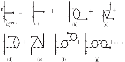
Figure 5: Diagrams denoting amplitude solving equation for $\Omega_{v}^{CPDF}$. These core-polarization effects are included to all-orders in the CPDF method.

The last point mentioned above can be understood as discussed below. Lets use the experimental value for $\omega$ (shown as $\omega^{ex}$) to define the first-order perturbed wave functions due to the $D$ operator

$$|\tilde{\Psi}_{i}^{(1)}\rangle = \sum_{I\neq f}|\Psi_{I}^{(0)}\rangle\frac{\langle\Psi_{I}^{(0)}|D|\Psi_{i}^{(0)}\rangle}{(E_{i}^{(0)}-E_{I}^{(0)}+\omega^{ex})}$$ (39)

and

$$|\tilde{\Psi}_{f}^{(1)}\rangle = \sum_{I\neq i}|\Psi_{I}^{(0)}\rangle\frac{\langle\Psi_{I}^{(0)}|D|\Psi_{f}^{(0)}\rangle}{(E_{f}^{(0)}-E_{I}^{(0)}-\omega^{ex})}.$$ (40)

Substituting these wave functions in Eq. (22), the sum-over-states expression for $E1_{PV}$ can be given by

$$E1_{PV} = \sum_{I\neq i}\frac{\langle\Psi_{f}^{(0)}|D|\Psi_{I}^{(0)}\rangle\langle\Psi_{I}^{(0)}|H_{W}|\Psi_{i}^{(0)}\rangle}{{\cal N}_{if}(E_{i}^{(0)}-E_{I}^{(0)}-\delta\omega)}$$ (41)

$$+\sum_{I\neq f}\frac{\langle\Psi_{f}^{(0)}|H_{W}|\Psi_{I}^{(0)}\rangle\langle\Psi_{I}^{(0)}|D|\Psi_{i}^{(0)}\rangle}{{\cal N}_{if}(E_{f}^{(0)}-E_{I}^{(0)}+\delta\omega)},$$

where $\delta\omega=\omega^{ex}-\omega$, with $\omega$ being the theoretical value, cannot be zero when $\omega$ is obtained using a particular many-body method. As can be seen, introduction of $\omega^{ex}$ value affects contributions from the initial and final perturbed terms differently leading to inconsistency in the evaluation of $E1_{PV}$ than the ab initio calculation. This can be better evident from the following inequalities in an approximated many-body method

$$E1_{PV} = \frac{\langle\Psi_{f}^{(0)}|D|\Psi_{i}^{(1)}\rangle}{{\cal N}_{if}}+\frac{\langle\Psi_{f}^{(1)}|D|\Psi_{i}^{(0)}\rangle}{{\cal N}_{if}}$$ (42)

$$\neq \frac{\langle\Psi_{f}^{(0)}|H_{W}|\tilde{\Psi}_{i}^{(1)}\rangle}{{\cal N}_{if}}+\frac{\langle\tilde{\Psi}_{f}^{(1)}|H_{W}|\Psi_{i}^{(0)}\rangle}{{\cal N}_{if}}$$

$$\neq \frac{\langle\Psi_{f}^{(0)}|D|\Psi_{i}^{(1)}\rangle}{{\cal N}_{if}}+\frac{\langle\Psi_{f}^{(0)}|H_{W}|\tilde{\Psi}_{i}^{(1)}\rangle}{{\cal N}_{if}}$$

$$\neq \frac{\langle\tilde{\Psi}_{f}^{(1)}|H_{W}|\Psi_{i}^{(0)}\rangle}{{\cal N}_{if}}+\frac{\langle\Psi_{f}^{(1)}|D|\Psi_{i}^{(0)}\rangle}{{\cal N}_{if}}.$$

The above inequalities are the result of introduction of $\delta\omega$ in the first-order perturbed wave function due to $D$ after the substitution of $\omega^{ex}$ in place of $\omega$.

IV Many-body methods of $E1_{PV}$

The main objective in the APV study is to obtain the $E1_{PV}$ amplitude within sub-one percent accuracy from the atomic many-body theory perspective. In view of this, it is imperative to evaluate both the zeroth-order and first-order atomic wave functions in Eq. (15) very accurately by employing a powerful relativistic atomic many-body method. Owing to complications in accounting for various contributions, the entire calculation is usually performed in several steps. The majority of the contribution from $H$ arises from electron correlation effects due to Coulomb interactions in the presence of APV interactions, while corrections from the Breit and QED interactions are added separately. It would be necessary to include all these interactions through a common many-body theory in order to consider correlations among themselves as well. Since corrections from the Breit and QED interactions to $E1_{PV}$ are very small, their reported estimations are found to be almost consistent to each other by various works [14, 15, 16, 17, 18, 19, 20, 32]. Thus, we focus here mainly on the discussions considering the Dirac-Coulomb (DC) interaction Hamiltonian in the determination of unperturbed wave functions. Again, our aim in the present paper is to demonstrate how to achieve high-accuracy calculations of the $E1_{PV}$ amplitudes in ¹³³Cs by understanding about the roles of Core correlations to these quantities and identifying contributions that can arise through a particular many-body method but can be missed by another method. To explain these points explicitly, we discuss calculations of the $E1_{PV}$ amplitudes in ¹³³Cs using the following methods

1. Relativistic Many-body Perturbation Theory (RMBPT): This method is employed in the Rayleigh-Schrödinger perturbation theory framework to fathom about significance of various physical effects to $E1_{PV}$ arising at the lower-order level and to learn how they propagate in the all-order perturbative methods.

2. CPDF method: This method is employed in order to reproduce previous results reported by other groups using the same method using our basis functions that are later considered in the RCC calculations.

3. RPA: This method is employed for the same purpose as the above and show importance of correlation contributions arising through this method which are missing in the CPDF method.

4. CPDF-RPA method: This method is employed again for the above purpose as well as understanding the reason for which Core contribution from Ref. [25] has a different sign than other works.

5. RCC method: This method is employed both in the sum-over-states and first-principle approaches. Differences in both the results are further compared with the values that are included through the CPDF-RPA method.

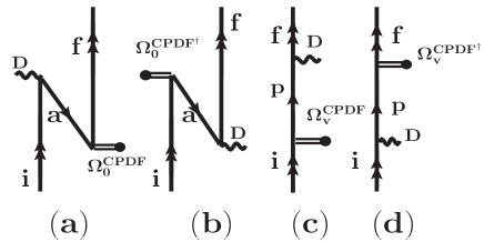
Figure 6: Property diagrams of the CPDF method. These diagrams are similar to the DHF method, but the $H_{W}$ operators of the DHF diagrams are replaced by $\Omega_{0}^{CPDF}$ and $\Omega_{v}^{CPDF}$. Expansion of $\Omega_{0}^{CPDF}$ and $\Omega_{v}^{CPDF}$ in terms of amplitude diagrams shown in Figs. 4 and 5 can reveal how the DHF contributions and lower-order core-polarization effects of the RMBPT(3) method are incorporated within the CPDF method.

The atomic Hamiltonian H with DC approximation can be expressed as sum of one-body and two-body operators

$$H = \sum_{i}\left[c\mbox{\boldmath${\vec{\alpha}}$}^{D}\cdot{\vec{p}}_{i}+(\beta-1)c^{2}+V_{nuc}(r_{i})\right]+\sum_{i,j>i}\frac{1}{r_{ij}}$$ (43)

$$= \sum_{i}h(r_{i})+\sum_{i,j>i}g(r_{ij}),$$

where $c$ is the speed of light, $\mbox{\boldmath${\vec{\alpha}}$}^{D}$ and $\beta$ are the Dirac matrices, ${\vec{p}}$ is the single particle momentum operator, and $\sum_{i,j}\frac{1}{r_{ij}}$ represents the Coulomb potential between the electrons located at the $i^{th}$ and $j^{th}$ positions. The entire Hamiltonian can be divided into one-body part ($\sum_{i}h(r_{i})$) and two-body part ($\sum_{i,j>i}g(r_{ij})$) for convenience. Using the DHF method, we can obtain the single particle orbitals using the modified DHF Hamiltonian as $F=\sum_{i}f(r_{i})=\sum_{i}(h_{i}+u_{i}^{(0)})$ and residual interaction as $V_{res}=H-F$ in the DC approximation. Hence

$$f|i\rangle=\epsilon_{i}|i\rangle$$ (44)

with the single particle energies $\epsilon_{i}$ giving unperturbed DHF energy ${\cal E}_{0}=\sum_{b}^{N_{c}}\epsilon_{b}$ and the DHF potential $U_{DHF}=\sum_{i}u_{0}(r_{i})$ is given by

$$u_{0}(r_{i})|i\rangle=\sum_{b}^{N_{c}}\left[\langle b|g|b\rangle|i\rangle-\langle b|g|i\rangle|b\rangle\right]$$ (45)

for $b$ summing over all occupied-orbitals $N_{c}$. In the DHF method, both Eqs. (44) and (45) are solved iteratively to obtain self-consistent solutions. It can be followed from the above expression that for the determinant expressed by $|\Phi_{k}\rangle=a_{k}^{\dagger}|\Phi_{0}\rangle$, the DHF energy is given by ${\cal E}_{k}={\cal E}_{0}+\epsilon_{k}$. Similarly, DHF energies of the excited configurations are given by ${\cal E}_{a,b,\cdots}^{p,q,\cdots}={\cal E}_{0}+\epsilon_{p}+\epsilon_{p}+\cdots-\epsilon_{a}-\epsilon_{b}-\cdots$ where $\{a,b,\cdots\}$ and $\{p,q,\cdots\}$ denoting for the occupied and unoccupied orbitals respectively. We discuss below $E1_{PV}$ expressions using the DHF method and different many-body methods that are employed to account for the electron correlation effects due to $V_{res}$.

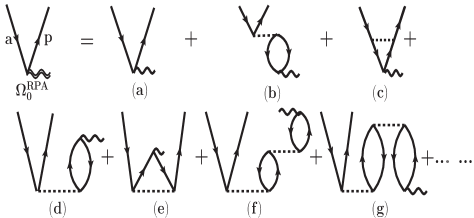
Figure 7: Graphical representation of $\Omega_{0}^{RPA}$ and its expansion in terms of lower-order RMBPT(3) method.

IV.1 DHF method

Using wave functions from the DHF method, we can evaluate the $E1_{PV}$ amplitude in the mean-field approach as

$$E1_{PV}=\langle\Phi_{f}|D|\Phi_{i}^{(1)}\rangle+\langle\Phi_{f}^{(1)}|D|\Phi_{i}\rangle,$$ (46)

where $|\Phi_{n=i,f}^{(1)}\rangle$ is the first-order perturbed wave function with respect to $|\Phi_{n=i,f}\rangle$. We can express these wave function as

$$|\Phi_{n}^{(1)}\rangle=\sum_{I}|\Phi_{I}\rangle\frac{\langle\Phi_{I}|H_{W}|\Phi_{n}\rangle}{{\cal E}_{n}-{\cal E}_{I}},$$ (47)

where $|\Phi_{I}\rangle$ are the intermediate states with mean-field energies ${\cal E}_{I}$. Substituting this expression above, it yields

$$E1_{PV} = \sum_{I\neq i}\frac{\langle\Phi_{f}|D|\Phi_{I}\rangle\langle\Phi_{I}|H_{W}|\Phi_{i}\rangle}{{\cal E}_{i}-{\cal E}_{I}}$$ (48)

$$+\sum_{I\neq f}\frac{\langle\Phi_{f}|H_{W}|\Phi_{I}\rangle\langle\Phi_{I}|D|\Phi_{i}\rangle}{{\cal E}_{f}-{\cal E}_{I}}.$$

Using $H_{W}=\sum_{i}h_{w}(r_{i})$ and $D=\sum_{i}d(r_{i})$, and following the Slater-Condon rules, it gives

$$E1_{PV} = \sum_{a}\frac{\langle f|d|a\rangle\langle a|h_{w}|i\rangle}{\epsilon_{i}-\epsilon_{a}}+\sum_{a}\frac{\langle f|h_{w}|a\rangle\langle a|d|i\rangle}{\epsilon_{f}-\epsilon_{a}}$$ (49)

$$+ \sum_{p\neq i}\frac{\langle f|d|p\rangle\langle p|h_{w}|i\rangle}{\epsilon_{i}-\epsilon_{p}}+\sum_{p\neq f}\frac{\langle f|h_{w}|p\rangle\langle p|d|i\rangle}{\epsilon_{f}-\epsilon_{p}},\ \ \ \$$

where $|k=a,p\rangle$ denotes $k^{th}$ single particle DHF orbital with energy $\epsilon_{k}$ for the occupied orbitals denoted by $a$ and virtual orbitals denoted by $p$. Contributions arising from the first two terms of the above expression are referred to as the lowest-order Core contributions while contributions from the later two terms are said to be Valence contributions that include the lowest-orders to both Main and Tail parts.

In terms of wave operators, the DHF expression for $E1_{PV}$ can be given by

$$E1_{PV}=\langle\Phi_{f}|D\Omega^{i(0,1)}|\Phi_{i}\rangle+\langle\Phi_{f}|\Omega^{f(0,1)\dagger}D|\Phi_{i}\rangle,$$ (50)

where $\Omega^{v(0,1)}=\Omega_{0}^{(0,1)}+\Omega_{v}^{(0,1)}$. For single excitations, $\Omega_{0}^{(0,1)}\rightarrow\Omega_{1}^{(0,1)}=\sum_{a,p}\frac{\langle\Phi_{a}^{p}|H_{W}|\Phi_{0}\rangle}{{\cal E}_{0}-{\cal E}_{a}^{p}}a_{p}^{\dagger}a_{a}=\sum_{a,p}\frac{\langle p|h_{w}|a\rangle}{\epsilon_{a}-\epsilon_{p}}a_{p}^{\dagger}a_{a}\equiv\sum_{a,p}\Omega_{a}^{p}$ and $\Omega_{v}^{(0,1)}\rightarrow\Omega_{1v}^{(0,1)}=\sum_{p}\frac{\langle\Phi_{v}^{p}|H_{W}|\Phi_{v}\rangle}{{\cal E}_{v}-{\cal E}_{v}^{p}}a_{p}^{\dagger}a_{v}=\frac{\langle p|h_{w}|v\rangle}{\epsilon_{v}-\epsilon_{p}}a_{p}^{\dagger}a_{a}\equiv\sum_{p}\Omega_{v}^{p}$ for the intermediate states $|\Phi_{a}^{p}\rangle$ with energies ${\cal E}_{a}^{p}={\cal E}_{0}+\epsilon_{p}-\epsilon_{a}$ and $|\Phi_{v}^{p}\rangle$ with energies ${\cal E}_{v}^{p}={\cal E}_{0}+\epsilon_{p}$ with respect to the $|\Phi_{0}\rangle$ and $|\Phi_{v}\rangle$ respectively. It should be noted that for double excitations $\Omega_{0}^{(0,1)}\rightarrow\Omega_{2}^{(0,1)}=0$ and $\Omega_{v}^{(0,1)}\rightarrow\Omega_{2v}^{(0,1)}=0$. Representing the wave operators in terms of the Goldstone diagrams, we show the Core and Valence contributions to $E1_{PV}$ in Fig. 1. Figs. 1(a) and (b) correspond to Core contributing terms, while Figs. 1(c) and (d) correspond to Valence contributing terms here.

Figure 8: Graphical representation of $\Omega_{v}^{RPA}$ and its expansion in terms of lower-order RMBPT(3) method.

IV.2 RMBPT method

We employ the RMBPT method in the Rayleigh-Schrödinger approach and estimate contributions only up to third-order of perturbation (RMBPT(3) method) by considering two orders of $V_{res}$ and one-order of $H_{W}$; i.e. the net Hamiltonian is expressed as

$$H_{at}=F+\lambda_{1}V_{res}+\lambda_{2}H_{W},$$ (51)

where $\lambda_{1}$ and $\lambda_{2}$ are arbitrary parameters introduced to count orders of $V_{res}$ and $H_{W}$ in the calculation. Here, we can calculate either matrix element of $D$ after perturbing wave functions by $H_{W}$ or matrix element of $H_{W}$ after perturbing wave functions by $D$. We adopt here both approaches for two reasons. First, it can help us to identify the lower-order contributions terms to the CPDF and RPA methods so that their inclusion through the RCC method can be easily understood. Second, it would be interesting to see classification of the Core and Valence contributions in both the approaches of the RMBPT method. In both the approaches, the unperturbed wave operators in the RMBPT method can be given by

$$\Omega_{n}^{(0)}=\sum_{k}\Omega_{n}^{(k,0)}.$$ (52)

Similarly, the first-order perturbed wave operators can be denoted by

$$\Omega_{n}^{(1)}=\sum_{k}\Omega_{n}^{(k,1)},$$ (53)

where subscript $n=0,v$ stands for core or valence operators and superscript $k$ denotes for order of $V_{res}$. Amplitudes of the wave operators in the RMBPT method are determined by

$$[\Omega_{0}^{(k,0)},F]P_{0} = Q_{0}V_{res}\Omega_{0}^{(k-1,0)}P_{0}$$ (54)

and

$$[\Omega_{v}^{(k,0)},F]P_{v} = Q_{v}V_{res}(\Omega_{0}^{(k-1,0)}+\Omega_{v}^{(k-1,0)})P_{v}$$ (55)

$$-\sum_{m=1}^{k-1}\Omega_{v}^{(k-m,0)}E_{v}^{(m,0)},$$

where $E_{v}^{(m,0)}$ is the $m^{th}$-order perturbed energy of the total energy $E_{v}^{(0)}=\sum_{m=1}^{\infty}E_{v}^{(m,0)}$ and is evaluated by using $m^{th}$-order effective Hamiltonian $H_{eff}^{(m,0)}=P_{v}V_{res}(\Omega_{0}^{(m-1,0)}+\Omega_{v}^{(m-1,0)})P_{v}$ as part of the net effective Hamiltonian $H_{eff}^{(0)}=\sum_{m=1}^{\infty}H_{eff}^{(m,0)}$.

Amplitudes of the perturbed wave operators due to $H_{W}$ can be evaluated by

$$[\Omega_{0}^{(k,1)},F]P_{0} = Q_{0}H_{w}\Omega_{0}^{(k,0)}P_{0}+Q_{0}V_{res}\Omega_{0}^{(k-1,1)}P_{0}\ \ \ \ \$$ (56)

and

$$[\Omega_{v}^{(k,1)},F]P_{v} = Q_{v}V_{res}(\Omega_{0}^{(k-1,1)}+\Omega_{v}^{(k-1,1)})P_{v}$$ (57)

$$+Q_{v}H_{w}(\Omega_{0}^{(k,0)}+\Omega_{v}^{(k,0)})P_{v}$$

$$-\sum_{m=1}^{k-1}\Omega_{v}^{(k-m,1)}E_{v}^{(m,0)}.\ \ \$$

In the above expression, the lower-order unperturbed wave operator is given by $\Omega_{n}^{(0,0)}=1$. For the case of considering $D$ as perturbation, Eqs. (56) and (57) can be again used to solve amplitudes of the $\tilde{\Omega}_{0}^{(1)}$, $\tilde{\Omega}_{i}^{(1)}$ and $\tilde{\Omega}_{f}^{(1)}$ operators in the RMBPT methods by replacing $\Omega_{a/v}^{p}$ by $\Omega_{a/v}^{p+}=\frac{\langle p|d|a\rangle}{\epsilon_{a/v}-\epsilon_{p}-\omega}a_{p}^{\dagger}a_{a/v}$ and $\Omega_{a/v}^{p\dagger}$ by complex conjugate of $\Omega_{a/v}^{p-}=\frac{\langle p|d|v\rangle}{\epsilon_{a/v}-\epsilon_{p}+\omega}a_{p}^{\dagger}a_{a/v}$. This follows, the $n^{th}$-order $E1_{PV}$ expression as

$$E1_{PV} = \frac{1}{\sum_{l=0}^{n-1}N_{if}^{l}}\Big{[}\sum_{k=0}^{n}\Big{(}\langle\Phi_{f}|({\Omega_{0}^{(n-k,0)}}+{\Omega_{f}^{(n-k,0)}})^{\dagger}D$$ (58)

$$(\Omega_{0}^{(k,1)}+\Omega_{i}^{(k,1)})\Big{)}|\Phi_{i}\rangle+\sum_{k=0}^{n}\Big{(}\langle\Phi_{f}|({\Omega_{0}^{(k,1)}}$$

$$+{\Omega_{f}^{(k,1)}})^{\dagger}D(\Omega_{0}^{(n-k,0)}+\Omega_{i}^{(n-k,0)}\Big{)}|\Phi_{i}\rangle)\Big{]},$$

where $H_{W}$ is considered in the perturbation with ${\cal N}_{if}^{k}=[(\sum_{l}\langle\Phi_{f}|(\Omega_{0}^{(k-l,0)}+\Omega_{f}^{(k-l,0)})^{\dagger}(\Omega_{0}^{(l,0)}+\Omega_{f}^{(l,0)})|\Phi_{f}\rangle)(\sum_{m}\langle\Phi_{i}|(\Omega_{0}^{(k-m,0)}+\Omega_{i}^{(k-m,0)})^{\dagger}(\Omega_{0}^{(m,0)}+\Omega_{i}^{(m,0)})|\Phi_{i}\rangle)]^{1/2}$.

In the case of $D$ as perturbation, it yields

$$E1_{PV} = \frac{1}{\sum_{l=0}^{n-1}N_{if}^{l}}\Big{[}\sum_{k=0}^{n}\Big{(}\langle\Phi_{f}|({\Omega_{0}^{(n-k,0)}}+{\Omega_{f}^{(n-k,0)}})^{\dagger}H_{W}$$ (59)

$$(\tilde{\Omega}_{0}^{(k,1)}+\tilde{\Omega}_{i}^{(k,1)})\Big{)}|\Phi_{i}\rangle+\sum_{k=0}^{n}\Big{(}\langle\Phi_{f}|({\tilde{\Omega}_{0}^{(k,1)}}$$

$$+{\tilde{\Omega}_{f}^{(k,1)}})^{\dagger}H_{W}(\Omega_{0}^{(n-k,0)}+\Omega_{i}^{(n-k,0)}\Big{)}|\Phi_{i}\rangle)\Big{]}.$$

In Fig. 2, we show the important correlation contributing Goldstone diagrams to $E1_{PV}$ arising through the RMBPT(3) method. It should be noted that the lowest-order diagrams of the RMBPT(3) method are same as the diagrams corresponding to the DHF method and they are not shown here. Since both Eqs. (58) and (59) are equivalent at given level of approximation, the Goldstone diagrams are identical in both the cases. Thus, the Core and Valence contributions arising through both the expressions can be distinguished and quoted separately by adopting the definitions of the respective wave operators. This would help us identifying lower-order Core and Valence correlation contributions to the CPDF, RPA, CPDF-RPA and RCC methods that are going to be discussed next. In order to distinguish results while presenting from both the approaches, we use the notations RMBPT(3)^w and RMBPT(3)^d in place of RMBPT(3) for the cases with $H_{W}$ as the perturbation and with $D$ as the perturbation respectively.

Figure 9: Property contributing diagrams of the RPA. These diagrams are similar to the CPDF diagrams, but the core-polarization effects are included through the $D$ operator instead of $H_{W}$. Expansion of the $\Omega_{0}^{RPA}$ and $\Omega_{v}^{RPA}$ in terms of Figs. 7 and 8 can show that the RPA property diagrams include the DHF contributions and core-polarization effects that are distinctly different than the CPDF method.

IV.3 CPDF Method

In the CPDF method, it is possible to extend the $E1_{PV}$ calculation to all-orders in a very simple manner by extending the DHF expression and with much less computational effort compared to the RMBPT(3) method. This can be derived by starting with the DHF expression, given by

$$E1_{PV}=\langle f|d|i^{(1)}\rangle+\langle f^{(1)}|d|i\rangle,$$ (60)

where

$$|k^{(1)}\rangle=\sum_{I\neq k}|I\rangle\frac{\langle I|h_{w}|k\rangle}{\epsilon_{k}-\epsilon_{I}}.$$ (61)

In the CPDF method, the first-order perturbed single particle orbital $|k^{(1)}\rangle$ is obtained by including core-polarization effects due to $V_{res}$ to all-orders (denoted by $|k^{PV}\rangle$) by defining an effective potential, similar to $u_{i}^{(0)}$, in the presence of $h_{w}$. To arrive at this expression, we consider the net Hamiltonian $H_{int}$ to define the modified single particle DHF Hamiltonian $f_{i}^{PV}=f_{i}+\lambda_{2}h_{w}$ and potential as

$$f_{i}^{PV}|\tilde{i}\rangle=\tilde{\epsilon}_{i}|\tilde{i}\rangle$$ (62)

and

$$\tilde{u}_{i}=\sum_{b}^{N_{c}}\left[\langle\tilde{b}|g_{bi}|\tilde{b}\rangle|\tilde{i}\rangle-\langle\tilde{b}|g_{bi}|\tilde{i}\rangle|\tilde{b}\rangle\right],$$ (63)

where the tilde symbol denotes solution for $H_{int}$ in place of $H$. Now expanding $|\tilde{i}\rangle=|i\rangle+\lambda_{2}|i^{PV}\rangle+{\cal O}(\lambda_{2}^{2})$ from Eq. (62) and retaining terms that are linear in $\lambda_{2}$, we can get

$$(f_{i}-\epsilon_{i})|i^{PV}\rangle=-h_{w}|i\rangle-u_{i}^{PV}|i\rangle,$$ (64)

where

$$u_{i}^{PV}|i\rangle=\sum_{b}^{N_{c}}\left[\langle b|g|b\rangle|i^{PV}\rangle-\langle b|g|i^{PV}\rangle|b\rangle\right.$$

$$\left.+\langle b^{PV}|g|b\rangle|i\rangle-\langle b^{PV}|g|i\rangle|b\rangle\right].$$ (65)

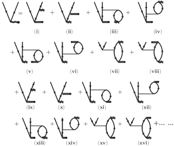
Figure 10: Goldstone diagrams representing last four terms of Eq. (87) representing the $u^{PV\pm}$ term that give rise to DCP contributions in the CPDF-RPA method. Diagrams from (ix) to (xvi) along with their exchanges are coming due to the implementation of the orthogonalization condition.

Like Eqs. (44) and (45), both Eqs. (64) and (65) are also solved iteratively to obtain the self-consistent solutions to account for core-polarization effects to all-orders. Using the above APV modified orbitals, $E1_{PV}$ can be evaluated as

$$E1_{PV}=\langle f|d|i^{PV}\rangle+\langle f^{PV}|d|i\rangle.$$ (66)

To make one-to-one comparison between contributions arising through the CPDF method and other many-body methods including lower-order terms of the RMBPT(3) method, we can present the CPDF expression for $E1_{PV}$ using the wave operators as

$$E1_{PV}=\langle\Phi_{f}|D\Omega^{i,CPDF}|\Phi_{i}\rangle+\langle\Phi_{f}|\Omega^{f,CPDF\dagger}D|\Phi_{i}\rangle,$$ (67)

where $\Omega^{v,CPDF}=\Omega_{0}^{CPDF}+\Omega_{v}^{CPDF}=\sum_{k=1}^{\infty}\left[\sum_{a,p}\Omega_{a,p}^{(k,1)}+\sum_{p}\Omega_{v,p}^{(k,1)}\right]$ with subscripts $0$ and $v$ stand for operators responsible for including core and valence correlations, and superscript $k$ denotes order of $V_{res}$. Amplitudes of these operators are given by

$$\Omega_{a,p}^{(k,1)} = \Omega_{a}^{p}+\sum_{b,q}\Big{(}\frac{[\langle pb|g|aq\rangle-\langle pb|g|qa\rangle]}{\epsilon_{a}-\epsilon_{p}}\Omega_{b,q}^{(k-1,1)}$$ (68)

$$+\Omega_{b,q}^{{(k-1,1)}^{\dagger}}\frac{[\langle pq|g|ab\rangle-\langle pq|g|ba\rangle]}{\epsilon_{a}-\epsilon_{p}}\Big{)}$$

and

$$\Omega_{v,p}^{(k,1)} = \Omega_{v}^{p}+\sum_{b,q}\Big{(}\frac{[\langle pb|g|vq\rangle-\langle pb|g|qv\rangle]}{\epsilon_{v}-\epsilon_{p}}\Omega_{b,q}^{(k-1,1)}$$ (69)

$$+\Omega_{b,q}^{{(k-1,1)}^{\dagger}}\frac{[\langle pq|g|vb\rangle-\langle pq|g|bv\rangle]}{\epsilon_{v}-\epsilon_{p}}\Big{)},$$

where the sums over $a,b$ and $p,q$ represent occupied and virtual operators respectively. To compute amplitude of the above operators, we set $\Omega_{a,p}^{(0,1)}\approx\Omega_{a}^{p}$ and $\Omega_{v,p}^{(0,1)}\approx\Omega_{v}^{p}$ in the beginning to initiate the iteration procedure from $k=1$. As can be followed here that only the effective singly excited configurations are contributing through the $\Omega^{v,CPDF}$ operators. Thus, it completely misses out pair-correlation contributions.

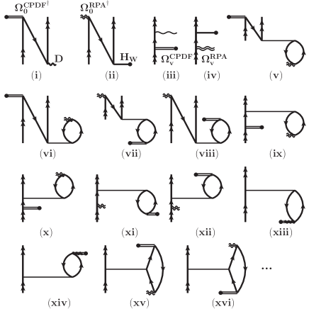
Figure 11: Goldstone diagrams contributing to the $E1_{PV}$ amplitude in the CPDF-RPA method. Comparing these diagrams with the diagrams of the RMBPT(3) method, can be understood by expanding the $\Omega_{0/v}^{CPDF}$, $\Omega_{0/v}^{RPA}$ and $\Omega^{CPDF\pm}$ operators, it can be followed that the CPDF-RPA method does not include contributions from pair-correlation effects and some of the DCP effects representing diagrams.

The Goldstone diagrams that contribute to the amplitudes of $\Omega_{0}^{CPDF}$ are shown in Fig. 4. Similarly, the Goldstone diagrams contributing to the amplitudes of $\Omega_{v}^{CPDF}$ are shown in Fig. 5. Using these operators, we show the final Goldstone diagrams that contribute to $E1_{PV}$ in Fig. 6. By analyzing these diagrams in terms of the Goldstone diagrams shown in Figs. 4 and 5, it is easy to follow how the core-polarization effects are included to all-orders through the CPDF method. Again, comparing those diagrams with the diagrams from the DHF and RMBPT(3) methods the relations among them can be easily understood. One can also realize here that number of Goldstone diagrams appear in the CPDF method are very less than the RMBPT(3) method. Thus, the computational efforts in the CPDF method are much smaller compared to the RMBPT(3) method though it is an all-order theory.

IV.4 RPA

From Eq. (66), it can be followed that the CPDF method includes correlation effects in the first-order wave functions through the $H_{W}$ operator only. Thus, it completely misses out correlation effects in the unperturbed state that can arise through the $D$ operator. It can also be noted that the CPDF method is formulated based on Eq. (15). Therefore proceeding with a similar manner based on Eq. (30), it can lead to capturing core-polarization effects through the $D$ operator and the RPA is formulated exactly on the same line.

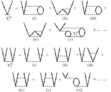
Figure 12: Goldstone diagrams demonstrating breakdown of the $T^{(0)}$ operators in terms of lower-order perturbative excitations.

To derive the RPA expression, we consider the net Hamiltonian $H_{int}^{\pm}=H+\lambda_{3}D\mp\omega$ to define the modified single particle DHF Hamiltonian $f_{i}^{\pm}=f_{i}+\lambda_{3}d\mp\omega$ and potential as

$$f_{i}^{\pm}|\tilde{i}^{\pm}\rangle=\tilde{\epsilon}_{i}^{\pm}|\tilde{i}^{\pm}\rangle$$ (70)

and

$$\tilde{u}_{i}^{\pm}=\sum_{b}^{N_{c}}\left[\langle\tilde{b}^{\pm}|g|\tilde{b}^{\pm}\rangle|\tilde{i}^{\pm}\rangle-\langle\tilde{b}^{\pm}|g|\tilde{i}^{\pm}\rangle|\tilde{b}^{\pm}\rangle\right],$$ (71)

respectively, where the superscript $\pm$ denotes solution for $H_{int}^{\pm}$ in place of $H$. Now expanding $|i^{\pm}\rangle=|i\rangle+\lambda_{3}|i^{\pm}\rangle+{\cal O}(\lambda_{3}^{2})$ and retaining terms that are linear in $\lambda_{3}$, we can get

$$(f_{i}-\epsilon_{i}\mp\omega)|i^{\pm}\rangle=-d|i\rangle-u_{i}^{\pm}|i\rangle,$$ (72)

where

$$u_{i}^{\pm}|i\rangle=\sum_{b}^{N_{c}}\left[\langle b|g|b\rangle|i^{\pm}\rangle-\langle b|g|i^{\pm}\rangle|b\rangle\right.$$

$$\left.+\langle b^{\mp}|g|b\rangle|i\rangle-\langle b^{\mp}|g|i\rangle|b\rangle\right].$$ (73)

Here also both Eqs. (72) and (73) are solved iteratively to obtain the self-consistent solutions to account for core-polarization effects to all-orders. Using the above $D$ operator modified orbitals, $E1_{PV}$ can be evaluated as

$$E1_{PV}=\langle\Phi_{f}|H_{W}\Omega^{i,+}|\Phi_{i}\rangle+\langle\Phi_{f}|\Omega^{f,-\dagger}H_{W}|\Phi_{i}\rangle,$$ (74)

where $\Omega^{v,\pm}=\Omega_{0}^{\pm}+\Omega_{v}^{\pm}=\sum_{k=1}^{\infty}\left[\sum_{a,p}\Omega_{a,p}^{\pm(k,1)}+\sum_{p}\Omega_{v,p}^{\pm(k,1)}\right]$ with subscripts $0$ and $v$ stand for operators responsible for including Core and Valence correlations, and superscript $k$ denotes order of $V_{res}$. Amplitudes of these operators are given by

$$\Omega_{a,p}^{\pm(k,1)} = \Omega_{a}^{p\pm}+\sum_{b,q}\Big{(}\frac{[\langle pb|g|aq\rangle-\langle pb|g|qa\rangle]}{\epsilon_{a}-\epsilon_{p}\pm\omega}\Omega_{b,q}^{\pm(k-1,1)}$$ (75)

$$+\Omega_{b,q}^{\mp{(k-1,1)}^{\dagger}}\frac{[\langle pq|g|ab\rangle-\langle pq|g|ba\rangle]}{\epsilon_{a}-\epsilon_{p}\pm\omega}\Big{)}$$

and

$$\Omega_{v,p}^{\pm(k,1)} = \Omega_{v}^{p\pm}+\sum_{b,q}\Big{(}\frac{[\langle pb|g|vq\rangle-\langle pb|g|qv\rangle]}{\epsilon_{v}-\epsilon_{p}\pm\omega}\Omega_{b,q}^{\pm(k-1,1)}$$ (76)

$$+\Omega_{b,q}^{{\mp(k-1,1)}^{\dagger}}\frac{[\langle pq|g|vb\rangle-\langle pq|g|bv\rangle]}{\epsilon_{v}-\epsilon_{p}\pm\omega}\Big{)},$$

where we assume $\Omega_{a,p}^{\pm(0,1)}\approx\Omega_{a}^{p\pm}$ and $\Omega_{v,p}^{\pm(0,1)}\approx\Omega_{v}^{p\pm}$ initially for the iteration procedure. We also intend to mention here is that in Eqs. (75) and (76) , $\omega$ value can be used from the experiment while in the ab initio framework it is taken from the DHF method. Following the explanation in the previous sub-section, it is obvious that the RPA wave operators will pick up core-polarization correlations through the $D$ operator to all-orders. Again based on the classification adopted in this work, the Goldstone diagrams contributing to the amplitude determining equation for Core operator are shown in Fig. 7, while the diagrams contributing to the amplitudes of the Valence operator are shown in Fig. 8.

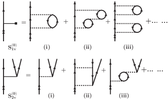
Figure 13: Goldstone diagrams demonstrating breakdown of the $S_{v}^{(0)}$ operators in terms of lower-order perturbative excitations.

Using the above operators, we show the final Goldstone diagrams that contribute to $E1_{PV}$ of RPA in Fig. 9. By analyzing these diagrams in terms of the Goldstone diagrams shown in Figs. 7 and 8, it can be followed how the core-polarization effects are included through $D$ to all-orders through the RPA. Again, comparing these diagrams with the diagrams from the DHF and RMBPT(3) methods the relations among both the methods can be understood. Though the number of Goldstone diagrams appear in the RPA and the CPDF method are same, but amplitudes in the CPDF method are expected to converge faster than the RPA owing to strong correlations arising through $D$ than $H_{W}$. It can be noticed here that the Core correlations (without DHF contributions) arising in the RPA are distinctly different than that appear via the CPDF method.

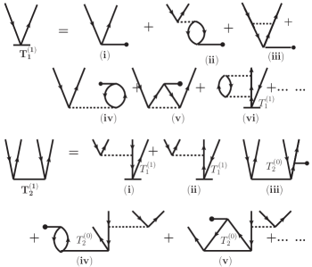
Figure 14: Goldstone diagrams demonstrating breakdown of the $T^{(1)}$ operators in terms of lower-order perturbative excitations.

IV.5 CPDF-RPA/TDHF method

As realized above, the CPDF method and the RPA include core-polarization effects only through the first-order perturbed wave functions but the unperturbed wave functions and energies in both the cases are used from the DHF method. In order to achieve core-polarization effects through both the states it is necessary to include the $H_{W}$ and $D$ operators in the perturbation. The simplest approach for doing so would be to add both the CPDF and RPA results and remove repeated appearance of the DHF value from one of the approaches. However, such an approach would omit correlations among both the $H_{W}$ and $D$ operators which may not be negligible.

Keeping in view of the above, we define the total Hamiltonian as

$$H_{t} = H+\lambda_{2}H_{W}+\lambda_{3}D$$ (77)

$$\equiv H_{int}+\lambda_{3}D.$$

Treating both the $H_{W}$ and $D$ operators perturbatively, the exact atomic wave function ($|\overline{\Psi}_{v}\rangle$) of $H_{t}$ can be expressed as

$$|\overline{\Psi}_{v}\rangle = |\Psi_{v}^{(0,0)}\rangle+\lambda_{2}|\Psi_{v}^{(1,0)}\rangle+\lambda_{3}|\tilde{\Psi}_{v}^{(0,1)}\rangle$$ (78)

$$+\lambda_{2}\lambda_{3}|\Psi_{v}^{(1,1)}\rangle+\cdots.$$

As denoted earlier, $|\Psi_{v}^{(m,n)}\rangle$ represents consideration of $m$ orders of $H_{w}$ and $n$ orders of $D$ in the atomic wave function $|\Psi_{v}\rangle$ of $H$. In the wave operator formalism, it is given by

$$\overline{\Omega}_{v}|\Phi_{v}\rangle = \Omega_{v}^{(0,0)}|\Phi_{v}\rangle+\lambda_{2}\Omega_{v}^{(1,0)}|\Phi_{v}\rangle+\lambda_{3}\tilde{\Omega}_{v}^{(0,1)}|\Phi_{v}\rangle$$ (79)

$$+\lambda_{2}\lambda_{3}\Omega_{v}^{(1,1)}|\Phi_{v}\rangle+\cdots,$$

where superscripts denote the same meaning as above. It can be noted that each $\Omega_{v}^{(m,n)}$ component will have parts carrying Core and Valence correlations separately.

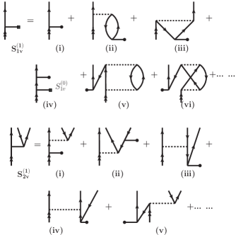
Figure 15: Goldstone diagrams demonstrating breakdown of the $S_{v}^{(1)}$ operators in terms of lower-order perturbative excitations.

In this case, we can determine the $E1_{PV}$ amplitude as the transition amplitude of $O\equiv\lambda_{2}H_{w}+\lambda_{3}D$ between the initial perturbed state to the final unperturbed state or between the initial unperturbed state to the final perturbed state (see Eqs. (31) and (32)). i.e.

$$E1_{PV} = \langle\Psi_{f}^{(0,0)}|\Psi_{i}^{(1,1)}\rangle+\langle\Psi_{f}^{(0,0)}|D|\Psi_{i}^{(1,0)}\rangle$$ (80)

$$+\langle\Psi_{f}^{(0,0)}|H_{W}|\tilde{\Psi}_{i}^{(0,1)}\rangle$$

$$= \langle\Phi_{f}|\Omega_{f}^{(0,0)\dagger}\Omega_{i}^{(1,1)}|\Phi_{i}\rangle+\langle\Phi_{f}|\Omega_{f}^{(0,0)\dagger}D\Omega_{i}^{(1,0)}|\Phi_{i}\rangle$$

$$+ \langle\Phi_{f}|\Omega_{f}^{(0,0)\dagger}H_{W}\tilde{\Omega}_{i}^{(0,1)}|\Phi_{i}\rangle$$

or

$$E1_{PV} = \langle\Psi_{f}^{(1,1)}|\Psi_{i}^{(0,0)}\rangle+\langle\Psi_{f}^{(1,0)}|D|\Psi_{i}^{(0,0)}\rangle$$ (81)

$$+\langle\tilde{\Psi}_{f}^{(0,1)}|H_{W}|\Psi_{i}^{(0,0)}\rangle$$

$$= \langle\Phi_{f}|\Omega_{f}^{(1,1)\dagger}\Omega_{i}^{(0,0)}|\Phi_{i}\rangle+\langle\Phi_{f}|\Omega_{f}^{(1,0)\dagger}D\Omega_{i}^{(0,0)}|\Phi_{i}\rangle$$

$$+ \langle\Phi_{f}|\tilde{\Omega}_{f}^{(0,1)\dagger}H_{W}\Omega_{i}^{(0,0)}|\Phi_{i}\rangle,$$

keeping terms that are of the order of $\lambda_{2}\lambda_{3}$. Note that both $H_{W}$ and $D$ operators are treated on an equal footing in this approach. Thus, definitions of both Core and Valence contributions to $E1_{PV}$ will be identical for both Eqs. (80) and (81). Also, it would be prudent to use both the expressions in an approximated method to verify numerical uncertainty to the final result. However, if $\omega^{ex}$ (some earlier studies have done it through the scaling procedure) is used then the results from both these equations may not agree to each other due to inconsistencies in the treatment of the intermediate states through these equations.

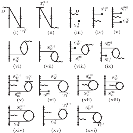
Figure 16: A few important $E1_{PV}$ evaluating diagrams in the RCCSD method. Diagrams shown as $DT^{(1)}$ and its complex conjugate (c.c.)) term are the dominant Core contributing effects that include all the core-polarization effects of the CPDF method, pair-correlation effects of the RMBPT(3) method and their correlations. Similarly, diagrams shown as $DS_{1i}^{(1)}$ and $S_{1f}^{(1)\dagger}D$ contain Valence contributing core-polarization effects of the CPDF method, pair-correlation effects from the RMBPT(3) method and their correlations. $DS_{2i}^{(1)}$ and $S_{2f}^{(1)\dagger}D$ representing diagrams contain Core contributions from the RPA and DCP contributions from the CPDF-RPA method as well as that are absent in this method but appears in the RMBPT(3) method. Non-linear RCCSD terms incorporate higher-order correlation effects of the above terms and account correlations among core-polarization, pair-correlation and their intercombinations.

The modified single particle Hamiltonian for the corresponding Hamiltonian $H_{t}=H_{int}+\lambda_{3}D$ in the CPDF-RPA method can be written as $f_{i}^{PV\pm}=f_{i}^{PV}+\lambda_{3}d\mp\omega$. It follows

$$f_{i}^{PV\pm}|\overline{i}\rangle=\overline{\epsilon}_{i}|\overline{i}\rangle$$ (82)

and

$$\overline{u}_{i}=\sum_{b}^{N_{c}}\left[\langle\overline{b}|g|\overline{b}\rangle|\overline{i}\rangle-\langle\overline{b}|g|\overline{i}\rangle|\overline{b}\rangle\right],$$ (83)

where the bar symbol denotes solution for $H_{t}$. By expanding, we get $|\overline{i}\rangle=|i^{PV}\rangle+\lambda_{3}|i^{PV\pm}\rangle+{\cal O}(\lambda_{3}^{2})$. It gives

$$(f_{i}^{PV}-\epsilon_{i}^{PV}\mp\omega)|i^{PV\pm}\rangle=-d|i^{PV}\rangle-u_{i}^{PV(1)}|i^{PV}\rangle,$$ (84)

where

$$u_{i}^{PV(1)}|i^{PV}\rangle=\sum_{b}^{N_{c}}\left[\langle b^{PV}|g|b^{PV}\rangle|i^{PV\pm}\rangle\right.$$

$$\left.-\langle b^{PV}|g|i^{PV\pm}\rangle|b^{PV}\rangle\right.$$

$$\left.+\langle b^{PV}|g|b^{PV}\rangle|i^{PV\pm}\rangle\right.$$

$$\left.-\langle b^{PV}|g|i^{PV\pm}\rangle|b^{PV}\rangle\right].$$ (85)

Further expanding Eqs. (84) and (85), and retaining terms of the order of $\lambda_{2}\lambda_{3}$ we get

$$(f_{i}-\epsilon_{i}\mp\omega)|i^{PV\pm}\rangle = -d|i^{PV}\rangle-u_{i}^{\pm}|i^{PV}\rangle-h_{w}|i^{\pm}\rangle$$ (86)

$$-u_{i}^{PV}|i^{\pm}\rangle-u_{i}^{PV\pm}|i\rangle,$$

where

$$u_{i}^{PV\pm}|i\rangle=\sum_{b}^{N_{c}}\left[\langle b^{\mp}|g|b^{PV}\rangle|i\rangle\right.$$

$$\left.-\langle b^{\mp}|g|i\rangle|b^{PV}\rangle\right.$$

$$\left.+\langle b^{PV}|g|b^{\pm}\rangle|i\rangle\right.$$

$$\left.-\langle b^{PV}|g|i\rangle|b^{\pm}\rangle\right.$$

$$\left.+\langle b|g|b^{PV\pm}\rangle|i\rangle\right.$$

$$\left.-\langle b|g|i\rangle|b^{PV\pm}\rangle\right.$$

$$\left.+\langle b^{PV\mp}|g|b\rangle|i\rangle\right.$$

$$\left.-\langle b^{PV\mp}|g|i\rangle|b\rangle\right].$$ (87)

Table 1: $E1_{PV}$ values, in units $10^{-11}i(-Q_{w}/Nn)|e|a_{0}$, of the $6s~{}^{2}S_{1/2}-7s~{}^{2}S_{1/2}$ and $6s~{}^{2}S_{1/2}-5d~{}^{2}D_{3/2}$ transitions in ¹³³Cs from DC Hamiltonian reported by various works. Methods shown as ‘Sum-over’ and ‘Mixed’ are obtained using sum-over-states approach and mixed many-body methods respectively. Results shown in bold fonts are claimed to be within 0.5% accuracy.

Method	This work	Others	This work	Others
$6s~{}^{2}S_{1/2}-7s~{}^{2}S_{1/2}$			$6s~{}^{2}S_{1/2}-5d~{}^{2}D_{3/2}$
DHF	$0.7375$	$0.736$ [11]	$-2.3933$
RMBPT(3)w	$1.0902$		$-2.4639$
CPDF	$0.9226$	$0.924$ [11]	$-2.7989$
RPA	$0.7094$	$0.707$ [11]	$-2.2362$
CPDF-RPA∗	$0.8876$	$0.8914$ [25]	$-3.1665$	$-3.70$ [37]
		$0.8923^{\dagger}$ [25]
CPDF-RPA	$0.8844$	$0.886$ [11]	$-3.0281$	$-3.80$ [26]
		$0.907$ [26]
RCCSD	$0.8964$	$0.8961$ [29]	$-3.5641$	$-3.210$[38]
RCCSDT		0.8967 [29]
Sum-over		$0.9053$ [24]		$-3.76$ [13]
		0.8998† [24]
Mixed-states		$0.8967$ [25]	$-3.62$ [13]
		0.8938† [25]
		0.9083‡ [25]
†Note: Scaled value.
‡Scaled value $+$ borrowed contribution from Ref. [24].

Table 2: Reduced E1 (in a.u.) and $H_{W}$ (in units of $10^{-11}i(-Q_{w}/Nn)|e|a_{0}$) matrix elements from the RCCSD method, and the excitation energies (in cm^-1) of the low-lying states of ¹³³Cs that are used to estimate the ‘Main’ contribution of $E1_{PV}$ for the $6S-7S$ transition. E1 matrix elements and energies are compared with the available most precise experimental values.

Transition	E1 amplitude		Excitation Energy		$H_{W}$ amplitude
	This work	Experiment	This work	Experiment [45]
$6P_{1/2}$-$6S$	$4.5487$	$4.5097(74)$ [41]	$-11243.93$	$-11178.27$	$-1.2541$
$7P_{1/2}$-$6S$	$0.3006$	$0.2825(20)$ [42]	$-21838.93$	$-21765.35$	$-0.7135$
$8P_{1/2}$-$6S$	$0.0914$		$-25787.48$	$-25708.83$	$-0.4808$
$9P_{1/2}$-$6S$	$-0.0388$		$-27735.96$	$-27637.00$	$0.3471$
$6P_{1/2}$-$7S$	$-4.2500$	$4.233(22)$[43]	$7352.53$	$7357.26$	$0.6067$
$7P_{1/2}$-$7S$	$10.2967$	$10.308(15)$[44]	$-3242.47$	$-3229.82$	$0.3445$
$8P_{1/2}$-$7S$	$0.9492$		$-7191.02$	$-7173.31$	$0.2320$
$9P_{1/2}$-$7S$	$-0.3867$		$-9139.50$	$-9101.47$	$-0.1674$

It can be further noted that in the CPDF method the perturbed core DHF orbital ($|a^{PV}\rangle$) is orthogonal to the unperturbed core orbital ($|a\rangle$) and the same is also true in the RPA. i.e. $\langle a|a^{PV}\rangle=0$ and $\langle a|a^{\pm}\rangle=0$. However, $\langle a|a^{PV\pm}\rangle\neq 0$ in the CPDF-RPA method. This necessitates to use the orthogonalized core orbitals ($|a^{o\pm}\rangle$) by imposing the condition

$$|a^{o\pm}\rangle = |a^{PV\pm}\rangle-\sum_{b}|b\rangle\langle b|a^{PV\pm}\rangle.$$ (88)

In Fig. 10, we show the Goldstone diagrams contributing to the determination of the $|a^{PV\pm}\rangle$ and also the extra diagrams that are subtracted to obtain $|a^{o\pm}\rangle$. It can be understood below that it is not required to obtain the modified orbitals for the virtual orbitals in the CPDF-RPA method to estimate the $E1_{PV}$ amplitude, so we do not show Goldstone diagrams contributing to the amplitudes of valence operator here.

Using the following expressions in the formula given by Eq. (80), we can write

$$E1_{PV} = \langle f|d+u_{i}^{+}|i^{PV}\rangle+\langle f|h_{w}+u_{i}^{PV}|i^{+}\rangle$$ (89)

$$+\langle f|u_{i}^{PV+}|i\rangle.$$

Similarly, using the formula given by Eq. (81) we can get

$$E1_{PV} = \langle f^{PV}|d+u_{i}^{+}|i\rangle+\langle f^{-}|h_{w}+u_{i}^{PV}|i\rangle$$ (90)

$$+\langle f|u_{f}^{PV-}|i\rangle$$

$$= \langle f^{PV}|d+u_{i}^{+}|i\rangle+\langle f^{-}|h_{w}+u_{i}^{PV}|i\rangle$$

$$+\langle f|u_{i}^{PV+}|i\rangle.$$

In the wave operator form, Eq. (89) can be given by

$$E1_{PV} = \langle\Phi_{f}|D\Omega^{i,CPDF}|\Phi_{i}\rangle+\langle\Phi_{f}|H_{w}\Omega^{i,+}|\Phi_{i}\rangle$$ (91)

$$+\langle\Phi_{f}|\Omega^{CPDF+}|\Phi_{i}\rangle.$$

From (90), we can write

$$E1_{PV} = \langle\Phi_{f}|\Omega^{f,CPDF\dagger}D|\Phi_{i}\rangle+\langle\Phi_{f}|\Omega^{-\dagger}H_{w}|\Phi_{i}\rangle$$ (92)

$$+\langle\Phi_{f}|\Omega^{f,CPDF-}|\Phi_{i}\rangle$$

$$= \langle\Phi_{f}|\Omega^{f,CPDF\dagger}D|\Phi_{i}\rangle+\langle\Phi_{f}|\Omega^{f,-\dagger}H_{w}|\Phi_{i}\rangle$$

$$+\langle\Phi_{f}|\Omega^{CPDF+}|\Phi_{i}\rangle.$$

In the above expressions, we define

$$\Omega^{CPDF+}=\sum_{i,j}(\langle f|u_{i}^{+}|i^{PV}\rangle+\langle f|u_{i}^{PV}|i^{+}\rangle$$

$$+\langle f|u_{i}^{PV+}|i\rangle)a_{j}^{\dagger}a_{i}$$ (93)

and

$$\Omega^{CPDF-}=\sum_{i,j}(\langle f^{PV}|u_{f}^{-}|i\rangle+\langle f^{-}|u_{f}^{PV}|i\rangle$$

$$+\langle f|u_{f}^{PV-}|i\rangle)a_{j}^{\dagger}a_{i}$$ (94)

It is also worth noting that some of the works in the literature do not consider contribution from $\langle f|u_{i}^{PV+}|i\rangle$ in the CPDF-RPA method, and their contributions are separately quoted as ‘DCP’ effects. In Fig. 11, we show the diagrams that are contributing to $E1_{PV}$ in the CPDF-RPA method icluding the DCP effect. Now comparing diagrams from Fig. 11 and the diagrams from the RMBPT(3) method shown in Fig. 2, it can be shown that some of the Core and Valence correlation diagrams of the RMBPT method are appearing as the Core diagrams of the CPDF-RPA method (so also for Valence contributions). This, therefore, clearly demonstrates that the definitions of Core and Valence correlation contributions to $E1_{PV}$ are not unique and their classifications differ based on the approach adopted in a many-body method. Among the approximated methods where various physical effects or correlation effects through both the $H_{W}$ and $D$ operators are not included on an equal footing, it may not be possible to make an one-to-one comparative analysis among contributions arising through the Core and Valence correlations. In such a scenario, it is suggestive to compare only the final results from different methods.

The advantages of using the CPDF-RPA method are that this method includes core-polarization effects to all-orders, treats both the $H_{W}$ and $D$ operators on an equal footing (which means the results would remain invariant in what-so-ever order either $H_{W}$ or $D$ is included in $H_{t}$ along with $H$), and gives DCP effects that are not present in the CPDF method or RPA. However, it still misses out many non-core-polarization effects including pair-correlation contributions and correlations among core-polarization, and pair-correlation effects in the determination of $E1_{PV}$. Again, orthogonalization of perturbed occupied orbitals is incorporated by hand while the approach does not take care of them in a natural manner. We would like to mention that some of the earlier calculations using the CPDF-RPA method neglected contributions from the DCP effects (see Ref. [26]). Results from such as an approximation are denoted as CPDF-RPA* method. In fact, omission of some of the DCP contributions in this method is just due to a similar reason. Moreover, the CPDF, RPA and CPDF-RPA methods cannot be derived using Bloch’s prescription though we have expressed them using wave operators just to make one-to-one connection of these methods with the RMBPT method. Thus, these methods are simply the extension of the DHF method and cannot take into account the effects that may have been neglected in generating the single particle orbitals. For example, the effects of $V^{N}$, $V^{N-1}$, $V^{N-2}$ etc. potentials used in the determination of wave functions through the Bloch equation are taken care through an effective Hamiltonian like $H_{eff}=P_{v}V_{res}\Omega_{v}^{(0)}P_{v}$ that appears in solving amplitude of $\Omega_{v}^{(0)}$. However, the wave operator amplitude solving equations in the CPDF, RPA and CPDF-RPA methods remain to be the same. Thus, the valence electron interaction neglected in the construction of DHF potential (inactive valence orbital) is not amended through the above methods like in the RMBPT method. All these shortcomings of the CPDF-RPA method will be adequately addressed by the RCC method.

Table 3: Estimated ‘Main’ contributions to the $E1_{PV}$ values, in units $10^{-11}i(-Q_{w}/Nn)|e|a_{0}$, of the $6s~{}^{2}S_{1/2}-7s~{}^{2}S_{1/2}$ transition in ¹³³Cs using matrix elements involving $np~{}^{2}P_{1/2}$ intermediate states in the sum-over-states approach. Four cases are being considered: (a) ab initio result in which calculated values from Table 2 are used; (b) replacing calculated E1 matrix elements by their experimental values; (c) retaining calculated E1 matrix elements and using experimental energies; and (d) using experimental values for both E1 matrix elements and energies.

Approach	$\langle 7S|D|6S^{PNC}\rangle$	$\langle 7S^{PNC}|D|6S\rangle$	Total
(a)	$-0.4461$	$1.3171$	$0.8710$
(b)	$-0.4373$	$1.3121$	$0.8748$
(c)	$-0.4522$	$1.3156$	$0.8634$
(d)	$-0.4434$	$1.3106$	$0.8672$

IV.6 RCC method

The RCC method both in the non-relativistic and its counter relativistic forms have been extensively considered these days to include electron correlation effects in the determination of properties of different types of many-body systems accurately such as nuclear, atomic, molecular and solid state systems. This is the reason for which these days it is commonly referred to as the gold standard of many-body theory. Compared to the CPDF, RPA and CPDF-RPA methods, implementation and computational efforts in the RCC method are extensively complex and expensive. It can account correlations through both the $H_{W}$ and $D$ operators to all-orders, as well take care other shortcomings of the CPDF-RPA method. All CPDF-RPA effects along with other effects like pair-correlations, inter-correlations among core-polarization and pair-correlation effects, corrections due to choice of $V^{N-1}$ DHF potential approximation etc. are sub-summed within our RCC method. This theory was already implemented and results using the method were already reported for Cs [21, 23], Ba⁺ [21], Yb⁺ [39] and Ra⁺ [40]. Here, we consider this theory in the singles and doubles approximation (RCCSD method) only to demonstrate how it captures correlations of previously mentioned methods including appearance of orthogonalization of perturbed core orbitals in a natural fashion, all-order pair-correlations, additional DCP effects and normalization of wave functions etc. compared to a mixed many-body method. Since all these effects are present within the RCC theory and the wave functions are obtained through iterative scheme, all of these effects are inter-correlated. Incorporation of additional effects from the Breit and QED interactions can also be treated in the similar fashion, if their corresponding interaction potential terms are added in the atomic Hamiltonian. Going beyond the RCCSD method approximation in the RCC theory such as the RCCSDT method, means it can capture even higher-order non core-polarization effects and further inter-correlations among core-polarization and pair-correlation effects that are beyond the reach of the mixed many-body methods employed earlier to estimate the $E1_{PV}$ amplitudes. As shown in Ref. [29] though the energies, E1 matrix elements and magnetic dipole hyperfine structure constants from both the RCCSD and RCCSDT methods were quite significant, the difference in the $E1_{PV}$ values from both these two methods was rather small. This suggests that consideration of the RCCSD method would be sufficient enough to address the earlier mentioned concerns.

In the RCC theory framework, the exact wave function of an atomic state can be given by

$$|\Psi_{v}\rangle=e^{S}|\Phi_{v}\rangle,$$ (95)

where $S$ is an excitation operator carrying out excitations of electrons out of core orbitals from the DHF wave function $|\Phi_{v}\rangle$ to generate the excited state configurations due to $V_{res}$. In other words, these excitation configurations can be thought of as contributions taken from each order of corrections to the wave function from the RMBPT method to construct an all-order form. We can further define

$$S=T+S_{v},$$ (96)

in order to distinguish excitations of electrons among the core orbitals, denoted by $T$, and excitations of electrons from valence orbital or valence orbital along with core orbitals, denoted by $S_{v}$ in the $V^{N-1}$ framework of constructing the DHF wave function $|\Phi_{v}\rangle=a_{v}^{\dagger}|\Phi_{0}\rangle$. Accordingly we can write

$$|\Psi_{v}\rangle = e^{T+S_{v}}|\Phi_{v}\rangle$$ (97)

$$= e^{T}\left\{1+S_{v}\right\}|\Phi_{v}\rangle.$$

Here $e^{S_{v}}=1+S_{v}$ is the exact form for the atomic states having one valence orbital $v$. In the RCCSD method, the excitation operators are denoted as

$$T=T_{1}+T_{2}$$ (98)

and

$$S_{v}=S_{1v}+S_{2v},$$ (99)

where subscripts 1 and 2 stand for the singles and doubles excitations respectively.

Table 4: Core and Valence correlation contributions to the $E1_{PV}$ values, in units $10^{-11}i(-Q_{w}/Nn)|e|a_{0}$, for the $6s~{}^{2}S_{1/2}-7s~{}^{2}S_{1/2}$ and $6s~{}^{2}S_{1/2}-5d~{}^{2}D_{3/2}$ transitions in ¹³³Cs from the RMBPT(3)^w and RMBPT(3)^d approaches. Results (a) considering $H_{eff}$ effect due to $V^{N-1}$ potential and (b) using DHF orbital energies are shown for comparison.

Approach	RMBPT(3)w		RMBPT(3)d
	Core	Valence	Core	Valence
		$6s~{}^{2}S_{1/2}-7s~{}^{2}S_{1/2}$
(a)	$-0.00205$	$1.09220$	$-0.00003$	$1.24290$
(b)	$-0.00206$	$0.43938$	$-0.00031$	$0.43763$
		$6s~{}^{2}S_{1/2}-5d~{}^{2}D_{3/2}$
(a)	$-0.16391$	$-2.30000$	$-0.12208$	$-2.55427$
(b)	$-0.18267$	$-3.97004$	$-0.12513$	$-4.02758$

In the wave operator form given by Eqs. (7) and (8), it corresponds to

$$\Omega_{0}=e^{T}$$ (100)

and

$$\Omega_{v}=e^{T}S_{v}.$$ (101)

Following the Bloch’s equations given by Eqs. (9) and (10) in general form, amplitudes of the $T$ and $S_{v}$ excitation operators are obtained by

$$\langle\Phi_{0}^{*}|(He^{T})_{l}|\Phi_{0}\rangle=0$$ (102)

and

$$\langle\Phi_{v}^{*}|[(He^{T})_{l}-E_{v}]S_{v}|\Phi_{v}\rangle=-\langle\Phi_{v}^{*}|(He^{T})_{l}|\Phi_{v}\rangle,$$ (103)

where subscript $l$ denotes for the linked terms, bra states with superscript $*$ means excited states with respect to the respective DHF ket states appear in the equations. In the ab initio procedure, the energy of the $|\Psi_{v}\rangle$ is determined by calculating expectation value of the effective Hamiltonian i.e.

$$E_{v} = \langle\Phi_{v}|H_{eff}|\Phi_{v}\rangle$$ (104)

$$= \langle\Phi_{v}|P_{v}(He^{T})_{l}\left\{1+S_{v}\right\}P_{v}|\Phi_{v}\rangle,$$

with respect to $|\Phi_{v}\rangle$. As can be noticed $E_{v}$ is a function of $S_{v}$ and $S_{v}$ itself depends on $E_{v}$. Thus, the non-linear Eqs. (103) and (104) are solved iteratively to obtain amplitudes of $S_{v}$. As pointed out earlier, appearance of $E_{v}$ in the determination of $S_{v}$ amplitudes is a consequence of using orbitals from $V^{N-1}$ potential. It is also possible to obtain amplitudes of the RCC operators by substituting experimental energy in the semi-empirical approach. Also, one can scale the $S_{v}$ amplitudes by multiplying by a suitable parameter $\lambda$ to obtain the calculated $E_{v}$ value matching with the experimental energy in the similar spirit of the scaling procedures adopted in Refs. [24] and [25].

Table 5: Ab initio contributions to Core and Valence parts of the $E1_{PV}$ values, in units $10^{-11}i(-Q_{w}/Nn)|e|a_{0}$, for the $6s~{}^{2}S_{1/2}-7s~{}^{2}S_{1/2}$ and $6s~{}^{2}S_{1/2}-5d~{}^{2}D_{3/2}$ transitions in ¹³³Cs from different methods considered in this work using the DC Hamiltonian. Available results from previous calculations are also given for comparison.

Method	This work		Others
	Core	Valence	Core	Valence
$6s~{}^{2}S_{1/2}-7s~{}^{2}S_{1/2}$
DHF	$-0.00173$	$0.73923$	$-0.00174$[30]
RMBPT(3)w	$-0.00205$	$1.09220$
RMBPT(3)d	$-0.00003$	$1.24290$
CPDF	$-0.00199$	$0.92454$	$-0.00201$ [30]
RPA	$0.00028$	$0.70912$
CPDF-RPA∗	$0.00169$	$0.88591$	$0.00170$ [30]
CPDF-RPA	$0.00169$	$0.88267$
RCCSD	$-0.00197$	$0.89840$	$-0.0019$ [29]	$0.8980$ [29]
$6s~{}^{2}S_{1/2}-5d~{}^{2}D_{3/2}$
DHF	$-0.11684$	$-2.27646$
RMBPT(3)w	$-0.16391$	$-2.3000$
RMBPT(3)d	$-0.12208$	$-2.55427$
CPDF	$-0.19122$	$-2.60768$
RPA	$-0.12037$	$-2.11585$
CPDF-RPA∗	$-0.20786$	$-2.95860$
CPDF-RPA	$-0.20786$	$-2.82021$
RCCSD	$-0.14745$	$-3.41667$

To evaluate $E1_{PV}$, we need to express the RCC operators in terms of both the unperturbed and first-order perturbed operators. As explained in Sec. III, we have three different options to obtain the $E1_{PV}$ amplitude in the RCC theory framework. First, by adopting the approach similar to the CPDF method, in which $H_{W}$ is considered as external perturbation and matrix element of $D$ can be determined. Second, considering $D$ as the external perturbative operator as in the RPA. Third and the most effective approach would be along the line of the CPDF-RPA method, in which, both the $H_{W}$ and $D$ operators can be treated as external perturbations. The implementation of the third approach would be more challenging and computationally very expensive as it will demand to store amplitudes of four different types of perturbed RCC operators instead of storing only one type of perturbed amplitudes in the first case and two types in the second case. Among the first two approaches, computational efforts are almost similar but implementation-wise considering $H_{W}$ as perturbation will be more natural and is easier to deal with its angular momentum couplings owing to its scalar form. Moreover, amplitudes of the perturbed operators due to $H_{W}$ will converge faster than when $D$ is treated as perturbation. Again, it is possible to use experimental energies in the first approach to obtain semi-empirical results in case it is required while it is a problem in the second case owing to the fact that is already discussed earlier. From this view, we adopt the first approach to estimate the $E1_{PV}$ value.

We expand the $T$ and $S_{v}$ operators by treating $H_{W}$ as the perturbation to separate out the solutions for the unperturbed and the first-order wave functions by expressing

$$T=T^{(0)}+\lambda_{2}T^{(1)}$$ (105)

and

$$S_{v}=S_{v}^{(0)}+\lambda_{2}S_{v}^{(1)},$$ (106)

where the superscript meanings are same as specified earlier. This yields

$$|\Psi_{v}^{(0)}\rangle = (\Omega_{0}^{(0)}+\Omega_{v}^{(0)})|\Phi_{v}\rangle$$ (107)

and

$$|\Psi_{v}^{(1)}\rangle=(\Omega_{0}^{(1)}+\Omega_{v}^{(1)})|\Phi_{v}\rangle$$ (108)

with the definitions $\Omega_{0}^{(0)}=e^{T^{(0)}}$, $\Omega_{0}^{(1)}=e^{T^{(0)}}T^{(1)}$, $\Omega_{v}^{(0)}=e^{T^{(0)}}S_{v}^{(0)}$ and $\Omega_{v}^{(1)}=e^{T^{(0)}}\left\{T^{(1)}S_{v}^{(0)}+S_{v}^{(1)}\right\}$. The unperturbed operator amplitudes are obtained by solving the usual RCC theory equations as mentioned above. The first-order perturbed RCC operator amplitudes are determined as

$$\langle\Phi_{0}^{*}|(He^{T^{(0)}})_{l}T^{(1)}|\Phi_{0}\rangle=-\langle\Phi_{0}^{*}|(H_{W}e^{T^{(0)}})_{l}|\Phi_{0}\rangle$$ (109)

and

$$\langle\Phi_{v}^{*}|[(He^{T^{(0)}})_{l}-E_{v}^{(0)}]S_{v}^{(1)}|\Phi_{v}\rangle=-\langle\Phi_{v}^{*}|[(H_{W}e^{T^{(0)}})_{l}$$

$$+(He^{T^{(0)}})_{l}T^{(1)}]\{1+S_{v}^{(0)}\}|\Phi_{v}\rangle\ \ \ \$$ (110)

As can be seen, the exact calculated energy also enters into the amplitude determining equation of $S_{v}^{(1)}$ because of the $V^{N-1}$ potential. This is one of the advantages of the RCC method over the CPDF-RPA method. In Figs. 12,13, 14, 15 we show some of the important Goldstone diagrams contributing to the $T_{2}^{(0)}$, $T_{1}^{(0)}$, $S_{1v}^{(0)}$, $T_{2}^{(1)}$,$T_{1}^{(1)}$,$S_{2v}^{(0)}$, $S_{1v}^{(1)}$ and $S_{2v}^{(1)}$ amplitudes. These diagrams can be compared with the CPDF-RPA wave operator amplitude determining diagrams in order to understand how they are embedded within the RCC operators irrespective of the fact that denominators in the RCC method will contain the exact energy of the state instead of the DHF energy in the CPDF-RPA method.

The $E1_{PV}$ expression between the states $|\Psi_{i}\rangle$ and $|\Psi_{f}\rangle$ in the RCC theory is given by

$$E1_{PV}=\frac{\langle\Phi_{f}|\{S_{f}^{(1)\dagger}+(S_{f}^{(0)\dagger}+1)T^{(1)\dagger}\}\bar{D}\{1+S_{i}^{(0)}\}|\Phi_{i}\rangle}{\langle\Phi_{f}|\{S_{f}^{(0)\dagger}+1\}\bar{N}\{1+S_{i}^{(0)}\}|\Phi_{i}\rangle}$$

$$+\frac{\langle\Phi_{f}|\{S_{f}^{(0)\dagger}+1\}\bar{D}\{T^{(1)}(1+S_{i}^{(0)})+S_{i}^{(1)}\}|\Phi_{i}\rangle}{\langle\Phi_{f}|\{S_{f}^{(0)\dagger}+1\}\bar{N}\{1+S_{i}^{(0)}\}|\Phi_{i}\rangle},\ \ \$$ (111)

where $\bar{D}=e^{T^{(0)+}}De^{T^{(0)}}$ and $\bar{N}=e^{T^{(0)+}}e^{T^{(0)}}$. Unlike the CPDF, RPA and CPDF-RPA methods, normalization factors appear explicitly in the RCC expression. Using the wave operator notations, one can easily identify which RCC terms contribute to the Core and Valence correlations in the evaluation of $E1_{PV}$. It means basically, any term is connected either with the $S_{n=i,f}{{}^{(0/1)}}$ operators or with their conjugate operators will be a part of the Valence correlation otherwise they will be a part of the Core correlation. It can be further clarified that the definitions of Core and Valence correlation contributions to $E1_{PV}$ in our RCC theory are in the line of the RMBPT(3)^w and CPDF methods, and different than the RPA and CPDF-RPA methods. In Fig. 16 we show a few important contributing Goldstone diagrams from the RCC method to Core and Valence correlations. Also, for better understanding, the Goldstone diagrams of the RCCSD operators are further demonstrated as the sum of lower-order Goldstone diagrams of the RMBPT(3) method. From these relations, it can be followed that the RCC method includes correlation effects from core-polarization, pair-correlation, and DCP to all orders. It is also obvious from the above diagrams that orthogonalization to core orbitals and extra DCP contributions are also appearing in a natural manner in our RCC theory. Moreover, correlations among all these effects are implicitly present due to the fact that singles and doubles excitation amplitude equations are coupled through many non-linear terms in the RCC theory.

Table 6: Comparison of contributions from the initial and final perturbed states to $E1_{PV}$ of the $6s~{}^{2}S_{1/2}-7s~{}^{2}S_{1/2}$ transition of ¹³³Cs, in units $10^{-11}i(-Q_{w}/Nn)|e|a_{0}$, at different levels of approximation between the present work and that are reported in Refs. [11, 30].

Method	$\langle{7S}^{PNC}|D|6S\rangle$		$\langle 7S|D|6S^{PNC}\rangle$
	Ours	Ref. [11]	Ours	Ref. [11]
	Total contribution
DHF	$1.01168$	$1.010$	$-0.27418$	$-0.274$
CPDF	$1.26664$	$1.267$	$-0.34409$	$-0.344$
RPA	$1.02557$	$1.023$	$-0.31617$	$-0.316$
CPDF-RPA*	$1.27910$	$1.279$	$-0.39150$	$-0.391$
	Ours	Ref. [30]	Ours	Ref. [30]
	Core contribution
DHF	$-0.02638$	$-0.02645$	$0.02465$	$0.02472$
CPDF	$-0.04298$	$-0.04319$	$0.04099$	$0.04119$
RPA	$-0.03536$		$0.03564$
CPDF-RPA*	$-0.05794$	$-0.05822$	$0.05963$	$0.05992$
Valence contribution
DHF	$1.03806$		$-0.29883$
CPDF	$1.30962$		$-0.38508$
RPA	$1.06094$		$0.70912$
CPDF-RPA*	$1.33704$		$-0.45113$

V Results & Discussions

We present the calculated values of $E1_{PV}$ of the $6S-7S$ and $6S-5D_{3/2}$ transitions in ¹³³Cs from the DHF, RMBPT(3), CPDF, RPA, CPDF-RPA and RCCSD methods. As mentioned in Introduction, the main intention of carrying out this study is to demonstrate similarities and differences among various contributions to $E1_{PV}$ through the above methods. This would be useful in addressing the issue of the sign for the Core correlation contributions to the $E1_{PV}$ value of the $6S-7S$ transition in ¹³³Cs that are reported differently by various groups [24, 25, 29]. Moreover, this exercise would be useful in understanding the missing contributions in a method compared to others that are under consideration here so that accuracy of the earlier reported results in an atomic system, including Cs, obtained using a particular method can be further improved. We have allowed correlations from all the occupied orbitals and allowed excitations of electrons from a given set of virtual orbitals in all the considered many-body methods to make comparative analysis of results from them. In order to show that we have taken a sufficiently large set basis functions, we validate our calculations by comparing our $E1_{PV}$ values from the DHF, CPDF, RPA and CPDF-RPA methods with the earlier reported values by Mårtensson [11]. The reason for presenting the $E1_{PV}$ value of the $6S-5D_{3/2}$ transition in ¹³³Cs is to answer to a comment by Roberts and Ginges in Ref. [30], where they argue about the agreement of the sign of Core contribution to the $E1_{PV}$ value of a $S-D$ transition reported earlier using the RCCSD method [40] while observing a sign difference for the $6S-7S$ transition in ¹³³Cs.

In Table 1, we present the $E1_{PV}$ values of the $6S-7S$ and $6S-5D_{3/2}$ transitions in ¹³³Cs using the DC Hamiltonian from a number of methods including the DHF method in order to understand the importance of correlation effects in their determination and to demonstrate that choice of a method matters a lot for their rigourous inclusion. The values shown in bold fonts in this table are claimed to be accurate within 0.5% by the earlier works. A careful look into these results reveal that some of them differ by 1% from each other, which suggests there could be issues with the estimation of accuracy in these calculations that needs to be investigated. Results from sum-over-states approach, given as ‘Sum-over’ in the table, uses scaled E1 matrix elements and energies from the CCSDvT method to estimate the Main contribution of $E1_{PV}$ for the $6S-7S$ transition while the X-factor is obtained using a blend of many-body methods [24]. In Ref. [25], the same ‘Main’ contribution is utilized but Core and Tail contributions to the X-factor are estimated using the CPDF-RPA* method (denoted as only RPA in the original paper). Pair-correlation effects to these estimations were estimated using the BO-correlation method. Result from these RPA$+$BO methods is given under ‘Mixed-states’ in the above table. Thus large discrepancy seen in both the results from the above table come from the X-factors estimated in Refs [24, 25]. If the total X-factors had agreed between two works but individual contributions would have differed, then the difference in the results could have been attributed to distribution of contributions under the Core and Valence correlations in the considered approaches in both the works. From the significant differences seen between the X-factors from the Mixed-states approach and our RCCSD method in both the $6S-7S$ and $6S-5D_{3/2}$ transitions, it does not support such distributions.

To understand the reasons for significant discrepancies seen in the X-factors from various works, we first analyze the Main contribution to the $6S-7S$ transition by using the calculated properties from our RCCSD method in the sum-over-states approach. We used the E1 matrix elements and energies from our calculations as well as from experiments to show the differences. In Table 2, we present the $H_{W}$ matrix elements, E1 matrix elements and energies obtained using the DC Hamiltonian in the RCCSD method. The calculated E1 matrix elements and energies are also compared with the experimental values [41, 42, 43, 44, 45] in the same table. Using these values we estimate the Main contributions to $E1_{PV}$ of the $6S-7S$ transition and they are given in Table 3. Results (a) from ab initio calculations, (b) using experimental E1 values with calculated energies, (c) calculated E1 values with experimental energies and (d) using experimental values for both the E1 matrix elements and energies are given separately. This analysis shows that result from (b) is larger than (a), but results from (c) and (d) are lower than (a). It means that accuracy of energies in a given method affect the results more than E1 matrix elements. Later we demonstrate explicitly that it introduces error to $E1_{PV}$ estimation when we use experimental energy only of the initial or final state through the first-principle calculations. Differences between the ab initio and semi-empirical calculations can be minimised by including contributions from the triples, quadruples etc. higher-level excitations of the RCC method. In Ref. [29], Sahoo et al have demonstrated difference between the ab initio calculations of $E1_{PV}$ of the $6S-7S$ transition using the RCCSD and RCCSDT methods is very small. They further showed that Core contributions are almost same in both the methods, and the agreement of the $E1_{PV}$ values from both the methods was the result of opposite trends of correlation effects in the evaluation of the $H_{W}$ matrix elements than the E1 matrix elements and energies. A similar trend was anticipated from the Tail contribution. Subtracting the ab initio value of Main from the final RCCSD result, we find the X-factor to $E1_{PV}$ of the $6S-7S$ transition as 0.0254, against 0.0175 and 0.0256 of Refs. [24] and [25] respectively in units of $10^{-11}i(-Q_{w}/Nn)|e|a_{0}$. It means that there is a large difference between the X-factor of Ref. [24] and our work, whereas these values almost agree between Ref. [25] and the present work. Since there is a sign difference between the Core contribution from Ref. [25] and the RCCSD value of Ref. [29], the above analysis suggests that the sign difference is solely due to different definitions used for the Core contribution in both the works.

In order to explain how definition of Core contribution changes depending upon the choice of an approach to estimate $E1_{PV}$, we present the Core and Valence contributions separately to the $6S-7S$ and $6S-5D_{3/2}$ transitions from both the RMBPT(3)^w and RMBPT(3)^d approaches in Table 4. Just for the sake of demonstrating how appearance of $H_{eff}$ in the wave function determining equation due to choice of $V^{N-1}$ modify the result, we present RMBPT(3) results considering effect of $H_{eff}$ (given results as (a) in the above table) and replacing it with DHF energy as the case of the CPDF-RPA method (corresponding results are given under (b) in the above table). As can be seen, the Core and Valence contributions from both the RMBPT(3)^w and RMBPT(3)^d approaches are coming out differently whereas the final results from both the methods are almost close to each other. It can also be realized that changes in the results for both the transitions are enormous when $H_{eff}$ is considered in the wave function solving equation than otherwise.

Table 7: Contributions to Core and Valence parts from different terms to $E1_{PV}$ of the $6s~{}^{2}S_{1/2}-7s~{}^{2}S_{1/2}$ and $6s~{}^{2}S_{1/2}-5d~{}^{2}D_{3/2}$ transitions in ¹³³Cs, in units $10^{-11}i(-Q_{w}/Nn)|e|a_{0}$ from Eqs. (89) and (90) of the CPDF-RPA method, which are quoted under ‘Expression a’ and ‘Expression b’ respectively. Results are given using the calculated $\omega$ value, $\omega^{ex}$ and $\omega^{ex}$ with the experimental energies of the initial and final states (denoted by $E_{i,f}^{expt}$).

Contribution	Expression a			Expression b
	$6s~{}^{2}S_{1/2}-7s~{}^{2}S_{1/2}$
	$\langle 7s|h_{w}|6s^{+}\rangle$	$\langle 7s|u_{6s}^{PV}|6s^{+}\rangle$	Total	$\langle 7s^{PV}|d|6s\rangle$	$\langle 7s^{PV}|u_{6s}^{+}|6s\rangle$	Total
Core ($\omega$)	$-0.0357$	$-0.02257$	$-0.05794$	$-0.04299$	$-0.01495$	$-0.05794$
Valence ($\omega$)	$1.06094$	$0.27610$	$1.33704$	$1.30962$	$0.02742$	$1.33704$
Core ($\omega^{ex}$)	$-0.03464$	$-0.02211$	$-0.05675$	$-0.04299$	$-0.01458$	$-0.05757$
Valence ($\omega^{ex}$)	$-0.19464$	$-0.04598$	$-0.24062$	$1.30962$	$0.02743$	$1.33705$
Core ($E_{i,f}^{expt}$)	$-0.03546$	$-0.02283$	$-0.05829$	$-0.04331$	$-0.01498$	$-0.05829$
Valence ($E_{i,f}^{expt}$)	$1.21721$	$0.31956$	$1.53677$	$1.53384$	$0.00293$	$1.53677$
	$\langle 7s|d|6s^{PV}\rangle$	$\langle 7s|u_{6s}^{+}|6s^{PV}\rangle$	Total	$\langle 7s^{-}|h_{w}|6s\rangle$	$\langle 7s^{-}|u_{6s}^{PV}|6s\rangle$	Total
Core ($\omega$)	$0.04099$	$0.01864$	$0.05963$	$0.03564$	$0.023399$	$0.05963$
Valence ($\omega$)	$-0.38508$	$-0.06605$	$-0.45113$	$-0.35181$	$-0.09932$	$-0.45113$
Core ($\omega^{ex}$)	$0.04099$	$0.01915$	$0.06014$	$0.03651$	$0.02458$	$0.06109$
Valence ($\omega^{ex}$)	$-0.38508$	$-0.06644$	$-0.45152$	$-0.17081$	$-0.05022$	$-0.22103$
Core ($E_{i,f}^{expt}$)	$0.04210$	$0.01999$	$0.06209$	$0.03686$	$0.02523$	$0.06209$
Valence ($E_{i,f}^{expt}$)	$-0.12128$	$-0.05800$	$-0.17928$	$-0.13743$	$-0.04185$	$-0.17928$
	$6s~{}^{2}S_{1/2}-5d~{}^{2}D_{3/2}$
	$\langle 5d_{3/2}|h_{w}|6s^{+}\rangle$	$\langle 5d_{3/2}|u_{6s}^{PV}|6s^{+}\rangle$	Total	$\langle 5d_{3/2}^{PV}|d|6s\rangle$	$\langle 5d_{3/2}^{PV}|u_{6s}^{+}|6s\rangle$	Total
Core ($\omega$)	$0.0$	$-0.00616$	$-0.00616$	$-0.00451$	$-0.00165$	$-0.00616$
Valence ($\omega$)	$0.0$	$-0.27386$	$-0.27386$	$-0.27878$	$0.00492$	$-0.27386$
Core ($\omega^{ex}$)	$0.0$	$-0.00612$	$-0.0612$	$-0.00451$	$-0.00164$	$-0.00615$
Valence ($\omega^{ex}$)	$0.0$	$-0.23287$	$-0.23287$	$-0.27878$	$0.00493$	$-0.27385$
Core ($E_{i,f}^{expt}$)	$0.0$	$-0.00628$	$-0.00628$	$-0.00459$	$-0.001087$	$-0.00628$
Valence ($E_{i,f}^{expt}$)	$0.0$	$-0.83936$	$-0.83936$	$-0.87962$	$0.04028$	$-0.83936$
	$\langle 5d_{3/2}|d|6s^{PV}\rangle$	$\langle 5d_{3/2}|u_{6s}^{+}|6s^{PV}\rangle$	Total	$\langle 5d_{3/2}^{-}|h_{w}|6s\rangle$	$\langle 5d_{3/2}^{-}|u_{6s}^{PV}|6s\rangle$	Total
Core ($\omega$)	$-0.19574$	$-0.00596$	$-0.20170$	$-0.12037$	$-0.08133$	$-0.20170$
Valence ($\omega$)	$-2.88646$	$0.20172$	$-2.68474$	$-2.11585$	$-0.56889$	$-2.68474$
Core ($\omega^{ex}$)	$-0.19574$	$-0.00636$	$-0.20210$	$-0.12109$	$-0.08182$	$-0.20291$
Valence ($\omega^{ex}$)	$-2.88646$	$0.20201$	$-2.68445$	$-1.94829$	$-0.52407$	$-2.47236$
Core ($E_{i,f}^{expt}$)	$-0.20110$	$-0.00744$	$-0.20854$	$-0.12363$	$-0.08491$	$-0.20854$
Valence($E_{i,f}^{expt}$)	$-2.02306$	$0.16022$	$-1.86284$	$-1.46451$	$-0.39833$	$-1.86284$

To further figure out about the mismatch in the X-factors from various works, we present the Core and Valence contributions to the $E1_{PV}$ values separately for both the $6S-7S$ and $6S-5D_{3/2}$ transitions arising through the first-principle calculations in Table 5. As can be seen from the table, signs of Core contributions to $E1_{PV}$ of both the transitions from the DHF method and many-body methods at a given level of approximation employed by different groups match each other. This indicates that there is no issue with the implementation of these theories in our code. To support results from our methods further, we also compare Core and Valence contributions to the $6S-7S$ transition in Table 6 from the initial and final perturbed states through the DHF, CPDF, RPA and CPDF-RPA* methods with the values reported in a Comment by Roberts and Ginges [30], and Mårtensson [11]. We find reasonably good agreement between our results with the earlier estimations. As it has been explained in the previous section, definitions of Core correlation effects arising through the CPDF, RPA and CPDF-RPA methods all differ. Thus, the exact reason for which sign of Core contribution to $E1_{PV}$ of the $6S-7S$ transition in ¹³³Cs differ between Ref. [24] and Ref. [25] is not clear to us as the exact method(s) employed in Ref. [24] for its estimation is not mentioned explicitly. Only from the sign of the Core contribution quoted in Ref. [24] and by comparing it with the signs of Core contributions from the RMBPT(3)^w, CPDF and RCCSD methods of the present work and from the RCCSD and RCCSDT methods of Ref. [29], we can assume that Ref. [24] estimates Core contribution by considering $H_{W}$ as perturbation. In such a case, the Tail contributions to $E1_{PV}$ for the $6S-7S$ transition in ¹³³Cs from Refs. [24] and [29] as well as from the RCCSD result of the present work should almost agree each other on the basis of the argument that the net X-factor value should agree irrespective of the fact that whether $H_{W}$ or $D$ is treated as perturbation. Large differences between the X-factors from Refs. [24], [25] and this work, which report as 0.0175, 0.0256 and 0.0254 in units of $10^{-11}i(-Q_{w}/Nn)|e|a_{0}$, suggests that the former work underestimates the Tail contribution. It should be noted that the Tail contributions are estimated without using sum-over-states approach in all the works, so the difference in these values are mainly due to different levels of approximation made in the many-body methods employed for their estimations.

Table 8: First-principle calculated $E1_{PV}$ values (in $-i(Q_{W}/Nn)ea_{0}\times 10^{-11}$) of the $6s~{}^{2}S_{1/2}-7s~{}^{2}S_{1/2}$ and $6s~{}^{2}S_{1/2}-5d~{}^{2}D_{3/2}$ transitions in ¹³³Cs from different terms of the RCCSD method. Both ab initio and scaled values are given for comparison. We have used two different types of scaling: (a) only scaling amplitudes of the the unperturbed $S_{v}^{(0)}$ operators and (b) scaling amplitudes of both the $S_{v}^{(0)}$ and $S_{v}^{(1)}$ operators. Here, contributions under ‘Norm’ represents the difference between the contributions after and before normalizing the RCCSD wave functions. ‘Others’ denote contributions from those RCCSD terms that are not shown explicitly in this table.

RCC term	$6s^{2}S_{1/2}-7s~{}^{2}S_{1/2}$			$6s~{}^{2}S_{1/2}-5d~{}^{2}D_{3/2}$
	Ab initio	Scaled-a	Scaled-b	Ab initio	Scaled-a	Scaled-b
	Core contribution
$\overline{D}T_{1}^{(1)}$	$-0.04161$	$-0.04161$	$-0.04161$	$-0.00062$	$-0.00062$	$-0.00062$
$T_{1}^{(1)\dagger}\overline{D}$	$0.03964$	$0.03964$	$0.03964$	$-0.17132$	$-0.17132$	$-0.17132$
Others	$-0.00005$	$-0.00005$	$-0.00005$	$0.01757$	$0.01757$	$0.01757$
Norm	$0.00005$	$0.00005$	$0.00005$	$0.00692$	$0.00670$	$0.00670$
	Valence contribution
$\overline{D}S_{1i}^{(1)}$	$-0.19363$	$-0.19363$	$-0.19688$	$-2.96310$	$-2.96310$	$-2.97589$
$S_{1f}^{(1)\dagger}\overline{D}$	$1.80382$	$1.80382$	$1.80263$	$-0.89993$	$-0.89993$	$-1.30760$
$S_{1f}^{(0)\dagger}\overline{D}S_{1i}^{(1)}$	$-0.23184$	$-0.23187$	$-0.23297$	$-0.06863$	$-0.06548$	$-0.06487$
$S_{1f}^{(1)\dagger}\overline{D}S_{1i}^{(0)}$	$-0.41826$	$-0.41895$	$-0.41942$	$0.10487$	$0.10502$	$0.14626$
$\overline{D}S_{2i}^{(1)}$	$-0.00039$	$-0.00039$	$-0.00039$	$0.00107$	$0.00107$	$0.00108$
$S_{2f}^{(1)\dagger}\overline{D}$	$0.00033$	$0.00033$	$0.00033$	$-0.00023$	$-0.00023$	$-0.00023$
Others	$-0.04040$	$-0.04222$	$-0.04025$	$0.24888$	$0.24806$	$0.27704$
Norm	$-0.02122$	$-0.01942$	$-0.02110$	$0.16040$	$0.15505$	$0.15309$
Total	$0.89643$	$0.89570$	$0.88998$	$-3.56412$	$-3.56721$	$-3.91879$

Now, we wish to address the reason why Roberts and Ginges were able to get same sign for the Core contribution to $E1_{PV}$ of the $7S-6D_{3/2}$ transition in Ra⁺ using their RPA$+$BO method with that are reported using the RCC method in Ref. [40]. Since correlation trends to $E1_{PV}$ of the $nS-(n-1)D_{3/2}$ transitions are almost similar in Cs and Ra⁺, with the ground state principal quantum number $n$ of the respective system, we can understand the above point by analysing the Core contributions to $E1_{PV}$ of the $6S-5D_{3/2}$ transition from different methods and comparing their trends with the $6S-7S$ transition of ¹³³Cs. By looking at these contributions from Table 5, it can be easily followed that there is one-order magnitude difference between the Core contribution in the $6S-7S$ transition from the RMBPT(3)^w and RMBPT(3)^d methods while there is a sign change between these results from the CPDF method and the RPA. However, the difference between the Core contributions from the RMBPT(3)^w and RMBPT(3)^d methods in the $6S-5D_{3/2}$ transition are small, and there is no sign difference between the CPDF and RPA results. These trends can be explained as follows. In the $6S-7S$ transition, wave functions of both the associated states have large overlap over the nucleus while in the $6S-5D_{3/2}$ transition only the wave function of the ground state has large overlap with the nucleus. As a result, strong core-polarization effects contribute through both the states in the former case. Also, contribution from individual diagram of the CPDF-RPA method is almost comparable in the $6S-7S$ transition, while a selective diagrams contribute predominantly in the $6S-5D_{3/2}$ transition. Since core-polarization effects arising through the $D$ operator are stronger and have opposite signs than that arise through $H_{W}$, the net Core contributions in the $S-S$ and $S-D$ transitions behave very differently in the CDHF method and RPA, and the same propagates to the CPDF-RPA*/CPDF-RPA method. Since Core and Valence contributions are basically redistributed in the CPDF-RPA* and RCCSD methods, difference between the final values between Refs. [25] and [29] as well as from the present work are coming out to be very small in the $6S-7S$ transition, while it is slightly noticeable in the $6S-5D_{3/2}$ transition (refer to Table 1 for the comparison of results from the Mixed-states and RCCSD methods) .

The DCP contributions from our calculations can be estimated by taking the differences in the results from the CPDF-RPA* and CPDF-RPA methods. This difference for the $6S-7S$ transition from our work is compared with the corresponding values from Refs. [11] and [26]. From this comparison, we find that our result agrees better with Roberts than Mårtensson. However, our final CPDF-RPA result agrees well with Ref. [11] than Ref. [26]. We also intend to mention that the CPDF-RPA* results in Refs. [25] and [30] are also scaled by using $\omega^{ex}=0.0844$ a.u.. In the previous section, we have justified theoretically why such an approach would lead to errors in the determination of the $E1_{PV}$ values. To demonstrate it numerically, we have given results for both the $6S-7S$ and $6S-5D_{3/2}$ transitions from the CPDF-RPA method using Eqs. (89) and (90) in Table 7. We have given these values using $\omega$, $\omega^{ex}$ and then also using $\omega^{ex}$ and experimental energies (denoted by $E_{i,f}^{expt}$) of the $6S$, $7S$ and $5D_{3/2}$ states. From the comparison of the results, we observe a very a interesting trend. When both $\omega$ and energies of the atomic states are considered either from theory or experiment, results from both Eqs. (89) and (90) match each other, otherwise large discrepancies are seen. In the RMBPT, RPA or CPDF-RPA method, it is possible to use $\omega^{ex}$ and experimental energies of the initial and final states simultaneously in the $E1_{PV}$ evaluating expressions. However, one can either use $\omega^{ex}$ or $\omega^{ex}$ with experimental energy of only the valence state (whose perturbed state wave function is evaluated) in the complicated methods like the RCC method. Energies of the double, triple excited configurations appear in the denominator of the RCC theory, their experimental energies cannot be used in the wave function determining equations. By corroborating this fact with the above finding, it can be said that scaling the wave function by using experimental energy of the valence state alone may not always give accurate result, rather it may introduce additional error to the calculation. As explained in the previous section, this fact can be theoretically understood using Eq. (41). Nevertheless, it can be found from Table 7 that our result with $\omega^{ex}$ value from the CPDF-RPA* method does not match with the corresponding results from Refs. [25, 30] for the $6S-7S$ transition. We are unable to understand the reason for this though results with theoretical $\omega$ value from both the works agree quite well.

As mentioned in Sec. IV, three different approaches can be adopted in any many-body theory framework for evaluation of the $E1_{PV}$ amplitudes. The same applies to the RCC theory as well. However, we adopt the approach of evaluating the matrix element of the $D$ operator after considering $H_{W}$ as the external perturbation. Though this approach is in the line with the CPDF method, it is effectively takes care of electron correlation effects through both the $H_{W}$ and $D$ operators as in the CPDF-RPA method. In fact, it goes much beyond the CPDF-RPA method to include the electronic correlation effects which will be evident from the follow-up discussions. It means that it is possible to deduce all the CPDF-RPA contributions from the RCC theory, which is even true at the level of the RCCSD method approximation. In this sense that the RCCSDT method employed by Sahoo et al. [29] to estimate the $E1_{PV}$ amplitude of the $6S-7S$ transition in ¹³³Cs includes the RPA contributions that are mentioned in Refs. [25, 30]. However, some of these contributions are not a part of the Core contribution rather they come through the Valence contribution in our RCCSD method owing to the fact that the $D$ operator is not treated as an external perturbation here to determine the perturbed atomic wave functions. This point can be comprehend from the comparison between the RMBPT(3)^w and RMBPT(3)^d results, which are propagated to all-orders in the RCC theory. To define Core contributions in the line of CPDF-RPA method, the RCC theory of $E1_{PV}$ can be derived either treating the $H_{W}$ and $D$ operators simultaneously as external perturbation or perturbing wave functions by considering one of these operators as external perturbation and evaluating matrix element of the other operator in the normal-order RCC theory framework similar to that is discussed in Ref. [46]. Among the choices of considering one of them as the external perturbation, it is advisable to use $H_{W}$ as perturbation in which evaluation of perturbed wave function in an iterative scheme can converge faster. In fact, this should also be the natural choice from the APV theory point of view and is being adopted here. In order to understand the Core and Valence contributions to the $E1_{PV}$ amplitudes from our RCCSD method, we can take the help of the diagrams from the RMBPT(3)^w method. Since wave operator amplitude determining equations for both the methods follow the same Bloch’s prescription, all physical effects appear in the RMBPT(3)^w method are present to all-orders in the RCCSD method. It means that the core-polarization effects and additional lower-order DCP contributions that arise in the RMBPT(3)^w method are present to all-orders in the RCCSD method. In the CPDF-RPA method, core-polarization effects are appearing through the single excitations while the DCP effects are implicitly present through the double excitations in the RCCSD method. Similarly, the pair-correlation effects of the RMBPT(3)^w method are present to all-orders through the single excitations in the RCCSD method. Since both single and double excitation amplitude solving equations are coupled in the RCCSD method, correlations among all these physical effects are taken into account in this method. Again through the non-linear terms from the exponential form of the RCCSD method, higher-order correlation effects, neither a part of core-polarization or pair-correlation types, are also included in the RCCSD method. It is not possible to include these effects systematically using a blend of many-body methods.

In Table 8, we present the $E1_{PV}$ values of the $6S-7S$ and $6S-5D_{3/2}$ transitions in ¹³³Cs from individual RCCSD terms to fathom the discussions of the previous paragraph quantitatively. By using definitions of the $T$ and $S_{v}$ RCC excitation operators, we categorized the results into Core and Valence correlation contributions. By subtracting the Core contributions of the DHF method from the contributions of the $\bar{D}T_{1}^{(1)}$ and its complex conjugate (c.c.) term, the net Core correlation contributions to $E1_{PV}$ in the RCCSD method can be inferred. Similarly by subtracting the Valence contributions of the DHF method from the $\bar{D}S_{1i}^{(1)}+S_{1f}^{(1)\dagger}\bar{D}$ terms and adding contributions from other Valence correlation contributing terms, we can get the net Valence correlation contributions to $E1_{PV}$ in the RCCSD method. The Core correlations arising through $\bar{D}T_{1}^{(1)}$ and c.c. terms contain correlation contributions from both the singly and doubly excited configurations. By analysing the RMBPT(3)^w diagrams contributing to the $T_{1}^{(1)}$ amplitude determining equation shown in Fig. 14, it can be understood that the $\bar{D}T_{1}^{(1)}$ and c.c. terms contain the Core contributions of the CPDF method, pair-correlation contributions of the RMBPT(3) method to all-orders and many more. By analyzing diagrams from $\bar{D}T_{1}^{(1)}$ and their breakdown in terms of the RMBPT(3)^w method carefully, it can be evident that this term does not include Core contributions arising through the RPA and some of the contributions that arise through the CPDF-RPA method. Similarly, all the Valence correlation contributions from the CPDF method, RPA and CPDF-RPA* method are included through the $\bar{D}S_{1i}^{(1)}+S_{1f}^{(1)\dagger}\bar{D}$ terms in the RCCSD method. In addition, they also include many contributions that can appear through the BO-correlation technique and beyond. However, a lot more correlation contributions to $E1_{PV}$ arise through other RCCSD terms among which correlation contributions arising through $\bar{D}S_{2i}^{(1)}$, $\bar{D}T_{1/2}^{(1)}S_{1/2i}^{(0)}$, $T_{1/2}^{(1)\dagger}\bar{D}S_{1/2i}^{(0)}$, such terms but replacing $S_{1/2i}^{(0/1)}$ operators with $S_{1/2f}^{(0/1)\dagger}$, $S_{1/2f}^{(0)\dagger}\bar{D}S_{1/2i}^{(1)}$, $S_{1/2f}^{(1)\dagger}\bar{D}S_{1/2i}^{(1)}$ etc. terms in the RCCSD method. Obviously, these contributions are not present in the CPDF-RPA* method and many of them cannot be considered as a part of the BO-correlation method. Moreover, corrections to the entire correlation contributions including that appear through the CPDF-RPA method due to normalization of the wave functions (given as ‘Norm’) are quoted separately in the above table and they are found to be non-negligible. The most prominent DCP contributions are absorbed through the $\bar{D}S_{2i}^{(1)}+S_{2f}^{(1)\dagger}\bar{D}$ terms in the RCCSD method. Along with some of Core contributions from the CPDF-RPA method (like the ones appears in the RPA) are also included through these terms in the RCCSD method. In addition, non-linear terms $\bar{D}T_{1/2}^{(1)}S_{2i}^{(0)}$, $T_{2}^{(1)\dagger}\bar{D}S_{1i}^{(0)}$, $S_{2f}^{(0)\dagger}\bar{D}S_{2i}^{(1)}$ etc. including their c.c. terms posses a lot more Valence correlation contributions that are beyond the scope of considering by the combined CPDF-RPA and BO-correlation methods.

In Table 8, contributions to $E1_{PV}$ of the $6S-7S$ and $6S-5D_{3/2}$ transitions from the RCCSD terms using the scaled $S_{v}^{(0)}$ and $S_{v}^{(1)}$ amplitudes are also given. To show how the results vary with scaling both the unperturbed and perturbed wave functions independently, we present results after (a) scaling only the amplitudes of the $S_{v}^{(0)}$ operators and (b) then by scaling amplitudes of both the $S_{v}^{(0)}$ and $S_{v}{(1)}$ operators. Significant differences from both the scaled results are noticed. As mentioned before, it would not be correct to scale the $T^{(0/1)}$ amplitudes as orbitals used for their determination see $V^{N}$ potential against the amplitude determining equations for the $S_{v}^{(0/1)}$ operators, where orbitals see $V^{N-1}$ potential. Thus, substituting $\omega^{ex}$ value in the estimation of Core contribution may not be theoretically proper. Again, we can only substitute energy of the valence state from outside in the wave function solving equations, whereas energies of the intermediate states have to be generated implicitly in the RCC theory. It means that evaluating the $E1_{PV}$ amplitudes through the scaling procedure using the RCC method may introduce numerical errors to the calculations. Nonetheless, comparison of the semi-empirical results obtained by using experimental energies with the ab initio values of $E1_{PV}$ for both the $6S-7S$ and $6S-5D_{3/2}$ transitions shows that there are significant differences among them. These differences can be minimised by including higher-level excitations in the RCC theory. However, these higher-level excitations will not only improve the energy values but they will also change the matrix elements of the $H_{W}$ and $D$ operators. As shown by Sahoo et al. [29, 47] inclusion of the triple excitations in the RCC theory, modify the energies and the matrix elements of the $H_{W}$ and $D$ operators in such a way that the $E1_{PV}$ values from the RCCSD and RCCSDT methods almost remain to be same. From this argument, we cannot argue that the scaled $E1_{PV}$ values are more accurate than the ab initio values in the RCCSD method approximation.

VI Summary

By employing a number of relativistic many-body methods at different levels of approximation such as finite-order perturbation theory, coupled-perturbed Dirac-Fock method, random phase approximation, combined coupled-perturbed Dirac-Fock and random phase approximation method, and relativistic coupled-cluster theory, we investigated various roles of core and valence correlation effects in the calculations of the parity violating electric dipole amplitudes of the $6S\rightarrow 7S$ and $6S\rightarrow 5D_{3/2}$ transitions in ¹³³Cs. From this analysis, we were able to address a long standing issue of getting opposite signs to the core correlation contribution to the parity violating electric dipole amplitude of the aforementioned $6S\rightarrow 7S$ transition using the combined coupled-perturbed Dirac-Fock and random phase approximation methods. We also analysed results from the sum-over-states approach and first-principle calculations using the relativistic coupled-cluster method with singles and doubles approximation to figure out the missing contributions in the former approach. Inclusion of these missing contributions through the combined coupled-perturbed Dirac-Fock, random phase approximation and Brückener-orbital correlation methods is compared with the first-principle calculations using the coupled-cluster method. This comparison shows that the first-principle approach using the relativistic coupled-cluster theory incorporates electron correlation effects due to the Dirac-Coulomb Hamiltonian more rigorously than the other methods mentioned above in the evaluation of parity violating electric dipole amplitudes in the ¹³³Cs atom.

References

- [1] E. D. Commins, Quantum Mechanics An Experimentalists Approach, Cambridge University Press, New York (2003).
- [2] J. Erler and P. Langacker, Phys. Rev. Lett. 105, 031801 (2010).
- [3] W. J. Marciano and J. L. Rosner, Phys. Rev. Lett. 65, 2963 (1990); 68, 898 (1992).
- [4] M. -A. Bouchiat and C. Bouchiat, Phys. Lett. B 48, 111 (1974); J. Phys. (France) 35, 899 (1974).
- [5] P. Fayet, Phys. Lett. B 96, 83 (1980).
- [6] C. S. Wood, S. C. Bennet, D. Cho, B. P. Masterson, J. L. Roberts, C. E. Tanner and C. E. Wieman, Science 275, 1759 (1997).
- [7] J. Choi and D. S. Elliott, Phys. Rev. A 93, 023432 (2016).
- [8] A. Kastberg, T. Aoki, B. K. Sahoo, Y. Sakemi and B. P. Das, Phys. Rev. A 100, 050101(R) (2019).
- [9] V. A. Dzuba, V. V. Flambaum, P. G. Silvestrov and O. P. Sushkov, Phys. Lett. A 103, 265 (1984).
- [10] V. A. Dzuba, V. V. Flambaum, P. G. Silvestrov and O. P. Sushkov, J. Phys. B: Atom. Mol. Phys. 18, 597 (1985).
- [11] A. -M. Mårtensson-Pendrill, J. Phys. 46, 11 (1985).
- [12] S. A. Blundell, J. Sapirstein and W. R. Johnson, Phys. Rev. D 45, 5 (1992).
- [13] V. A. Dzuba, V. V. Flambaum and J. S. M. Ginges, Phys. Rev. D 63, 062101 (2001).
- [14] V. A. Dzuba, V. V. Flambaum and O. P. Sushkov, Phys. Lett. A 141, 147 (1989).
- [15] A. I. Milstein, O. P. Sushkov and I. S. Terekhov, Phys. Rev. Lett. 89, 283003 (2002).
- [16] B. A. Brown, A. Derevianko and V. V. Flambaum, Phys. Rev. C 79, 035501 (2009).
- [17] A. Derevianko, Phys. Rev. Lett. 85, 1618 (2000); Phys. Rev. A 65, 012106 (2001).
- [18] M. G. Kozlov, S. G. Porsev and I. I. Tupitsyn, Phys. Rev. Lett. 86, 3260 (2001).
- [19] V. M. Shabaev, K. Pachucki, I. I. Tupitsyn and V. A. Yerokhin, Phys. Rev. Lett. 94, 213002 (2005).
- [20] V. A. Dzuba, V. V. Flambaum and J. S. M. Ginges, Phys. Rev. D 66, 076013 (2002).
- [21] B. P. Das, B. K. Sahoo, G. Gopakumar, and R. K. Chaudhuri, J. Mol. Str. 768, 141 (2006).
- [22] B. K. Sahoo, Ph.D. thesis, Mangalore University, Karnataka, India, 2006, http://prints.iiap.res.in/handle/2248/680.
- [23] B. K. Sahoo, J. Phys. B 43, 085005 (2010).
- [24] S. G. Porsev, K. Beloy and A. Derevianko, Phys. Rev. D 82, 036008 (2010).
- [25] V. A. Dzuba, J. C. Berengut, V. V. Flambaum and B. Roberts, Phys. Rev. Lett. 109, 203003 (2012).
- [26] B. M. Roberts, V. A. Dzuba and V. V. Flambaum, Phys. Rev. A 88, 042507 (2013).
- [27] M. S. Safronova, D. Budker, D. DeMille, D. F. J. Kimball, A. Derevianko and C. W. Clark, Rev. Mod. Phys. 90, 025008 (2018).
- [28] C. Wieman and A. Derevianko, arXiv:1904.00281 (Unpublished).
- [29] B. K. Sahoo, B. P. Das and H. Spiesberger, Phys. Rev. D 103, L111303 (2021).
- [30] B. M. Roberts and J. S. M. Ginges, Phys. Rev. D 105, 018301 (2022).
- [31] H. B. Tran Tan, D. Xiao and A. Derevianko, Phys. Rev. A 105, 022803 (2022).
- [32] B. K. Sahoo, B. P. Das and H. Spiesberger, Phys. Rev. D 105, 018302 (2022).
- [33] R. N. Cahn and G. L. Kane, Phys. Lett. B 71, 348 (1977).
- [34] W. J. Marciano and A. I. Sanda, Phys. Rev. D 17, 3055 (1978).
- [35] E. D. Commins, Phys. Scr. T46, 92 (1993).
- [36] I. Lindgren and J. Morrison, Atomic Many-Body Theory, Springer-Verlag Berlin Heidelberg (1986).
- [37] B. M. Roberts, V. A. Dzuba and V. V. Flambaum, Phys. Rev. A 88, 012510 (2013).
- [38] A. Kastberg, B. K. Sahoo, T. Aoki, Y. Sakemi and B. P. Das, Symmetry 12, 974 (2020).
- [39] B. K. Sahoo, B. P. Das, Phys. Rev. A 84, 010502(R) (2011).
- [40] L. W. Wansbeek, B. K. Sahoo, R. G. E. Timmermans, K. Jungmann, B. P. Das and D. Mukherjee, Phys. Rev. A 78, 050501(R)(2008).
- [41] L. Young, W. T. Hill III, S. J. Sibener, S. D. Price, C. E. Tanner, C. E. Wieman and S. R. Leone, Phys. Rev. A 50, 2174 (1994).
- [42] A. A. Vasilyev, I. M. Savukov, M. S. Safronova and H. G. Berry, Phys. Rev. A 66, 020101 (2002).
- [43] M.-A. Bouchiat, J. Guena, and L. Pottier, J. Phys. (Paris), Lett. 45, 523 (1984).
- [44] S. C. Bennett, J. L. Roberts and C. E. Wieman, Phys. Rev. A 59, R16 (1999).
- [45] A. Kramida, Yu. Ralchenko, J. Reader and NIST ASD Team, NIST Atomic Spectra Database (ver. 5.6.1) (National Institute of Standards and Technology, Gaithersburg, MD, 2018).
- [46] B. K. Sahoo and B. P. Das, Phys. Rev. Letts. 120, 203001 (2018).
- [47] B. K. Sahoo and B. P. Das, arXiv:2008.08941 [hep-ph] (2020) (Unpublished).