Quantum state reduction of general initial states through spontaneous unitarity violation

Abstract

The inability of Schrödinger’s unitary time evolution to describe measurement of a quantum state remains a central foundational problem. It was recently suggested that the unitarity of Schrödinger dynamics can be spontaneously broken, resulting in measurement as an emergent phenomenon in the thermodynamic limit. Here, we introduce a family of models for spontaneous unitarity violation that apply to generic initial superpositions over arbitrarily many states, using either single or multiple state-independent stochastic components. Crucially, we show that Born’s probability rule emerges spontaneously in all cases.

I Introduction

How the unitary time evolution prescribed by Schrödinger’s equation can be reconciled with the observation of single measurement outcomes randomly selected according to Born’s probability distribution, remains one of the central foundational problems of modern science Bassi and Ghirardi (2003); Leggett (2005); Bassi et al. (2013); Arndt and Hornberger (2014); Carlesso et al. (2022). One way to formulate this ‘quantum measurement problem’, is to observe that one registers a single outcome upon performing a single quantum measurement. Repeating the measurement with the same initial state might yield a different outcome, in accordance with Born’s rule Born (1926). Describing the measurement device as a macroscopic collection of interacting quantum particles, however, its evolution should be governed by Schrödinger’s equation. As formalized by Von Neumann von Neumann (2018), the interaction between a measurement device $\ket{M}$ and microscopic quantum system $\ket{S}$ in the so-called strong measurement limit, then inevitably leads to the prediction of an entangled state between system and measurement device of the form:

$$\Big{(}\sum_{j}\alpha_{j}\ket{S_{j}}\Big{)}\ket{M}\to\sum_{j}\alpha_{j}\ket{S_{j}}\ket{M_{j}}$$ (1)

Although ever more massive objects have successfully been put into spatial superposition Arndt et al. (1999); Hackermüller et al. (2003); Gerlich et al. (2011); Gasbarri et al. (2021), this predicted final state is still inconsistent with the usual observation of a single measurement outcome for each individual experiment.

Attempts to theoretically address the measurement problem can be grouped into three broad categories. The first posits that decoherence may be seen as a type of measurement, because it leads to diagonal reduced density matrices after tracing out the environment Zurek (1982); Schlosshauer (2005); Zurek (2009); Allahverdyan et al. (2013). This approach, however, is explicitly restricted to describing expectation values averaged over an ensemble of realisations of the environment, and hence does not resolve the issue of a single outcome being observed in a single measurement Bassi and Ghirardi (2003); Dieks (1989); Adler (2003); von Stillfried (2008); Fortin and Lombardi (2014).

Second are the interpretations of quantum mechanics, which all share the central assumption that Schrödinger’s equation (and hence unitary dynamics) applies without change to all objects in the universe, large or small Everett (1957); Bohm (1952a, b); Rovelli (1996); Fuchs et al. (2014). These theories then give different interpretations for the physical meaning of the quantum state to explain why the superposed states of macroscopic objects that are unavoidable under unitary dynamics are not observed in our everyday experience. Since all interpretations strictly adhere to Schrödinger’s equation, the predictions from different interpretations for any given experiment are all identical, and they cannot be experimentally distinguished or verified. Notice however, that any experimental observation of Schrödinger’s equation being violated would suffice to falsify all interpretations.

In contrast, the third class of approaches, which introduce objective collapse or dynamical quantum state reduction (DQSR) theories, share the common assumption that the quantum state does represent the actual state of physical objects of any size, and that the observed emergence of classical physics necessitates a refinement of Schrödinger’s equation Bohm and Bub (1966); Pearle (1976); Gisin (1984); Ghirardi et al. (1986); Diósi (1987); Ghirardi et al. (1990); Percival (1995); Penrose (1996); Van Wezel (2010). These theories introduce small modifications to quantum dynamics that have no noticeable effect on the microscopic scale of elementary particles, but which begin to influence the dynamics in a mesoscopic regime (defined differently in different theories, but roughly understood to involve objects of beyond $10^{6}$ atoms being superposed over distances comparable to their own size Penrose (1996)). Beyond the quantum-classical crossover, in the macroscopic world of human measures, the result is a nearly instantaneous, dynamical reduction of the quantum state to a single, classical configuration. Because these theories introduce actual changes to the laws of quantum dynamics at the mesoscopic level, they provide experimentally testable predictions, which are a target of active and ongoing investigation Bassi et al. (2013); Marshall et al. (2003); Donadi et al. (2020); Vinante et al. (2017); Carlesso et al. (2016).

In this article, we generalize the recently suggested idea that spontaneously broken unitarity can cause quantum measurement Van Wezel (2010); Mertens et al. (2021, 2022), and we show that it gives rise to a family of objective collapse theories describing the measurement of generic initial states. These models differ from existing objective collapse theories in two essential ways. First, the modified quantum state evolution is continuous and (once) differentiable, in contrast to the non-differentiable stochastic evolution or discontinuous stochastic jumps in other theories Bassi and Ghirardi (2003); Ghirardi et al. (1986); Diósi (1987); Ghirardi et al. (1990); Percival (1995). Secondly, although any collapse evolution necessarily involves both a non-linear and a stochastic component Mertens et al. (2021), these are strictly separated in the models introduced here, and the distribution of the stochastic term is independent of the state being measured. This ensures that Born’s rule emerges spontaneously in the thermodynamic limit without being assumed in the proposed modifications to quantum dynamics Mertens et al. (2022).

In Sec. II, we briefly review how Spontaneous Unitarity Violations (SUV) lead to DQSR in the ideal measurement setup starting from a two-state superposition. In III, IV and V we generalize this initial result and explicitly construct DQSR models for generic initial states consisting of $N$-component superpositions. We discuss three ways of introducing the required stochastic component into the $N$-state dynamics, leading to models with either a single, $N$, or $\log(N)$ random variables. We conclude in Sec. VII with a brief comparison and discussion of these models for quantum state reduction resulting from spontaneous unitarity violation.

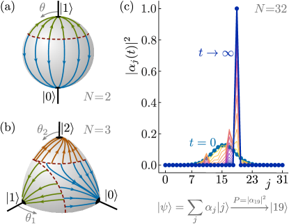
Figure 1: Dynamics of quantum state reduction. (a) The state evolution of superpositions of two pointer states as given by Eq. (4), depicted on the Bloch sphere. The pointer states form attractive fixed points of the flow on the poles of the Bloch sphere. The position of the dashed red separatrix is determined by the value of the stochastic variable $\xi$. (b) Generalization of the evolution to superpositions of three pointer states (extreme points in the flow), as given by Eq. (9). (c) Example of an initial state superposed over eight pointer states $\ket{j}$, being dynamically reduced (for a single value of the stochastic variable) to the final measurement outcome $\ket{2}$. The probability that the randomly chosen stochastic variable leads to this particular outcome is given by $P=|\alpha_{19}|^{2}$, in accordance with Born’s rule.

II Quantum state reduction from spontaneous unitarity violations

In this section, we briefly review the application of spontaneous unitarity violation to the quantum measurement problem Van Wezel (2010); Mertens et al. (2021). Following Von Neumann von Neumann (2018), we consider a strong measurement setup in which a microscopic system and macroscopic apparatus are instantaneously coupled and brought into the entangled state of Eq. (1). From here on, we will consider the joint evolution of the system and measurement device, and label their states by a single quantum number: $\ket{\psi_{i}}\equiv\ket{S_{i}}\ket{M_{i}}$. Notice that the states of the measurement apparatus in this expression are so-called pointer states Zurek (1981), which are stable under interactions with the environment. They are also states with a spontaneously broken symmetry, such as the translational symmetry broken by actual pointers. Both requirements ensure that the preferred basis in which we express the state of the measurement apparatus consists of the classical states of the apparatus observed in our everyday world. An evolution starting from the superposition of Eq. (1) and ending in a single state $\ket{\psi_{i}}$ then constitutes a description of quantum measurement.

Any theory of DQSR necessarily includes a stochastic element in order to allow for the same initial state to yield different measurement outcomes in repeated experiments Bassi et al. (2013). Furthermore, because the probability of finding any particular measurement outcome depends on the initial state, the DQSR dynamics must also necessarily be a state-dependent and thus non-linear process Mertens et al. (2021). Finally, in order to obtain irreversible single-state dynamics and stable end points of the quantum measurement process, it must be non-unitary Van Wezel (2010); Mertens et al. (2021).

A non-unitary measurement process necessarily implies the breakdown of time inversion symmetry, in the sense that the probabilistic prediction of measurement outcomes based on the initial state differs from the assignment of initial state likelihoods based on a given measurement outcome (notice the difference with time reversal symmetry: a magnet in equilibrium spontaneously breaks time reversal symmetry. The magnetized equilibrium configuration, however, is static and thus evolves the same way under time evolution forwards and backwards in time. That is, its dynamics still has time inversion symmetry). The central idea of introducing spontaneous unitarity violations (SUV), is that time inversion symmetry can be broken spontaneously, in the same way that any other symmetry of nature can be spontaneously broken. This is made possible by the infinite susceptibility of Schrödinger dynamics to even infinitesimal non-unitary perturbations in the thermodynamic limit van Wezel (2008). Assuming that unitarity is not a fundamental property of our universe, as testified for example by general relativity not being a unitary theory Penrose (1996), the diverging susceptibility to non-unitary perturbations explains the stability of (symmetry-broken) classical states for macroscopic objects van Wezel (2022). Adding a stochastic component additionally yields an objective collapse model for quantum measurement.

To be specific, consider the time evolution given by the modified Schrödinger equation:

$$i\hbar\frac{\partial|\psi(t)\rangle}{\partial t}=[\hat{H}+i\epsilon\mathcal{N}\hat{G}_{\psi(t),\xi(t)}]|\psi(t)\rangle.$$ (2)

Here $\hat{H}$ is the standard Hamiltonian acting on the joint state $\ket{\psi}$ of the microscopic system and measurement device. The unitarity-breaking perturbation is written as $\epsilon\mathcal{N}\hat{G}$, making explicit that it couples to an order parameter of the measurement device and hence scales extensively with its size $\mathcal{N}$ van Wezel (2008). Moreover, its strength $\epsilon$ is taken to be infinitesimal, so that it has negligible effect on the dynamics of microscopic systems while affecting an almost instantaneous evolution in the thermodynamic limit. The operator $\hat{G}$ is Hermitian but non-linear and depends on the state $|\psi(t)\rangle$ as well as the instantaneous value of a time-dependent stochastic variable $\xi(t)$. Together with a specification of the dynamics for $\xi(t)$, Eq. (2) describes a Markovian quantum state evolution. Notice, however, that the non-unitary dynamics describes the full state of the joint system and is not an effective model. It differs in this respect from the standard Gorini-Kossakowski-Sudarshan-Lindblad (GKSL) master equations, obtained for example by tracing out an environment in open quantum systems Lindblad (1976); Gorini et al. (1976).

In contrast to so-called continuous spontaneous localization (CSL) models Ghirardi et al. (1990), we do not assume the stochastic variable $\xi(t)$ to be Gaussian white noise, and $\xi(t)dt$ is not the infinitesimal Wiener measure $dW_{t}$ Bassi and Ghirardi (2003). Instead, we assume that the stochastic variable has a non-zero correlation time $\tau$, and we will be mostly interested in the thermodynamic limit $\mathcal{N}\to\infty$, in which the state $\ket{\psi(t)}$ evolves much faster than the stochastic variable. In that limit $\tau$ is effectively infinite and $\xi(t)$ can be taken to be a time-independent variable that is randomly chosen from a stationary distribution for each realisation of the quantum measurement process.

Specialising to the specific case of an initial state superposed over two pointer states, as in Eq. (1), we can take the Hermitian part $\hat{H}$ to be zero, because all pointer states of a good measurement device should become degenerate eigenstates of the Hamiltonian in the thermodynamic limit Beekman et al. (2019). Furthermore, the non-unitary contribution to the dynamics, $\hat{G}$, must couple to the order parameter describing the broken symmetry of the pointer state in order for the breakdown of time inversion symmetry to occur spontaneously van Wezel (2008); Van Wezel (2010). It must thus be diagonal in the pointer state basis and have different eigenvalues for different pointer states. The minimal way in which all requirements on $\hat{G}$ can be implemented is to consider:

$$\ket{\psi(t)} =\alpha(t)\ket{0}+\beta(t)\ket{1}$$

$$\hat{G}\ket{\psi(t)} =\left(\,\ket{0}\left[\frac{|\alpha(t)|^{2}-|\beta(t)|^{2}}{|\alpha(t)|^{2}+|\beta(t)|^{2}}-\xi\right]\bra{0}\right.$$

$$~{}~{}~{}+\left.\ket{1}\left[\xi-\frac{|\alpha(t)|^{2}-|\beta(t)|^{2}}{|\alpha(t)|^{2}+|\beta(t)|^{2}}\right]\bra{1}\,\right)\ket{\psi(t)}$$ (3)

In this expression, the coupling to the order parameter appears in a non-linear way, allowing the pointer states to be stable end states of the non-unitary evolution Mertens et al. (2021). The stochastic variable $\xi$ is taken from a flat, uniform distribution on the interval $[-x,x]$, with $x$ a parameter whose value will be determined below. The combination of the stochastic term in Eq. (3) being linear and its probability density function not depending on $\ket{\psi}$ ensures that, contrary to other models for DQSR, Born’s rule is not imposed in the definition of the stochastic evolution and instead has to emerge spontaneously Mertens et al. (2022).

The time evolution implied by Eqs. (2) and (3) does not conserve the norm of $\ket{\psi}$. This is not a problem as all physically observable expectation values can be defined in a norm-independent way as $\bar{O}=\bra{\psi}\hat{O}\ket{\psi}/\innerproduct{\psi}{\psi}$ Mertens et al. (2021). Alternatively, and equivalently, the time evolution can be augmented with a normalisation of the wave function either at each time step $dt$ or at the end of a period of evolution, as in other models for DQSR Bassi and Ghirardi (2003). The issue of having to define the unobservable norm and total phase can be circumvented by focusing on only the physical content of the state $\ket{\psi}$, represented by the Euler angles $\theta$ and $\varphi$ defining its representation on the Bloch sphere (see Fig 1). In fact, the relative phase $\varphi$ does not influence the evolution of $\theta$ for the time evolution generated by Eq. (3). We thus restrict attention to only the dynamics of the relative weights, given by:

$$\hbar\,{d{\theta}}/{dt}=\epsilon\mathcal{N}\sin(\theta)\left(\xi-\cos(\theta)\right)$$ (4)

Notice that the change in $\theta$ from time $t$ to $t+dt$ is completely specified by the values of $\theta$ and $\xi$ at time $t$ itself. The time evolution is thus a Markovian process without memory Bassi and Ghirardi (2003). Moreover, because the value of the stochastic variable $\xi$ is newly sampled for every realisation of the measurement process, the time evolution cannot be used for quantum state cloning, despite being non-linear Wootters and Zurek (1982); Dieks (1982).

The non-linear dynamics on the Bloch sphere defined by Eq. (4) has stable fixed points at $\theta=0$ and $\theta=\pi$, which represent the two pointer states appearing in the initial state superposition. It also has an unstable fixed line separating the attractive fixed points (a separatrix) at $\theta=\cos^{-1}(\xi)$, as shown in Fig. 1. If the value of the randomly sampled variable $\xi$ is such that the initial value $\theta(t=0)\equiv\theta_{0}$ lies above the separatrix, the state evolves towards $\theta=\pi$ under the non-unitary time evolution, while it evolves towards $\theta=0$ otherwise. The probability for ending up at either pole is thus determined by the probability for the randomly selected value $\xi$ to be smaller or larger than $\cos(\theta_{0})$. Choosing the range from which $\xi$ is sampled to be $[-1,1]$ results in final state statistics equaling Born’s rule Mertens et al. (2021, 2022). With the choice $x=1$, the time evolution of Eq. (3) thus defines a model for DQSR starting from a two-state superposition in the initial state. The spontaneous breakdown of unitarity takes place in a time scaling with $\epsilon\mathcal{N}$ so that microscopic objects take arbitrarily long to be affected by infinitesimal $\epsilon$ while the collapse process is instantaneous in the thermodynamic limit $\mathcal{N}\to\infty$, even for a vanishingly small non-unitary perturbation. Moreover, the stable end states of the quantum state reduction are given by the symmetry-breaking pointer states, and Born’s rule statistics emerge spontaneously.

III One random variable

Having a model for DQSR based on SUV for the specific case of a two-state superposition of pointer states, we will now generalize the approach to initial superpositions over $N$ pointer states. Notice the difference between $\mathcal{N}$ (the size of the measurement apparatus) and $N$ (the number of pointer states with nonzero weight in the initial superposition). The generalization can be done in multiple ways, differing in the number of required stochastic variables and the symmetry properties of the non-unitary perturbation.

The mathematically most straightforward extension of the two-state evolution can be found by first rewriting Eq. (4) in the form:

$$\hbar\,d\theta/dt=\epsilon\mathcal{N}\sin(\theta)\left(\lambda-\cos^{2}(\theta/2)\right)$$ (5)

Here, the random variable $\xi\in U[-1,1]$ was replaced with $\lambda=(\xi+1)/2$, which corresponds to a random variable taken from a uniform distribution on the domain $[0,1]$. This rewriting of the time evolution brings to the fore two important points. First, it makes clear why Born’s rule emerges. The relative weights in the two-state superposition are determined at any time by $\theta$, with pointer states corresponding to $\theta=0$ and $\theta=\pi$. If the value of $\lambda$ in Eq. (5) is lower than $\cos^{2}(\theta_{0}/2)$, then the velocity $d\theta/dt$ is negative and the value of $\theta$ will decrease, indicating an evolution towards $\theta=0$. Since $\theta$ decreases, $\lambda-\cos^{2}(\theta/2)$ will also decrease, and the sign of the velocity never changes (that is, the evolution in Fig. 1 never crosses the separatrix). Thus, for every value of $\lambda$ smaller than $\cos^{2}(\theta_{0}/2)$, the pointer state at $\theta=0$ ends up as the final outcome of the DQSR process.

The probability for finding the state $\ket{1}$ (i.e. $\theta=0$) as the result of the quantum measurement is now understood to equal the probability for the term $\lambda-|\beta_{0}|^{2}/(|\alpha_{0}|^{2}+|\beta_{0}|^{2})$ to be negative. If $\lambda$ is randomly taken from $U[0,1]$ that probability is $|\beta_{0}|^{2}/(|\alpha_{0}|^{2}+|\beta_{0}|^{2})$, in agreement with Born’s rule.

Secondly, the set of possible final states and their corresponding probabilities will not change if all diagonal elements of $\hat{G}$ are multiplied by a common factor. Such an overall multiplicative factor would affect the speed with which components evolve during the DQSR process, but not the locations of fixed points or separatrices.

Having identified these characteristics, we can propose a generalization. Consider an initial superposition over $N$ pointer states, written as:

$$\ket{\psi}=\sum_{j=0}^{N-1}{\alpha_{j}}\ket{j},~{}~{}~{}~{}\text{with}~{}~{}~{}~{}\sum_{j=0}^{N-1}\absolutevalue{\alpha_{j}}^{2}=1$$ (6)

To avoid imposing normalization at every time step, we again switch to a representation on a higher-dimensional generalization of the Bloch sphere. Introducing angles $\theta_{m}$ with $m\in\{1,2,\dots,N-1\}$ describing the relative weights of components, we write:

$$|\alpha_{N-1}| =\prod_{m=1}^{N-1}\cos\left(\frac{\theta_{m}}{2}\right)$$

$$|\alpha_{0<j<N-1}| =\sin\left(\frac{\theta_{j+1}}{2}\right)\prod_{m=1}^{j}\cos\left(\frac{\theta_{m}}{2}\right)$$

$$|\alpha_{0}| =\sin\left(\frac{\theta_{1}}{2}\right)$$ (7)

In direct analogy with the two-state process, we would like the pointer state to correspond to fixed points of the non-linear time evolution in the state-space spanned by the variables $\theta_{m}$. On the level of the evolution equation, this can is accomplished by having $d\theta_{m}/dt\propto\sin(\theta_{m})$. The flow lines then end at points in phase space where all $\theta_{m}$ equal either zero or $\pi$, or equivalently at the states $\ket{j}$ (and not superpositions of them). Notice that in fact, the state $\ket{0}$ corresponds to $\theta_{1}=\pi$, irrespective of the values of $\theta_{m}$ for $m>1$, because of the factor $\cos(\theta_{1}/2)$ appearing in all $|\alpha_{j}|$ except $|\alpha_{0}|$. Similarly, $\ket{1}$ corresponds to $\theta_{1}=0$ and $\theta_{2}=\pi$, regardless of the values of $\theta_{m}$ for $m>2$, and so on.

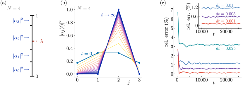
Figure 2: Quantum state reduction with one random variable. (a) The line interval $[0,1]$ can be divided into pieces with lengths corresponding to the weights $|\alpha_{j}|^{2}$ of pointer states in an initial state wave function. The probability for a stochastic variable $\lambda$ randomly chosen from a uniform distribution on $[0,1]$ to have a value corresponding to the state $\ket{j}$, is then equal to $|\alpha_{j}|^{2}$. (b) Example of an initial ($t=0$) state superposed over four pointer states $\ket{j}$, being dynamically reduced according to Eq. (9), for a particular randomly selected value of the stochastic variable, to a single measurement outcome at late times ($t\to\infty$). (c) The relative deviation from Born’s rule of the obtained distribution of final states, as a function of time for different values of the numerical time step $dt$. The relative error equals the absolute difference between $|\alpha_{j}|^{2}$ at the initial time and the fraction of simulations ending in state $\ket{j}$, summed over all $j$. In the continuum limit $dt\to 0$, the agreement with Born’s rule can be seen to become exact. These curves are for averages over the stochastic variable starting from the initial state depicted in panel (b). Similar results are obtained both for different initial state configurations, and for initial superpositions over different numbers of pointer states.

Having ensured that the possible endpoints of evolution coincide with the pointer states $\ket{j}$, we need to ensure the emergence of Born’s rule. That is, each possible final state $\ket{j}$ should have probability $|\alpha_{j}|^{2}$ of being selected by the state dynamics. This can be achieved by noticing that in a normalized state vector, the squared components of the wave function add up to one, so that we can interpret them as the lengths of line segments adding up to a line of total length one, as indicated in Fig. 2(a). The domain of the random variable $\lambda$ is $[0,1]$, so that the value of $\lambda$ can be indicated along the same line in Fig. 2(a). The probability for the value of $\lambda$ to lie within the block of size $|\alpha_{j}|^{2}$ at $t=0$ is equal to the value of $|\alpha_{j}|^{2}$ at $t=0$ itself. If the evolution ends up with the final state $\ket{j}$ whenever $\lambda$ starts out in the the block of size $|\alpha_{j}|^{2}$, Born’s rule is guaranteed to emerge.

The boundary values of $\lambda$, at which the evolutuion should switch from favouring one final state to another, are defined by:

$$\lambda =\sum_{j=0}^{n-1}|\alpha_{j}|^{2}=1-\prod_{m=1}^{n}\cos^{2}\left(\frac{\theta_{m}}{2}\right)$$ (8)

Notice that these define $N-1$ boundary values, one for each value of $n\in\{1,2,\dots,N-1\}$. They can equivalently be thought of as defining $N-1$ hypersurfaces or separatrices in the space spanned by the angles $\theta_{m}$. We will write the $N-1$ relations in Eq. (8) as $L_{n}=0$ with $L_{n}\equiv 1-\prod_{m=1}^{n}\cos^{2}(\theta_{m}/2)-\lambda$.

To define the evolution of the state, recall from Eq. (7) that the pointer state $\ket{0}$ corresponds to $\theta_{1}=\pi$, irrespective of the values of $\theta_{m}$ for $m>1$. Repeating the reasoning that led to Born’s rule in the two-state dynamics, we would thus like to see that $\theta_{1}$ increases in time and flows towards $\pi$ whenever $\lambda$ is smaller than the value of $1-\cos^{2}(\theta_{1}/2)$ at $t=0$, and opposite otherwise. That is, we should demand $d\theta_{1}/dt\propto L_{1}$.

If $\theta_{1}$ does evolve to $\pi$, Eq. (7) shows that the remainder of the evolution for the other $\theta_{m}$ can be ignored, as it does not influence the final state. In the opposite case, of $\theta_{1}$ evolving to zero, the final state will certainly not be $\ket{0}$. Given that $\theta_{1}$ will become zero, the final state will be $\ket{1}$ if $\theta_{2}$ evolves towards $\pi$, and some other state otherwise. In fact, as observed before, the state $\ket{1}$ is realised for $\theta_{2}=\pi$ regardless of the values of $\theta_{m}$ for $m>2$. If we demand $d\theta_{2}/dt\propto L_{2}$, we thus end up at the final state $\ket{1}$ if $\lambda$ is smaller than $1-\cos^{2}(\theta_{1}/2)\cos^{2}(\theta_{2}/2)$, but larger than $1-\cos^{2}(\theta_{1}/2)$ at $t=0$, establishing agreement with Born’s rule for the second component. Iterating this argument, we find that we should demand $d\theta_{n}/dt\propto L_{n}$ for all $n$.

These relations are, however, not sufficient to define the dynamics. We ensured that the hypersurface $L_{n}=0$ separates regions of opposite sign for the evolution of the parameter $\theta_{n}$, but we have not yet ascertained that the total evolution comes to a standstill at these hypersurfaces such that the evolution does not cross the newfound separatrix. In other words, we still need to force $d\theta_{n}/dt=0$ on all hypersurfaces $L_{m}$ with $m\neq n$. This can be done without affecting the sign of the evolution anywhere by demanding $d\theta_{n}/dt\propto\prod_{m\neq n}L_{m}^{2}$. Since $L_{m}$ goes to zero whenever the state state approaches the $m^{\text{th}}$ separatrix, $d\theta_{n}/dt$ is now guaranteed to go to zero at all separatrices. Moreover, since $L_{m}^{2}$ is positive on both sides of the $m^{\text{th}}$ separatrix, the sign of $d\theta_{n}/dt$ is determined solely by which side of the $n^{\text{th}}$ separatrix the state is on.

Putting everything together, we finally find that the time evolution guaranteeing Born’s rule is given by:

$$\hbar\,\frac{d\theta_{n}}{dt} =\epsilon\mathcal{N}\sin(\theta_{n})L_{n}\prod_{m\neq n}L_{m}^{2}$$

In fact, we can simplify this expression by noticing that just as in the two-state case, a single factor multiplying the time derivative of all angles does not change the fixed points or separatrices, and hence leaves the final states and their probabilities invariant. We thus absorb the common factor $\prod_{m}L_{m}^{2}$ in the definition of $\epsilon$, keeping in mind that spontaneous unitarity violations will emerge in the limit $\epsilon\to 0$, and end up with the final expression:

$$\hbar\,\frac{d\theta_{n}}{dt} =\epsilon\mathcal{N}\frac{\sin(\theta_{n})}{1-\prod_{m=1}^{n}\cos^{2}(\theta_{m}/2)-\lambda}$$ (9)

These equations define a model for DQSR starting from an $N$-state superposition in the initial state. The spontaneous breakdown of unitarity takes place in a time scaling with $\epsilon\mathcal{N}$, so that the collapse process for a vanishingly small non-unitary perturbation is effective only in the thermodynamic limit. Moreover, the stable end states of the quantum state reduction are given by the symmetry-breaking pointer states, and Born’s rule statistics emerge spontaneously in the process, using just a single random variable chosen from a state-independent, uniform distribution.

Fig. 2 shows a numerical simulation of the dynamics implied by Eq. (9). An example of a single evolution, with one value for the random variable $\lambda$, is displayed in panel 2(b), where DQSR to a single pointer state can be clearly seen. The state is normalized at each time step in order to allow visualization of the time evolution. As argued before, the normalization does not influence the final states obtained in the DQSR process, nor their probability distribution. The statistics of an ensemble of evolutions starting from the same initial state by halting each individual realisation of the dynamics whenever the relative weight of a single component exceeds a threshold value. The corresponding pointer state is then selected as the final state for that particular evolution. The deviations of the statistics from Born’s rule are shown in Fig. 2(c) to converge to zero as their numerical simulation approaches the continuum limit.

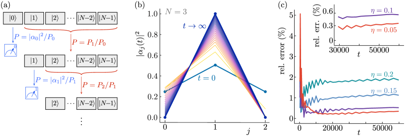
Figure 3: Quantum state reduction with $N-1$ random variables. (a) At each stage in the time evolution defined by Eq. (13), the relative weight of one component of the initial $N$-state superposition evolves to either one or zero. The different stages are separated in time by the proportionality of their evolutions to different powers of the small parameter $\eta$. (b) Example of an initial ($t=0$) state superposed over three pointer states $\ket{j}$, being dynamically reduced according to Eq. (13), for particular randomly selected values of the stochastic variables, to a single measurement outcome at late times ($t\to\infty$). (c) The relative deviation from Born’s rule of the obtained distribution of final states, as a function of time for different values of the small parameter $\eta$. The relative error equals the absolute difference between $|\alpha_{j}|^{2}$ at the initial time and the fraction of simulations ending in state $\ket{j}$, summed over all $j$. In the limit of vanishing $\eta$, the agreement with Born’s rule can be seen to become exact. These curves are for averages over the stochastic variables starting from the initial state depicted in panel (b). Similar results are obtained both for different initial state configurations, and for initial superpositions over different numbers of pointer states.

IV Multiple random variables

In the previous section, we generalized the description of SUV as a model for DQSR from initial superpositions over two pointer states to an arbitrary number of pointer states in the initial superposition. The generalization based on dividing the $N$-particle phase space into regions of attraction for the $N$ distinct pointer states is mathematically economic because it requires only a single random variable. The final form of the time evolution in Eq. (9), however, does not seem to have an obvious interpretation in terms of physical interactions. In this section and the next, we therefore introduce an alternative generalization, which more readily allows for physical interpretation. We first introduce the construction in this section, resulting in a model for DQSR of $N$-state superpositions using $N-1$ random variables. In the next section, we further refine the approach resulting in a model with $\log_{2}(N)$ random variables, which can be interpreted as components of a continuous field.

Rather than directly dividing the $N$-particle phase space into $N$ domains, we will accomplish the partitioning through a series of binary divisions. The most straightforward way to do this is to first define a time evolution that causes the weight of just one of the pointer states, say $|\alpha_{0}|=\sin(\theta_{1}/2)$ to become either zero or one:

$$\hbar\,{d\theta_{1}}/{dt} =\epsilon\mathcal{N}\sin(\theta_{1})\left(\lambda_{1}-\cos^{2}(\theta_{1}/2)\right)$$ (10)

If $\theta_{1}$ becomes $\pi$, all components $|\alpha_{j}|$ with $j$ larger than one will be zero, and Eq. (10) defines the entire DQSR process. If it evolves to zero, on the other hand, we are left with a superposition over $N-1$ pointer states. We can then define the time evolution for the next component, $|\alpha_{1}|=\sin(\theta_{2}/2)\cos(\theta_{1}/2)=\sin(\theta_{2}/2)$, so that it becomes either zero or one:

$$\hbar\,{d\theta_{2}}/{dt} =\eta\epsilon\mathcal{N}\sin(\theta_{2})\left(\lambda_{2}-\cos^{2}(\theta_{2}/2)\right)$$ (11)

Notice that we introduced a second random variable in this equation. Moreover, to ensure that the dynamics of $|\alpha_{0}|$ is effectively completed before $|\alpha_{1}|$ starts evolving, we introduced the small parameter $\eta$. In the limit $\eta\to 0$, the evolutions of the two components become independent and sequential.

This procedure can now be iterated, as illustrated in Fig. 3a, where an $N$-state system undergoes $N-1$ steps with effective two-state evolution. At each level of the partitioning, an independent stochastic component, $\lambda_{m}$ is introduced, and the evolutions are guaranteed to be independent by scaling their evolution rate with $\eta^{m}$. We then finally find the complete definition for the dynamics:

$$\hbar\,{d\theta_{m}}/{dt} =\eta^{m}\epsilon\mathcal{N}\sin(\theta_{m})\left(\lambda_{m}-\cos^{2}(\theta_{m}/2)\right)$$ (12)

Alternatively, the evolution can be specified through the generator $\hat{G}$ acting on the state $\ket{\psi}$ as defined in Eqs. (2) and (6). Its diagonal elements $G_{j}$ are then given by:

$$G_{0} =\eta^{0}\left[\frac{|\alpha_{0}|^{2}-P_{1}}{P_{0}}-\xi_{0}\right]$$

$${G}_{0<j<N-1} =\eta^{j}\left[\frac{|\alpha_{j}|^{2}-P_{j+1}}{P_{j}}-\xi_{j}\right]$$

$$+\sum_{m=0}^{j-1}\eta^{m}\left[\xi_{m}-\frac{|\alpha_{m}|^{2}-P_{m+1}}{P_{m}}\right]$$

$${G}_{N-1} =\sum_{m=0}^{N-2}\eta^{m}\left[\xi_{m}-\frac{|\alpha_{m}|^{2}-P_{m+1}}{P_{m}}\right]$$ (13)

Here, we defined $P_{m}=\sum_{j=m}^{N-1}|\alpha_{j}|^{2}$, and we reintroduced the random variables $\xi_{m}=2\lambda_{m}-1$ sampled from $U[-1,1]$. Just as in Eqs. (2) and (3), the time evolution defined by Eq. (13) is not norm-conserving. As before, this is not a problem since it does not affect any physical expectation values Mertens et al. (2021). In numerical simulations of the dynamics, however, it may be convenient to normalise the state either at the end of the calculation, or after every time step. The resulting final state is not affected by this choice.

Notice there is an (arbitrary) hierarchical structure built into the time evolution of Eq. (13). The time evolution first determines whether pointer state $\ket{0}$ will end up as the final state of the measurement process. This happens with the probability as found in the two-state evolution of Sec. II, $\sin^{2}(\theta_{1}/2)=|\alpha_{0}|^{2}$, in agreement with Born’s rule. If $\ket{0}$ is not the final state, the evolution continues, and determines whether pointer state $\ket{1}$ will be the final state. This happens with probability $\sin^{2}(\theta_{2}/2)$, but because it can only happen if $\ket{0}$ did not dominate, the total probability for state $\ket{1}$ to be the final state is $\cos^{2}(\theta_{1}/2)\sin^{2}(\theta_{2}/2)$, again in agreement with Born’s rule.

Continuing this way, the probabilities for all pointer states are seen to agree with Born’s rule. This process only works however, if the hierarchy is strictly obeyed and the evolution of $\ket{0}$ is finalised before that of $\ket{1}$ begins, and so on. This is true in the limit $\eta\to 0$, but for finite $\eta$ the final state probabilities will deviate $O(\eta)$ from Born’s rule.

The hierarchy introduced by the powers of $\eta$ that is necessary to establish Born’s rule implies an arbitrary choice for which pointer state is associated with which power of $\eta$. Although this choice does not influence the final state statistics, it does determine the finite-time dynamics and there is no clear physical reason to favour one choice over any other. In the next section, we will introduce an alternative hierarchy that results in a symmetric form of the time evolution generator, as well as a greatly reduced number of stochastic variables.

Despite these caveats, Eq. (12), or equivalently, Eq. (13), does define a model for DQSR starting from an $N$-state superposition in the initial state. The spontaneous breakdown of unitarity takes place in a time scaling with $\eta^{N-2}\epsilon\mathcal{N}$, so that the collapse process is effective for a vanishingly small non-unitary perturbation in the thermodynamic limit $\mathcal{N}\to\infty$. Moreover, the stable end states of the quantum state reduction are given by the symmetry-breaking pointer states, and Born’s rule statistics emerge spontaneously in the process, using $N$ independent random variables, each of which is chosen from a state-independent, uniform distribution.

The emergence of stable pointer states and Born’s rule can be verified numerically, as shown in figure 3. Panel 3(b) illustrates an individual instance of the time evolution generated by Eq. (12). The deviations of the statistics from Born’s rule obtained from the ensemble average over many iterations are shown in figure 3(c) to converge to zero as the hierarchy parameter $\eta$ decreases after approaching the continuum limit. Further details of the numerical simulations may be found in Appendix.A.

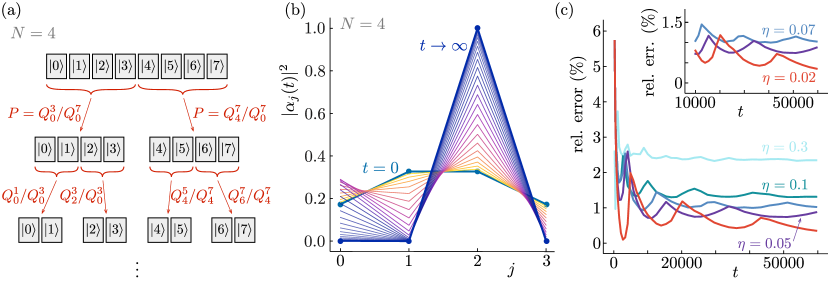
Figure 4: Quantum state reduction with $\log_{2}(N)-1$ random variables. (a) At each stage in the time evolution defined by Eq. (15), the combined relative weight of one half of the components of the initial $N$-state superposition evolves to either one or zero. At each stage a more fine-grained division of the initial pointer states is used. The different stages are separated in time by the proportionality of their evolutions to different powers of the small parameter $\eta$. (b) Example of an initial ($t=0$) state superposed over four pointer states $\ket{j}$, being dynamically reduced according to Eq. (15), for particular randomly selected values of the stochastic variables, to a single measurement outcome at late times ($t\to\infty$). (c) The relative deviation from Born’s rule of the obtained distribution of final states, as a function of time for different values of the small parameter $\eta$. The relative error equals the absolute difference between $|\alpha_{j}|^{2}$ at the initial time and the fraction of simulations ending in state $\ket{j}$, summed over all $j$. In the limit of vanishing $\eta$, the agreement with Born’s rule can be seen to become exact. These curves are for averages over the stochastic variables starting from the initial state depicted in panel (b). Similar results are obtained both for different initial state configurations, and for initial superpositions over different numbers of pointer states.

V A natural hierarchy

We will now show that the series of sequential bipartite collapse evolutions used in the previous section to construct a DQSR model based on spontaneous unitarity violations, can be organised in an alternative way. This will both be more mathematically efficient, using only $\log_{2}{N}$ random variables rather than $N-1$, and more physically appealing, as it yields a more symmetric form of the generator for time evolution that allows a natural continuum limit.

We will again consider the initial state of Eq. (6) and construct a sequence of binary collapse processes. Rather than having each process determine the fate of a single pointer state, however, each stage of the evolution suppresses the weight of half of all pointer states to zero. As shown in figure 4(a), the first stage suppresses either the weight of states $\ket{j}$ with $j=0\dots N/2-1$, or that of the states with $j=N/2\dots N-1$. In the second stage, each of these blocks has half of their states suppressed to zero weight, and subsequent stages likewise divide each of the blocks created by their predecessor.

As before, each stage in this sequential process utilizes a separate, independent random variable $\xi_{p}\in[-1,1]$, and has its time evolution scaled by a different power of the small parameter $\eta$. Because all pointer states are involved at all stages, a total of $\log_{2}(N)$ partitions suffice to single out a final state for the measurement process starting from a superposition of $N$ pointer states.

The form of the time evolution for this sequence of bipartite evolutions is most easily formulated directly in terms of the generator $\hat{G}$, rather than on the generalised Bloch sphere. To ensure the emergence of Born’s rule, the combined squared weights of half of all pointer states evolves to either zero or one during each of the stages sketched in Fig. 4(a), but the relative weights within each evolving half are not affected. We can thus directly generalise the result of Eq. (3) to write for the first stage:

$$\hat{G}^{(0)} =\sum_{j=0}^{N/2-1}\ket{j}\left[\frac{Q_{0}^{N/2-1}-Q_{N/2}^{N-1}}{Q_{0}^{N-1}}-\xi_{0}\right]\bra{j}$$

$$~{}~{}~{}~{}~{}+\sum_{j=N/2}^{N-1}\ket{j}\left[\xi_{0}-\frac{Q_{0}^{N/2-1}-Q_{N/2}^{N-1}}{Q_{0}^{N-1}}\right]\bra{j}$$ (14)

Here, we defined $Q_{m}^{n}=\sum_{j=m}^{n}|\alpha_{j}|^{2}$, and the total generator is divided into stages as $\hat{G}=\sum_{p=0}^{\log_{2}(N)-1}\hat{G}^{(p)}$, with the power of $\eta$ increasing in each consecutive stage (here, $\hat{G}^{(0)}$ implicitly includes a factor $\eta^{0}$).

Generalizing directly to the full expression, we find:

$$\hat{G}^{(p)} =\sum_{j=0}^{N-1}\ket{j}\eta^{p}\Theta(j,p)\left[\sum_{j^{\prime}=0}^{N-1}\Theta(j^{\prime},p)\frac{|\alpha_{j^{\prime}}|^{2}}{Q_{0}^{N-1}}-\xi_{p}\right]\bra{j}$$

$$\text{with}~{}~{}~{}\Theta(j,p)=(-1)^{\big{\lfloor{j2^{p+1}/N}\rfloor}}$$ (15)

Here $\lfloor{z}\rfloor$ is the floor of $z$, which equals the largest integer smaller than or equal to $z$. The value of $\Theta(j,p)$ is then either $+1$ or $-1$, and this function partitions the pointer states at each stage of the evolution.

The independence of subsequent stages in the collapse process is guaranteed by $\eta$ being a small parameter, as in the previous section. Since Born’s rule was shown to emerge in the two-state process of Eq. (3), it is also guaranteed to emerge from Eq. (15) in the limit of vanishing $\eta$. For finite values of $\eta$, deviations from Born’s rule of order $\eta$ will occur.

Equation (15) is one of the main results of this article. It defines a model for DQSR starting from an $N$-state superposition in the initial state. The spontaneous breakdown of unitarity takes place in a time scaling with $\eta^{\log_{2}(N)}\epsilon\mathcal{N}$, so that the collapse process is effective for a vanishingly small non-unitary perturbation in the thermodynamic limit $\mathcal{N}\to\infty$. The stable end states of the quantum state reduction are given by the symmetry-broken pointer states, and Born’s rule statistics emerge spontaneously in the process, using $\log_{2}(N)$ independent random variables, each of which is chosen from a state-independent, uniform distribution. Moreover, despite the hierarchy of the collapse process, the form of Eq. (15) is symmetric in the sense that all pointer states evolve during all stages of the DQSR process.

The division of pointer states into two groups at each stage can be interpreted as a stepwise fine-graining of the measurement outcome. Since pointer states correspond to classical symmetry-broken states of matter, they differ in the value or direction of an order parameter Beekman et al. (2019); Van Wezel (2010). For an actual pointer along a dial, for example, this could be the position of the tip of the pointer. This means there is a natural ordering of pointer states, in the order parameter space. The states of an actual pointer, for example, could be ordered in real space, going from one end of the dial to the other. Within this natural ordering, the first stage of the DQSR process described by Eq. (15) then suppresses one connected set of pointer states, establishing that the measurement outcome will fall within the remaining half. The second stage suppresses a connected section of the remaining states and establishes the quarter of all initial states among which the final state will fall. Continuing this way, each consecutive stage of the process gives a more fine-grained set of candidates for the final state. This interpretation of fine-graining in an order parameter space suggests a natural continuum limit for Eq. (15), which we will explore in the following section.

The emergence of stable pointer states and Born’s rule can again be verified numerically, as shown in Fig. 4. Panel 4(b) illustrates an individual instance of the time evolution generated by Eq. (15). The deviations of the statistics from Born’s rule obtained from the ensemble average over many iterations are shown in fig. 4(c) to converge to zero as the hierarchy parameter $\eta$ decreases after approaching the continuum limit. Further details of the numerical simulations may be found in Appendix.A.

VI Towards a random field

The final form of the DQSR process with $\log_{2}(N)$ random variables in Eq. (15) suggests a natural generalization to a model for quantum measurement with the initial state superposed over a continuous set of states. Without loss of generality, consider a line segment parameterized by the coordinate $x\in[0,1]$. The initial state is now:

$$\ket{\psi}=\int_{0}^{1}dx\,\psi(x)\ket{x}~{}~{}~{}\text{with}~{}~{}~{}\int_{0}^{1}dx\,\absolutevalue{\psi(x)}^{2}=1$$ (16)

Taking the discrete pointer states $\ket{j}$ of the previous section to lie within the continuous interval parameterized by $x$ and taking the continuum limit $N\to\infty$ after identifying $x=j/N$, the contribution to the time evolution generator at stage $p$ becomes:

$$\hat{G}^{(p)} =\int_{0}^{1}dx\,\ket{x}\eta^{p}\theta(x,p)~{}\times$$

$$~{}~{}~{}~{}~{}~{}~{}~{}~{}\left[\int_{0}^{1}dx^{\prime}\,\theta(x^{\prime},p)\frac{|\psi(x^{\prime})|^{2}}{Q}-\xi(p)\right]\bra{x}$$ (17)

Here, we introduced the generally time-dependent norm $Q(t)=\int_{0}^{1}dx\,|\psi(x,t)|^{2}$ as well as the continuum version of the sign distribution function on the interval $[0,1]$, given by $\theta(x,p)=(-1)^{\big{\lfloor{x2^{p+1}}\rfloor}}$. The full generator is given by $\hat{G}=\sum_{p=0}^{\gamma}\hat{G}^{(p)}$, with $\gamma$ an ultraviolet cutoff.

The full time evolution generator can be cast in a more suggestive form by defining:

$$\hat{G}\ket{\psi}=\int_{0}^{1}dx\,G(x)\psi(x)\ket{x}$$ (18)

The non-linear components of $\hat{G}$ are then given by:

$$G(x) =\Lambda(x)+\int_{0}^{1}dx^{\prime}\,\frac{\absolutevalue{\psi(x^{\prime})}^{2}}{Q}\Pi(x,x^{\prime})$$

$$=\Lambda(x)+\left<\hat{\Pi}(x)\right>.$$ (19)

The expectation value $\langle\hat{\Pi}(x)\rangle$ resembles a spatial propagator with elements $\Pi(x,x^{\prime})=\sum_{0}^{\gamma}\eta^{p}\,\theta(x,p)\theta(x^{\prime},p)$, while $\Lambda(x)=-\sum_{0}^{\gamma}\eta^{p}\xi_{p}\theta(x,p)$ represents the value at location $x$ of a random field on the line segment $[0,1]$. Because the stages labeled by $p$ represent different levels of fine-graining in the $x$-space resolution of the final pointer state, the ultra-violet cut-off $\gamma$ also defines a minimum separation for which points along the $[0,1]$ line segment can be resolved. If the pointer states break a symmetry corresponding to an order parameter labeled by a real-space coordinate (such as an actual pointer along a dial), the ultraviolet cutoff could for example be set by the Planck length. Measurement outcomes can then only ever be resolved down to Planck length precision, and the random field $\Lambda(x)$ takes independent random values on positions separated by a Planck length.

VII Conclusions

In conclusion, we constructed several models for dynamic quantum state reduction based on the idea that the time inversion symmetry underlying unitarity in quantum dynamics can be spontaneously broken, like any other symmetry in nature. Although it has been known for some time that the unitary dynamics of Schrödinger’s equation is unstable in the thermodynamic limit van Wezel (2008); Van Wezel (2010), a concrete model for the unitarity-breaking time evolution starting from a generic initial state and obeying all requirements for a model of quantum measurement was still lacking. Here, we showed that the measurement dynamics previously proposed for an initial superposition over two pointer states Mertens et al. (2021) can be generalized to arbitrary initial states in several ways, which differ in the way Born’s rule emerges during the measurement process.

We first considered a mathematically straightforward generalization, in which just a single random variable chosen from a flat, uniform distribution leads to precisely Born’s rule for an initial superposition of an arbitrary finite number of pointer states. This model, however, does not have a straightforward physical interpretation.

Next, we constructed a generalization using as many random variables as there are pointer states (minus one) in the initial superposition. The emergence of Born’s rule in this model relies on the presence of separate stages in the measurement dynamics and is perfect only in the limit of vanishing overlap between these stages. Moreover, the model requires the introduction of an arbitrary hierarchy among the pointer states.

The final generalization we introduced removes the arbitrary hierarchy and replaces it with a natural ordering of the pointer states interpreted as symmetry-breaking states with a macroscopic order parameter. This way, only $\log_{2}(N)$ random variables are required to model the dynamical quantum state reduction of an initial superposition over $N$ pointer states. Moreover, the final generator for time evolution in the model has a natural continuum limit, which can be interpreted in terms of a random field in real space and an expectation value resembling a real-space propagator.

The final model for the state reduction dynamics meets all requirements for a model of quantum measurement: its origin in a theory for spontaneous unitarity violation implies that it has no effect on the microscopic scale of elementary particles, even though it dominates the behavior of macroscopic, everyday objects and causes them to collapse instantaneously in the thermodynamic limit. The final states in that collapse process are the symmetry-breaking pointer states that we associate with real-world measurement machines, and after one of them has been selected in the stochastic measurement dynamics, it remains stable. Finally, the probability of finding any particular final state is given by Born’s rule, which emerges spontaneously without being used, assumed, or imposed in the definition of the stochastic field.

The models presented here explicitly demonstrate the possibility of spontaneous unitarity violations giving rise to DQSR dynamics in a way that obeys all basic requirements for a theory of quantum measurement. The models can be extended in several directions, including for example by formulating a field theory in Fock space, or by generalizing the basis of sign functions appearing in the continuum model. We hope the present work will inspire and lay the foundation for further proposals of dynamic quantum state reduction based on spontaneous unitarity violation. These may find application in describing the dynamics of (quantum) phase transitions van Wezel (2022); Beekman et al. (2019) as well as quantum measurement, yield testable experimental predictions Wezel and Oosterkamp (2011), and generally shed new light on the crossover regime separating Schrödinger from Newtonian dynamics.

Acknowledgement

The authors gratefully acknowledge stimulating discussions with J. Zaanen on the role of two-fold partitions in the time evolution operator.

Appendix A Numerical simulations

In this appendix we describe the numerical simulations leading to Figs. 2(b, c), 3(b, c) and 4(b, c). Convergence in the numerical integration of Eqs. (9), (13), and (15) is obtained using sufficiently small time steps $dt$. In Fig. 2(c) we show convergence to Born rule statistics for decreasing value of the time step. The dynamics defined in Secs. IV and V additionally require a small hierarchical parameter $\eta$. For any given value of $\eta$ the size of $dt$ was adjusted to ensure convergent results, with lower values of $\eta$ requiring smaller time steps. Therefore, in Fig. 3(c), the values $\eta=0.05$ and $dt=0.005$ were used, while for other values of $\eta$ taking $dt=0.01$ sufficed. The results in Fig. 4(c) used $dt=0.01$ for all cases except for $\eta=0.05$ and $\eta=0.02$, which both utilized $dt=0.005$.

To recover Born rule statistics, a numerical average must be taken over a dense and uniform set of values for the stochastic variable. The results in Fig. 2(c) represent averages over $100$ to approximately $25000$ values for the stochastic variable, while up to $60000$ values were sampled in the creation of Figs. 3(c) and 4(c).

Appendix B Continuum distributions

In this appendix, we discuss the functions $\Theta(x,p)$ and $\Lambda(x)$ emerging in the continuum theory of Sec. VI. The sign distribution function $\Theta(x,p)$ is defined as $(-1)^{\lfloor{x2^{p+1}}\rfloor}$ with $x\in[0,1]$. It shown for the first four values of the discrete parameter $p$ in Fig. B.1(b). For any given value of $p$, the function $\Theta(x,p)$ is a square wave, with values alternating between $1$ and $-1$. Notice that any real function on a discrete lattice can be decomposed into these square wave components, much like a Fourier decomposition. To decompose continuous functions, a regularization of the limiting function at $p\to\infty$ will be required.

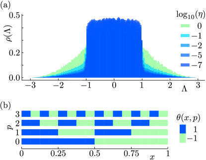
Figure B.1: (a) The probability distribution function for the random value $\Lambda(x)$, for arbitrary $x$, obtained by numerically averaging over $50000$ randomly selected values for the stochastic variables $\xi_{p}$. The results for different values of the small parameter $\eta$ converge to a uniform distribution on the interval $[-1,1]$ for vanishing $\eta$. (b) Schematic depiction of the function $\theta(x,p)$, for the continuous variable $x\in[0,1]$ and $p$ discrete.

Finally, the stochastic field $\Lambda(x)$ was defined in Sec. VI as $-\sum_{0}^{\gamma}\eta^{p}\xi_{p}\theta(x,p)$. The probability density function for $\Lambda(x)$ will be independent of $x$, since it is given by a sum over stochastic variables with coefficients that differing by at most a sign. The probability density function resulting from a numerical evaluation of the sum for $50000$ samples of the random parameters is displayed in Fig. B.1(a), for an arbitrary value of $x$. It corresponds to a type of truncated Gaussian-like distribution for large values of $\eta$, while converging to uniform distribution with tapering edges for smaller values of $\eta$. The tapering at the edges is suppressed as $\eta$ is increased, and the probability density function approaching a true uniform distribution, $U[-1,1]$, as $\eta$ approaches zero.

References

- Bassi and Ghirardi (2003) A. Bassi and G. Ghirardi, Physics Reports (2003), 10.1016/s0370-1573(03)00103-0.
- Leggett (2005) A. Leggett, science 307, 871 (2005).
- Bassi et al. (2013) A. Bassi, K. Lochan, S. Satin, T. P. Singh, and H. Ulbricht, Rev. of mod. phys 85, 471–527 (2013).
- Arndt and Hornberger (2014) M. Arndt and K. Hornberger, Nature Physics 10, 271 (2014).
- Carlesso et al. (2022) M. Carlesso, S. Donadi, L. Ferialdi, M. Paternostro, H. Ulbricht, and A. Bassi, Nature Physics 18, 243 (2022).
- Born (1926) M. Born, Zeitschrift fur Physik 38, 803 (1926).
- von Neumann (2018) J. von Neumann, in Mathematical Foundations of Quantum Mechanics, edited by N. A. Wheeler (Princeton University Press, 2018).
- Arndt et al. (1999) M. Arndt, O. Nairz, J. Vos-Andreae, C. Keller, G. van der Zouw, and A. Zeilinger, Nature (1999), 10.1038/44348.
- Hackermüller et al. (2003) L. Hackermüller, S. Uttenthaler, K. Hornberger, E. Reiger, B. Brezger, A. Zeilinger, and M. Arndt, Phys. Rev. Lett. (2003), 10.1103/physrevlett.91.090408.
- Gerlich et al. (2011) S. Gerlich, S. Eibenberger, M. Tomandl, S. Nimmrichter, K. Hornberger, P. J. Fagan, P. J. Fagan, J. Tüxen, M. Mayor, and M. Arndt, Nature Communications (2011), 10.1038/ncomms1263.
- Gasbarri et al. (2021) G. Gasbarri, A. Belenchia, M. Carlesso, M. Carlesso, S. Donadi, A. Bassi, R. Kaltenbaek, M. Paternostro, and H. Ulbricht, Communications in Physics (2021), 10.1038/s42005-021-00656-7.
- Zurek (1982) W. H. Zurek, Phys. Rev. D (1982), 10.1103/physrevd.26.1862.
- Schlosshauer (2005) M. Schlosshauer, Reviews of Modern Physics (2005), 10.1103/revmodphys.76.1267.
- Zurek (2009) W. H. Zurek, Nature Physics 5, 181 (2009).
- Allahverdyan et al. (2013) A. E. Allahverdyan, R. Balian, and T. M. Nieuwenhuizen, Physics Reports 525, 1 (2013).
- Dieks (1989) D. Dieks, Physics Lett. A (1989), 10.1016/0375-9601(89)90510-0.
- Adler (2003) S. L. Adler, Stud. Hist. Phil. Science B 34, 135 (2003).
- von Stillfried (2008) N. von Stillfried, Nature (2008), 10.1038/453978c.
- Fortin and Lombardi (2014) S. Fortin and O. Lombardi, Foundations of Physics 44, 426 (2014).
- Everett (1957) H. Everett, Reviews of Modern Physics (1957), 10.1103/revmodphys.29.454.
- Bohm (1952a) D. Bohm, Phys. Rev. 85, 166 (1952a).
- Bohm (1952b) D. Bohm, Phys. Rev. 85, 180 (1952b).
- Rovelli (1996) C. Rovelli, International Journal of Theoretical Physics 35, 1637 (1996).
- Fuchs et al. (2014) C. A. Fuchs, N. D. Mermin, R. Schack, and R. Schack, American Journal of Physics (2014), 10.1119/1.4874855.
- Bohm and Bub (1966) D. Bohm and J. Bub, Rev. Mod. Phys. 38, 453 (1966).
- Pearle (1976) P. Pearle, Phys. Rev. D (1976), 10.1103/physrevd.13.857.
- Gisin (1984) N. Gisin, Phys. Rev. Lett. 52, 1657 (1984).
- Ghirardi et al. (1986) G. Ghirardi, A. Rimini, and T. Weber, Phys. Rev. D (1986), 10.1103/physrevd.34.470.
- Diósi (1987) L. Diósi, Physics Lett. A (1987), 10.1016/0375-9601(87)90681-5.
- Ghirardi et al. (1990) G. Ghirardi, P. Pearle, and A. Rimini, Phys. Rev. A (1990), 10.1103/physreva.42.78.
- Percival (1995) I. C. Percival, Proceedings of the Royal Society of London. Series A: Mathematical and Physical Sciences 451, 503 (1995).
- Penrose (1996) R. Penrose, General Relativity and Gravitation (1996), 10.1007/bf02105068.
- Van Wezel (2010) J. Van Wezel, Symmetry 2, 582 (2010).
- Marshall et al. (2003) W. Marshall, C. Simon, R. Penrose, and D. Bouwmeester, Phys. Rev. Lett. 91, 130401 (2003).
- Donadi et al. (2020) S. Donadi, K. Piscicchia, C. Curceanu, L. Diósi, M. Laubenstein, and A. Bassi, Nature Physics (2020), 10.1038/s41567-020-1008-4.
- Vinante et al. (2017) A. Vinante, R. Mezzena, P. Falferi, M. Carlesso, and A. Bassi, Phys. Rev. Lett. 119 (2017), 10.1103/physrevlett.119.110401.
- Carlesso et al. (2016) M. Carlesso, A. Bassi, P. Falferi, and A. Vinante, Phys. Rev. D 94 (2016), 10.1103/physrevd.94.124036.
- Mertens et al. (2021) L. Mertens, M. Wesseling, N. Vercauteren, A. Corrales-Salazar, and J. van Wezel, Phys. Rev. A 104, 052224 (2021).
- Mertens et al. (2022) L. Mertens, M. Wesseling, and J. van Wezel, (2022), arXiv:quant-ph/2208.11584 .
- Zurek (1981) W. H. Zurek, Phys. Rev. D 24, 1516–1525 (1981).
- van Wezel (2008) J. van Wezel, Phys. Rev. B 78, 054301 (2008).
- van Wezel (2022) J. van Wezel, J. Phys. A: Math. Theor. 55, 401001 (2022).
- Lindblad (1976) G. Lindblad, Commun. Math. Phys. 48, 119 (1976).
- Gorini et al. (1976) V. Gorini, A. Kossakowski, and E. C. G. Sudarshan, J. Math. Phys. 17, 821 (1976).
- Beekman et al. (2019) A. J. Beekman, L. Rademaker, and J. van Wezel, SciPost Phys. Lect. Notes 11 (2019), 10.21468/SciPostPhysLectNotes.11.
- Wootters and Zurek (1982) W. K. Wootters and W. H. Zurek, Nature (1982), 10.1038/299802a0.
- Dieks (1982) D. Dieks, Physics Letters A 92, 271 (1982).
- Wezel and Oosterkamp (2011) J. V. Wezel and T. H. Oosterkamp, Proceedings of the Royal Society A: Mathematical, Physical and Engineering Sciences 468, 35–56 (2011).