COMBINATORIAL PROPERTIES FOR A CLASS OF SIMPLICIAL COMPLEXES EXTENDED FROM PSEUDO-FRACTAL SCALE-FREE WEB

Abstract

Simplicial complexes are a popular tool used to model higher-order interactions between elements of complex social and biological systems. In this paper, we study some combinatorial aspects of a class of simplicial complexes created by a graph product, which is an extension of the pseudo-fractal scale-free web. We determine explicitly the independence number, the domination number, and the chromatic number. Moreover, we derive closed-form expressions for the number of acyclic orientations, the number of root-connected acyclic orientations, the number of spanning trees, as well as the number of perfect matchings for some particular cases.

1 INTRODUCTION

Complex networks have become a popular and powerful formalism for describing diverse types of real-world complex interactive systems in nature and society, whose nodes and edges represent, respectively, the elements and their interactions in real systems [1]. In a large majority of previous studies [2], the authors consider only pairwise interactions between elements in complex systems, overlooking other interactions such as higher-order ones among multiple elements. Some recent works [3, 4, 5, 6, 7] demonstrate that many real-life systems involve not only dyadic interactions but also interactions among more than two elements at a time. Such multi-way interactions among elements are usually called higher-order interactions or simplicial interactions. For example, in a scientific collaboration network [8], for a paper with more than two authors, the interactions among the authors are not pairwise but higher-order. Similar higher-order interactions are also ubiquitous in neuronal spiking activities [9, 10], proteins [11], and other real-life systems.

Since the function and various dynamics of a complex system rely to a large extent on the way of interactions between its elements, it is expected that higher-order interactions have a substantial impact on collective dynamics of complex systems with simplicial structure. The last several years have seen some important progress about profound influences of higher-order interactions on different dynamical processes [12], including percolation [13], public goods game [14], synchronization [15, 16], and epidemic spreading [17]. For example, in comparison with pairwise interactions, three-way interactions can lead to many novel phenomena, such as Berezinkii-Kosterlitz-Thouless percolation transition [13], abrupt desynchronization [15], as well as abrupt phase transition of epidemic spreading [17].

In order to describe the widespread higher-order interactions observed in various real-world complex systems, a lot of models have been proposed [12], based on some popular mathematical tools, such as simplicial complexes [18, 19, 7, 20]. A simplex of dimension $d$, called $d$-simplex, represents a single high-order interaction among $d+1$ nodes [21], which can be described by a complete graph of $d+1$ nodes. For example, a $0$-simplex is a node, a $1$-simplex is a link, a $3$-simplex is a triangle, while a $4$-simplex is a tetrahedron. For a $d$-simplex $\alpha$, a $\delta$-dimensional face $\alpha^{\prime}$ of $\alpha$ is a $\delta$-simplex with $0\leqslant\delta<d$ formed by a subset of the nodes in $\alpha$, i.e., $\alpha^{\prime}\subseteq\alpha$. For instance, the faces of a $4$-simplex include four nodes, six links, and four triangles. A simplicial complex is a collection of simplices, which is formed by simplices glued along their faces. A simplicial complex is called $d$-dimensional if its constituent simplices are those of dimension at most $d$. Thus, simplicial complexes describe higher-order interactions in a natural way.

Most of existing models are stochastically, which makes it a challengeable task to exactly analyze their topological and dynamical properties. Very recently, leveraging the edge corona product of graphs [22, 23], a family of iteratively growing deterministic network model was developed [24, 25] to describe higher-order interactions. They are called deterministic simplicial networks, since they are consist of simplexes. This network family subsumes the pseudo-fractal scale-free web [26] as a particular case, which has received considerable attention from the scientific community, including fractals [27, 28, 29], physics [30, 31, 32, 33, 34, 35], and cybernetics [36, 37]. The deterministic construction allow to study exactly at least analytically relevant properties: They display the remarkable scale-free [38] and small-world [39] properties that are observed in most real-world networks [1], and all the eigenvalues and their multiplicities of their normalized Laplacian matrices can be exactly determined [24].

Although some structural and algebraic properties for the deterministic simplicial networks have been studied, their combinatorial properties are less explored or not well understood. In this paper, we present an in-depth study on several combinatorial problems for deterministic simplicial networks. Our main contributions are as follows. We first provide an alternative construction of the networks, which shows that the networks are self-similar. We then determine explicitly the domination number, the independence number, as well as the chromatic matching number. Finally, we provide exact formulas for the number of acyclic orientations, the number of root-connected acyclic orientations, the number of spanning trees, and the number of perfect matchings for some special cases. Our exact formulae for the independence number, the domination number, and the number of spanning trees generalize the results [40, 41, 33] previously obtained for the pseudo-fractal scale-free web.

The main reasons for studying the above combinatorial problems lie in at least two aspects. The first one is their inherent theoretical interest [42, 43, 44, 45], because it is a theoretical challenge to solve these problems. For example, counting all perfect matchings in a graph is #P-complete [46, 47]. In view of the hardness, Lovász [48] pointed out that it is of great interest to construct or find special graphs for which these combinatorial problems can be exactly solved. The deterministic simplicial networks are in such graph category. The other justification lies in the relevance of the studied combinatorial problems to practical applications. For example, minimum dominating sets [49] and maximum matchings [50] can be applied to study structural controllability of networks [51], while maximum independent set problem is closely related to graph data mining [52, 53]. Thus, our work provides useful insight into understanding higher-order structures in the application scenarios of these combinatorial problems.

2 NETWORK CONSTRUCTIONS AND PROPERTIES

The family of simplicial networks under consideration was proposed in [24], which is constructed based on the edge corona product of graphs [22, 23]. Let $\mathcal{G}_{1}$ and $\mathcal{G}_{2}$ be two graphs with disjoint node sets, where $\mathcal{G}_{1}$ have $n_{1}$ nodes and $m_{1}$ edges. The edge corona product $\mathcal{G}_{1}\circledcirc\mathcal{G}_{2}$ of $\mathcal{G}_{1}$ and $\mathcal{G}_{2}$ is a graph obtained by taking one replica of $\mathcal{G}_{1}$ and $m_{1}$ replicas of $\mathcal{G}_{2}$, and connecting both end nodes of the $i$-th edge of $\mathcal{G}_{1}$ to every node in the $i$-th replica of $\mathcal{G}_{2}$ for $i=1,2,\ldots,m_{1}$. Let $\mathcal{K}_{q}$ ($q\geqslant 1$) denote the $q$-node complete graph, with $\mathcal{K}_{1}$ being a graph with an isolate node. Let $\mathcal{G}_{q}(g)=(\mathcal{V}(\mathcal{G}_{q}(g)),\mathcal{E}(\mathcal{G}_{q}(g)))$ denote the studied networks after $g$ iterations, where $\mathcal{V}(\mathcal{G}_{q}(g))$ and $\mathcal{E}(\mathcal{G}_{q}(g))$ are the sets of nodes and edges, respectively. Then, $\mathcal{G}_{q}(g)$ is constructed as follows, controlled by two parameters $q$ and $g$ with $q\geqslant 1$ and $g\geqslant 0$.

Definition 2.1.

For $g=0$, $\mathcal{G}_{q}(0)$ is the complete graph $\mathcal{K}_{q+2}$. For $g\geqslant 0$, $\mathcal{G}_{q}(g+1)$ is obtained from $\mathcal{G}_{q}(g)$ by performing the following operation: for every existing edge of $\mathcal{G}_{q}(g)$, one creates a copy of the complete graph $\mathcal{K}_{q}$ and connects all its $q$ nodes to both end nodes of the edge. That is, $\mathcal{G}_{q}(g+1)=\mathcal{G}_{q}(g)\circledcirc\mathcal{K}_{q}$.

Figure 2 illustrates the operation obtaining $\mathcal{G}_{q}(g+1)$ from $\mathcal{G}_{q}(g)$, while Fig. 2.1 illustrates the network construction processes for two cases of $q=1$ and $q=2$.

Network construction approach. For each existing edge in network $\mathcal{G}_{q}(g)$, performing the operation on the right-hand side of the arrow generates network $\mathcal{G}_{q}(g+1)$. The filled circles stand for the nodes constructing the complete graph $\mathcal{K}_{q}$, and all the filled circles which appeared in step $g+1$ link to both end open nodes of the edge that already exist in the previous step $g$.

The first several iterations of $\mathcal{G}_{q}(g)$ for $q=1$ and $2$. The nodes generated at different iterations are marked with different colors.

Let $N_{g,q}=|\mathcal{V}(\mathcal{G}_{q}(g))|$ and $M_{g,q}=|\mathcal{E}(\mathcal{G}_{q}(g))|$ denote, respectively, the number of nodes and the number of edges in $\mathcal{G}_{q}(g)$. By construction, one obtains the following recursion relations for $M_{g,q}$ and $N_{g,q}$:

$$M_{g+1,q}=\frac{(q+1)(q+2)}{2}M_{g,q}$$ (1)

and

$$N_{g+1,q}=q\,M_{g,q}+N_{g,q},$$ (2)

which, together with $N_{0,q}=q+2$ and $M_{0,q}=(q+1)(q+2)/2$, lead to

$$M_{g,q}={\left[\frac{(q+1)(q+2)}{2}\right]}^{g+1}$$ (3)

and

$$N_{g,q}=\frac{2}{q+3}{\left[\frac{(q+1)(q+2)}{2}\right]}^{g+1}+\frac{2(q+2)}{q+3}.$$ (4)

Thus, the average degree of nodes in graph $\mathcal{G}_{q}(g)$ is $2M_{g,q}/N_{g,q}$, which tends to $q+3$ when $g$ is large, implying that $\mathcal{G}_{q}(g)$ is sparse.

For graph $\mathcal{G}_{q}(g)$, let $\mathcal{W}_{q}(g)=\mathcal{V}(\mathcal{G}_{q}(g))\backslash\mathcal{V}(\mathcal{G}_{q}(g-1))$ represent the set of new nodes generated at iteration $g$. Then,

$$|\mathcal{W}_{q}(g)|=q\left[\frac{(q+1)(q+2)}{2}\right]^{g}.$$ (5)

Let $d^{(g,q)}_{v}$ denote the degree of node $v$ in graph $\mathcal{G}_{q}(g)$, which was created at iteration $g_{v}$. Then, $d^{(g,q)}_{v}=(q+1)^{g-g_{v}+1}$. It is easy to verify that in graph $\mathcal{G}_{q}(g)$, there are $q+2$ nodes with degree $(q+1)^{g+1}$ and $q\left[\frac{(q+1)(q+2)}{2}\right]^{t_{v}}$ nodes with degree $(q+1)^{g-g_{v}+1}$ for $0<t_{v}<g$.

In graph $\mathcal{G}_{q}(g)$, the $q+2$ nodes with the highest degree $(q+1)^{g+1}$ are called hub nodes, which are generated at the initial interaction $g=0$. Let $h_{k}(g)$, $k=1,2,\ldots,q+2$, denote the $q+2$ hub nodes of graph $\mathcal{G}_{q}(g)$, and let $\mathcal{V}_{\rm h}(\mathcal{G}_{q}(g))$ denote the set of these hub nodes, that is, $\mathcal{V}_{\rm h}(\mathcal{G}_{q}(g))=\{h_{1}(g),h_{2}(g),\ldots,h_{q+2}(g)\}$. Then, the simplicial networks can be generated in an alternative way, highlighting the self-similarity.

Proposition 2.2.

Given graph $\mathcal{G}_{q}(g)$, graph $\mathcal{G}_{q}(g+1)$ can be obtained by joining $\frac{(q+1)(q+2)}{2}$ copies of $\mathcal{G}_{q}(g)$, denoted as $\mathcal{G}_{q}^{(i,j)}(g)$ $(1\leq i<j\leq q+2)$, the $k$-th $(k=1,2,\ldots,q+2)$ hub node of which is denoted by $h_{k}^{(i,j)}(g)$. Concretely, in the merging process, for each $k=1,2,\ldots,q+2$, the $q+1$ hub nodes $h_{k}^{(1,k)}(g)$, $h_{k}^{(2,k)}(g)$, $\ldots$, $h_{k}^{(k-1,k)}(g)$, $h_{k}^{(k,k+1)}(g)$, $\ldots$, $h_{k}^{(k,q+2)}(g)$ in the corresponding replicas of $\mathcal{G}_{q}(g)$ are identified as the hub node $h_{k}(g+1)$ of $\mathcal{G}_{q}(g+1)$.

Proof 2.3.

We prove this proposition by induction on $g$. For $g=0$, the proof is trivial. For $g>0$, assume that the conclusion holds for $\mathcal{G}_{q}(g)$, i.e: $\mathcal{G}_{q}(g)$ can be obtained as joining $\frac{(q+1)(q+2)}{2}$ copies of $\mathcal{G}_{q}(g-1)$, which are denoted by $\mathcal{G}_{q}^{(i,j)}(g-1)$ with $1\leq i<j\leq q+2$. During the amalgamation process, for each $k\in\{1,2,\ldots,q+2$}, the $q+1$ hub nodes $h_{k}^{(1,k)}(g-1)$, $h_{k}^{(2,k)}(g-1)$, $\ldots$, $h_{k}^{(k-1,k)}(g-1)$, $h_{k}^{(k,k+1)}(g-1)$, $\ldots$, $h_{k}^{(k,q+2)}(g-1)$ in the corresponding $q+1$ replicas of $\mathcal{G}_{q}(g-1)$ are identified as the hub node $h_{k}(g)$ of $\mathcal{G}_{q}(g)$. For convenient description, we use

$$\mathcal{G}_{q}(g)= \textbf{J}\big{[}\mathcal{G}_{q}^{(1,2)}(g-1),\mathcal{G}_{q}^{(1,3)}(g-1),\ldots,$$

$$\mathcal{G}_{q}^{(1,q+2)}(g-1),\ldots,\mathcal{G}_{q}^{(q+1,q-1)}(g-1),$$

$$\mathcal{G}_{q}^{(q+1,q+2)}(g-1);\mathcal{V}_{\rm h}(\mathcal{G}_{q}(g))\big{]},$$

to denote the above process merging $\mathcal{G}_{q}^{(i,j)}(g-1)$ ($1\leq i<j\leq q+2$) to $\mathcal{G}_{q}(g)$, where $\mathcal{V}_{\rm h}(\mathcal{G}_{q}(g)))$ is the set of the $q+2$ hub nodes in $\mathcal{G}_{q}(g)$, which are identified from the hub nodes in the $\frac{(q+1)(q+2)}{2}$ copies $\mathcal{G}_{q}^{(i,j)}(g-1)$ of $\mathcal{G}_{q}(g-1)$.

Next we will prove that the conclusion holds for $\mathcal{G}_{q}(g+1)$. Note that for any graph $\mathcal{G}$ with the degree of its hub nodes larger than 1, $\mathcal{V}_{\rm h}(\mathcal{G}\circledcirc\mathcal{K}_{q})=\mathcal{V}_{\rm h}(\mathcal{G})$. By Definition 2.1, $\mathcal{G}_{q}(g+1)=\mathcal{G}_{q}(g)\circledcirc\mathcal{K}_{q}$. Thus, using the definition of edge corona product and inductive hypothesis, we have

$$\quad\mathcal{G}_{q}(g+1)=\mathcal{G}_{q}(g)\circledcirc\mathcal{K}_{q}$$

$$=\textbf{J}\big{[}\mathcal{G}_{q}^{(1,2)}(g-1),\mathcal{G}_{q}^{(1,3)}(g-1),\ldots,$$

$$\quad\mathcal{G}_{q}^{(q+1,q+2)}(g-1);\mathcal{V}_{\rm h}(\mathcal{G}_{q}(g))\big{]}\circledcirc\mathcal{K}_{q}$$

$$=\textbf{J}\big{[}\mathcal{G}_{q}^{(1,2)}(g-1)\circledcirc\mathcal{K}_{q},\mathcal{G}_{q}^{(1,3)}(g-1)\circledcirc\mathcal{K}_{q},\ldots,$$

$$\quad\mathcal{G}_{q}^{(q+1,q+2)}(g-1)\circledcirc\mathcal{K}_{q};\mathcal{V}_{\rm h}(\mathcal{G}_{q}(g))\big{]}$$

$$=\textbf{J}\big{[}\mathcal{G}_{q}^{(1,2)}(g),\mathcal{G}_{q}^{(1,3)}(g),\ldots,\mathcal{G}_{q}^{(q+1,q+2)}(g);$$

$$\quad\mathcal{V}_{\rm h}(\mathcal{G}_{q}(g))\big{]}$$

$$=\textbf{J}\big{[}\mathcal{G}_{q}^{(1,2)}(g),\mathcal{G}_{q}^{(1,3)}(g),\ldots,\mathcal{G}_{q}^{(q+1,q+2)}(g);$$

$$\quad\mathcal{V}_{\rm h}(\mathcal{G}_{q}(g+1))\big{]}.$$

This finishes the proof.

Figure 1 illustrates the second construction way of graph $\mathcal{G}_{q}(g+1)$ for $q=1$ and $q=2$.

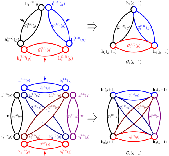
Figure 1: Second construction means for the simiplical networks for two special cases of $q=1$ and $q=2$. For each $k\in\{1,2,\ldots,q+2$}, the $q+1$ hub nodes $h_{k}^{(1,k)}(g-1)$, $h_{k}^{(2,k)}(g-1)$, $\ldots$, $h_{k}^{(k-1,k)}(g-1)$, $h_{k}^{(k,k+1)}(g-1)$, $\ldots$, $h_{k}^{(k,q+2)}(g-1)$ in the corresponding $q+1$ replicas of $\mathcal{G}_{q}(g-1)$ are identified as the hub node $h_{k}(g)$ of $\mathcal{G}_{q}(g)$.

The simplicial networks display some remarkable properties [24] as observed in most real networks [1]. They are scale-free, since their node degrees obey a power-law distribution $P(d)\sim d^{-\gamma_{q}}$ with $\gamma_{q}=2+\frac{\ln(q+2)}{\ln(q+1)}-\frac{\ln 2}{\ln(q+1)}$. They are small-world, since their diameters grow logarithmically with the number of nodes and their mean clustering coefficients approach a large constant $\frac{q^{2}+3q+3}{q^{2}+3q+5}$. Moreover, they have a finite spectral dimension $\frac{2[\ln(q^{2}+3q+3)-\ln 2]}{\ln(q+1)}$.

After introducing the two construction methods of the simplicial networks $\mathcal{G}_{q}(g)$ and their relevant properties, in the sequel, we will study analytically some combinatorial properties of the networks.

3 INDEPENDENCE NUMBER

For a simple connected graph $\mathcal{G}=(\mathcal{V}(\mathcal{G}),\mathcal{E}(\mathcal{G}))$, abbreviated as $\mathcal{G}=(\mathcal{V},\mathcal{E})$, an independent set of $\mathcal{G}$ is a proper subset $\mathcal{I}$ of $\mathcal{V}$ satisfying that each pair of nodes in $\mathcal{I}$ is not adjacent. An independent set is called a maximal independent set if it is not a subset of any other independent set. A maximal independent set is called a maximum independent set if it has the largest possible cardinality or size. The cardinality of any maximum independent set for a graph $\mathcal{G}$ is called the independence number of $\mathcal{G}$ and is denoted by $\alpha(\mathcal{G})$. We now study the independence number of graph $\mathcal{G}_{q}(g)$, denoted by $\alpha_{q}(g)$.

Theorem 3.1.

For all $g\geq 0$, the independence number of $\mathcal{G}_{q}(g)$ is:

$$\alpha_{q}(g)={\left[\frac{(q+1)(q+2)}{2}\right]}^{g}.$$ (6)

Proof 3.2.

For $g=0$, $\mathcal{G}_{q}(0)$ is a complete graph of $q+2$ nodes. It is obvious that $\alpha_{q}(0)=1$, which is consistent with Eq. (6).

For $g\geq 1$, by Definition 2.1, $\mathcal{G}_{q}(g)$ is obtained from $\mathcal{G}_{q}(g-1)$ through replacing each of $M_{g-1,q}$ edges in $\mathcal{G}_{q}(g-1)$ by a $(q+2)$-node complete graph, which includes the edge and its two end nodes. Let $\mathcal{K}_{q+2}^{(1)}$, $\mathcal{K}_{q+2}^{(2)}$, $\ldots$, $\mathcal{K}_{q+2}^{(M_{g-1,q})}$ denote the $M_{g-1,q}$ complete graphs, respectively, corresponding to the $M_{g-1,q}$ edges in graph $\mathcal{G}_{q}(g-1)$. Then, for any independent set $\mathcal{I}$ of $\mathcal{G}_{q}(g)$, there is at most one node in $\mathcal{K}_{q+2}^{(i)}$, $i=1,2,\ldots,M_{g-1,q}$. In other words, $\left|\mathcal{I}\cap\mathcal{K}_{q+2}^{(i)}\right|\leq 1$ for $i=1,2,\ldots,M_{g-1,q}$. Therefore, $|\mathcal{I}|\leq M_{g-1,q}={\left[\frac{(q+1)(q+2)}{2}\right]}^{g}$, implying $\alpha_{q}(g)\leq{\left[\frac{(q+1)(q+2)}{2}\right]}^{g}$.

On the other hand, for every node $u$ in $\mathcal{G}_{q}(g)$, which is created at generation $g$, it belongs to a certain clique $\mathcal{K}_{q+2}^{(i)}$ (namely, $u\in\mathcal{K}_{q+2}^{(i)}$), $1\leq i\leq M_{g-1,q}$, and is only connected to the other $q+1$ nodes in this $(q+2)$-clique. Therefore, by arbitrarily selecting one newly created node from each $\mathcal{K}_{q+2}^{(i)}$, $i=1,2,\ldots,M_{g-1,q}$, one obtains an independent set for $\mathcal{G}_{q}(g)$ with size equal to $M_{g-1,q}={\left[\frac{(q+1)(q+2)}{2}\right]}^{g}$, which leads to $\alpha_{q}(g)\geq{\left[\frac{(q+1)(q+2)}{2}\right]}^{g}$.

Combining the above arguments leads to the statement.

Equation (6) generalizes the result in [41] for $q=1$ to positive integer $q$.

4 DOMINATION NUMBER

For a graph $\mathcal{G}=(\mathcal{V},\mathcal{E})$, a dominating set for $\mathcal{G}$ is a subset $\mathcal{D}$ of $\mathcal{V}$ such that every node not in $\mathcal{D}$ is adjacent to at least one node in $\mathcal{D}$. A dominating set is called a minimal dominating set if it is not a proper subset of any other dominating set. A dominating set is called a minimum dominating set if it has the smallest cardinality among all dominating sets. The cardinality of any minimum dominating set for graph $\mathcal{G}$ is called the domination number of $\mathcal{G}$, denoted by $\gamma(\mathcal{G})$. For graph $\mathcal{G}$, the relation $\gamma(\mathcal{G})\leq\alpha(\mathcal{G})$ always holds [54, 55].

Let $\gamma_{q}(g)$ denote the domination number of graph $\mathcal{G}_{q}(g)$. When $g$ is small, $\gamma_{q}(g)$ is easily determined. Since $\mathcal{G}_{q}(0)$ is a complete graph of $q+2$ nodes, $\gamma_{q}(0)=1$, and every node can be considered as a minimum dominating set for $\mathcal{G}_{q}(0)$. For $\mathcal{G}_{q}(1)$, the domination number is obtained in the following lemma.

Lemma 4.1.

The domination number of graph $\mathcal{G}_{q}(1)$ is $\gamma_{q}(1)=q+1$. And each subset of the hub node set $\mathcal{V}_{\rm h}(\mathcal{G}_{q}(1))$ containing $q+1$ nodes is a minimum dominating set for $\mathcal{G}_{q}(1)$.

Proof 4.2.

By Proposition 2.2, $\mathcal{G}_{q}(1)$ can be generated by joining $\frac{(q+1)(q+2)}{2}$ copies of $\mathcal{K}_{q+2}$ at the $q+2$ hub nodes, which are denoted by $\mathcal{K}^{(i,j)}_{q+2}$, $1\leq i<j\leq q+2$. Now we show that for any dominating set $\mathcal{D}$ of $\mathcal{G}_{q}(1)$, we can construct a dominating set $\mathcal{D}^{\prime}$ including only hub nodes in $\mathcal{G}_{q}(1)$.

Suppose that $v\in\mathcal{D}$ is not a hub node. By construction, the neighbors of $v$ are all from a single complete graph $\mathcal{K}^{(i,j)}_{q+2}$. We can replace $v$ by hub node $h_{i}(1)$ or $h_{j}(1)$ to obtain a dominating set $\mathcal{D}_{v}$. In a similar way, we can replace other non-hub nodes in $\mathcal{D}_{v}$ to obtain a dominating set $\mathcal{D}^{\prime}$. Thus, to find the domination number for $\mathcal{G}_{q}(1)$, one can only choose hub nodes to form a minimum dominating set.

We continue to show that for any minimum dominating set $\mathcal{D}$ of $\mathcal{G}_{q}(1)$ containing only hub nodes, $|\mathcal{D}|=q+1$. By contradiction, assume that $|\mathcal{D}|<q+1$, which means that there exist at least two hub nodes $h_{i}(1)$ and $h_{j}(1)$ not in $\mathcal{D}$, which belong to the complete graph $\mathcal{K}^{(i,j)}_{q+2}$. Then, the non-hub nodes in $\mathcal{K}^{(i,j)}_{q+2}$ are not dominated, implying the $\mathcal{D}$ is not a dominating set. Therefore, $|\mathcal{D}|\geq q+1$ and $\gamma_{q}(1)\geq q+1$. On the other hand, it is easy to check that any $q+1$ hub nodes can dominate all nodes in $\mathcal{G}_{q}(1)$. Hence, $\gamma_{q}(1)=q+1$.

Figure 4.2 illustrates the minimum dominating sets of $\mathcal{G}_{1}(1)$ and $\mathcal{G}_{2}(1)$.

Examples of the minimum dominating sets for $\mathcal{G}_{1}(1)$ and $\mathcal{G}_{2}(1)$.

For a subset $\mathcal{C}$ of $\mathcal{V}(\mathcal{G}_{q}(g))$, if a node $v$ in $\mathcal{V}(\mathcal{G}_{q}(g))\backslash\mathcal{C}$ is adjacent to at least one node in $\mathcal{C}$, we say that $v$ is dominated by $\mathcal{C}$. Thus, if all nodes in $\mathcal{V}(\mathcal{G}_{q}(g))\backslash\mathcal{C}$ are dominated by $\mathcal{C}$, then $\mathcal{C}$ is a dominating set of $\mathcal{G}_{q}(g)$.

Lemma 4.3.

For a subset $\mathcal{C}$ of $\mathcal{V}(\mathcal{G}_{q}(g))$ corresponding to graph $\mathcal{G}_{q}(g)$ with $g\geq 1$, if all the non-hub nodes of $\mathcal{G}_{q}(g)$ are in $\mathcal{C}$ or dominated by $\mathcal{C}$, then $\mathcal{C}$ is a dominating set of $\mathcal{G}_{q}(g)$.

Proof 4.4.

We only need to prove that all the $q+2$ hub nodes of $\mathcal{G}_{q}(g)$ are either dominated by $\mathcal{C}$ or included in $\mathcal{C}$. For any hub node $h_{i}(g)$ ($i=1,2,\ldots,q+2$) of graph $\mathcal{G}_{q}(g)$, it and another hub node $h_{j}(g)$ ($i\neq j$) create a clique $\mathcal{K}_{q}$ with $q$ nodes at generation $g$, which, together with $h_{i}(g)$ and $h_{j}(g)$, form a $(q+2)$-clique in $\mathcal{G}_{q}(g)$. If $h_{i}(g)\in\mathcal{C}$, the lemma holds. For the case that $h_{i}(g)\notin\mathcal{C}$, we show below that $h_{i}(g)$ is dominated by a node in $\mathcal{C}$. Since the $q$ newly introduced nodes in $\mathcal{K}_{q}$ are non-hub nodes in $\mathcal{G}_{q}(g)$, for any node $v\in\mathcal{K}_{q}$, it is either included in $\mathcal{C}$ or dominated by $\mathcal{C}$. If $v\in\mathcal{C}$, then $h_{i}(g)$ is dominated by $\mathcal{C}$. If $v$ is not in $\mathcal{C}$ but dominated by $h_{j}(g)$ or other non-hub nodes in its generating $(q+2)$-clique, then $h_{i}(g)$ is dominated by $\mathcal{C}$.

We are now in position to determine the domination number $\gamma_{q}(g)$ of graph $\mathcal{G}_{q}(g)$ for the case of $g\geq 1$.

Theorem 4.5.

For all $g\geq 1$, the domination number of $\mathcal{G}_{q}(g)$ is:

$$\gamma_{q}(g)=\frac{q^{2}+2q-1}{q+3}{\left[\frac{(q+1)(q+2)}{2}\right]}^{g-1}+\frac{2(q+2)}{q+3}.$$

Proof 4.6.

From Proposition 2.2, $\mathcal{G}_{q}(g+1)$ can be generated by joining $\frac{(q+1)(q+2)}{2}$ copies of $\mathcal{G}_{q}(g)$ at the $q+2$ hub nodes, denoted by $\mathcal{G}_{q}^{(1)}(g)$, $\mathcal{G}_{q}^{(2)}(g)$, $\ldots$, $\mathcal{G}_{q}^{(\frac{(q+1)(q+2)}{2})}(g)$, respectively. Let $\mathcal{D}(\mathcal{G}_{q}(g+1))$ represent a dominating set of $\mathcal{G}_{q}(g+1)$. For any $i=1,2,\ldots,\frac{(q+1)(q+2)}{2}$, the non-hub nodes of $\mathcal{G}_{q}^{(i)}(g)$ are dominated or belong to $\mathcal{D}(\mathcal{G}_{q}(g+1))\cap\mathcal{G}_{q}^{(i)}(g)$. By Lemma 4.3, $\mathcal{D}(\mathcal{G}_{q}(g+1))\cap\mathcal{G}_{q}^{(i)}(g)$ is a dominating set of $\mathcal{G}_{q}^{(i)}(g)$. Then, $|\mathcal{D}(\mathcal{G}_{q}(g+1))|$ can be computed in terms of $|\mathcal{D}(\mathcal{G}_{q}(g+1))\cap\mathcal{G}_{q}^{(i)}(g)|$ as

$$|\mathcal{D}(\mathcal{G}_{q}(g+1))| =-q|\mathcal{D}(\mathcal{G}_{q}(g+1))\cap\mathcal{V}_{\rm h}(\mathcal{G}_{q}(g+1))|+$$

$$\quad\sum_{i=1}^{\frac{(q+1)(q+2)}{2}}|\mathcal{D}(\mathcal{G}_{q}(g+1))\cap\mathcal{G}_{q}^{(i)}(g)|,$$

where the first term on the right-hand side compensates for the overcounting of the hub nodes chosen in $\mathcal{D}(\mathcal{G}_{q}(g+1))$. Since $|\mathcal{V}_{\rm h}(\mathcal{G}_{q}(g+1))|=q+2$,

$$|\mathcal{D}(\mathcal{G}_{q}(g+1))|\geq \sum_{i=1}^{\frac{(q+1)(q+2)}{2}}|\mathcal{D}(\mathcal{G}_{q}(g+1))\cap\mathcal{G}_{q}^{(i)}(g)|$$

$$-q(q+2).$$

Particularly, when $\mathcal{D}(\mathcal{G}_{q}(g+1))$ is a minimum dominating set of $\mathcal{G}_{q}(g+1)$, denoted by $\mathcal{D}_{\rm min}(\mathcal{G}_{q}(g+1))$,

$$\quad|\mathcal{D}_{\rm min}(\mathcal{G}_{q}(g+1))|$$

$$\geq-q(q+2)+\sum_{i=1}^{\frac{(q+1)(q+2)}{2}}|\mathcal{D}_{\rm min}(\mathcal{G}_{q}(g+1))\cap\mathcal{G}_{q}^{(i)}(g)|$$

$$\geq-q(q+2)+\frac{(q+1)(q+2)}{2}|\mathcal{D}_{\rm min}(\mathcal{G}_{q}(g))|,$$ (7)

where the second inequality is due to the fact that $\mathcal{D}_{\rm min}(\mathcal{G}_{q}(g+1))\cap\mathcal{G}_{q}^{(i)}(g)$ is a dominating set of $\mathcal{G}_{q}^{(i)}(g)$, with cardinality larger than that of a minimum dominating set for $\mathcal{G}_{q}^{(i)}(g)$.

Note that the terms on both sides of Eq. (7) are equal to each other, when all hub nodes of $\mathcal{G}_{q}(g+1)$ are in $\mathcal{D}_{\rm min}(\mathcal{G}_{q}(g+1))$ and the intersection of $\mathcal{D}_{\rm min}(\mathcal{G}_{q}(g+1))$ with each $\mathcal{G}_{q}^{(i)}(g)$ forms a minimum dominating set of $\mathcal{G}_{q}^{(i)}(g)$. In other words, $\mathcal{D}_{\rm min}(\mathcal{G}_{q}(g+1))$ is the union of the minimum dominating sets $\mathcal{D}^{(i)}_{\rm min}(\mathcal{G}_{q}(g))$ of $\mathcal{G}_{q}^{(i)}(g)$, such that $\mathcal{D}_{\rm min}(\mathcal{G}_{q}(g+1))$ includes all hub nodes of $\mathcal{G}_{q}(g+1)$. Thus, for each $\mathcal{D}^{(i)}_{\rm min}(\mathcal{G}_{q}(g))$, it contains as many hub nodes in $\mathcal{G}_{q}^{(i)}(g)$ as possible. For $g=1$, all hub nodes of $\mathcal{G}_{q}(2)$ and arbitrary other $q-1$ hub nodes for each $\mathcal{G}_{q}^{(i)}(1)$ constitute a minimum dominating set $\mathcal{D}_{\rm min}(\mathcal{G}_{q}(2))$ of $\mathcal{G}_{q}(2)$. By Lemma 4.3, $\mathcal{D}_{\rm min}(\mathcal{G}_{q}(2))\cap\mathcal{G}_{q}^{(i)}(1)$ forms a minimum dominating set of $\mathcal{G}_{q}^{(i)}(1)$. It is easy to verify that for $g=1$, the terms on both sides of Eq. (7) are equal to each other. Using $\mathcal{D}_{\rm min}(\mathcal{G}_{q}(2))$, we can construct a minimum dominating set $\mathcal{D}_{\rm min}(\mathcal{G}_{q}(3))$ of $\mathcal{G}_{q}(3)$ by merging the minimum dominating sets $\mathcal{D}^{(i)}_{\rm min}(\mathcal{G}_{q}(2))$ for each $\mathcal{G}_{q}^{(i)}(2)$ and removing those duplicate hub nodes of $\mathcal{G}_{q}(3)$. In a similar way, we can iteratively construct a minimum dominating set $\mathcal{D}_{\rm min}(\mathcal{G}_{q}(g))$ for $\mathcal{G}_{q}(g)$ when $g\geq 4$, for which the equal mark holds for Eq. (7). Then, we have

$$\gamma_{q}(g+1)=-q(q+2)+\frac{(q+1)(q+2)}{2}\gamma_{q}(g)$$ (8)

for all $g\geq 1$. With initial condition $\gamma_{q}(1)=q+1$, the above equation is solved to obtain:

$$\gamma_{q}(g)=\frac{q^{2}+2q-1}{q+3}{\left[\frac{(q+1)(q+2)}{2}\right]}^{g-1}+\frac{2(q+2)}{q+3}.$$

This finishes the proof.

Theorem 4.5 is reduced to the result in [40] obtained for $q=1$.

5 CHROMATIC NUMBER

Node coloring of a graph $\mathcal{G}=(\mathcal{V},\mathcal{E})$ is a way of coloring the nodes of $\mathcal{G}$ such that no two adjacent nodes in $\mathcal{V}$ are of the same color. The chromatic number of a graph $\mathcal{G}$, denoted by $\chi(\mathcal{G})$, is the smallest number of colors needed to color the nodes of $\mathcal{G}$. For graph $\mathcal{G}$, node coloring is closely related to its chromatic polynomial $P(\mathcal{G},\lambda)$, which is a polynomial counting the number of distinct ways to color $\mathcal{G}$ with $\lambda$ or fewer colors. The chromatic polynomial was first introduced by George David Birkhoff [56]. It contains at least as much information about the colorability of graph $\mathcal{G}$ as does the chromatic number. Indeed, $\chi(\mathcal{G})$ is the smallest positive integer that is not a root of the chromatic polynomial, that is,

$$\chi(\mathcal{G})={\rm min}\{\lambda:\,P(\mathcal{G},\lambda)>0\}.$$ (9)

The chromatic polynomial for the $q$-node complete graph $\mathcal{K}_{q}$ is

$$P(\mathcal{K}_{q},\lambda)=\lambda(\lambda-1)(\lambda-2)\cdots(\lambda-q+1).$$ (10)

For two graphs $\mathcal{G}=(\mathcal{V}(\mathcal{G}),\mathcal{E}(\mathcal{G}))$ and $\mathcal{G^{\prime}}=(\mathcal{V}(\mathcal{G^{\prime}}),\mathcal{E}(\mathcal{G^{\prime}}))$, let $\mathcal{G}\cup\mathcal{G^{\prime}}$ represent their union with node set $\mathcal{V}(\mathcal{G})\cup\mathcal{V}(\mathcal{G^{\prime}})$ and edge set $\mathcal{E}(\mathcal{G})\cup\mathcal{E}(\mathcal{G^{\prime}})$, and let $\mathcal{G}\cap\mathcal{G^{\prime}}$ denote their intersection with node set $\mathcal{V}(\mathcal{G})\cap\mathcal{V}(\mathcal{G^{\prime}})$ and edge set $\mathcal{E}(\mathcal{G})\cap\mathcal{E}(\mathcal{G^{\prime}})$. Then, the chromatic polynomial of graph $\mathcal{G}\cup\mathcal{G^{\prime}}$ is [57]

$$P(\mathcal{G}\cup\mathcal{G^{\prime}},\lambda)=\frac{P(\mathcal{G},\lambda)\cdot P(\mathcal{G^{\prime}},\lambda)}{P(\mathcal{G}\cap\mathcal{G^{\prime}},\lambda)}\,.$$ (11)

Lemma 5.1.

For all $g\geq 0$, the chromatic polynomial of $\mathcal{G}_{q}(g)$ is

$$P(\mathcal{G}_{q}(g),\lambda)$$

$$=\lambda(\lambda-1)\prod_{i=2}^{q+1}{(\lambda-i)}^{\frac{2}{q(q+3)}{\left[\frac{(q+1)(q+2)}{2}\right]}^{g+1}-\frac{2}{q(q+3)}}.$$ (12)

Proof 5.2.

Proposition 2.2 shows that $\mathcal{G}_{q}(g+1)$ is in fact an amalgamation of $\frac{(q+1)(q+2)}{2}$ copies of $\mathcal{G}_{q}(g)$ at the $q+2$ hub nodes, denoted by $\mathcal{G}_{q}^{(1)}(g)$, $\mathcal{G}_{q}^{(2)}(g)$, $\ldots$, $\mathcal{G}_{q}^{(\frac{(q+1)(q+2)}{2})}(g)$, respectively. Since the hub nodes of $\mathcal{G}_{q}(g+1)$ are linked to each other, $\mathcal{G}_{q}(g+1)$ can be also obtained from the $\frac{(q+1)(q+2)}{2}$ copies of $\mathcal{G}_{q}(g)$ by merging them at the $\frac{(q+1)(q+2)}{2}$ edges of the complete graph $\mathcal{K}_{q+2}$ formed by their $q+2$ hub nodes. That is,

$$\mathcal{G}_{q}(g+1)=\mathcal{K}_{q+2}\cup\mathcal{G}_{q}^{(1)}(g)\cup\mathcal{G}_{q}^{(2)}(g)\cup\ldots\cup\mathcal{G}_{q}^{\frac{(q+1)(q+2)}{2}}(g),$$

where

$$\mathcal{K}_{q+2}\cap\mathcal{G}_{q}^{(1)}(g)=\mathcal{K}_{2}$$

and

$$\bigg{(}\mathcal{K}_{q+2}\cup\mathcal{G}_{q}^{(1)}(g)\cup\mathcal{G}_{q}^{(2)}(g)\ldots\cup\mathcal{G}_{q}^{(j)}(g)\bigg{)}\cap\mathcal{G}_{q}^{(j+1)}(g)=\mathcal{K}_{2},$$

for all $1\leq j<\frac{(q+1)(q+2)}{2}$. Thus, by using Eq. (11) $\frac{(q+1)(q+2)}{2}$ times, we establish a recursion relation between $P(\mathcal{G}_{q}(g+1),\lambda)$ and $P(\mathcal{G}_{q}(g),\lambda)$ as

$$P(\mathcal{G}_{q}(g+1),\lambda)=\frac{{\left(P(\mathcal{G}_{q}(g),\lambda)\right)}^{\frac{(q+1)(q+2)}{2}}\cdot P(\mathcal{K}_{q+2},\lambda)}{{\left(P(\mathcal{K}_{2},\lambda)\right)}^{\frac{(q+1)(q+2)}{2}}}.$$ (13)

With the initial condition $P(\mathcal{G}_{q}(0),\lambda)=P(\mathcal{K}_{q+2},\lambda)$ and Eq. (10), Eq. (13) is solved to obtain Eq. (5.1).

Combining Eq. (9) and Lemma 5.1, one obtains the following theorem.

Theorem 5.3.

For all $g\geq 0$, the chromatic number of $\mathcal{G}_{q}(g)$ is $\chi(\mathcal{G}_{q}(g))=q+2$.

6 ENUMERATION OF ACYCLIC ORIENTATIONS

For an undirected graph $\mathcal{G}=(\mathcal{V},\mathcal{E})$, an acyclic orientation of $\mathcal{G}$ is to assign a direction to each edge in $\mathcal{G}$ to make it into a directed acyclic graph [58]. An acyclic orientation of $\mathcal{G}$ is called an acyclic root-connected orientation when there exists a distinct root node reachable from every node in $\mathcal{G}$ in the resulting directed graph [59].

This section is devoted to the determination of the number of acyclic orientations, as well as the number of acyclic root-connected orientations in graph $\mathcal{G}_{q}(g)$. To achieves this goal, we resort to the tool of Tutte polynomial [60]. For graph $\mathcal{G}=(\mathcal{V}(\mathcal{G}),\mathcal{E}(\mathcal{G}))$, its Tutte polynomial $T(\mathcal{G};x,y)$ is defined as

$$T(\mathcal{G};x,y)=\sum_{\mathcal{H}\subseteq\mathcal{G}}{(x-1)}^{r(\mathcal{G})-r(\mathcal{H})}{(y-1)}^{n(\mathcal{H})},$$ (14)

where the sum runs over all the spanning subgraphs $\mathcal{H}$ of $\mathcal{G}$, $r(\mathcal{G})=|\mathcal{V}(\mathcal{G})|-k(\mathcal{G})$ is the rank of $\mathcal{G}$, $n(\mathcal{G})=|\mathcal{E}(\mathcal{G})|-|\mathcal{V}(\mathcal{G})|+k(\mathcal{G})$ is the nullity of $\mathcal{G}$, and $k(\mathcal{G})$ is the number of components of $\mathcal{G}$.

The evaluation of the Tutte polynomial of graph $\mathcal{G}$ at a particular point on $(x,y)$-plane is related to many combinatorial aspects of $\mathcal{G}$ [61]. It has been shown that $T(\mathcal{G};2,0)$ equals the number of acyclic orientations of $\mathcal{G}$ [58], while $T(\mathcal{G};1,0)$ is equivalent to the number of root-connected acyclic orientations of $\mathcal{G}$ [59]. Moreover, the Tutte polynomial $T(\mathcal{G};x,y)$ is also relevant to the chromatic polynomial $P(\mathcal{G},\lambda)$ of graph $\mathcal{G}$. Specifically, $P(\mathcal{G},\lambda)$ can be represented in terms of $T(\mathcal{G};x,y)$ at $y=0$ as

$$P(\mathcal{G},\lambda)={(-\lambda)}^{k(\mathcal{G})}{(-1)}^{n(\mathcal{G})}T(\mathcal{G};1-\lambda,0).$$ (15)

This connection between the Tutte polynomial and the chromatic polynomial allows to determine the number of acyclic orientations and root-connected acyclic orientations for $\mathcal{G}_{q}(g)$.

Theorem 6.1.

For graph $\mathcal{G}_{q}(g)$ with $g\geq 0$, the number of acyclic orientations is

$$N_{\rm ao}(\mathcal{G}_{q}(g))=2{\left[\frac{(q+2)!}{2}\right]}^{\frac{2}{q(q+3)}{\left[\frac{(q+1)(q+2)}{2}\right]}^{g+1}-\frac{2}{q(q+3)}},$$ (16)

and the number of root-connected acyclic orientations is

$$N_{\rm rao}(\mathcal{G}_{q}(g))={[(q+1)!]}^{\frac{2}{q(q+3)}{\left[\frac{(q+1)(q+2)}{2}\right]}^{g+1}-\frac{2}{q(q+3)}}.$$ (17)

Proof 6.2.

Lemma 5.1 gives the chromatic polynomial for graph $\mathcal{G}_{q}(g)$, which together with Eq. (15) governing the Tutte polynomial and the chromatic polynomial yields

$$T(\mathcal{G}_{q}(g);x,0)=x\prod_{i=1}^{q}{(x+i)}^{\frac{2}{q(q+3)}{\left[\frac{(q+1)(q+2)}{2}\right]}^{g+1}-\frac{2}{q(q+3)}}.$$ (18)

By replacing $x=2$ and $x=1$ in Eq. (18), we obtain the number of acyclic orientations and the number of acyclic root-connected orientations of $\mathcal{G}_{q}(g)$, as given by Eqs. (16) and (17), respectively.

7 NUMBER OF PERFECT MATCHINGS

For a graph $\mathcal{G}=(\mathcal{V},\mathcal{E})$, a matching $\mathcal{M}$ of $\mathcal{G}$ is a subset of $\mathcal{E}$ such that no two edges in $\mathcal{M}$ share a common node. A node is called matched or covered by a matching, if it is an endpoint of one of the edges in the matching. For a graph $\mathcal{G}$ with even number of nodes, a perfect matching of $\mathcal{G}$ is a matching which matches all nodes in the graph. It was shown that for a complete graph with even $q$ nodes, the number of its perfect matchings is $(q-1)!!$ [62].

For graph $\mathcal{G}_{q}(g+1)$ and $\mathcal{G}_{q}(g)$, by the second construction approach given in Proposition 2.2, the number of their nodes satisfies $N_{g+1,q}=\frac{(q+1)(q+2)}{2}N_{g,q}-q(q+2)$. Hence, $N_{g,q}$ is always even when $q$ is an even number; but $N_{g,q}$ may be an odd number when $q$ is odd. Then, for odd $q$, a perfect matching may not exist for $\mathcal{G}_{q}(g)$. Below, we will show that for an even $q$, perfect matchings always exist in $\mathcal{G}_{q}(g)$.

Theorem 7.1.

When $q$ is even and not less than 2, perfect matchings always exist in $\mathcal{G}_{q}(g)$ for all $g\geq 0$.

Proof 7.2.

By induction on $g$. For $g=0$, $\mathcal{G}_{q}(0)$ is a complete graph with $q+2$ nodes. There exist $(q+1)!!$ perfect matchings in $\mathcal{G}_{q}(0)$. Thus, the result is true for $g=0$. Suppose that there is a perfect matchings in $\mathcal{G}_{q}(g)$. Let $\mathcal{M}_{g}$ be a perfect matching of $\mathcal{G}_{q}(g)$ for $g\geq 0$. By construction in Definition 2.1, $\mathcal{G}_{q}(g+1)$ is obtained from $\mathcal{G}_{q}(g)$ by replacing each of $M_{g,q}$ edges in $\mathcal{G}_{q}(g)$ by a complete graph having $(q+2)$ nodes, which includes the edge and its two end nodes. Let $\mathcal{K}_{q+2}^{(1)}$, $\mathcal{K}_{q+2}^{(2)}$, $\ldots$, $\mathcal{K}_{q+2}^{(M_{g,q})}$ denote the $M_{g,q}$ complete graphs. For each of these complete graphs, corresponding to an edge in $\mathcal{G}_{q}(g)$, since the two end nodes are covered by $\mathcal{M}_{g}$, one can chose $q/2$ independent edges in the complete graph to cover the remaining nodes. In this way, one obtains a perfect matchings for $\mathcal{G}_{q}(g+1)$.

We proceed to determine the number of perfect matchings in $\mathcal{G}_{q}(g)$ for even $q$, denoted by $N_{\rm per}(g,q)$. For this purpose, we first define some intermediary variables for graph $\mathcal{G}_{q}(g)$. Let $\Upsilon_{0}(\mathcal{G}_{q}(g))$ denote the set of matchings of $\mathcal{G}_{q}(g)$ such that the two hub nodes $h_{1}(g)$ and $h_{2}(g)$ are vacant, while all the other nodes in $\mathcal{G}_{q}(g)$ are matched. Let $A_{q}(g)$ be the cardinality of $\Upsilon_{0}(\mathcal{G}_{q}(g))$. Let $\Upsilon_{1}(\mathcal{G}_{q}(g))$ be the set of perfect matchings of $\mathcal{G}_{q}(g)$, and let $B_{q}(g)=N_{\rm per}(g,q)$ be the cardinality of $\Upsilon_{1}(\mathcal{G}_{q}(g))$. Note that in $\mathcal{G}_{q}(g)$, there does not exist such a match that either $h_{1}(g)$ or $h_{2}(g)$ is vacant, while all other nodes are covered.

Theorem 7.3.

For even $q\geq 2$ and $g\geq 0$, the number of perfect matchings in $\mathcal{G}_{q}(g)$ is

$$N_{\rm per}(g,q)={[(q+1)!!]}^{\frac{2}{q(q+3)}{\left[\frac{(q+1)(q+2)}{2}\right]}^{g+1}-\frac{2}{q(q+3)}}\times$$

$$\quad{(q+1)}^{-\frac{2(q+2)}{q{(q+3)}^{2}}{\left[\frac{(q+1)(q+2)}{2}\right]}^{g+1}+\frac{q+2}{q+3}g+\frac{(q+1){(q+2)}^{2}}{q{(q+3)}^{2}}}.$$ (19)

Proof 7.4.

Note that $B_{q}(g)=N_{\rm per}(g,q)$. We now derive recursive relations for $A_{q}(g+1)$ and $B_{q}(g+1)$, on the basis of which we further determine an exact expression for $B_{q}(g)$. From Proposition 2.2 and the definitions of $A_{q}(g)$ and $B_{q}(g)$, one obtains the following recursion relations for $A_{q}(g)$ and $B_{q}(g)$:

$$A_{q}(g+1)=(q-1)!!B_{q}^{\frac{q}{2}}(g)A_{q}^{\frac{q^{2}+2q+2}{2}}(g)\,,$$ (20)

$$B_{q}(g+1)=(q+1)!!B_{q}^{\frac{q}{2}+1}(g)A_{q}^{\frac{q(q+2)}{2}}(g)\,.$$ (21)

Equation (20) is explained as follows. By Proposition 2.2, any matching for graph $\mathcal{G}_{q}(g+1)$ can be constructed by joining the matchings of the $\frac{(q+1)(q+2)}{2}$ copies of $\mathcal{G}_{q}(g)$ at the $q+2$ hub vertices. According to the aforementioned analysis, for any matching of $\mathcal{G}_{q}(g+1)$, the matched hub vertices of $\mathcal{G}_{q}(g+1)$ must come in pairs. Then, any matching in $\Upsilon_{0}(\mathcal{G}_{q}(g+1))$ can be obtained recursively from those in $\Upsilon_{0}(\mathcal{G}_{q}(g))$ and $\Upsilon_{1}(\mathcal{G}_{q}(g))$ for the $\frac{(q+1)(q+2)}{2}$ copies of $\mathcal{G}_{q}(g)$, denoted by $\mathcal{G}_{q}^{(i)}(g)$, $i=1,2,\ldots,\frac{(q+1)(q+2)}{2}$. Moreover, related quantities in Eq. (20) are accounted for as follows: $(q-1)!!$ indicates the ways of pairing the $q$ matched hub vertices, which is equal to the number of perfect matchings of $\mathcal{K}_{q}$; $\frac{q}{2}$ denotes the pairs of matched hub vertices $h_{1}(g)$ or $h_{2}(g)$ in $\mathcal{G}_{q}^{(i)}(g)$; while $\frac{q^{2}+2q+2}{2}=\frac{(q+1)(q+2)}{2}-\frac{q}{2}$ represents the cases that $h_{1}(g)$ or $h_{2}(g)$ are vacant in $\mathcal{G}_{q}^{(i)}(g)$. Analogously, we can interpret Eq. (21).

Figure 7.4 gives a graphic illustration of Eqs. (20) and (21) for a particular case of $q=2$.

Dividing Eq. (21) by Eq. (20) yields a recursive relation for $\frac{B_{q}(g)}{A_{q}(g)}$ as

$$\frac{B_{q}(g+1)}{A_{q}(g+1)}=(q+1)\frac{B_{q}(g)}{A_{q}(g)}\,.$$ (22)

With the initial condition $\frac{B_{q}(0)}{A_{q}(0)}=\frac{(q+1)!!}{(q-1)!!}=q+1$, Eq. (22) is solved to obtain

$$\frac{B_{q}(g)}{A_{q}(g)}={(q+1)}^{g+1},$$ (23)

which implies

$$A_{q}(g)=\frac{B_{q}(g)}{{(q+1)}^{g+1}}.$$ (24)

Plugging this expression into Eq. (21) leads to

$$B_{q}(g+1)=\frac{(q+1)!!}{{(q+1)}^{\frac{q(q+2)(g+1)}{2}}}B_{q}^{\frac{(q+1)(q+2)}{2}}(g)\,.$$ (25)

Under the initial condition $B_{q}(0)=(q+1)!!$, Eq. (25) is solved to obtain Eq. (7.3).

Illustration of recursive configurations for matchings in $\Upsilon_{0}(\mathcal{G}_{q}(g+1))$ and $\Upsilon_{1}(\mathcal{G}_{q}(g+1))$ for graph $\mathcal{G}_{q}(g+1)$ with $q=2$. Each filled node represents a covered node, while each empty node represents a vacant node.

8 NUMBER OF SPANNING TREES

For a graph $\mathcal{G}=(\mathcal{V},\mathcal{E})$ with $|\mathcal{V}|$ nodes, a spanning tree of $\mathcal{G}$ is a connected subgraph of $\mathcal{G}$ that has a node set $\mathcal{V}$ and $|\mathcal{V}|-1$ edges. The number of spanning trees in a graph $\mathcal{G}$ is called the complexity of $\mathcal{G}$, which is an important graph invariant [63].

Lemma 8.1.

Let $u$ and $v$ denote two distinct nodes in a complete graph $\mathcal{K}_{q}$ with $q\geq 3$ nodes. Let $N_{u,v}(\mathcal{K}_{q})$ be the number of spanning forests for $\mathcal{K}_{q}$, each of which consists two trees such that $u$ and $v$ belong to the two different trees. Then, $N_{u,v}(\mathcal{K}_{q})=2q^{q-3}$.

Proof 8.2.

Obviously, $N_{u,v}(\mathcal{K}_{q})$ equals the number of those spanning trees in $\mathcal{K}_{q}$, in each of which $u$ and $v$ are adjacent to each. By Cayley’s formula [64], the number of spanning trees of a $q$-node complete graph is $q^{q-2}$. For a randomly chosen spanning tree $\mathcal{T}$ of $\mathcal{K}_{q}$, the expected degree of node $u$ is $\frac{2(q-1)}{q}$. Then, in $\mathcal{T}$ the probability that $u$ is a neighbor of $v$ is $\frac{2(q-1)}{q}\cdot\frac{1}{q-1}=\frac{2}{q}$. Therefore, $N_{u,v}(\mathcal{K}_{q})=q^{q-2}\cdot\frac{2}{q}=2q^{q-3}$.

Theorem 8.3.

Let $N_{\rm st}(g,q)$ be the number of spanning trees in graph $\mathcal{G}_{q}(g)$ with $g\geq 0$ and $q\geq 1$. Then,

$$N_{\rm st}(g,q)=2^{\frac{2(q+1)}{q{(q+3)}^{2}}{\left[\frac{(q+1)(q+2)}{2}\right]}^{g+1}-\left(\frac{q+1}{q+3}\right)g-\frac{{(q+1)}^{2}(q+2)}{{q(q+3)}^{2}}}\times$$

$$\quad{(q+2)}^{\frac{2(q^{2}+2q-1)}{q{(q+3)}^{2}}{\left[\frac{(q+1)(q+2)}{2}\right]}^{g+1}+\left(\frac{q+1}{q+3}\right)g+\frac{q^{3}+2q^{2}-q+2}{{q(q+3)}^{2}}}.$$

Proof 8.4.

By Definition 2.1, $\mathcal{G}_{q}(g+1)$ is obtained from $\mathcal{G}_{q}(g)$ through replacing every edge in $\mathcal{G}_{q}(g)$ by a $\mathcal{K}_{q+2}$ clique, which contains the edge and its two end nodes. Accordingly, for any spanning tree $\mathcal{T}_{g}$ for $\mathcal{G}_{q}(g)$, one can construct a spanning tree for $\mathcal{G}_{q}(g+1)$ in the following way: replace each edge in $\mathcal{T}_{g}$ by a spanning tree of the $\mathcal{K}_{q+2}$ clique and replace each edge $(u,v)$ in $\mathcal{G}_{q}(g)$ but absent in $\mathcal{T}_{g}$ by a spanning forest for $\mathcal{K}_{q+2}$, which consists two trees such that $u$ and $v$ are in different trees. Thus, using Lemma 8.1, one obtains

$$\quad N_{\rm st}(g+1,q)$$

$$=[(q+2)^{q}]^{N_{g,q}-1}\,[2(q+2)^{q-1}]^{M_{g,q}-N_{g,q}+1}\,N_{\rm st}(g,q)$$

$$=2^{M_{g,q}-N_{g,q}+1}\,{(q+2)}^{(q-1)M_{g,q}+N_{g,q}-1}\,N_{\rm st}(g,q),$$ (26)

where $N_{g,q}-1$ is the number of edges in the spanning tree $\mathcal{T}_{g}$ in $\mathcal{G}_{q}(g)$, and $M_{g,q}-N_{g,q}+1$ is the number of edges which exist in $\mathcal{G}_{q}(g)$ but is absent in $\mathcal{T}_{g}$, in other words, the number of edges in $\mathcal{G}_{q}(g)$ minus the number of edges in $\mathcal{T}_{g}$. Plugging the expressions for $N_{g,q}$ and $M_{g,q}$ in Eqs. (4) and (3) into Eq. (8.4) gives

$$\quad N_{\rm st}(g+1,q)$$

$$=N_{\rm st}(g,q)2^{\frac{q+1}{q+3}{\left[\frac{(q+1)(q+2)}{2}\right]}^{g+1}-\frac{q+1}{q+3}}$$

$$\quad¡¡\cdot{(q+2)}^{\frac{q^{2}+2q-1}{q+3}{\left[\frac{(q+1)(q+2)}{2}\right]}^{g+1}+\frac{q+1}{q+3}}.$$ (27)

With the initial condition $N_{\rm st}(0,q)={(q+2)}^{q}$, one obtains

$$N_{\rm st}(g,q)$$

$$= 2^{\frac{q+1}{q+3}\sum_{i=1}^{g}{\left[\frac{(q+1)(q+2)}{2}\right]}^{i}-\frac{q+1}{q+3}g}\times{(q+2)}^{q}\times$$

$${(q+2)}^{\frac{q^{2}+2q-1}{q+3}\sum_{i=1}^{g}{\left[\frac{(q+1)(q+2)}{2}\right]}^{i}+\frac{q+1}{q+3}g}$$

$$= 2^{\frac{2(q+1)}{q{(q+3)}^{2}}{\left[\frac{(q+1)(q+2)}{2}\right]}^{g+1}-\left(\frac{q+1}{q+3}\right)g-\frac{{(q+1)}^{2}(q+2)}{{q(q+3)}^{2}}}\times$$

$${(q+2)}^{\frac{2(q^{2}+2q-1)}{q{(q+3)}^{2}}{\left[\frac{(q+1)(q+2)}{2}\right]}^{g+1}+\left(\frac{q+1}{q+3}\right)g+\frac{q^{3}+2q^{2}-q+2}{{q(q+3)}^{2}}},$$

which completes the proof.

Note that Theorem 8.3 is consistent with result in [24], obtained using different technique, and reduces to the result [33] for the special case of $q=1$.

9 CONCLUSIONS

In this paper, we presented a systematic analytical study of combinatorial properties for a class of iteratively generating simplicial networks, based on their particular construction and self-similar structure. We derived the domination number, the independence number, and the chromatic number. Moreover, we obtained exact expressions for the number of spanning trees, the number of perfect matchings for even $q$, the number of acyclic orientations, and the number of root-connected acyclic orientations.

The considered combinatorial problems are a fundamental research subject of theoretical computer science, many of which are NP-hard and even #P-complete for a general graph. It is thus of great interest to study the special family of graphs for which these challenging combinatorial problems can be exactly solved. In addition, since the considered combinatorial problems are relevant to various practical application in the aspects of network science and graph data miming, this work provides insight into understanding the applications of these combinatorial problems for simplicial complexes.

Finally, it is worth mentioning that the studied simplicial networks are in fact constructed iteratively by edge corona product, which leads to the self-similarity of the resulting graphs. It is expected that our computation approach and process for relevant problems are also applicable to other graph families [65, 66, 67, 68, 69, 70, 71] with self-similar properties, built by other graph operations. We note that our techniques also have some limitations. For example, they do not apply to recursive graphs with stochasticity [72, 73].

References

- [1] M. E. Newman, The structure and function of complex networks, SIAM Rev. 45(2) (2003) 167–256.
- [2] A.-L. Barabási, Network science (Cambridge University Press, 2016).
- [3] A. R. Benson, D. F. Gleich and J. Leskovec, Higher-order organization of complex networks, Science 353(6295) (2016) 163–166.
- [4] J. Grilli, G. Barabás, M. J. Michalska-Smith and S. Allesina, Higher-order interactions stabilize dynamics in competitive network models, Nature 548(7666) (2017) p. 210.
- [5] A. R. Benson, R. Abebe, M. T. Schaub, A. Jadbabaie and J. Kleinberg, Simplicial closure and higher-order link prediction, Proc. Natl. Acad. Sci. 115(48) (2018) E11221–E11230.
- [6] V. Salnikov, D. Cassese and R. Lambiotte, Simplicial complexes and complex systems, Eur. J. Phys. 40(1) (2018) p. 014001.
- [7] I. Lacopini, G. Petri, A. Barrat and V. Latora, Simplicial models of social contagion, Nat. Commun. 10(1) (2019) p. 2485.
- [8] A. Patania, G. Petri and F. Vaccarino, The shape of collaborations, EPJ Data Sci. 6(1) (2017) p. 18.
- [9] C. Giusti, E. Pastalkova, C. Curto and V. Itskov, Clique topology reveals intrinsic geometric structure in neural correlations, Proc. Natl. Acad. Sci. U.S.A. 112(44) (2015) 13455–13460.
- [10] M. W. Reimann, M. Nolte, M. Scolamiero, K. Turner, R. Perin, G. Chindemi, P. Dłotko, R. Levi, K. Hess and H. Markram, Cliques of neurons bound into cavities provide a missing link between structure and function, Front. Comput. Neurosci. 11 (2017) p. 48.
- [11] S. Wuchty, Z. N. Oltvai and A.-L. Barabási, Evolutionary conservation of motif constituents in the yeast protein interaction network, Nat. Genet. 35(2) (2003) p. 176.
- [12] F. Battiston, G. Cencetti, I. Iacopini, V. Latora, M. Lucas, A. Patania, J.-G. Young and G. Petri, Networks beyond pairwise interactions: Structure and dynamics, Phys. Rep. 907 (2021) 1–68.
- [13] G. Bianconi and R. M. Ziff, Topological percolation on hyperbolic simplicial complexes, Phys. Rev. E 98(5) (2018) p. 052308.
- [14] U. Alvarez-Rodriguez, F. Battiston, G. F. de Arruda, Y. Moreno, M. Perc and V. Latora, Evolutionary dynamics of higher-order interactions in social networks, Nat. Hum. Behav. 5 (2021) 586–595.
- [15] P. S. Skardal and A. Arenas, Abrupt desynchronization and extensive multistability in globally coupled oscillator simplexes, Phys. Rev. Lett. 122(24) (2019) p. 248301.
- [16] L. Gambuzza, F. Di Patti, L. Gallo, S. Lepri, M. Romance, R. Criado, M. Frasca, V. Latora and S. Boccaletti, Stability of synchronization in simplicial complexes, Nat. Commun. 12(1) (2021) 1–13.
- [17] J. T. Matamalas, S. Gómez and A. Arenas, Abrupt phase transition of epidemic spreading in simplicial complexes, Phys. Rev. Research 2(1) (2020) p. 012049.
- [18] O. T. Courtney and G. Bianconi, Weighted growing simplicial complexes, Phys. Rev. E 95(6) (2017) p. 062301.
- [19] G. Petri and A. Barrat, Simplicial activity driven model, Phys. Rev. Lett. 121(22) (2018) p. 228301.
- [20] K. Kovalenko, I. Sendiña-Nadal, N. Khalil, A. Dainiak, D. Musatov, A. M. Raigorodskii, K. Alfaro-Bittner, B. Barzel and S. Boccaletti, Growing scale-free simplices, Commun. Phys. 4(1) (2021) 1–9.
- [21] A. Hatcher, Algebraic Topology (Cambridge University Press, 2002).
- [22] T. W. Haynes and L. M. Lawson, Applications of E-graphs in network design, Networks 23(5) (1993) 473–479.
- [23] T. W. Haynes and L. M. Lawson, Invariants of E-graphs, Int. J. Comput. Math. 55(1-2) (1995) 19–27.
- [24] Y. Wang, Y. Yi, W. Xu and Z. Zhang, Modeling higher-order interactions in complex networks by edge product of graphs, Comput. J. 65(9) (2022) 2347–2359.
- [25] M. Zhu, W. Xu, Z. Zhang, H. Kan and G. Chen, Resistance distances in simplicial networks, Comput. J. (in press) (2022).
- [26] S. N. Dorogovtsev, A. V. Goltsev and J. F. F. Mendes, Pseudofractal scale-free web, Phys. Rev. E 65(6) (2002) p. 066122.
- [27] X. Zhou and Z. Zhang, Edge domination number and the number of minimum edge dominating sets in pseudofractal scale-free web and sierpiński gasket, Fractals 29(07) (2021) p. 2150209.
- [28] C. Xing and H. Yuan, Lazy random walks on pseudofractal scale-free web with a perfect trap, Fractals 30(1) (2022) p. 2250030.
- [29] X. Wang, W. Slamu, K. Yu and Y. Zhu, Maximum matchings in a pseudofractal scale-free web, Fractals 30(4) (2022) p. 2250077.
- [30] H. D. Rozenfeld, S. Havlin and D. Ben-Avraham, Fractal and transfractal recursive scale-free nets, New J. Phys. 9(6) (2007) p. 175.
- [31] Z. Zhang, L. Rong and S. Zhou, A general geometric growth model for pseudofractal scale-free web, Physica A 377(1) (2007) 329–339.
- [32] Z. Zhang, Y. Qi, S. Zhou, W. Xie and J. Guan, Exact solution for mean first-passage time on a pseudofractal scale-free web, Phys. Rev. E 79(2) (2009) p. 021127.
- [33] Z. Zhang, H. Liu, B. Wu and S. Zhou, Enumeration of spanning trees in a pseudofractal scale-free web, EPL (Europhys. Lett.) 90(6) (2010) p. 68002.
- [34] J. Peng, E. Agliari and Z. Zhang, Exact calculations of first-passage properties on the pseudofractal scale-free web, Chaos 25(7) (2015) p. 073118.
- [35] C. T. Diggans, E. M. Bollt and D. Ben-Avraham, Spanning trees of recursive scale-free graphs, Phys. Rev. E 105(2) (2022) p. 024312.
- [36] Y. Yi, Z. Zhang and S. Patterson, Scale-free loopy structure is resistant to noise in consensus dynamics in complex networks, IEEE Trans. Cybern. 50(1) (2020) 190–200.
- [37] W. Xu, B. Wu, Z. Zhang, Z. Zhang, H. Kan and G. Chen, Coherence scaling of noisy second-order scale-free consensus networks, IEEE Trans. Cybern. 52(7) (2022) 5923–5934.
- [38] A.-L. Barabási and R. Albert, Emergence of scaling in random networks, Science 286(5439) (1999) 509–512.
- [39] D. J. Watts and S. H. Strogatz, Collective dynamics of ‘small-world’ networks, Nature 393(6684) (1998) 440–442.
- [40] L. Shan, H. Li and Z. Zhang, Domination number and minimum dominating sets in pseudofractal scale-free web and sierpiński graph, Theoret. Comput. Sci. 677 (2017) 12–30.
- [41] L. Shan, H. Li and Z. Zhang, Independence number and the number of maximum independent sets in pseudofractal scale-free web and sierpiński gasket, Theoret. Comput. Sci. 720 (2018) 47–54.
- [42] R. Yuster, Maximum matching in regular and almost regular graphs, Algorithmica 66(1) (2013) 87–92.
- [43] W.-K. Hon, T. Kloks, C.-H. Liu, H.-H. Liu, S.-H. Poon and Y.-L. Wang, On maximum independent set of categorical product and ultimate categorical ratios of graphs, Theoret. Comput. Sci. 588 (2015) 81–95.
- [44] M. Gast, M. Hauptmann and M. Karpinski, Inapproximability of dominating set on power law graphs, Theoret. Comput. Sci. 562 (2015) 436–452.
- [45] J.-F. Couturier, R. Letourneur and M. Liedloff, On the number of minimal dominating sets on some graph classes, Theoret. Comput. Sci. 562 (2015) 634–642.
- [46] L. Valiant, The complexity of computing the permanent, Theor. Comput. Sci. 8(2) (1979) 189–201.
- [47] L. Valiant, The complexity of enumeration and reliability problems, SIAM J. Comput. 8(3) (1979) 410–421.
- [48] L. Lovász and M. D. Plummer, Matching Theory, Annals of Discrete Mathematics, Vol. 29 (North Holland, New York, 1986).
- [49] J. C. Nacher and T. Akutsu, Dominating scale-free networks with variable scaling exponent: heterogeneous networks are not difficult to control, New J. Phys. 14(7) (2012) p. 073005.
- [50] Y.-Y. Liu, J.-J. Slotine and A.-L. Barabási, Controllability of complex networks, Nature 473(7346) (2011) 167–173.
- [51] Y. Y. Liu and A.-L. Barabási, Control principles of complex systems, Rev. Mod. Phys. 88(3) (2016) p. 035006.
- [52] Y. Liu, J. Lu, H. Yang, X. Xiao and Z. Wei, Towards maximum independent sets on massive graphs, Proceedings of the 2015 International Conference on Very Large Data Base 8(13) (2015) 2122–2133.
- [53] L. Chang, W. Li and W. Zhang, Computing a near-maximum independent set in linear time by reducing-peeling, in Proceedings of the 2017 ACM International Conference on Management of Data ACM2017, pp. 1181–1196.
- [54] J. Harant, A. Pruchnewski and M. Voigt, On dominating sets and independent sets of graphs, Comb. Probab. Comput. 8(6) (1999) 547–553.
- [55] W. Wu, H. Du, X. Jia, Y. Li and S. C.-H. Huang, Minimum connected dominating sets and maximal independent sets in unit disk graphs, Theoret. Comput. Sci. 352(1-3) (2006) 1–7.
- [56] G. D. Birkhoff, A determinant formula for the number of ways of coloring a map, Ann. Math. 14(1/4) (1912) 42–46.
- [57] N. Biggs, Algebraic Graph Theory, 2nd edn. (Cambridge University Press, 1993).
- [58] R. P. Stanley, Acyclic orientations of graphs, Discrete Math. 5(2) (1973) 171–178.
- [59] C. Greene and T. Zaslavsky, On the interpretation of Whitney numbers through arrangements of hyperplanes, zonotopes, non-Radon partitions, and orientations of graphs, Trans. Amer. Math. Soc. 280(1) (1983) 97–126.
- [60] W. T. Tutte, A contribution to the theory of chromatic polynomials, Can. J. Math. 6(1) (1954) 80–91.
- [61] D. Welsh, The Tutte polynomial, Random Struct. Alg. 15(3-4) (1999) 210–228.
- [62] P. W. Diaconis and S. P. Holmes, Matchings and phylogenetic trees, Proc. Natl. Acad. Sci. 95(25) (1998) 14600–14602.
- [63] H. Li, S. Patterson, Y. Yi and Z. Zhang, Maximizing the number of spanning trees in a connected graph, IEEE Trans. Inf. Theory 66(2) (2020) 1248–1260.
- [64] A. Cayley, A theorem on trees, Quart. J. Math. 23 (1889) 376–378.
- [65] J. P. Doye and C. P. Massen, Self-similar disk packings as model spatial scale-free networks, Phys. Rev. E 71(1) (2005) p. 016128.
- [66] Z. Zhang, S. Zhou, T. Zou, L. Chen and J. Guan, Incompatibility networks as models of scale-free small-world graphs, Eur. Phys. J. B 60(2) (2007) 259–264.
- [67] E. Agliari and R. Burioni, Random walks on deterministic scale-free networks: Exact results, Phys. Rev. E 80(3) (2009) p. 031125.
- [68] Z. Zhang, J. Guan, B. Ding, L. Chen and S. Zhou, Contact graphs of disk packings as a model of spatial planar networks, New J. Phys. 11(8) (2009) p. 083007.
- [69] F. Comellas, G. Fertin and A. Raspaud, Recursive graphs with small-world scale-free properties, Phys. Rev. E 69(3) (2004) p. 037104.
- [70] L. Barriere, F. Comellas, C. Dalfó and M. A. Fiol, The hierarchical product of graphs, Discrete Appl. Math. 157 (2009) 36–48.
- [71] Y. Qi, Y. Yi and Z. Zhang, Topological and spectral properties of small-world hierarchical graphs, Comput. J. 62(5) (2019) 769–784.
- [72] M. Hinczewski and A. N. Berker, Inverted berezinskii-kosterlitz-thouless singularity and high-temperature algebraic order in an ising model on a scale-free hierarchical-lattice small-world network, Phys. Rev. E 73(6) (2006) p. 066126.
- [73] Z. Zhang, S. Zhou, T. Zou, L. Chen and J. Guan, Different thresholds of bond percolation in scale-free networks with identical degree sequence, Phys. Rev. E 79(3) (2009) p. 031110.