On Strong Consistency and Asymptotic Normality of Least Absolute Deviation Estimators for 2-dimensional Sinusoidal Model

Abstract

Estimation of the parameters of a 2-dimensional sinusoidal model is a fundamental problem in digital signal processing and time series analysis. In this paper, we propose a robust least absolute deviation (LAD) estimators for parameter estimation. The proposed methodology provides a robust alternative to non-robust estimation techniques like the least squares estimators, in situations where outliers are present in the data or in the presence of heavy tailed noise. We study important asymptotic properties of the LAD estimators and establish the strong consistency and asymptotic normality of the LAD estimators of the signal parameters of a 2-dimensional sinusoidal model. We further illustrate the advantage of using LAD estimators over least squares estimators through extensive simulation studies. Data analysis of a 2-dimensional texture data indicates practical applicability of the proposed LAD approach.

Keywords : 2-dimensional sinusoidal model  $\cdot$ asymptotic normality $\cdot$ heavy tailed noise $\cdot$ image processing $\cdot$ least absolute deviation estimator $\cdot$ least squares estimator $\cdot$ strong consistency $\cdot$ texture analysis

1 Introduction

Let us consider a superimposed 2-dimensional sinusoidal signal model,

$$y(t,s)=\sum\limits_{k=1}^{p}\Big{(}A_{k}^{0}\cos(\lambda_{k}^{0}t+\mu_{k}^{0}s)+B_{k}^{0}\sin(\lambda_{k}^{0}t+\mu_{k}^{0}s)\Big{)}+\epsilon(t,s).$$ (1)

where $t\in[T],s\in[S]$, with $[T]=\{1,\cdots,T\}$. Here the signal $y(t,s)$ is decomposed into two components, the first term of right-hand side of (1) is the deterministic component and the second term is the random noise component. In this paper, we assume that the order of the above model $p$ is known. $A_{k}^{0}$s and $B_{k}^{0}$s are the unknown amplitudes and $\lambda_{k}^{0},\mu_{k}^{0}\in[0,\pi]$ are the unknown frequencies. Given the $TS$ signal observations, $y(1,1),\ldots,y(T,S)$, the problem is to estimate of the unknown parameters.

2-dimensional sinusoidal models have been used in varied real life applications in the fields of image analysis and restoration, medical imaging, wireless communications, array processing, synthetic aperture radar imaging, among others. See for example, Andrews and Hunt, (1977), Rossi and Willsky, (1984), Dudgeon, (1977), Odendaal et al., (1994), Van der Veen et al., (1998), Grover et al., (2022) and the references cited therein. In particular, the 2-dimensional sinusoidal model has wide a variety of applications in texture analysis. Francos et al., (1993) has shown that (1) can be used effectively in modelling texture images and proposed estimation of unknown frequencies by selecting the sharpest peaks of the periodogram function $I(\lambda,\mu)$ of the observed signals $y(t,s)$. The 2-dimensional version of the periodogram function is given by,

$$I(\lambda,\mu)=\frac{1}{TS}\sum\limits_{t=1}^{T}\sum\limits_{s=1}^{S}\left|y(t,s)e^{-i(\lambda t+\mu s)}\right|^{2}.$$

Under the assumption that the number of components, $p$, is known, extensive work on model (1) or on it’s variations have been carried out by several authors. Rao et al., (1994) studied the consistency and asymptotic normality of maximum likelihood estimates of the parameters of 2-dimensional superimposed exponential signals under normal noise distribution, Kundu and Mitra, (1996) established the asymptotic properties of least square estimators (LSE) for the same 2-dimensional exponential signals (see also Kundu and Gupta, (1998)), Cohen and Francos, (2002) established the asymptotic properties of the LSE for a colored noise setup. Mitra and Stoica, (2002) derived the asymptotic Cramer-Rao lower bound (CRLB) of 2-dimensional superimposed exponential models. Prasad et al., (2008) proposed a sequential LSE estimation procedure for parameter estimation of 2-dimensional Sinusoidal model. Recently, Grover et al., (2022) proposed an efficient algorithm for parameter estimation, which achieves the optimal convergence rate as that of LSE in finite number of steps. Other prominent algorithms for parameter estimation of 2-dimensional sinusoidal model can be found in Hua, (1992), Francos et al., (1993), Clark and Scharf, (1994), Bansal et al., (1999), Zhang and Mandrekar, (2001), Kundu and Nandi, (2003).

The least squares estimators have the optimal rate of convergence and achieve the CRLB asymptotically (Kundu and Mitra, (1996), Mitra and Stoica, (2002)). It may however be noted that, although LSE have theoretical asymptotic optimal properties, LSE or sequential LSE are well known to be non-robust under the presence of outliers or in the presence of heavy tailed noise component. In this paper, we propose a robust Least Absolute Deviation(LAD) method of estimation for the parameters of (1). Unlike the LSE or the sequential LSE, LAD approach gives a robust method of estimation as LAD gives equal weight to all the residuals, in contrast to LSE, which, by squaring the residuals, gives more weight to large residuals. Kim et al., (2000) proposed LAD based estimation for a 1-dimensional superimposed sinusoidal model and studied the asymptotic properties of the LAD. Our present work extends the work of Kim et al., (2000) to the case of 2-dimensional sinusoidal model. Nowhere in the literature, at least not known to the authors, any attempt has been made to study the theoretical asymptotic properties of the LAD estimators for a 2-dimensional sinusoidal model.

The rest of the paper is arranged as follows. The model assumptions and methodology are given in Section 2. We derive the strong consistency and asymptotic normality of LAD estimators for one harmonic component case, i.e. $p=1$, in Section 3. Section 4 gives the results for multiple harmonic components model. Results of the simulation study to validate the asymptotic results and also to ascertain the robust performance of LAD estimators are discussed in Section 5. Section 6 presents texture analysis of a synthetic grayscale image using the LAD approach. Finally, conclusions and implications of the present work are discussed in Section 7.

2 LAD methodology and model assumptions

Consider the model given by (1). The LAD estimators of the true parameter vector $\mathbf{\theta_{0}}=(A_{1}^{0},B_{1}^{0},\lambda_{1}^{0},\mu_{1}^{0},\dots,A_{p}^{0},B_{p}^{0},\lambda_{p}^{0},\mu_{p}^{0})$, denoted by $\hat{\theta}_{T,S}$, is obtained by minimizing the objective function

$$Q_{T,S}(\mathbf{\theta})=\frac{1}{TS}\sum\limits_{t=1}^{T}\sum\limits_{s=1}^{S}\Big{|}y(t,s)-\sum\limits_{k=1}^{p}(A_{k}\cos(\lambda_{k}t+\mu_{k}s)+B_{k}\sin(\lambda_{k}t+\mu_{k}s))\Big{|},$$

$$\text{i.e.}\>\>\hat{\theta}_{T,S}=\arg\min Q_{T,S}(\mathbf{\theta}).$$

Where, $\mathbf{\theta}=(A_{1},B_{1},\lambda_{1},\mu_{1},\dots,A_{p},B_{p},\lambda_{p},\mu_{p})\in\Theta$; $\Theta\subseteq\mathbb{R}^{4p}$.

In order to derive the asymptotic properties of LAD estimators, we make the following two assumptions for the model (1).

Assumption 1.

$\mathbf{\theta}=(A_{1},B_{1},\lambda_{1},\mu_{1},\dots,A_{p},B_{p},\lambda_{p},\mu_{p})\in\Theta$, where $\Theta$ denotes the parameter space with $\Theta=(K\times K\times[0,\pi]\times[0,\pi])^{p}$, $K$ being the compact subset of $\mathbb{R}$. The true parameter $\theta_{0}$ is assumed to be an interior point of the parametric space $\Theta$.

Assumption 2.

$\epsilon(t,s)$ are independent and identically (i.i.d) random variables with common distribution function $G(.)$ and continuous probability density function $g(.)$ such that $G(.)$ has unique median at 0 i.e. $G(0)=\frac{1}{2}$. Moreover, let $g^{\prime}(.)$ exists and is bounded. Further, we assume that second order moment for $\epsilon(t,s)$ is finite i.e. $\mathbb{E}[\epsilon(t,s)^{2}]<\infty~{},\forall~{}t,s$.

3 Asymptotic results for one component model

For simplicity, let us consider a one component model (i.e. $p=1$ in (1)). In this section, we derive the strong consistency of LAD estimators for a one component model. The results for a $p>1$ harmonic components model will be discussed in Section 5. For $p=1$, (1) is

$$y(t,s)=A^{0}\cos(\lambda^{0}t+\mu^{0}s)+B^{0}\sin(\lambda^{0}t+\mu^{0}s)+\epsilon(t,s)~{}~{}t\in[T],s\in[S].$$ (2)

To derive the strong consistency and asymptotic normality results of LAD estimators under Assumption 1 and Assumption 2, we need the following lemma.

Lemma 3.1.

If $(\theta_{1},\theta_{2})~{}\in~{}(0,\pi)\times(0,\pi)~{}\text{and}~{}t,s\in\{0,1,2\}$, then except for countable number of points the following are true,

$\lim\limits_{T,S\rightarrow\infty}\frac{1}{T^{k_{1}+1}S^{k_{2}+1}}\sum\limits_{t=1}^{T}\sum\limits_{s=1}^{S}t^{k_{1}}s^{k_{2}}\cos^{2}(\theta_{1}t+\theta_{2}s)=\frac{1}{2(k_{1}+1)(k_{2}+1)}$

$\lim\limits_{T,S\rightarrow\infty}\frac{1}{T^{k_{1}+1}S^{k_{2}+1}}\sum\limits_{t=1}^{T}\sum\limits_{s=1}^{S}t^{k_{1}}s^{k_{2}}\sin^{2}(\theta_{1}t+\theta_{2}s)=\frac{1}{2(k_{1}+1)(k_{2}+1)}$

$\lim\limits_{T,S\rightarrow\infty}\frac{1}{T^{k_{1}+1}S^{k_{2}+1}}\sum\limits_{t=1}^{T}\sum\limits_{s=1}^{S}t^{k_{1}}s^{k_{2}}\cos(\theta_{1}t+\theta_{2}s)=0$

$\lim\limits_{T,S\rightarrow\infty}\frac{1}{T^{k_{1}+1}S^{k_{2}+1}}\sum\limits_{t=1}^{T}\sum\limits_{s=1}^{S}t^{k_{1}}s^{k_{2}}\sin(\theta_{1}t+\theta_{2}s)=0$

$\lim\limits_{T,S\rightarrow\infty}\frac{1}{T^{k_{1}+1}S^{k_{2}+1}}\sum\limits_{t=1}^{T}\sum\limits_{s=1}^{S}t^{k_{1}}s^{k_{2}}\sin(\theta_{1}t+\theta_{2}s)\cos(\theta_{1}t+\theta_{2}s)=0$

Proof.

Follows from the result of Vinogradov, (1954). ∎

The following theorem presents the strong consistency result of the LAD estimators.

Theorem 3.2.

Under Assumption 1 and Assumption 2, LAD estimator $\hat{\theta}_{T,S}$ is strongly consistent for $\theta_{0}$,

$$\text{i.e.}\>\>\hat{\theta}_{T,S}\xrightarrow{a.s.}{\theta}_{0},\>\>\text{as}\>\>min\{T,S\}\rightarrow\infty.$$

Proof.

Please refer to Appendix A.1 for the detailed exposition of the proof. ∎

The following theorem gives the asymptotic normality property of LAD estimators.

Theorem 3.3.

If Assumption 1 and Assumption 2 hold for (1), then
$\left(\sqrt{TS}(\hat{A}_{T,S}-A^{0}),\sqrt{TS}(\hat{B}_{T,S}-B^{0}),T^{\frac{3}{2}}S^{\frac{1}{2}}(\hat{\lambda}_{T,S}-\lambda^{0}),S^{\frac{3}{2}}T^{\frac{1}{2}}(\hat{\mu}_{T,S}-\mu^{0})\right)$ converges in distribution to $N_{4}\left(0,\frac{1}{4g^{2}(0)}\Sigma^{-1}\right)$ as $min\{T,S\}\rightarrow\infty,$ where

$$\Sigma=\begin{pmatrix}\frac{1}{2}&0&\frac{B^{0}}{4}&\frac{B^{0}}{4}\\ 0&\frac{1}{2}&-\frac{A^{0}}{4}&-\frac{A^{0}}{4}\\ \frac{B^{0}}{4}&-\frac{A^{0}}{4}&\frac{{A^{0}}^{2}+{B^{0}}^{2}}{6}&\frac{{A^{0}}^{2}+{B^{0}}^{2}}{8}\\ \frac{B^{0}}{4}&-\frac{A^{0}}{4}&\frac{{A^{0}}^{2}+{B^{0}}^{2}}{8}&\frac{{A^{0}}^{2}+{B^{0}}^{2}}{6}\end{pmatrix}.$$

Proof.

Please refer to Appendix A.2 for the detailed exposition of the proof. ∎

4 Asymptotic results for multiple harmonic components model

In this section we present the results of strong consistency and asymptotic normality of the least absolute deviation estimators for a multi component ($p>1$) model. We have the following result for the strong consistency for a multi component model.

Theorem 4.1.

Under Assumption 1 and Assumption 2, $\hat{\theta}_{T,S}$, the LAD estimator of $\theta_{0}$ for the model 1, is strongly consistent for $\theta_{0}$, i.e.

$$\hat{\theta}_{T,S}\xrightarrow{a.s.}\hat{\theta}_{0},\>\>\text{as}\>\>min\{T,S\}\rightarrow\infty$$

.

Proof.

Please refer to Appendix A.3. ∎

We have the following result for asymptotic normality for the LAD estimators of a multi component model.

Theorem 4.2.

Let

$$R(\hat{\theta}_{T,S})=\left(R_{1}(\hat{\theta}_{T,S;1}),\cdots,\\ R_{q}(\hat{\theta}_{T,S;p})\right),$$

where,

$$\begin{split}R_{r}(\hat{\theta}_{T,S;r})&=\left(\sqrt{TS}(\hat{A}_{T,S;r}-A_{r}^{0}),\sqrt{TS}(\hat{B}_{T,S;r}-B_{r}^{0}),\right.\\ &\qquad\qquad\left.T^{\frac{3}{2}}S^{\frac{1}{2}}(\hat{\lambda}_{T,S;r}-\lambda_{r}^{0}),S^{\frac{3}{2}}T^{\frac{1}{2}}(\hat{\mu}_{T,S;r}-\mu_{r}^{0})\right),\\ \end{split}$$

$r=1,\ldots,p$. Under Assumption 1 and Assumption 2, $R(\hat{\theta}_{T,S})$ converges in distribution to $N_{4p}\left(0,\frac{1}{4g^{2}(0)}\Sigma^{-1}\right)$ as $min\{T,S\}\rightarrow\infty$; where $\Sigma=((\Sigma_{m,n})),\>m,n\in\{1,\ldots,p\}$ and

$$\Sigma_{m,n}=\begin{cases}0,&~{}\text{if}~{}m\neq n\\ \\ \begin{pmatrix}\frac{1}{2}&0&\frac{B_{m}^{0}}{4}&\frac{B_{m}^{0}}{4}\\ 0&\frac{1}{2}&-\frac{A_{m}^{0}}{4}&-\frac{A_{m}^{0}}{4}\\ \frac{B_{m}^{0}}{4}&-\frac{A_{m}^{0}}{4}&\frac{{A^{0}_{m}}^{2}+{B^{0}_{m}}^{2}}{6}&\frac{{A^{0}_{m}}^{2}+{B^{0}_{m}}^{2}}{8}\\ \frac{B_{m}^{0}}{4}&-\frac{A_{m}^{0}}{4}&\frac{{A^{0}_{m}}^{2}+{B^{0}_{m}}^{2}}{8}&\frac{{A^{0}_{m}}^{2}+{B^{0}_{m}}^{2}}{6}\end{pmatrix},&~{}\text{if}~{}m=n.\end{cases}$$

Proof.

The proof follows along the similar lines of the proof of Theorem 3.3. ∎

5 Simulation studies

In this section we present the simulation studies performed to observe the performance of LAD estimators for different sample sizes $(T,S)$ for 2-dimensional chirp model and also to compare it’s performance with the non-robust LSE under the presence of heavy tailed noise. We first consider a one component simulation model:

$$y(t,s)=A^{0}\cos(\lambda^{0}t+\mu^{0}s)+B^{0}\sin(\lambda^{0}t+\mu^{0}s)+\epsilon(t,s)~{}~{}t\in[T],s\in[S].$$ (3)

We take the true values for the model parameters as $A^{0}=2.4,B^{0}=1.4,\lambda^{0}=0.4,\mu^{0}=0.6$. In the simulations, we considered the error distributions to be (i) $N(0,0.1^{2})$, (ii) a student’s $t$ distribution with one degree of freedom and (iii) a slash normal distribution. Note that the second and the third noise scenarios represent heavy tailed noise. Further, under the normal noise, the LSE is the MLE. In order to find the LAD estimators and LSE, we have used Nelder-Mead downhill simplex algorithm for numerical optimization of the corresponding objective function. We have reported the average estimate (AE), mean square error(MSE) of the LAD estimators and LSE, over 1000 simulation runs. For comparison, we also reported the theoretical asymptotic variance (AsyVar-LAD) of the LAD estimators, derived in the paper. The results for model (3) are presented in Tables (1–3). We also performed simulations on the following 2-component model

$$y(t,s)=\sum_{k=1}^{2}\left(A^{0}_{k}\cos(\lambda^{0}_{k}t+\mu^{0}_{k}s)+B^{0}_{k}\sin(\lambda^{0}_{k}t+\mu^{0}_{k}s)\right)+\epsilon(t,s)~{}~{}t\in[T],s\in[S].$$ (4)

For the model (4), we take $A_{1}^{0}=4.2$, $A_{2}^{0}=3.3$, $B_{1}^{0}=3.6$, $B_{2}^{0}=2.7$, $\lambda_{1}^{0}=1.1$, $\lambda_{2}^{0}=0.24$, $\mu_{1}^{0}=1.9$ and $\mu_{2}^{0}=0.36$. Choice of noise distribution scenarios for (4) are (i) $N(0,1)$, (ii) a student’s $t$ distribution with one degree of freedom and (iii) a slash normal distribution. We take the values of $T,S$ as $25,50,100,200$ and $300$. AE and MSE for the LAD and LSE over 1000 simulation runs are presented in Tables 4–9.

Table 1: Results for model (3) with $N(0,0.1^{2})$ noise

(T,S)		$A^{0}=2.4$	$B^{0}=1.4$	$\lambda^{0}=0.4$	$\mu^{0}=0.6$
(25,25)	LAD AE	2.4	1.393	0.399	0.6
	LAD MSE	1.254E-04	2.748E-04	1.253E-07	1.143E-07
	AsyVar-LAD	1.268E-03	2.753E-03	1.250E-06	1.250E-06
	LSE AE	2.4	1.399	0.399	0.599
	LSE MSE	8.153E-05	1.835E-04	7.741E-08	7.537E-08
(50,50)	LAD AE	2.399	1.399	0.4000	0.599
	LAD MSE	3.330E-05	7.190E-05	7.635E-09	7.988E-09
	AsyVar-LAD	3.171E-04	6.882E-04	7.813E-08	7.813E-08
	LSE AE	2.399	1.399	0.4	0.6
	LSE MSE	2.095E-05	4.641E-05	4.962E-09	5.128E-09
(75,75)	LAD AE	2.399	1.4	0.399	0.6
	LAD MSE	1.403E-05	3.136E-05	1.534E-09	1.520E-09
	AsyVar-LAD	1.409E-04	3.059E-04	1.543E-08	1.543E-08
	LSE AE	2.4	1.399	0.399	0.6
	LSE MSE	8.713E-06	1.985E-05	9.399E-10	9.817E-10
(150,150)	LAD AE	2.4	1.4	0.4	0.599
	LAD MSE	3.395E-06	7.874E-06	9.698E-11	9.665E-11
	AsyVar-LAD	3.523E-05	7.647E-05	9.646E-10	9.646E-10
	LSE AE	2.399	1.4	0.4	0.6
	LSE MSE	2.129E-06	5.169E-06	5.993E-11	6.285E-11
(300,300)	LAD AE	2.4	1.399	0.4	0.599
	LAD MSE	8.303E-07	1.712E-06	5.708E-12	5.643E-12
	AsyVar-LAD	8.808E-06	1.912E-05	6.029E-11	6.029E-11
	LSE AE	2.4	1.4	0.4	0.6
	LSE MSE	5.007E-07	1.178E-06	3.63E-12	3.521E-12

Table 2: Results for model (3) with $t_{(1)}$ noise

(T,S)		$A^{0}=2.4$	$B^{0}=1.4$	$\lambda^{0}=0.4$	$\mu^{0}=0.6$
(25,25)	LAD AE	2.395	1.385	0.399	0.6
	LAD MSE	1.939E-02	4.059E-02	1.712E-05	1.855E-05
	AsyVar-LAD	1.992E-02	4.324E-02	1.964E-05	1.964E-05
	LSE AE	6.273	3.369	0.129	0.806
	LSE MSE	959.629	2307.294	97.391	105.001
(50,50)	LAD AE	2.401	1.396	0.399	0.599
	LAD MSE	5.246E-03	1.146E-02	1.209E-06	1.182E-06
	AsyVar-LAD	4.981E-03	1.081E-02	1.227E-06	1.227E-06
	LSE AE	7.637	2.815	0.995	6.908E-02
	LSE MSE	2041.593	1711.425	187.92	148.399
(75,75)	LAD AE	2.402	1.398	0.399	0.6
	LAD MSE	2.381E-03	4.857E-03	2.690E-07	2.329E-07
	AsyVar-LAD	2.214E-03	4.805E-03	2.424E-07	2.424E-07
	LSE AE	5.357	2.607	0.418	0.543
	LSE MSE	223.681	172.408	16.792	59.392
(150,150)	LAD AE	2.399	1.4	0.4	0.6
	LAD MSE	5.638E-04	1.124E-03	1.398E-08	1.485E-08
	AsyVar-LAD	5.534E-04	1.201E-03	1.515E-08	1.515E-08
	LSE AE	4.373	2.064	0.427	0.611
	LSE MSE	63.557	22.072	0.12	6.227E-02
(300,300)	LAD AE	2.4	1.4	0.4	0.6
	LAD MSE	1.396E-04	2.94E-04	8.4E-10	9.406E-10
	AsyVar-LAD	1.384E-04	3.003E-04	9.469E-10	9.469E-10
	LSE AE	3.069	1.588	0.418	0.614
	LSE MSE	11.437	3.13	0.009	0.01

Table 3: Results for model (3) with slash normal noise

(T,S)		$A^{0}=2.4$	$B^{0}=1.4$	$\lambda^{0}=0.4$	$\mu^{0}=0.6$
(25,25)	LAD AE	2.388	1.39	0.399	0.6
	LAD MSE	5.264E-02	0.114	5.265E-05	5.174E-05
	AsyVar-LAD	5.073E-02	0.110	5.001E-05	5.001E-05
	LSE AE	9.535	3.18	0.878	-0.696
	LSE MSE	2850.278	1607.34	2110.14	2268.6
(50,50)	LAD AE	2.399	1.389	0.399	0.6
	LAD MSE	1.125E-02	2.705E-02	2.969E-06	2.966E-06
	AsyVar-LAD	1.268E-02	2.753E-02	3.125E-06	3.125E-06
	LSE AE	9.364	0.11	7.818E-02	0.583
	LSE MSE	6537.038	2596.877	267.709	51.612
(75,75)	LAD AE	2.398	1.399	0.4	0.599
	LAD MSE	5.589E-03	1.187E-02	6.196E-07	5.757E-07
	AsyVar-LAD	5.637E-03	1.224E-02	6.173E-07	6.173E-07
	LSE AE	8.533	2.257	0.379	0.248
	LSE MSE	1449.823	224.178	55.204	154.336
(150,150)	LAD AE	2.401	1.399	0.399	0.599
	LAD MSE	1.417E-03	3.105E-03	3.833E-08	3.809E-08
	AsyVar-LAD	1.409E-03	3.059E-03	3.858E-08	3.858E-08
	LSE AE	4.598	2.238	0.421	0.572
	LSE MSE	45.089	32.407	0.131	1.923
(300,300)	LAD AE	2.399	1.4	0.4	0.6
	LAD MSE	3.067E-04	6.979E-04	2.186E-09	2.459E-09
	AsyVar-LAD	3.523E-04	7.647E-04	2.412E-09	2.412E-09
	LSE AE	3.270	1.838	0.423	0.616
	LSE MSE	8.740	6.705	0.012	0.013

Table 4: Frequency parameter results for model (4) with $N(0,1)$ noise

(T,S)		$\lambda_{1}^{0}=1.1$	$\mu_{1}^{0}=1.9$	$\lambda_{2}^{0}=0.24$	$\mu_{2}^{0}=0.36$
(25,25)	LAD AE	1.100	1.900	0.240	0.360
	LAD MSE	2.566E-06	3.309E-06	6.067E-06	5.146E-06
	AsyVar-LAD	3.153E-06	3.153E-06	5.308E-06	5.308E-06
	LSE AE	1.100	1.900	0.240	0.360
	LSE MSE	1.877E-06	2.205E-06	3.644E-06	3.552E-06
(50,50)	LAD AE	1.100	1.900	0.240	0.360
	LAD MSE	1.941E-07	1.934E-07	3.249E-07	3.771E-07
	AsyVar-LAD	1.971E-07	1.971E-07	3.317E-07	3.317E-07
	LSE AE	1.100	1.900	0.240	0.360
	LSE MSE	1.941E-07	1.934E-07	3.249E-07	3.771E-07
(100,100)	LAD AE	1.100	1.900	0.240	0.360
	LAD MSE	1.250E-08	1.094E-08	2.144E-08	2.102E-08
	AsyVar-LAD	1.231E-08	1.231E-08	2.073E-08	2.073E-08
	LSE AE	1.100	1.900	0.240	0.360
	LSE MSE	8.458E-09	7.553E-09	1.327E-08	1.267E-08
(200,200)	LAD AE	1.100	1.900	0.240	0.360
	LAD MSE	8.327E-10	7.416E-10	1.329E-09	1.167E-09
	AsyVar-LAD	7.699E-10	7.699E-10	1.296E-09	1.296E-09
	LSE AE	1.100	1.900	0.240	0.360
	LSE MSE	5.325E-10	4.871E-10	8.102E-10	6.948E-10
(300,300)	LAD AE	1.100	1.900	0.240	0.360
	LAD MSE	1.507E-10	1.425E-10	2.514E-10	2.616E-10
	AsyVar-LAD	1.521E-10	1.521E-10	2.560E-10	2.560E-10
	LSE AE	1.100	1.900	0.240	0.360
	LSE MSE	9.756E-11	8.974E-11	1.423E-10	1.696E-10

Table 5: Amplitude parameter results for model (4) with $N(0,1)$ noise

(T,S)		$A_{1}^{0}=4.2$	$B_{1}^{0}=3.6$	$A_{2}^{0}=3.3$	$B_{2}^{0}=2.7$
(25,25)	LAD AE	4.206	3.596	3.290	2.705
	LAD MSE	1.551E-02	2.087E-02	1.755E-02	2.627E-02
	AsyVar-LAD	1.779E-02	2.241E-02	1.712E-02	2.309E-02
	LSE AE	4.207	3.598	3.293	2.706
	LSE MSE	1.109E-02	1.382E-02	1.235E-02	1.736E-02
(50,50)	LAD AE	4.202	3.595	3.302	2.700
	LAD MSE	4.283E-03	5.620E-03	4.770E-03	6.500E-03
	AsyVar-LAD	4.449E-03	5.603E-03	4.280E-03	5.773E-03
	LSE AE	4.202	3.597	3.302	2.700
	LSE MSE	2.630E-03	2.964E-03	3.347E-03	3.856E-03
(100,100)	LAD AE	4.199	3.601	3.298	2.702
	LAD MSE	1.128E-03	1.270E-03	1.118E-03	1.394E-03
	AsyVar-LAD	1.112E-03	1.401E-03	1.070E-03	1.443E-03
	LSE AE	4.200	3.600	3.298	2.701
	LSE MSE	7.567E-04	8.999E-04	6.842E-04	9.033E-04
(200,200)	LAD AE	4.200	3.601	3.300	2.701
	LAD MSE	2.578E-04	3.436E-04	2.530E-04	3.706E-04
	AsyVar-LAD	2.781E-04	3.501E-04	2.675E-04	3.608E-04
	LSE AE	4.201	3.600	3.300	2.700
	LSE MSE	1.811E-04	2.262E-04	1.605E-04	2.240E-04
(300,300)	LAD AE	4.200	3.600	3.300	2.700
	LAD MSE	1.245E-04	1.528E-04	1.218E-04	1.603E-04
	AsyVar-LAD	1.236E-04	1.556E-04	1.188E-04	1.603E-04
	LSE AE	4.200	3.600	3.300	2.700
	LSE MSE	7.681E-05	1.023E-04	7.373E-05	9.455E-05

Table 6: Frequency parameter results for model (4) with $t_{(1)}$ noise

(T,S)		$\lambda_{1}^{0}=1.1$	$\mu_{1}^{0}=1.9$	$\lambda_{2}^{0}=0.24$	$\mu_{2}^{0}=0.36$
(25,25)	LAD AE	1.100	1.900	0.240	0.360
	LAD MSE	5.395E-06	4.760E-06	7.986E-06	8.023E-06
	AsyVar-LAD	4.954E-06	4.954E-06	8.338E-06	8.338E-06
	LSE AE	0.984	2.061	0.143	0.396
	LSE MSE	10.496	13.402	2.264	1.247
(50,50)	LAD AE	1.100	1.900	0.240	0.360
	LAD MSE	2.741E-07	2.921E-07	5.110E-07	5.002E-07
	AsyVar-LAD	3.096E-07	3.096E-07	5.211E-07	5.211E-07
	LSE AE	-2.271	3.483	-0.102	0.527
	LSE MSE	5447.033	1206.998	44.346	9.943
(100,100)	LAD AE	1.100	1.900	0.240	0.360
	LAD MSE	2.051E-08	1.894E-08	3.471E-08	3.003E-08
	AsyVar-LAD	1.935E-08	1.935E-08	3.257E-08	3.257E-08
	LSE AE	0.963	2.030	0.209	0.352
	LSE MSE	2.938	4.519	0.473	0.709
(200,200)	LAD AE	1.100	1.900	0.240	0.360
	LAD MSE	1.11E-09	1.25E-09	1.87E-09	2.19E-09
	AsyVar-LAD	7.699E-10	7.699E-10	1.296E-09	1.296E-09
	LSE AE	1.067	1.894	0.210	0.381
	LSE MSE	12.693	19.110	0.556	0.602
(300,300)	LAD AE	1.100	1.900	0.240	0.360
	LAD MSE	2.414E-10	2.372E-10	3.822E-10	4.567E-10
	AsyVar-LAD	2.389E-10	2.389E-10	4.021E-10	4.021E-10
	LSE AE	1.398	1.314	0.112	0.552
	LSE MSE	28.622	93.677	7.008	24.612

Table 7: Amplitude parameter results for model (4) with $t_{(1)}$ noise

(T,S)		$A_{1}^{0}=4.2$	$B_{1}^{0}=3.6$	$A_{2}^{0}=3.3$	$B_{2}^{0}=2.7$
(25,25)	LAD AE	4.193	3.602	3.298	2.694
	LAD MSE	2.94E-02	3.65E-02	2.78E-02	3.43E-02
	AsyVar-LAD	2.796E-02	3.531E-02	2.689E-02	3.627E-02
	LSE AE	6.183	5.145	5.617	0.836
	LSE MSE	473.31	404.887	536.017	487.241
(50,50)	LAD AE	4.205	3.592	3.299	2.699
	LAD MSE	6.213E-03	8.527E-03	6.824E-03	8.532E-03
	AsyVar-LAD	4.449E-03	5.603E-03	4.280E-03	5.773E-03
	LSE AE	19.509	-8.423	29.918	-0.346
	LSE MSE	8.21E+04	9.012E+04	2.954E+05	1.045E+03
(100,100)	LAD AE	4.199	3.601	3.301	2.699
	LAD MSE	1.771E-03	2.236E-03	1.797E-03	2.362E-03
	AsyVar-LAD	1.747E-03	2.200E-03	1.681E-03	2.267E-03
	LSE AE	7.937	6.727	5.519	-0.761
	LSE MSE	1619.304	1970.075	708.635	3444.44
(200,200)	LAD AE	4.2	3.6	3.299	2.7
	LAD MSE	4.730E-04	5.530E-04	4.570E-04	5.650E-04
	AsyVar-LAD	4.368E-04	5.501E-04	4.202E-04	5.667E-04
	LSE AE	8.885	7.377	4.806	4.806
	LSE MSE	2483.897	3151.481	1151.603	2606.801
(300,300)	LAD AE	4.2	3.6	3.3	2.7
	LAD MSE	2.039E-04	2.447E-04	1.647E-04	2.404E-04
	AsyVar-LAD	1.941E-04	2.445E-04	1.867E-04	2.519E-04
	LSE AE	13.656	2.466	16.266	-3.599
	LSE MSE	10672.010	1511.217	79871.000	14605.760

Table 8: Frequency parameter results for model (4) with Slash normal noise

(T,S)		$\lambda_{1}^{0}=1.1$	$\mu_{1}^{0}=1.9$	$\lambda_{2}^{0}=0.24$	$\mu_{2}^{0}=0.36$
(25,25)	LAD AE	1.100	1.900	0.240	0.360
	LAD MSE	1.179E-05	1.277E-05	2.055E-05	2.328E-05
	AsyVar-LAD	1.261E-05	1.261E-05	2.123E-05	2.123E-05
	LSE AE	-23.417	5.911	-1.365	0.817
	LSE MSE	1.906E+05	5.109E+03	2.402E+03	3.079E+02
(50,50)	LAD AE	1.100	1.900	0.240	0.360
	LAD MSE	7.688E-07	7.589E-07	1.294E-06	1.359E-06
	AsyVar-LAD	7.885E-07	7.885E-07	1.327E-06	1.327E-06
	LSE AE	1.173	1.529	0.164	0.447
	LSE MSE	19.244	95.621	1.699	8.863
(100,100)	LAD AE	1.100	1.900	0.240	0.360
	LAD MSE	5.031E-08	5.046E-08	8.243E-08	8.721E-08
	AsyVar-LAD	4.927E-08	4.927E-08	8.294E-08	8.294E-08
	LSE AE	1.169	1.679	0.171	0.439
	LSE MSE	1.564	22.181	8.597E-01	1.593
(200,200)	LAD AE	1.100	1.900	0.240	0.360
	LAD MSE	3.315E-09	3.279E-09	5.505E-09	5.285E-09
	AsyVar-LAD	3.079E-09	3.079E-09	5.184E-09	5.184E-09
	LSE AE	-0.622	3.747	0.479	0.071
	LSE MSE	1605.535	1858.705	37.976	43.989
(300,300)	LAD AE	1.100	1.900	0.240	0.360
	LAD MSE	5.560E-10	5.786E-10	1.135E-09	1.172E-09
	AsyVar-LAD	6.083E-10	6.083E-10	1.024E-09	1.024E-09
	LSE AE	0.679	2.169	0.179	0.345
	LSE MSE	95.240	29.760	4.469	4.428

Table 9: Amplitude parameter results for model (4) with Slash normal noise

(T,S)		$A_{1}^{0}=4.2$	$B_{1}^{0}=3.6$	$A_{2}^{0}=3.3$	$B_{2}^{0}=2.7$
(25,25)	LAD AE	4.167	3.620	3.285	2.697
	LAD MSE	6.718E-02	7.931E-02	6.623E-02	9.391E-02
	AsyVar-LAD	7.119E-02	8.964E-02	6.848E-02	9.236E-02
	LSE AE	73.999	5.926	47.691	5.541
	LSE MSE	1.250E+06	2.564E+03	8.136E+05	1.770E+05
(50,50)	LAD AE	4.206	3.592	3.302	2.693
	LAD MSE	1.830E-02	2.232E-02	1.675E-02	2.191E-02
	AsyVar-LAD	1.779E-02	2.241E-02	1.712E-02	2.309E-02
	LSE AE	12.280	5.930	5.510	2.144
	LSE MSE	7999.326	3102.814	753.322	355.829
(100,100)	LAD AE	4.197	3.603	3.296	2.703
	LAD MSE	4.889E-03	6.265E-03	4.016E-03	5.602E-03
	AsyVar-LAD	4.449E-03	5.603E-03	4.280E-03	5.773E-03
	LSE AE	6.150	4.310	5.695	3.572
	LSE MSE	389.474	212.655	351.717	335.386
(200,200)	LAD AE	4.202	3.598	3.300	2.700
	LAD MSE	1.128E-03	1.504E-03	1.049E-03	1.391E-03
	AsyVar-LAD	1.112E-03	1.401E-03	1.070E-03	1.443E-03
	LSE AE	8.961	18.250	1.913	0.865
	LSE MSE	1794.662	96567.081	3177.226	2449.394
(300,300)	LAD AE	4.200	3.600	3.300	2.698
	LAD MSE	4.789E-04	6.489E-04	5.176E-04	7.241E-04
	AsyVar-LAD	4.944E-04	6.225E-04	4.755E-04	6.414E-04
	LSE AE	11.527	8.708	6.386	4.103
	LSE MSE	14157.988	4393.049	770.175	1300.654

We also performed simulations for model 4 under outlier contaminated datasets. With the noise distribution as normal, slash normal and Cauchy, we contaminate a pre-fixed proportion of data with outliers by adding a large constant to the generated data. We report some representative results for a 20% outlier contamination setup in Tables 10–14.

Table 10: Frequency parameter results for model (4) with $t_{(1)}$ noise and 20% outliers

(T,S)		$\lambda_{1}^{0}=1.1$	$\mu_{1}^{0}=1.9$	$\lambda_{2}^{0}=0.24$	$\mu_{2}^{0}=0.36$
(25,25)	LAD AE	1.100	1.900	0.240	0.360
	LAD MSE	5.548E-06	4.809E-06	7.832E-06	9.852E-06
	AsyVar-LAD	4.954E-06	4.954E-06	8.338E-06	8.338E-06
	LSE AE	-36.330	31.863	-1.706	1.868
	LSE MSE	2.849E+05	1.823E+05	6.924E+02	4.421E+02
(50,50)	LAD AE	1.100	1.900	0.240	0.360
	LAD MSE	2.823E-07	3.311E-07	5.871E-07	6.167E-07
	AsyVar-LAD	3.096E-07	3.096E-07	5.211E-07	5.211E-07
	LSE AE	0.955	1.983	0.136	0.402
	LSE MSE	1.933E+01	6.833	1.926	1.141
(100,100)	LAD AE	1.100	1.900	0.240	0.360
	LAD MSE	2.286E-08	2.410E-08	3.460E-08	3.673E-08
	AsyVar-LAD	1.935E-08	1.935E-08	3.257E-08	3.257E-08
	LSE AE	0.985	1.817	0.229	0.348
	LSE MSE	4.241	2.087	1.205E-01	2.310E-01
(200,200)	LAD AE	1.100	1.900	0.240	0.360
	LAD MSE	1.156E-09	9.964E-10	2.043E-09	2.312E-09
	AsyVar-LAD	7.699E-10	7.699E-10	1.296E-09	1.296E-09
	LSE AE	1.217	1.817	0.178	0.226
	LSE MSE	1.359	6.422E-01	7.903E-01	5.856
(300,300)	LAD AE	1.100	1.900	0.240	0.360
	LAD MSE	2.927E-10	3.005E-10	4.656E-10	3.978E-10
	AsyVar-LAD	2.389E-10	2.389E-10	4.021E-10	4.021E-10
	LSE AE	0.373	2.209	-0.091	0.502
	LSE MSE	1.034E+02	1.827E+01	1.738E+01	3.104

Table 11: Frequency parameter results for (4) with Slash normal noise and 20% outliers

(T,S)		$\lambda_{1}^{0}=1.1$	$\mu_{1}^{0}=1.9$	$\lambda_{2}^{0}=0.24$	$\mu_{2}^{0}=0.36$
(25,25)	LAD AE	1.100	1.900	0.241	0.359
	LAD MSE	1.351E-05	1.240E-05	2.518E-05	2.066E-05
	AsyVar-LAD	1.261E-05	1.261E-05	2.123E-05	2.123E-05
	LSE AE	0.390	2.637	0.062	0.430
	LSE MSE	3.007E+01	5.930E+01	1.720	6.610E-01
(50,50)	LAD AE	1.100	1.900	0.240	0.360
	LAD MSE	8.693E-07	8.163E-07	1.666E-06	1.306E-06
	AsyVar-LAD	7.885E-07	7.885E-07	1.327E-06	1.327E-06
	LSE AE	0.922	0.868	0.229	0.260
	LSE MSE	4.244	3.277E+02	2.015	2.556
(100,100)	LAD AE	1.100	1.900	0.240	0.360
	LAD MSE	6.462E-08	5.168E-08	8.567E-08	9.212E-08
	AsyVar-LAD	4.927E-08	4.927E-08	8.294E-08	8.294E-08
	LSE AE	-11.145	15.646	0.442	-0.179
	LSE MSE	2.885E+04	4.034E+04	8.504E+01	9.629E+01
(200,200)	LAD AE	1.100	1.900	0.240	0.360
	LAD MSE	3.221E-09	3.046E-09	5.204E-09	6.020E-09
	AsyVar-LAD	3.079E-09	3.079E-09	5.184E-09	5.184E-09
	LSE AE	1.426	2.021	0.142	0.359
	LSE MSE	2.847E+01	1.769E+01	2.239	8.404E-01
(300,300)	LAD AE	1.100	1.900	0.240	0.360
	LAD MSE	6.071E-10	6.583E-10	1.057E-09	1.110E-09
	AsyVar-LAD	6.083E-10	6.083E-10	1.024E-09	1.024E-09
	LSE AE	0.355	2.407	-0.659	0.974
	LSE MSE	1.131E+02	5.333E+01	1.538E+02	7.245E+01

Table 12: Amplitude parameter results for (4) with Slash normal noise and 20% outliers

(T,S)		$A_{1}^{0}=4.2$	$B_{1}^{0}=3.6$	$A_{2}^{0}=3.3$	$B_{2}^{0}=2.7$
(25,25)	LAD AE	4.198	3.607	3.274	2.706
	LAD MSE	8.572E-02	1.149E-01	8.073E-02	1.051E-01
	AsyVar-LAD	7.119E-02	8.964E-02	6.848E-02	9.236E-02
	LSE AE	15.014	8.059	4.065	2.960
	LSE MSE	1.171E+04	6.622E+02	8.425E+02	2.404E+02
(50,50)	LAD AE	4.199	3.585	3.316	2.677
	LAD MSE	2.121E-02	2.539E-02	1.987E-02	2.471E-02
	AsyVar-LAD	1.779E-02	2.241E-02	1.712E-02	2.309E-02
	LSE AE	21.172	8.938	27.106	-7.772
	LSE MSE	3.096E+04	3.964E+03	4.314E+04	6.117E+03
(100,100)	LAD AE	4.196	3.600	3.305	2.700
	LAD MSE	4.892E-03	6.621E-03	4.125E-03	6.125E-03
	AsyVar-LAD	4.449E-03	5.603E-03	4.280E-03	5.773E-03
	LSE AE	47.570	-8.122	16.908	5.798
	LSE MSE	3.219E+05	2.718E+04	1.555E+04	2.192E+03
(200,200)	LAD AE	4.202	3.597	3.298	2.701
	LAD MSE	1.262E-03	1.512E-03	1.124E-03	1.435E-03
	AsyVar-LAD	1.112E-03	1.401E-03	1.070E-03	1.443E-03
	LSE AE	14.463	3.168	5.266	-1.803
	LSE MSE	8.883E+03	1.510E+02	3.717E+02	2.947E+03
(300,300)	LAD AE	4.199	3.600	3.299	2.702
	LAD MSE	4.931E-04	5.582E-04	4.782E-04	6.382E-04
	AsyVar-LAD	4.944E-04	6.225E-04	4.755E-04	6.414E-04
	LSE AE	16.077	20.590	14.520	-5.173
	LSE MSE	2.102E+04	5.288E+04	1.651E+04	9.986E+03

Table 13: Frequency parameter results for (4) with $N(0,9)$ noise and 20% outliers

(T,S)		$\lambda_{1}^{0}=1.1$	$\mu_{1}^{0}=1.9$	$\lambda_{2}^{0}=0.24$	$\mu_{2}^{0}=0.36$
(25,25)	LAD AE	1.100	1.900	0.242	0.360
	LAD MSE	3.133E-05	3.011E-05	5.704E-05	4.275E-05
	AsyVar-LAD	2.837E-05	2.837E-05	4.777E-05	4.777E-05
	LSE AE	1.100	1.900	0.244	0.360
	LSE MSE	7.807E-05	7.606E-05	3.005E-04	1.007E-04
(50,50)	LAD AE	1.100	1.900	0.240	0.360
	LAD MSE	1.952E-06	2.008E-06	3.317E-06	3.428E-06
	AsyVar-LAD	1.773E-06	1.773E-06	2.985E-06	2.985E-06
	LSE AE	1.100	1.900	0.240	0.360
	LSE MSE	3.934E-06	3.786E-06	9.406E-06	7.790E-06
(100,100)	LAD AE	1.100	1.900	0.240	0.360
	LAD MSE	1.136E-07	7.917E-08	2.060E-07	1.874E-07
	AsyVar-LAD	1.107E-07	1.107E-07	1.865E-07	1.865E-07
	LSE AE	1.100	1.900	0.240	0.360
	LSE MSE	2.450E-07	2.508E-07	5.109E-07	4.466E-07
(200,200)	LAD AE	1.100	1.900	0.240	0.360
	LAD MSE	6.607E-09	8.360E-09	1.022E-08	9.466E-09
	AsyVar-LAD	6.929E-09	6.929E-09	1.166E-08	1.166E-08
	LSE AE	1.100	1.900	0.240	0.360
	LSE MSE	1.553E-08	1.915E-08	2.901E-08	1.909E-08
(300,300)	LAD AE	1.100	1.900	0.240	0.360
	LAD MSE	1.459E-09	1.342E-09	3.003E-09	2.448E-09
	AsyVar-LAD	1.368E-09	1.368E-09	2.304E-09	2.304E-09
	LSE AE	1.100	1.900	0.240	0.360
	LSE MSE	2.386E-09	3.372E-09	6.194E-09	5.396E-09

Table 14: Amplitude parameter results for (4) with $N(0,9)$ noise and 20% outliers

(T,S)		$A_{1}^{0}=4.2$	$B_{1}^{0}=3.6$	$A_{2}^{0}=3.3$	$B_{2}^{0}=2.7$
(25,25)	LAD AE	4.160	3.598	3.168	2.774
	LAD MSE	1.525E-01	2.078E-01	1.884E-01	2.114E-01
	AsyVar-LAD	1.601E-01	2.0173E-01	1.541E-01	2.078E-01
	LSE AE	4.155	3.517	2.979	2.823
	LSE MSE	4.749E-01	5.294E-01	7.062E-01	8.922E-01
(50,50)	LAD AE	4.176	3.602	3.300	2.711
	LAD MSE	4.635E-02	5.127E-02	4.328E-02	5.048E-02
	AsyVar-LAD	4.001E-02	5.043E-02	3.852E-02	5.201E-02
	LSE AE	4.178	3.604	3.291	2.678
	LSE MSE	1.069E-01	1.127E-01	1.147E-01	1.320E-01
(100,100)	LAD AE	4.201	3.601	3.296	2.705
	LAD MSE	9.089E-03	1.294E-02	9.920E-03	1.251E-02
	AsyVar-LAD	1.001E-02	1.260E-02	9.612E-03	1.303E-02
	LSE AE	4.197	3.606	3.302	2.706
	LSE MSE	2.079E-02	3.194E-02	2.391E-02	2.787E-02
(200,200)	LAD AE	4.198	3.598	3.301	2.704
	LAD MSE	2.542E-03	3.595E-03	1.993E-03	3.092E-03
	AsyVar-LAD	2.517E-03	3.234E-03	2.401E-03	3.245E-03
	LSE AE	4.199	3.598	3.299	2.701
	LSE MSE	6.686E-03	7.399E-03	4.640E-03	6.109E-03
(300,300)	LAD AE	4.198	3.603	3.296	2.701
	LAD MSE	1.195E-03	1.609E-03	1.169E-03	1.567E-03
	AsyVar-LAD	1.112E-04	1.400E-04	1.069E-04	1.443E-04
	LSE AE	4.202	3.599	3.296	2.703
	LSE MSE	2.158E-03	2.843E-03	2.664E-03	3.868E-03

Simulation studies indicate satisfactory and robust performance of the proposed LAD estimates. From the above tables, we can observe that as $(T,S)$ increases from (25,25) to (300,300), the mean square errors and the average biases of LAD estimators decrease. This is very much in line with the consistency properties of the LAD estimators. For heavy tailed error distributions like the $t$ distribution with 1 degree of freedom and the slash normal, clearly LAD estimators outperforms least square estimators in terms of both the average bias and mean square error, which indicates robust behaviour of the LAD estimates. Performance of the non-robust LSEs break down under the presence of heavy tailed noise and fails to identify the correct parameters, especially under small sample sizes. Under Gaussian error LSEs are the MLEs and performs the best, as expected. Performance of the LAD estimators under Gaussian error is comparable with the best performing LSEs. Further, we observe that asymptotic variance and the mean square errors of the LAD estimators become quite comparable as $(T,S)$ increases, indicating the validity of the asymptotic distribution results. We also observe that for all the scenarios, the performance of LAD estimates of frequencies are far more accurate than the estimates of amplitudes, which is expected as the frequencies have a higher rate of convergence.

6 Synthetic data analysis

In this section, we analyse a synthetically generated data using model (1) to demonstrate how the proposed parameter estimation method works. The synthetic data is generated using the similar model structure and parameters as outlined in (3). We assumed $T=S=100$ and the true model parameters were $(A^{0},B^{0},\lambda^{0},\mu^{0})=(2.4,1,4,0.6,0.4)$. The noisy texture, where the noise component is drawn from slash normal distribution, is plotted in Figure 1; and the original texture (without the noise component), is plotted in Figure 2. Our problem is to extract the original texture Figure 2 from the noisy texture Figure 1. We performed the least absolute deviation based estimation method for the parameter estimation. The LAD estimated parameters are given by,

$$\hat{A}=2.3444058,\hat{B}=1.4133243,\hat{\lambda}=0.4000882,\hat{\mu}=0.5999380$$

Based on the above estimates, the estimated grayscale texture is plotted in Figure 3. From Figure 2 and Figure 3 it is quite clear that they match quite well. However, the estimated texture obtained from least square estimation fails to recover the texture from the noisy image data.

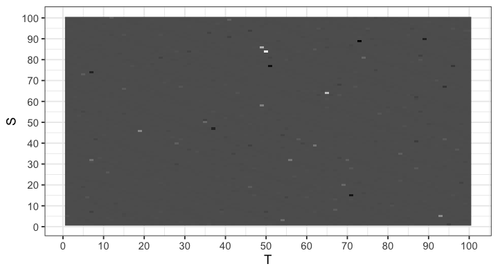
Figure 1: Grey scale image of noisy synthetic true data

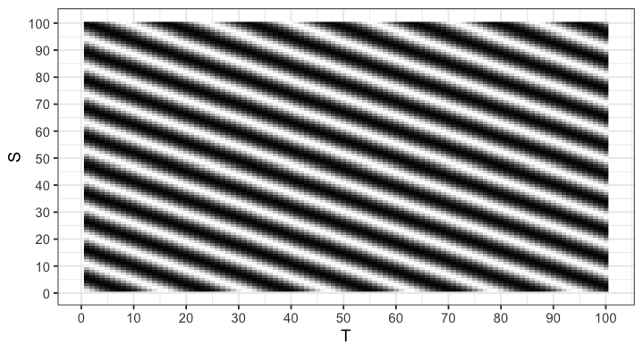
Figure 2: Grey scale image of Noiseless synthetic true data

Figure 3: Grey scale image of recovered data from LAD estimation

7 Conclusion

In this paper, we proposed a robust least absolute deviation estimators for estimating the parameters of a 2-dimensional sinusoidal model. We have established that the LAD estimators are strongly consistent and further have asymptotic normal distribution. It is observed that the LAD estimators of frequencies have a higher rate of convergence than the LAD estimators of amplitudes. It is observed in the simulations that in case of heavy tailed noise distribution and cases where outliers are present, the LAD method of estimation clearly outperforms least square method of estimation. While the performance of the non-robust LSEs break down under the presence of heavy tailed noise and fails to identify the correct parameters, the proposed LAD estimators provide robust estimates and performs satisfactorily under heavy tailed noise distributions. Synthetic data analysis of a texture data provides evidence of practical applicability of proposed LAD approach.

Appendix A Appendix

A.1 Proof of Thereom 1

For all $\theta\neq\theta_{0}$, define,

$$H_{T,S}(\theta)=Q_{T,S}(\theta)-Q_{T,S}(\theta_{0})$$

Now expanding $H_{T,S}(\theta)$ explicitly, we obtain,

$$\begin{split}H_{T,S}(\theta)&=\frac{1}{TS}\sum\limits_{t=1}^{T}\sum\limits_{s=1}^{S}\Bigg{\{}\Big{|}y(t,s)-A\cos(\lambda t+\mu s)-B\sin(\lambda t+\mu s)\Big{|}-{}\\ &\qquad\qquad\Big{|}y(t,s)-A^{0}\cos(\lambda^{0}t+\mu^{0}s)-B^{0}\sin(\lambda^{0}t+\mu^{0}s)\Big{|}\Bigg{\}}\end{split}$$

$$=\frac{1}{TS}\sum\limits_{t=1}^{T}\sum\limits_{s=1}^{S}\Bigg{\{}\Big{|}h_{t,s}(\theta)+\epsilon(t,s)\Big{|}-\Big{|}\epsilon(t,s)\Big{|}\Bigg{\}}=\frac{1}{TS}\sum\limits_{t=1}^{T}\sum\limits_{s=1}^{S}Z_{t,s}(\theta)$$

where, $Z_{t,s}=\Bigg{\{}\Big{|}h_{t,s}(\theta)+\epsilon(t,s)\Big{|}-\Big{|}\epsilon(t,s)\Big{|}\Bigg{\}}$ and $h_{t,s}(\theta)=A^{0}\cos(\lambda^{0}t+\mu^{0}s)+B^{0}\sin(\lambda^{0}t+\mu^{0}s)-A\cos(\lambda t+\mu s)-B\sin(\lambda t+\mu s)$. $Z_{t,s}$’s being only a function of i.i.d $\epsilon(t,s)$ are also independently distributed random variables. The proof of the theorem proceeds through essentially the two following important steps:

• $H_{T,S}(\theta)-\lim\limits_{T,S\rightarrow\infty}\mathbb{E}(H_{T,S}(\theta))\overset{a.s.}{\longrightarrow}0~{}~{}~{}\text{uniformly for all}~{}\theta\in\Theta$
  

• $\theta_{0}$ is the unique minimizer of $\lim\limits_{T,S\rightarrow\infty}\mathbb{E}(H_{T,S}(\theta))$.

We first show that $\mathbb{E}\Big{[}Z_{t,s}(\theta)\Big{]}<\infty$. Let us consider the case when $h_{t,s}(\theta)>0$.

$$\mathbb{E}\Big{[}Z_{t,s}(\theta)\Big{]} =\int Z_{t,s}(\theta)~{}dG(\epsilon(t,s))$$

$$=\int_{\epsilon(t,s)>0}h_{t,s}(\theta)dG(\epsilon(t,s))+\int_{-h_{t,s}(\theta)}^{0}\Big{(}h_{t,s}(\theta)+2\epsilon(t,s)\Big{)}dG(\epsilon(t,s)){}$$

$$\qquad\qquad\hskip 142.26378pt-\int\limits_{-\infty}^{-h_{t,s}(\theta)}h_{t,s}(\theta)dG(\epsilon(t,s))$$

$$=2\int_{-h_{t,s}(\theta)}^{0}\Big{(}h_{t,s}(\theta)+\epsilon(t,s)\Big{)}dG(\epsilon(t,s))~{}~{}(\text{since}~{}G(0)=\frac{1}{2})$$

$$=2\Big{[}h_{t,s}(\theta)G(0)-G\left(-h_{t,s}^{*}(\theta)\right)h_{t,s}(\theta)\Big{]}~{}~{}~{}\left(\text{with}-h_{t,s}^{*}(\theta)\in\left(0,-h_{t,s}(\theta)\right)\right).$$

The last equality in the above is obtained by applying integration by parts and integral mean value theorem. Similarly, for $h_{t,s}(\theta)<0$ proceeding same as above, we obtain,

$$\mathbb{E}\Big{[}Z_{t,s}(\theta)\Big{]}=2\Big{[}h_{t,s}(\theta)G(0)-G\left(-h_{t,s}^{**}(\theta)\right)h_{t,s}(\theta)\Big{]},~{}~{}\text{where},-h_{t,s}^{**}(\theta)\in\left(0,-h_{t,s}(\theta)\right).$$

Hence, it can be easily observed that $\mathbb{E}\Big{[}Z_{t,s}(\theta)\Big{]}<\infty$. Proceeding similarly as above we can show that Var$\Big{[}Z_{t,s}(\theta)\Big{]}<\infty$ and the bounds for both $\mathbb{E}\Big{[}Z_{t,s}(\theta)\Big{]}$ and Var$\Big{[}Z_{t,s}(\theta)\Big{]}$ are independent of $t$ and $s$.

Further, since $\Theta$ is compact $\exists~{}\Theta_{1},\ldots,\Theta_{k}$ such that $\Theta=\cup_{i=1}^{k}\Theta_{i}$ and $\sup\limits_{\theta\in\Theta_{i}}Z_{t,s}(\theta)-\inf\limits_{\theta\in\Theta_{i}}Z_{t,s}(\theta)<\frac{\epsilon}{2^{t}2^{s}}$ for each $\Theta_{i}$. Now,

$$\begin{split}H_{T,S}(\theta)-\lim_{T,S\rightarrow\infty}\mathbb{E}(H_{T,S}(\theta))&=\Bigg{[}\frac{1}{TS}\sum\limits_{t=1}^{T}\sum\limits_{s=1}^{S}Z_{t,s}(\theta)-\frac{1}{TS}\sum\limits_{t=1}^{T}\sum\limits_{s=1}^{S}\mathbb{E}\sup\limits_{\theta\in\Theta_{i}}Z_{t,s}(\theta)\Bigg{]}+{}\\ &\qquad\qquad\Bigg{[}\frac{1}{TS}\sum\limits_{t=1}^{T}\sum\limits_{s=1}^{S}\mathbb{E}\sup\limits_{\theta\in\Theta_{i}}Z_{t,s}(\theta)-\lim_{T,S\rightarrow\infty}\frac{1}{TS}\sum\limits_{t=1}^{T}\sum\limits_{s=1}^{S}\mathbb{E}Z_{t,s}(\theta)\Bigg{]}.\end{split}$$

We can show that the quantity $Z_{t,s}(\theta)$ is bounded by some quantity $M$ by using triangle inequality. Now using the compactness of the the parameter space and Kolmogorov’s strong law of large numbers(Billingsley, (1995)), we can show that

$$H_{T,S}(\theta)-\lim_{T,S\rightarrow\infty}\mathbb{E}(H_{T,S}(\theta))\overset{as.}{\longrightarrow}0~{}~{}~{}\text{uniformly for all}~{}\theta\in\Theta.$$

Now define $Q(\theta)=\lim_{T,S\rightarrow\infty}\mathbb{E}(H_{T,S}(\theta))$. It is easy to observe that $Q(\theta_{0})=0$. For all $\theta\neq\theta_{0}$, we obtain,

$$\begin{split}Q(\theta)&=\lim_{T,S\rightarrow\infty}\frac{2}{TS}\sum\limits_{Z_{t,s}(\theta)>0}\Big{[}h_{t,s}(\theta)\{G(0)-G\left(-h_{t,s}^{*}(\theta)\right)\}\Big{]}+{}\\ &\qquad\qquad\hskip 85.35826pt\frac{2}{TS}\sum\limits_{Z_{t,s}(\theta)<0}\Big{[}h_{t,s}(\theta)\{G(0)-G\left(-h_{t,s}^{**}(\theta)\right)\}\Big{]}\end{split}$$

$$\geq\lim_{T,S\rightarrow\infty}\frac{2}{TS}\sum\limits_{t=1}^{T}\sum\limits_{s=1}^{S}\big{|}h_{t,s}(\theta)\big{|}\min\bigg{\{}G\left(-h_{t,s}^{**}(\theta)\right)-\frac{1}{2},\frac{1}{2}-G\left(-h_{t,s}^{*}(\theta)\right)\bigg{\}}.$$

Now from Lemma 3.1 and (Oberhofer,, 1982, Lemma 4), it can be shown that $\lim\limits_{T,S\rightarrow\infty}\frac{1}{TS}\sum\limits_{t=1}^{T}\sum\limits_{s=1}^{S}\big{|}h_{t,s}(\theta)\big{|}^{2}=\frac{1}{2}A^{2}_{0}+\frac{1}{2}B^{2}_{0}+\frac{1}{2}A^{2}+\frac{1}{2}B^{2}>0$. Hence, we can conclude that $Q(\theta)$ has an unique minimizer in $\theta_{0}\in\Theta$. Thus, by using the sufficient conditions of Lemma 2.2 of White, (1980), we can conclude that $\hat{\theta}_{T,S}$ is strongly consistent for $\theta_{0}$, the true value of the parameter vector $\theta$.

A.2 Proof of Theorem 2

Let us consider,

$$Q_{T,S}(\theta) =\frac{1}{TS}\sum\limits_{t=1}^{T}\sum\limits_{s=1}^{S}\Big{|}y(t,s)-Acos(\lambda t+\mu s)-Bsin(\lambda t+\mu s)\Big{|}$$

$$=\frac{1}{TS}\sum\limits_{t=1}^{T}\sum\limits_{s=1}^{S}\big{|}h_{t,s}(\theta)+\epsilon(t,s)\big{|},$$

where, $h_{t,s}(\theta)=A^{0}cos(\lambda^{0}t+\mu^{0}s)+B^{0}sin(\lambda^{0}t+\mu^{0}s)-Acos(\lambda t+\mu s)-Bsin(\lambda t+\mu s)$. Note that $Q_{T,S}(\theta)$ is not a differentiable function. Since we shall make use of Taylor series expansion for finding the asymptotic normality of LAD estimators, we approximate the function $Q_{T,S}(\theta)$ by a function $Q^{*}_{T,S}(\theta)$, where,

$$Q^{*}_{T,S}(\theta)=\frac{1}{TS}\sum\limits_{t=1}^{T}\sum\limits_{s=1}^{S}\delta_{T,S}(h_{t,s}(\theta)+\epsilon(t,s)),$$

such that, $\lim_{x\rightarrow\infty}\delta_{T,S}(x)=|x|$ and $\delta_{T,S}(x)$ be a smooth function of $x$. We take

$$\delta_{T,S}(x) =\bigg{[}-\frac{1}{3}\beta^{2}_{T,S}x^{3}+\beta_{T,S}x^{2}+\frac{1}{3\beta_{T,S}}\bigg{]}\mathbb{I}_{\{0<x\leq\frac{1}{\beta_{T,S}}\}}+x\mathbb{I}_{\{x>\frac{1}{\beta_{T,S}}\}},$$

where, $\mathbb{I}_{B}$ denote the indicator function and the following conditions are satisfied:

• $\delta_{T,S}(x)$ is an even function of $x$, i.e. $\delta_{T,S}(x)=\delta_{T,S}(-x)$.

• $\beta_{T,S}$ is an appropriately chosen increasing function of both $T$ and $S$, simultaneously, such that $\lim\limits_{T,S\rightarrow\infty}\frac{1}{\beta_{T,S}}=0$ with $T^{2}S^{2}=o(\beta^{3}_{T,S})$ and $\beta_{T,S}=o(TS)$.

Note that, unlike $Q_{T,S}(\theta)$, $Q^{*}_{T,S}(\theta)$ is a twice continuously differentiable function. Let $\theta^{{}^{\prime}}_{T,S}=(A^{{}^{\prime}}_{T,S},B^{{}^{\prime}}_{T,S},\lambda^{{}^{\prime}}_{T,S},\mu^{{}^{\prime}}_{T,S})$ denote the minimizer of $Q^{*}_{T,S}(\theta)$. It can be shown easily, following the arguments of Appendix Section A.1, that $\theta^{{}^{\prime}}_{T,S}$ is strongly consistent for $\theta_{0}$. We first show that the minimum of $Q^{*}_{T,S}(\theta)$ is close to the minimum of $Q_{T,S}(\theta)$, for large $T,S$. To show this, let us consider the term $Q^{*}_{T,S}(\theta)-Q_{T,S}(\theta)$. Now,

$$Q^{*}_{T,S}(\theta)-Q_{T,S}(\theta) =\frac{1}{TS}\sum\limits_{t=1}^{T}\sum\limits_{s=1}^{S}\bigg{\{}\delta_{T,S}(h_{t,s}(\theta)+\epsilon(t,s))-|h_{t,s}(\theta)+\epsilon(t,s)|\bigg{\}}$$

$$=\begin{cases}\frac{1}{TS}\sum\limits_{t=1}^{T}\sum\limits_{s=1}^{S}\big{[}-\frac{1}{3}\beta^{2}_{T,S}u^{3}_{t,s}(\theta)+\beta_{T,S}u^{2}_{t,s}(\theta)+\frac{1}{3\beta_{T,S}}-u_{t,s}(\theta)\big{]},&{}\textstyle\\ \qquad\qquad\hskip 142.26378pt0<u_{t,s}(\theta)\leq\frac{1}{\beta_{T,S}}\\ \frac{1}{TS}\sum\limits_{t=1}^{T}\sum\limits_{s=1}^{S}\big{[}~{}~{}\frac{1}{3}\beta^{2}_{T,S}u^{3}_{t,s}(\theta)+\beta_{T,S}u^{2}_{t,s}(\theta)+\frac{1}{3\beta_{T,S}}+u_{t,s}(\theta)\big{]},&{}\textstyle\\ \qquad\qquad\hskip 142.26378pt-\frac{1}{\beta_{T,S}}<u_{t,s}(\theta)\leq 0\end{cases}$$

$$\begin{split}&=\frac{1}{TS}\sum\limits_{t=1}^{T}\sum\limits_{s=1}^{S}\bigg{[}-\frac{1}{3}\beta^{2}_{T,S}u^{3}_{t,s}(\theta)+\beta_{T,S}u^{2}_{t,s}(\theta)+\frac{1}{3\beta_{T,S}}-u_{t,s}(\theta)\bigg{]}{}\\ &\qquad\qquad\mathbb{I}_{\{0<u_{t,s}(\theta)\leq\frac{1}{\beta_{T,S}}\}}+\bigg{[}~{}~{}\frac{1}{3}\beta^{2}_{T,S}u^{3}_{t,s}(\theta)+\beta_{T,S}u^{2}_{t,s}(\theta)+{}\\ &\qquad\qquad\qquad\qquad\qquad\qquad\frac{1}{3\beta_{T,S}}+u_{t,s}(\theta)\bigg{]}\mathbb{I}_{\{-\frac{1}{\beta_{T,S}}<u_{t,s}(\theta)\leq 0\}}\end{split}$$

$$=\frac{1}{TS}\sum\limits_{t=1}^{T}\sum\limits_{s=1}^{S}W_{t,s}(\theta),\text{say,}$$

where, $u_{t,s}(\theta)=h_{t,s}(\theta)+\epsilon(t,s))$. Note that,

$$|W_{t,s}(\theta)| \leq\left(2\beta_{T,S}u^{2}_{t,s}(\theta)+\frac{2}{3\beta_{T,S}}\right)\mathbb{I}_{\{|u_{t,s}(\theta)|\leq\frac{1}{\beta_{T,S}}\}}$$

$$\leq\left(\frac{2}{\beta_{T,S}}+\frac{2}{3\beta_{T,S}}\right)\mathbb{I}_{\{|u_{t,s}(\theta)|\leq\frac{1}{\beta_{T,S}}\}}$$

$$=\frac{8}{3\beta_{T,S}}\mathbb{I}_{\{|u_{t,s}(\theta)|\leq\frac{1}{\beta_{T,S}}\}}.$$

Thus we have,

$$\mathbb{P}\left[|TS\left\{Q^{*}_{T,S}(\theta)-Q_{T,S}(\theta)\right\}|\geq\epsilon\right] \leq\frac{\mathbb{E}\left|TS\left\{Q^{*}_{T,S}(\theta)-Q_{T,S}(\theta)\right\}\right|}{\epsilon}~{}~{}~{}~{}$$

$$=\frac{\mathbb{E}\left|\sum\limits_{t=1}^{T}\sum\limits_{s=1}^{S}W_{t,s}(\theta)\right|}{\epsilon}$$

$$\leq\frac{\sum\limits_{t=1}^{T}\sum\limits_{s=1}^{S}\mathbb{E}\left|W_{t,s}(\theta)\right|}{\epsilon}~{}~{}~{}~{}$$

$$\leq\frac{8}{3\beta_{T,S}\epsilon}\sum\limits_{t=1}^{T}\sum\limits_{s=1}^{S}\mathbb{P}\left\{\left|u_{t,s}(\theta)\right|\leq\frac{1}{\beta_{T,S}}\right\}$$

$$=\frac{8}{3\beta_{T,S}\epsilon}\sum\limits_{t=1}^{T}\sum\limits_{s=1}^{S}\int\limits_{-h_{t,s}(\theta)-\frac{1}{\beta_{T,S}}}^{-h_{t,s}(\theta)+\frac{1}{\beta_{T,S}}}g(\epsilon(t,s))d\epsilon(t,s)$$

$$=\frac{16~{}\text{g}(c)~{}TS}{3\epsilon\beta^{2}_{T,S}}~{}~{}\text{(using integral mean value theorem)}$$

$$=\left(\frac{16~{}\text{g}(c)}{3\epsilon}\right)\left(\frac{\beta_{T,S}}{TS}\right)\left(\frac{T^{2}S^{2}}{\beta^{3}_{T,S}}\right)\rightarrow 0~{}~{}\text{as}~{}T,S\rightarrow\infty.$$

Thus, we can conclude that $TS\left\{Q^{*}_{T,S}(\theta)-Q_{T,S}(\theta)\right\}=o_{p}(1)$. Now since the parameter space $\Theta$ is compact and $Q^{*}_{T,S}(\theta)-Q_{T,S}(\theta)$ is continuous, we can say that there exists $\theta^{*}$ such that $TS\left\{Q^{*}_{T,S}(\theta^{*})-Q_{T,S}(\theta^{*})\right\}=\sup\limits_{\theta\in\Theta}TS\left\{Q^{*}_{T,S}(\theta)-Q_{T,S}(\theta)\right\}$. Hence we obtain from above,

$$\sup\limits_{\theta\in\Theta}TS\left\{Q^{*}_{T,S}(\theta)-Q_{T,S}(\theta)\right\}=o_{p}(1).$$ (5)

Now $\hat{\theta}_{T,S}$ being the minimizer of $Q_{T,S}(\theta)$, $Q_{T,S}(\hat{\theta}_{T,S})\leq Q_{T,S}(\theta^{{}^{\prime}}_{T,S})$. Hence from (5), we can conclude that,

$$TS\left\{Q^{*}_{T,S}(\hat{\theta}_{T,S})-Q^{*}_{T,S}(\theta^{{}^{\prime}}_{T,S})\right\}=o_{p}(1).$$ (6)

Now by Taylor series expansion upto $2^{\text{nd}}$ order, we have the following,

$$\begin{split}Q^{*}_{T,S}(\hat{\theta}_{T,S})=Q^{*}_{T,S}(\theta^{{}^{\prime}}_{T,S})+\nabla Q^{*}_{T,S}(\theta^{{}^{\prime}}_{T,S})(\hat{\theta}_{T,S}-\theta^{{}^{\prime}}_{T,S})+{}\\ \qquad\hskip 56.9055pt\frac{1}{2}(\hat{\theta}_{T,S}-\theta^{{}^{\prime}}_{T,S})^{T}\nabla^{2}Q^{*}_{T,S}(\bar{\theta}_{T,S})(\hat{\theta}_{T,S}-\theta^{{}^{\prime}}_{T,S});\end{split}$$ (7)

where, $\bar{\theta}_{T,S}=\eta\hat{\theta}_{T,S}+(1-\eta)\theta^{{}^{\prime}}_{T,S}$ and $\eta\in(0,1)$ and $\nabla Q^{*}_{T,S}(.)$ and $\nabla^{2}Q^{*}_{T,S}(.)$ denote the first and second order derivatives of $Q^{*}_{T,S}(.)$. Now since $\nabla Q^{*}_{T,S}(\theta^{{}^{\prime}}_{T,S})=0$, (7) gives

$$Q^{*}_{T,S}(\hat{\theta}_{T,S})=Q^{*}_{T,S}(\theta^{{}^{\prime}}_{T,S})+\frac{1}{2}(\hat{\theta}_{T,S}-\theta^{{}^{\prime}}_{T,S})^{T}\nabla^{2}Q^{*}_{T,S}(\bar{\theta}_{T,S})(\hat{\theta}_{T,S}-\theta^{{}^{\prime}}_{T,S}).$$ (8)

Realize that $\nabla^{2}Q^{*}_{T,S}(\bar{\theta}_{T,S})$ is a symmetric matrix and let $\lambda$ denote the smallest eigenvalue of the matrix $\nabla^{2}Q^{*}_{T,S}(\bar{\theta}_{T,S})$. Now using min-max theorem, we have,

$$(\hat{\theta}_{T,S}-\theta^{{}^{\prime}}_{T,S})^{T}\nabla^{2}Q^{*}_{T,S}(\bar{\theta}_{T,S})(\hat{\theta}_{T,S}-\theta^{{}^{\prime}}_{T,S})\geq\lambda(\hat{\theta}_{T,S}-\theta^{{}^{\prime}}_{T,S})^{T}(\hat{\theta}_{T,S}-\theta^{{}^{\prime}}_{T,S}).$$

Now from (8) we get

$$TS(\hat{\theta}_{T,S}-\theta^{{}^{\prime}}_{T,S})^{T}(\hat{\theta}_{T,S}-\theta^{{}^{\prime}}_{T,S})\leq\frac{2TS\left\{Q^{*}_{T,S}(\hat{\theta}_{T,S})-Q^{*}_{T,S}(\theta^{{}^{\prime}}_{T,S})\right\}}{\lambda}.$$

Now to prove that $\sqrt{TS}\|\hat{\theta}_{T,S}-\theta^{{}^{\prime}}_{T,S}\|=o_{p}(1)$, it is sufficient to show that $\lambda>0$ as we already have (6). Thus it is enough to show that the matrix $\nabla^{2}Q^{*}_{T,S}(\bar{\theta}_{T,S})$ is a positive definite, as $T,S\longrightarrow\infty$.

Let us now derive a result which will be useful to show the above stated positive definiteness. Note that

$$\begin{split}\mathbb{E}\left[\frac{1}{TS}\sum\limits_{t=1}^{T}\sum\limits_{s=1}^{S}\delta^{{}^{\prime\prime}}_{T,S}(\epsilon(t,s))\right]&=\frac{1}{TS}\sum\limits_{t=1}^{T}\sum\limits_{s=1}^{S}\bigg{[}\int_{0}^{\frac{1}{\beta_{T,S}}}(-2\beta^{2}_{T,S}x+2\beta_{T,S})\,dG(x)+{}\\ &\qquad\int_{-\frac{1}{\beta_{T,S}}}^{0}(2\beta^{2}_{T,S}x+2\beta_{T,S})\,dG(x)\bigg{]}\end{split}$$

$$=\frac{2}{TS}\sum\limits_{t=1}^{T}\sum\limits_{s=1}^{S}\left[g\left(\frac{1}{\beta_{T,S}}\right)-M\right]$$

$$=2g\left(\frac{1}{\beta_{T,S}}\right)-4M~{}~{}\longrightarrow~{}2g(0)~{}~{}\text{as}~{}~{}T,S\longrightarrow\infty;$$

where,

$$M=\int_{0}^{\frac{1}{\beta_{T,S}}}g^{{}^{\prime}}(x)\left(\beta^{2}_{T,S}\frac{x^{2}}{2}+\beta_{T,S}x\right)dx$$

and

$$|M|\leq C\int_{0}^{\frac{1}{\beta_{T,S}}}\left(\beta^{2}_{T,S}\frac{x^{2}}{2}+\beta_{T,S}x\right)dx=C\frac{2}{3\beta_{T,S}}\rightarrow 0~{}~{}\text{as}~{}~{}T,S\rightarrow\infty.$$

Therefore

$$\mathbb{E}\left[\frac{1}{TS}\sum\limits_{t=1}^{T}\sum\limits_{s=1}^{S}\delta^{{}^{\prime\prime}}_{T,S}(\epsilon(t,s))\right]=2g(0)+o(1).$$

Similarly, we can show that $\text{Vr}\left[\frac{1}{TS}\sum\limits_{t=1}^{T}\sum\limits_{s=1}^{S}\delta^{{}^{\prime\prime}}_{T,S}(\epsilon(t,s))\right]=o(1)$. Combining both of them and by using Markov’s inequality, we obtain that $\frac{1}{TS}\sum\limits_{t=1}^{T}\sum\limits_{s=1}^{S}\delta^{{}^{\prime\prime}}_{T,S}(\epsilon(t,s))=2g(0)+o_{p}(1)$.
Now let $\nabla^{2}Q^{*}_{T,S}(\bar{\theta}_{T,S})=((q_{i,j}))_{4\times 4}$. Using the lemma 3.2, straightforward calculations yields the following:

$$q_{1,1}=q_{2,2}=g(0)+o_{p}(1);~{}~{}~{}~{}~{}~{}q_{1,2}=o_{p}(1);$$

$$\frac{1}{T}q_{1,3}=\frac{1}{2}B^{0}g(0)+o_{p}(1);~{}~{}~{}~{}~{}\frac{1}{S}q_{1,4}=\frac{1}{2}B^{0}g(0)+o_{p}(1);$$

$$\frac{1}{T}q_{2,3}=-\frac{1}{2}A^{0}g(0)+o_{p}(1);~{}~{}~{}~{}~{}\frac{1}{S}q_{2,4}=-\frac{1}{2}A^{0}g(0)+o_{p}(1);$$

$$\frac{1}{T^{2}}q_{3,3}=\frac{1}{S^{2}}q_{4,4}=\frac{1}{3}({A^{0}}^{2}+{B^{0}}^{2})+o_{p}(1);~{}~{}~{}~{}~{}~{}\frac{1}{TS}q_{3,4}=\frac{1}{4}({A^{0}}^{2}+{B^{0}}^{2})+o_{p}(1).$$

Thus we have $\nabla^{2}Q^{*}_{T,S}(\bar{\theta}_{T,S})$ positive definite for $T,S\rightarrow\infty$. Further, we have

$$\sqrt{TS}\|\hat{\theta}_{T,S}-\theta^{{}^{\prime}}_{T,S}\|=o_{p}(1).$$

Under the same conditions, by using the Taylor series expansion of $Q^{*}_{T,S}(\theta)$ about only $\lambda$, we have

$$Q^{*}_{T,S}(\hat{\theta}_{T,S})-Q^{*}_{T,S}(\theta^{{}^{\prime}}_{T,S})=\frac{1}{2}(\hat{\lambda}_{T,S}-\lambda^{{}^{\prime}}_{T,S})^{2}\frac{\partial^{2}Q^{*}_{T,S}(\bar{\theta}_{T,S})}{\partial\lambda^{2}}.$$

We have that $T^{3}S(\hat{\lambda}_{T,S}-\lambda^{{}^{\prime}}_{T,S})^{2}=TS\left(Q^{*}_{T,S}(\hat{\theta}_{T,S})-Q^{*}_{T,S}(\theta^{{}^{\prime}}_{T,S})\right)+o_{p}(1)$. And from (6), we get

$$T^{\frac{3}{2}}S^{\frac{1}{2}}(\hat{\lambda}_{T,S}-\lambda^{{}^{\prime}}_{T,S})=o_{p}(1);$$

and

$$S^{\frac{3}{2}}T^{\frac{1}{2}}(\hat{\mu}_{T,S}-\mu^{{}^{\prime}}_{T,S})=o_{p}(1).$$

Since $Q_{TS}^{*}(\theta)$ is minimized at $\theta=\theta_{TS}^{{}^{\prime}}$; we apply multivariate mean value theorem on first derivative of $Q_{TS}^{*}(\theta)$ to get

$$\begin{split}(Q^{*}_{T,S})_{A^{0}}=-(Q^{*}_{T,S})_{\bar{A}\bar{A}}(A^{{}^{\prime}}_{T,S}-A^{0})+(Q^{*}_{T,S})_{\bar{A}\bar{B}}(B^{{}^{\prime}}_{T,S}-B^{0})+{}\\ (Q^{*}_{T,S})_{\bar{A}\bar{\lambda}}(\lambda^{{}^{\prime}}_{T,S}-\lambda^{0})+(Q^{*}_{T,S})_{\bar{A}\bar{\mu}}(\mu^{{}^{\prime}}_{T,S}-\mu^{0});\end{split}$$

$$\begin{split}(Q^{*}_{T,S})_{B^{0}}=-(Q^{*}_{T,S})_{\bar{B}\bar{A}}(A^{{}^{\prime}}_{T,S}-A^{0})+(Q^{*}_{T,S})_{\bar{B}\bar{B}}(B^{{}^{\prime}}_{T,S}-B^{0})+{}\\ (Q^{*}_{T,S})_{\bar{B}\bar{\lambda}}(\lambda^{{}^{\prime}}_{T,S}-\lambda^{0})+(Q^{*}_{T,S})_{\bar{B}\bar{\mu}}(\mu^{{}^{\prime}}_{T,S}-\mu^{0});\end{split}$$

$$\begin{split}(Q^{*}_{T,S})_{\lambda^{0}}=-(Q^{*}_{T,S})_{\bar{\lambda}\bar{A}}(A^{{}^{\prime}}_{T,S}-A^{0})+(Q^{*}_{T,S})_{\bar{\lambda}\bar{B}}(B^{{}^{\prime}}_{T,S}-B^{0})+{}\\ (Q^{*}_{T,S})_{\bar{\lambda}\bar{\lambda}}(\lambda^{{}^{\prime}}_{T,S}-\lambda^{0})+(Q^{*}_{T,S})_{\bar{\lambda}\bar{\mu}}(\mu^{{}^{\prime}}_{T,S}-\mu^{0});\end{split}$$

$$\begin{split}(Q^{*}_{T,S})_{\mu^{0}}=-(Q^{*}_{T,S})_{\bar{\mu}\bar{A}}(A^{{}^{\prime}}_{T,S}-A^{0})+(Q^{*}_{T,S})_{\bar{\mu}\bar{B}}(B^{{}^{\prime}}_{T,S}-B^{0})+{}\\ \hskip 56.9055pt(Q^{*}_{T,S})_{\bar{\mu}\bar{\lambda}}(\lambda^{{}^{\prime}}_{T,S}-\lambda^{0})+(Q^{*}_{T,S})_{\bar{\mu}\bar{\mu}}(\mu^{{}^{\prime}}_{T,S}-\mu^{0}).\end{split}$$

Where,

$$(Q^{*}_{T,S})_{A^{0}}=\frac{\partial Q^{*}_{T,S}(\theta)}{\partial A}\bigg{|}_{(A^{0},B^{0},\lambda^{0},\mu^{0})}~{}~{}\text{and }~{}~{}(Q^{*}_{T,S})_{\bar{A}\bar{B}}=\frac{\partial^{2}Q^{*}_{T,S}(\theta)}{\partial A\partial B}\bigg{|}_{(\bar{A}_{T,S},\bar{B}_{T,S},\bar{\lambda}_{T,S},\bar{\mu}_{T,S})}.$$

Note that here although the point $\bar{\theta}_{T,S}=(\bar{A}_{T,S},\bar{B}_{T,S},\bar{\lambda}_{T,S},\bar{\mu}_{T,S})$ is not same as that of $\bar{\theta}_{T,S}$ mentioned in (7) but in order to avoid extra notations, we adopt the same notation here to convey the same meaning as that of (7).
Thus, we have

$$\begin{split}\left(\sqrt{TS}(Q_{TS}^{*})_{A^{0}},\sqrt{TS}(Q_{TS}^{*})_{B^{0}},\frac{1}{\sqrt{TS}}(Q_{TS}^{*})_{\lambda^{0}},\frac{1}{\sqrt{TS}}(Q_{TS}^{*})_{\mu^{0}}\right)&={}\\ \left(\sqrt{TS}(A^{{}^{\prime}}_{T,S}-A^{0}),\sqrt{TS}(B^{{}^{\prime}}_{T,S}-B^{0}),T^{\frac{3}{2}}S^{\frac{1}{2}}(\lambda^{{}^{\prime}}_{T,S}-\lambda^{0}),S^{\frac{3}{2}}T^{\frac{1}{2}}(\mu^{{}^{\prime}}_{T,S}-\mu^{0})\right)Z_{T,S};\end{split}$$

where,

$$Z_{T,S}=\begin{pmatrix}(Q^{*}_{T,S})_{\bar{A}\bar{A}}&(Q^{*}_{T,S})_{\bar{B}\bar{A}}&T^{-1}S^{-1}(Q^{*}_{T,S})_{\bar{\lambda}\bar{A}}&T^{-1}S^{-1}(Q^{*}_{T,S})_{\bar{\mu}\bar{A}}\\ (Q^{*}_{T,S})_{\bar{A}\bar{B}}&(Q^{*}_{T,S})_{\bar{B}\bar{B}}&T^{-1}S^{-1}(Q^{*}_{T,S})_{\bar{\lambda}\bar{B}}&T^{-1}S^{-1}(Q^{*}_{T,S})_{\bar{\mu}\bar{B}}\\ T^{-1}(Q^{*}_{T,S})_{\bar{A}\bar{\lambda}}&T^{-1}(Q^{*}_{T,S})_{\bar{B}\bar{\lambda}}&T^{-2}S^{-1}(Q^{*}_{T,S})_{\bar{\lambda}\bar{\lambda}}&T^{-2}S^{-1}(Q^{*}_{T,S})_{\bar{\mu}\bar{\lambda}}\\ S^{-1}(Q^{*}_{T,S})_{\bar{A}\bar{\mu}}&S^{-1}(Q^{*}_{T,S})_{\bar{B}\bar{\mu}}&S^{-2}T^{-1}(Q^{*}_{T,S})_{\bar{\lambda}\bar{\mu}}&S^{-2}T^{-1}(Q^{*}_{T,S})_{\bar{\mu}\bar{\mu}}\end{pmatrix}.$$

Now we know that $\delta^{{}^{\prime}}_{T,S}(x)=\left[-\beta^{2}_{T,S}x^{2}+2\beta_{T,S}x\right]\mathbb{I}_{\left\{0<x\leq\frac{1}{\beta_{T,S}}\right\}}+\mathbb{I}_{\left\{x\geq\frac{1}{\beta_{T,S}}\right\}}~{}\text{and}~{}\delta^{{}^{\prime}}_{T,S}(-x)=-\delta^{{}^{\prime}}_{T,S}(x)$. Hence by applying Markov’s inequality it can be easily shown that,

$$\sqrt{TS}(Q_{TS}^{*})_{A^{0}}=\frac{1}{\sqrt{TS}}\sum\limits_{t=1}^{T}\sum\limits_{s=1}^{S}(-\cos(\lambda t+\mu s))\left(\mathbb{I}_{\{\epsilon(t,s)\geq\frac{1}{\beta_{T,S}}\}}-\mathbb{I}_{\{\epsilon(t,s)\leq-\frac{1}{\beta_{T,S}}\}}\right)+o_{p}(1)$$ (9)

$$\sqrt{TS}(Q_{TS}^{*})_{B^{0}}=\frac{1}{\sqrt{TS}}\sum\limits_{t=1}^{T}\sum\limits_{s=1}^{S}(-\sin(\lambda t+\mu s))\left(\mathbb{I}_{\{\epsilon(t,s)\geq\frac{1}{\beta_{T,S}}\}}-\mathbb{I}_{\{\epsilon(t,s)\leq-\frac{1}{\beta_{T,S}}\}}\right)+o_{p}(1)$$ (10)

$$\begin{split}\frac{1}{\sqrt{TS}}(Q_{TS}^{*})_{\lambda^{0}}=\frac{1}{\sqrt{T^{3}S}}\sum\limits_{t=1}^{T}\sum\limits_{s=1}^{S}(A^{0}t\sin(\lambda t+\mu s)-B^{0}t\cos(\lambda t+\mu s)){}\\ \left(\mathbb{I}_{\{\epsilon(t,s)\geq\frac{1}{\beta_{T,S}}\}}-\mathbb{I}_{\{\epsilon(t,s)\leq-\frac{1}{\beta_{T,S}}\}}\right)+o_{p}(1)\end{split}$$ (11)

$$\begin{split}\frac{1}{\sqrt{TS}}(Q_{TS}^{*})_{\mu^{0}}=\frac{1}{\sqrt{S^{3}T}}\sum\limits_{t=1}^{T}\sum\limits_{s=1}^{S}(A^{0}s\sin(\lambda t+\mu s)-B^{0}s\cos(\lambda t+\mu s)){}\\ \left(\mathbb{I}_{\{\epsilon(t,s)\geq\frac{1}{\beta_{T,S}}\}}-\mathbb{I}_{\{\epsilon(t,s)\leq-\frac{1}{\beta_{T,S}}\}}\right)+o_{p}(1)\end{split}$$ (12)

The sums (9)-(12) are of the form $\sum\limits_{t=1}^{T}\sum\limits_{s=1}^{S}U_{t,s}$, $U_{t,s}$ appropriately defined as in the corresponding equation. For (9) we have,

$$\mathbb{E}(U_{t,s}) = \sum\limits_{t=1}^{T}\sum\limits_{s=1}^{S}(-\cos(\lambda t+\mu s))\mathbb{E}\left(\mathbb{I}_{\{\epsilon(t,s)\geq\frac{1}{\beta_{T,S}}\}}-\mathbb{I}_{\{\epsilon(t,s)\leq-\frac{1}{\beta_{T,S}}\}}\right)$$

$$= \sum\limits_{t=1}^{T}\sum\limits_{s=1}^{S}(-\cos(\lambda t+\mu s))\left(\int\limits_{\frac{1}{\beta_{T,S}}}^{\infty}d(G(\epsilon(t,s)))-\int\limits^{-\frac{1}{\beta_{T,S}}}_{-\infty}d(G(\epsilon(t,s)))\right)$$

$$= \sum\limits_{t=1}^{T}\sum\limits_{s=1}^{S}(-\cos(\lambda t+\mu s))\left(1-G\left(\frac{1}{\beta_{T,S}}\right)-G\left(-\frac{1}{\beta_{T,S}}\right)\right).$$

As $T,S\longrightarrow\infty$, we have $\frac{1}{\beta_{T,S}}\longrightarrow 0$; therefore, $\mathbb{E}(U_{t,s})=o(1)$. Similarly for the equations (10)-(12), we can show that,

$$\mathbb{E}(U_{t,s})=o(1).$$ (13)

Now proceeding similarly as above we can show that,

$$\text{Var}\left(\sum\limits_{t=1}^{T}\sum\limits_{s=1}^{S}U_{t,s}\right) =\begin{cases}\frac{1}{2}+o(1),&\text{for \eqref{eq:14},\eqref{eq:15}}\\ \\ \frac{{A^{0}}^{2}+{B^{0}}^{2}}{6}+o(1),&\text{for \eqref{eq:16},\eqref{eq:17}}\end{cases}$$

$$=B_{T,S},~{}~{}\text{(say)}.$$

Further, we can show that for the above random variable $U_{t,s}$, the Lindeberg condition, i.e. $\lim\limits_{T,S\rightarrow\infty}\frac{1}{B_{T,S}}\sum\limits_{t=1}^{T}\sum\limits_{s=1}^{S}\mathbb{E}\left(U_{t,s}^{2}\mathbb{I}_{\left\{|U_{T,S}|\geq\epsilon\sqrt{B_{T,S}}\right\}}\right)=0$ holds and therefore by applying Lindeberg-Feller Central theorem (Van der Vaart, (1998)) we can conclude that,

$\sqrt{TS}(Q_{TS}^{*})_{A^{0}}$, $\sqrt{TS}(Q_{TS}^{*})_{B^{0}},\frac{1}{\sqrt{TS}}(Q_{TS}^{*})_{\lambda^{0}}$ and $\frac{1}{\sqrt{TS}}(Q_{TS}^{*})_{\mu^{0}}$ converges in distribution to $N(0,1/2)$, $N(0,1/2)$, $N\left(0,\frac{{A^{0}}^{2}+{B^{0}}^{2}}{6}\right)$ and $N\left(0,\frac{{A^{0}}^{2}+{B^{0}}^{2}}{6}\right)$, respectively.

Now we make use of the Cramer-Wald device to find the asymptotic joint distribution of $\left(\sqrt{TS}(Q_{TS}^{*})_{A^{0}},\sqrt{TS}(Q_{TS}^{*})_{B^{0}},\frac{1}{\sqrt{TS}}(Q_{TS}^{*})_{\lambda^{0}},\frac{1}{\sqrt{TS}}(Q_{TS}^{*})_{\mu^{0}}\right)$. Consider the linear combination,

$$A_{T,S}=a_{1}(Q_{TS}^{{}^{\prime}})_{A^{0}}+a_{2}(Q_{TS}^{{}^{\prime}})_{B^{0}}+a_{3}(Q_{TS}^{{}^{\prime}})_{\lambda^{0}}+a_{4}(Q_{TS}^{{}^{\prime}})_{\mu^{0}};$$ (14)

where, $a_{1},a_{2},a_{3}~{}\text{and}~{}a_{4}$ are arbitrary real numbers. Now using (13), we have for 14,

$$\mathbb{E}(A_{T,S})=o(1)$$

and by using Lemma 3.1 we can easily derive that

$$\begin{split}\text{Var}(A_{T,S})=\frac{a^{2}_{1}}{2}+\frac{a^{2}_{2}}{2}+\frac{{A^{0}}^{2}+{B^{0}}^{2}}{6}a^{2}_{3}+\frac{{A^{0}}^{2}+{B^{0}}^{2}}{6}a^{2}_{4}+{}\\ \qquad\frac{B^{0}}{2}a_{1}a_{3}+\frac{B^{0}}{2}a_{1}a_{4}+\frac{A^{0}}{2}a_{2}a_{3}+\frac{A^{0}}{2}a_{2}a_{4}+\frac{{A^{0}}^{2}+{B^{0}}^{2}}{4}a_{3}a_{4}+o(1).\end{split}$$

We can express the random variable $A_{T,S}$ as $\sum\limits_{t=1}^{T}\sum\limits_{s=1}^{S}U_{t,s}$ and using the Lindeberg condition it is possible to apply the central limit theorem to $A_{T,S}$. Further, by applying the Cramer-Wald device we obtain that,
$\left(\sqrt{TS}(Q_{TS}^{*})_{A^{0}},\sqrt{TS}(Q_{TS}^{*})_{B^{0}},\frac{1}{\sqrt{TS}}(Q_{TS}^{*})_{\lambda^{0}},\frac{1}{\sqrt{TS}}(Q_{TS}^{*})_{\mu^{0}}\right)Z^{-1}_{T,S}$ converges in distribution to $N_{4}(0,\Sigma)$; where

$$\Sigma=\begin{pmatrix}\frac{1}{2}&0&\frac{B^{0}}{4}&\frac{B^{0}}{4}\\ \\ 0&\frac{1}{2}&-\frac{A^{0}}{4}&-\frac{A^{0}}{4}\\ \\ \frac{B^{0}}{4}&-\frac{A^{0}}{4}&\frac{{A^{0}}^{2}+{B^{0}}^{2}}{6}&\frac{{A^{0}}^{2}+{B^{0}}^{2}}{8}\\ \\ \frac{B^{0}}{4}&-\frac{A^{0}}{4}&\frac{{A^{0}}^{2}+{B^{0}}^{2}}{8}&\frac{{A^{0}}^{2}+{B^{0}}^{2}}{6}\end{pmatrix}.$$

It is easy to show that $\lim\limits_{T,S\rightarrow\infty}Z_{T,S}=2g(0)\Sigma$.
Now,

$$\begin{split}\left(\sqrt{TS}(\hat{A}_{T,S}-A^{0}),\sqrt{TS}(\hat{B}_{T,S}-B^{0}),T^{\frac{3}{2}}S^{\frac{1}{2}}(\hat{\lambda}_{T,S}-\lambda^{0}),S^{\frac{3}{2}}T^{\frac{1}{2}}(\hat{\mu}^{{}^{\prime}}_{T,S}-\mu^{0})\right)&={}\text{ \>\> }\\ \qquad\qquad\underbrace{\left(\sqrt{TS}(A^{{}^{\prime}}_{T,S}-A^{0}),\sqrt{TS}(B^{{}^{\prime}}_{T,S}-B^{0}),T^{\frac{3}{2}}S^{\frac{1}{2}}(\lambda^{{}^{\prime}}_{T,S}-\lambda^{0}),S^{\frac{3}{2}}T^{\frac{1}{2}}(\mu^{{}^{\prime}}_{T,S}-\mu^{0})\right)}_{A}+{}\\ \qquad\qquad\underbrace{\left(\sqrt{TS}(\hat{A}-A^{{}^{\prime}}_{T,S}),\sqrt{TS}(\hat{B}-B^{{}^{\prime}}_{T,S}),T^{\frac{3}{2}}S^{\frac{1}{2}}(\hat{\lambda}-\lambda^{{}^{\prime}}_{T,S}),S^{\frac{3}{2}}T^{\frac{1}{2}}(\hat{\mu}-\mu^{{}^{\prime}}_{T,S})\right)}_{B}\end{split}$$

Now (B) goes to $0$ in probability and (A) has the same asymptotic distribution as that of $\left(\sqrt{TS}(Q_{TS}^{*})_{A^{0}},\sqrt{TS}(Q_{TS}^{*})_{B^{0}},\frac{1}{\sqrt{TS}}(Q_{TS}^{*})_{\lambda^{0}},\frac{1}{\sqrt{TS}}(Q_{TS}^{*})_{\mu^{0}}\right)Z_{T,S}^{-1}$, i.e. has asymptotic distribution as $N_{4}\left(0,\frac{1}{4g^{2}(0)}\Sigma^{-1}\right)$. Applying the Slutsky’s lemma, we obtain the desired result.

A.3 Proof of Theorem 3

Let $\hat{\theta}^{4p\times 1}_{T,S}=(\hat{A}_{T,S;1},\hat{B}_{T,S;1},\hat{\lambda}_{T,S;1},\hat{\mu}_{T,S;1},\dots,\hat{A}_{T,S;p},\hat{B}_{T,S;p},\hat{\lambda}_{T,S;p},\hat{\mu}_{T,S;p})^{{}^{\prime}}$ be the LAD estimator obtained by minimizing the quantity given by (2). Proceeding similarly as in the proof of Theorem 3.2, we can show that,

$$H_{T,S}(\theta)-\lim\limits_{T,S\rightarrow\infty}\mathbb{E}(H_{T,S}(\theta))\overset{\text{a.s.}}{\longrightarrow}0~{}~{}~{}\text{uniformly}~{}~{}\forall~{}~{}\theta\in\Theta,$$

and also that the true value $\theta_{0}$ is the unique global minimizer of $\lim\limits_{T,S\rightarrow\infty}\mathbb{E}(H_{T,S}(\theta))$. Hence, from Lemma 2.2 of White, (1980), strong consistency of $\hat{\theta}_{T,S}$ follows.

References

• Andrews and Hunt, (1977) Andrews, H. C. and Hunt, B. R. (1977). Digital image restoration. Prentice-Hall Signal Processing Series, Englewood Cliffs: Prentice-Hall.
• Bansal et al., (1999) Bansal, N. K., Hamedani, G. G., and Zhang, H. (1999). Non-linear regression with multidimensional indices. Statistics & Probability Letters, 45(2):175–186.
• Billingsley, (1995) Billingsley, P. (1995). Probability and measure, 3rd edition. Wiley series in probability and mathematical statistics, pages 289–290.
• Clark and Scharf, (1994) Clark, M. P. and Scharf, L. L. (1994). Two-dimensional modal analysis based on maximum likelihood. IEEE Transactions on Signal Processing, 42(6):1443–1452.
• Cohen and Francos, (2002) Cohen, G. and Francos, J. A. (2002). Least squares estimation of 2-d sinusoids in colored noise: Asymptotic analysis. IEEE Transactions on Information Theory, 48(8):2243–2252.
• Dudgeon, (1977) Dudgeon, D. E. (1977). Fundamentals of digital array processing. Proceedings of the IEEE, 65(6):898–904.
• Francos et al., (1993) Francos, J. M., Meiri, A. Z., and Porat, B. (1993). A unified texture model based on a 2-d wold-like decomposition. IEEE Transactions on Signal Processing, 41(8):2665–2678.
• Grover et al., (2022) Grover, R., Sharma, A., Delcourt, T., and Kundu, D. (2022). Computationally efficient algorithm for frequency estimation of a two-dimensional sinusoidal model. Circuits, Systems, and Signal Processing, 41(1):346–371.
• Hua, (1992) Hua, Y. (1992). Estimating two-dimensional frequencies by matrix enhancement and matrix pencil. IEEE Transactions on Signal Processing, 40(9):2267–2280.
• Kim et al., (2000) Kim, T. S., Kim, H. K., and Choi, S. H. (2000). Asymptotic properties of lad estimators of a nonlinear time series regression model. Journal of the Korean Statistical Society, 29:2:187–199.
• Kundu and Gupta, (1998) Kundu, D. and Gupta, R. D. (1998). Asymptotic properties of the least squares estimators of a two dimensional model. Metrika, 48(2):83–97.
• Kundu and Mitra, (1996) Kundu, D. and Mitra, A. (1996). Asymptotic properties of the least squares estimates of 2-d exponential signals. Multidimensional Systems and Signal Processing, 7:135–150.
• Kundu and Nandi, (2003) Kundu, D. and Nandi, S. (2003). Determination of discrete spectrum in a random field. Statistica Neerlandica, 57(2):258–284.
• Mitra and Stoica, (2002) Mitra, A. and Stoica, P. (2002). Asymptotic cramer-rao bound for 2-d superimposed exponential signals. Multidimensional Systems and Signal Processing, 13:317–331.
• Oberhofer, (1982) Oberhofer, W. (1982). The consistency of nonlinear regression minimizing the $l_{1}$ norm. Annals of Statistics, 10:316–319.
• Odendaal et al., (1994) Odendaal, J. W., Barnard, E., and Pistorius, C. W. I. (1994). Two-dimensional superresolution radar imaging using the music algorithm. IEEE Transactions on Antennas and Propagation, 42(10):1386–1391.
• Prasad et al., (2008) Prasad, A., Kundu, D., and Mitra, A. (2008). Sequential estimation of two dimensional sinusoidal models. Journal of Statistical Planning and Inference, 138:1297–1313.
• Rao et al., (1994) Rao, C. R., Zhao, L. C., and Zhou, B. (1994). Maximum likelihood estimation of 2-d superimposed exponential signals. IEEE Transactions on Signal Processing, 42:1795–1802.
• Rossi and Willsky, (1984) Rossi, D. J. and Willsky, A. S. (1984). Reconstruction from projections based on detection and estimation of objects, pts. i and 11: performance analysis and robustness analysis. IEEE Transactions on Acoustics Speech and Signal Processing, 32:886–906.
• Van der Vaart, (1998) Van der Vaart, A. W. (1998). Asymptotic statistics. Cambridge University Press, pages 20–21.
• Van der Veen et al., (1998) Van der Veen, A., Vanderveen, M. C., and Paulraj, A. (1998). Joint angle and delay estimation using shift-invariance techniques. IEEE Transactions on Signal Processing, 46(2):405–418.
• Vinogradov, (1954) Vinogradov, I. M. (1954). The method of trigonometrical sums in the theory of numbers(translated from russian).
• White, (1980) White, H. (1980). Nonlinear regression on cross-section data. Econometrica, 48:721–746.
• Zhang and Mandrekar, (2001) Zhang, H. and Mandrekar, V. (2001). Estimation of hidden frequencies for 2d stationary processes. Journal of Time Series Analysis, 22(5):613–629.