Relegation-free closed-form perturbation theory and the domain of secular motions in the Restricted 3-Body Problem

Abstract

We propose a closed-form (i.e. without expansion in the orbital eccentricities) scheme for computations in perturbation theory in the restricted three-body problem (R3BP) when the massless particle is in an orbit exterior to the one of the primary perturber. Starting with a multipole expansion of the barycentric (Jacobi-reduced) Hamiltonian, we carry out a sequence of normalizations in Delaunay variables by Lie series, leading to a secular Hamiltonian model without use of relegation. To this end, we introduce a book-keeping analogous to the one proposed in [1] for test particle orbits interior to the one of the primary perturber, but here adapted, instead, to the case of exterior orbits. We give numerical examples of the performance of the method in both the planar circular and the spatial elliptic restricted three-body problem, for parameters pertinent to the Sun-Jupiter system. In particular, we demonstrate the method’s accuracy in terms of reproducibility of the orbital elements’ variations far from mean-motion resonances. As a basic outcome of the method, we show how, using as criterion the size of the series’ remainder, we reach to obtain an accurate semi-analytical estimate of the boundary (in the space of orbital elements) where the secular Hamiltonian model arrived at after eliminating the particle’s fast degree of freedom provides a valid approximation of the true dynamics.

Keywords: Celestial mechanics – Astrodynamics – R3BP – Closed-form – No relegation – Secular motion

1 Introduction

As opposed to the usual (Laplace-Lagrange) theory, closed-form perturbation theory [11] provides a framework for series calculations in perturbed Keplerian problems without expansions in powers of the bodies’ orbital eccentricities. This is mainly motivated by the necessity to construct secular models for sufficiently eccentric orbits, like those of many asteroids, in our solar system, or the planets in extrasolar planetary systems.

The efficiency of the usual series methods of expansion in the orbital eccentricities is limited by the fact that the inversion of Kepler’s equation in powers of the eccentricity converges only up to the so-called Laplace limit $e_{L}\approx 0.66274$ [6]. Generally, such convergence slows down way before this value (around $e\sim 0.3-0.4$ in many applications). In order to address this issue, closed form perturbation theory aims at solving in ‘closed-form’ the homological equation by which the Lie generating function is computed at every perturbative step (see for example [3, 5]). The process is far from being priceless: a major obstruction appears when the kernel of the homological equations contains addenda beyond the Keplerian terms. The most common such addendum ([11]) is the centrifugal term $-\nu H$, where $\nu$ is the angular frequency in a frame co-rotating with the primary perturber, and $H$ is the Delaunay action equal to the particle’s angular momentum in the direction of the axis of rotation. In the case of a planet’s orbiter, $\nu$ is equal to the planet’s rotation frequency, and the problem appears for all non-axisymmetric terms (tesseral harmonics) of the planet’s multipole potential. In the R3BP, instead, $\nu$ represents the mean motion of the primary perturber (e.g. Jupiter in the Sun-Jupiter system), while the problem appears in a similar way after introducing a multipole expansion of the disturbing function in the particle’s Hamiltonian.

An algorithm to overcome the above issue, called the relegation algorithm, has been proposed in works by Deprit, Palaciań and collaborators [15, 4, 7, 2, 13]. Briefly, given a quasi-integrable Hamiltonian $H=H_{0}+\varepsilon H_{1}$, where $\varepsilon$ is a small parameter, suppose that $H_{0}=H_{0}^{\prime}+H_{0}^{\prime\prime}$, where, in a domain in phase space we have that $H_{0}^{\prime}$ yields the dominant contribution to the Hamiltonian flow of $H_{0}$ versus the $H_{0}^{\prime\prime}$ term. In usual perturbation theory, we seek to partly normalize the perturbation $H_{1}$ via a sequence of canonical transformations defined by generating functions $\chi^{(r)}$, $r=1,2,\ldots$ satisfying a homological equation of the form $\{H_{0},\chi^{(r)}\}+h_{1}^{(r)}=0$, where $\{\cdot,\cdot\}$ denotes the Poisson bracket between two functions of the canonical variables and $h_{1}^{(r)}$ is a term in the Hamiltonian to be normalized. In the relegation technique, we use instead the equation $\{H_{0}^{\prime},\chi^{(r)}\}+h_{1}^{(r)}=0$, i.e., letting only the dominant function $H_{0}^{\prime}$ in the kernel of the homological equation. Such a choice stems mostly from motives of algorithmic convenience. For example, identifying $H_{0}^{\prime}$ with the Keplerian term (when $\nu$ is small) leads to a homological equation that can be solved in closed form (we set, instead, $H_{0}^{\prime}=-\nu H$ when $\nu$ is large). However, all Poisson brackets of $\chi^{(r)}$ with the part $H_{0}^{\prime\prime}$ left out of the kernel lead to terms which need to be ‘relegated’, i.e., pushed to normalization in subsequent steps. For reasons explained in detail in [14], only a finite number or relegation steps can be performed before reaching a point beyond which the scheme generates divergent sequences of terms (see also [13]). This implies that the process necessarily stops after some steps, leading to a finite, albeit possibly quite small remainder.

Relegation is a technique particularly suitable to the limiting situation of a strongly hierarchical problem, when the integrable part $H_{0}$ depends on a frequency vector involving $n$ frequencies $\omega=(\omega_{1},\ldots,\omega_{n})$ out of which one, say $\omega_{i}$ for some $i$ with $1\leq i\leq n$ is significantly larger in absolute value than the rest. In particular, the harmonics $\cos(k\cdot\varphi)$ in the Hamiltonian whose normalization can be ‘relegated’ should satisfy $|k_{i}\omega_{i}|\gg|k_{j}\omega_{j}|$, $j=1,\ldots,n$, $j\neq i$, for every integer $k_{i},k_{j}\in\mathbb{Z}\setminus\{0\}$ (assuming also the non-resonant condition $k\cdot\omega\neq 0$, $k=(k_{1},\ldots,k_{n})$). For example, as explained in [14] in the simple case with $n=2$ and $\omega_{2}\gg\omega_{1}$, the generating function $\chi^{(N)}$ produced after $N$ relegation steps contains terms with coefficients growing as a geometric sequence with ratio $k_{1}\omega_{1}/k_{2}\omega_{2}$. Thus, relagation is limited to those terms for which the above ratio is smaller than unity. This includes most harmonics of low Fourier order in the Hamiltonian perturbation when $\omega_{2}\gg\omega_{1}$, but only few when the two frequencies become comparable in size. Hence, by construction, relegation has limited applicability in this latter, non-hierarchical, case.

Variants of the relegation technique have been discussed in literature to address perturbed Keplerian problems in which the gravitational potential is due to an extended body expanded in spherical harmonics (e.g. [7, 10]). To address the non-hierarchical case, a techique similar to the one of the present paper is discussed in [7], referring to the averaging of the tesseral harmonics in the case of the Earth’s artificial satellites. In the case of the R3BP, instead, Cavallari and Efthymiopoulos [1] discuss a relegation-free algorithm for the elimination of short-period terms in the particle’s Hamiltonian, when the orbit of the particle (e.g. an asteroid) is totally interior to the orbit of the primary perturber (e.g. Jupiter). We are aware of no relegation-free algorithm proposed in literature which addresses, instead, the case when the particle’s orbit is exterior to the orbit of the primary perturber. Providing such an algorithm, discussing some of its important differences with past-proposed algorithms, as well as checking its limits of applicability, constitutes the primary goal of our present paper.

The R3BP is defined by the motion of a body $\mathcal{P}$ of negligible mass in the gravitational field of two massive bodies $\mathcal{P}_{0}$ (the primary or central body) and $\mathcal{P}_{1}$ (the secondary or primary perturber), which perform a motion $r_{1}(t)$ either elliptic in the more general version (ER3BP) or circular (CR3BP). The starting point for our analysis in the sequel is the Hamiltonian of the model, obtained after reduction via Jacobi coordinates $(R,P)$.. Expressing time through the secondary’s mean anomaly $M_{1}=n_{1}t$, where $n_{1}$ is the mean motion of the secondary, and canonically conjugating $M_{1}$ with a dummy action variable $J_{1}$ allows to express the Hamiltonian as

$$\mathcal{H}(R,M_{1},P,J_{1})=\frac{\left\lVert P\right\rVert^{2}}{2}-\frac{\mathcal{G}m_{0}}{\left\lVert R+\mu r_{1}(M_{1})\right\rVert}-\frac{\mathcal{G}m_{1}}{\left\lVert R-(1-\mu)r_{1}(M_{1})\right\rVert}+n_{1}J_{1}\;,$$ (1)

where $\mathcal{G}$ is the gravitational constant and

$$\mu=\dfrac{m_{1}}{m_{0}+m_{1}}\in(0,1/2]\;$$

is the mass parameter;

$$r_{1}(M_{1})=a_{1}\left(\cos E_{1}(M_{1})-e_{1},\sqrt{1-e_{1}^{2}}\sin E_{1}(M_{1}),0\right)$$ (2)

is the elliptic revolution of $\mathcal{P}_{0}-\mathcal{P}_{1}$ around their barycenter with eccentricity $e_{1}$ and semi-major axis $a_{1}$, in which the dependence of the system’s eccentric anomaly $E_{1}\in\mathbb{T}=\mathbb{R}/(2\pi\mathbb{Z})$ on the mean anomaly $M_{1}\in\mathbb{T}$ is given through Kepler’s equation according to standard two-body problem setting; $(R=(X,Y,Z),P=(P_{X},P_{Y},P_{Z}))\in T^{*}(\mathbb{R}^{3}\setminus\{-\mu r_{1},(1-\mu)r_{1}\})$ is the position-momentum couple of $\mathcal{P}$ and the phase space is endowed with standard symplectic form $dP_{X}\wedge dX+dP_{Y}\wedge dY+dP_{Z}\wedge dZ+dJ_{1}\wedge dM_{1}$.
We make use then of Delaunay elements $(\ell,g,h,L,G,H)$, defined by

$$L =\sqrt{\mathcal{G}m_{0}a}\;, \ell =M\;,$$

$$G =L\sqrt{1-e^{2}}\;, g =\omega\;,$$ (3)

$$H =G\cos i\;, h =\Omega\;,$$

where $a,e,i,M,\Omega,\omega$ stand for the semi-major axis, the eccentricity, the inclination, the mean anomaly, the longitude of the ascending node, the argument of pericenter of the particle.

A key ingredient of the method proposed below is the following: similarly as in [1], we introduce a book-keeping symbol $\sigma$ with numerical value equal to $1$, whose role is to organize the perturbative scheme so as to successively normalize terms of similar order of smallness, treating together all small quantities of the problem, i.e.,

• the eccentricities $e$, $e_{1}$ (when $e_{1}\neq 0$),

• the mass ratio $\mu$,

• the semi-major axis fluctuation $\delta L$ around the mean $L_{*}$ for a particular particle trajectory.

The book-keeping symbol acts by assigning powers $\sigma^{1}$ and $\sigma^{\nu_{1}}$, $\sigma^{\nu}$, $\sigma^{\nu}$ respectively, for non-zero natural numbers $\nu$, $\nu_{1}$ defined below, to all the terms in the original Hamiltonian as well as in the Hamiltonian produced after every normalization step. Given this baseline, we arrive (in Section 2) to the following result: we demonstrate that, for $k_{\mu},k_{\text{mp}}\in\mathbb{N}\setminus\{0\}$ with $k_{\mu}>1$, the combination of expansions of (1) up to $\mu^{k_{\mu}}$ and $(\left\lVert r_{1}\right\rVert/\left\lVert R\right\rVert)^{k_{\text{mp}}}$ is canonically conjugate by $\nu(k_{\mu}-1)$ near-identity transformations to a secular model, obtained as a normal form with respect to the fast angles $\ell,M_{1}$

$$\mathscr{H}(\ell,g,h,M_{1},\delta L,G,H,J_{1})=\mathscr{H}_{0}(g,h,\delta L,G,H,J_{1})+\mathscr{R}(\ell,g,h,M_{1},\delta L,G,H)\;,$$ (4)

with

$$\mathscr{H}_{0}=n_{*}\delta L+n_{1}J_{1}+\sum_{l=\nu}^{\nu k_{\mu}-1}\sum_{p\in\mathbb{Z}^{2}}c_{l,p}(\delta L,e,i;\mu,L_{*},a_{1},e_{1})\cos(p_{1}g+p_{2}h)\sigma^{l}\;,$$ (5)

$$\mathscr{R}=\sum_{s\in\mathbb{Z}^{4}}d_{\nu k_{\mu},s}(E_{1},\delta L,e,i;\mu,L_{*},a_{1},e_{1})\cos(s_{1}f+s_{2}g+s_{3}h+s_{4}E_{1})\sigma^{\nu k_{\mu}}\\ +\mathcal{O}\left(\sigma^{\nu k_{\mu}+1};\left(\frac{\left\lVert r_{1}\right\rVert}{\left\lVert R\right\rVert}\right)^{k_{\text{mp}}+1}\right)\;.$$ (6)

The dependencies $f=f(\ell,\delta L,G)$ for the true anomaly, $e=e(\delta L,G)$ and $i=i(G,H)$ are implied in all the above expressions; $c_{l,p},d_{\nu k_{\mu},s}$ are real coefficients. A crucial point is the way by which the positive integers $\nu=\nu(e_{*},\mu)\geq 1$, $\nu_{1}=\nu_{1}(e_{*},e_{1})\geq 1$ are chosen. As detailed below, these integers, which regulate the book-keeping scheme, are suitably tuned on the basis of a selected reference value $e_{*}\in(0,1)$:

$$\nu=\left\lceil\frac{\log_{10}\mu}{\log_{10}e_{*}}\right\rceil\;,\quad\quad\nu_{1}=\left\lceil\frac{\log_{10}e_{1}}{\log_{10}e_{*}}\right\rceil\;,$$ (7)

where $\lceil\cdot\rceil$ is the ceiling function. The normalizing scheme leading to (4) is local: knowing that the semi-major axis is preserved under the flow of the (secular) normal form, we introduce the splitting $L=L_{*}+\delta L$, where $L_{*}=\sqrt{\mathcal{G}m_{0}a_{*}}\gg\delta L$, $n_{*}=\sqrt{\mathcal{G}m_{0}}a_{*}^{-3/2}$ is a targeted reference value for the semi-major axis $a_{*}$, and expand the Hamiltonian in powers of $\delta L$, rendering $\delta L$ the new action variable canonically conjugated to the particle’s mean anomaly.

Given the above, the normalization algorithm provides a sequence of Lie generating functions $\chi^{(j)}_{\nu+j-1}=\mathcal{O}(\sigma^{\nu+j-1})$, $j=1,\ldots,\nu(k_{\mu}-1)$, which yields the Lie canonical transformation allowing to recursively normalize all terms depending on the angles $f$ and $E_{1}$ in the Hamiltonian. The normalizing trasformations are possible to define for values of the frequencies $n_{*}$ (mean motion of the particle at the semi-major axis $a_{*}$) and $n_{1}$ far from mean-motion resonances (see Remark 3). Furthermore, the generating functions are computed as solutions of a homological equation of the form

$$\{\mathscr{Z}_{0},\chi_{\nu+j-1}^{(j)}\}+\mathscr{R}_{\nu+j-1,\nu+j-1}^{(j-1)}=\mathcal{O}(\sigma^{\nu+j-1})\;,$$ (8)

where $\mathscr{Z}_{0}=n_{*}\delta L+n_{1}J_{1}$ and $\mathscr{R}_{\nu+j-1,\nu+j-1}^{(j-1)}\sim\sigma^{\nu+j-1}$ collects the trigonometric monomials of $\mathcal{O}(\sigma^{\nu+j-1})$ depending on at least one of the two anomalies. The key to obtaining a closed-form solution for (8) is, precisely, the appropriate choice of a $\mathcal{O}(\sigma^{\nu+j-1})$ remainder left in the second hand of the equation. In words, we do not seek for an exact cancellation of the terms $\mathscr{R}_{\nu+j-1,\nu+j-1}^{(j-1)}$, but only for an approximate cancellation, leading to a remainder, which, however, is of higher order in book-keeping, and, hence, possible to reduce at subsequent steps.

As discussed in Section 3, a relevant outcome of the analysis of the behavior of the remainder obtained by the above method stems from an estimation of the optimal number of normalization steps $j_{opt}$, where the remainder becomes of order $\nu+j_{opt}-1$ in the book-keeping parameter, with $j_{opt}\leq\nu(k_{\mu}-1)$. The value of $j_{opt}$ is defined as the one where the error bound $\mathscr{E}^{(j)}(a_{*},e_{*})=\sum_{\nu+j\leq l\leq\nu k_{\mu},s}|d_{l,s}^{(j)}|\geq\|\mathscr{R}^{(j)}_{\nu+j}\|_{\infty}=\sup|\mathscr{R}^{(j)}_{\nu+j}|$ becomes minimum, with $\mathscr{R}^{(j)}_{\nu+j}=\mathcal{O}(\sigma^{\nu+j})$ and $d_{l,s}^{(j)}$ as in $\eqref{eqn:R}$ after $j$ normalization steps. As typical in perturbation theory, the value of $j_{opt}$ depends on the chosen reference values $(a_{*},e_{*})$. With the present method one can then obtain a map of the size of the optimal remainder as a function of $(a_{*},e_{*})$ in the semi-plane $a>a_{1}$. Using this information, we compute the limiting locus uniting all points in $(a_{*},e_{*})$ such that the normal form computation yields no improvement with increasing number of normalization steps, i.e., where $j_{opt}=1$. Comparing with numerical stability maps obtained with the Fast Lyapunov Indicator (FLI) [9], one sees that, the limiting locus found semi-analytically essentially coincides with the numerical (FLI map) limit where no harmonic in the Hamiltonian associated with one of the exterior mean-motion resonances affects the dynamics. As a consequence, all motions in the sub-domain of the plane $(a_{*},e_{*})$ below the limiting locus are stable in the secular sense, i.e., protected against instabilities caused by short-period resonant effects. For this reason, we identify this locus as the border of the domain of secular motions, and substantiate the fact that its semi-analytical computation (through the normal forms) yields results in precise agreement with those found by the heuristic definition of the same border via the fully numerical (FLI) computation of stability maps.

The paper is structured as follows. Section 2 presents step-by-step the algorithm that gives rise to (5) and (6), supplemented with the formulas for the Poisson algebra in Keplerian elements used in all closed-form computations. Section 3 is devoted to a numerical investigation of the method’s accuracy for an asteroid in the Sun-Jupiter system, first in the spatial ER3BP, and then in the planar CR3BP; in the latter case, the computations are short enough to allow for a specification of the optimal normalization order in a grid of values in the $(a_{*},e_{*})$ plane, leading to the semi-analytical determination of the border of the domain of secular motions. Section 4 summarizes the basic conclusions of the present study and gives some relevant comments for future work.

2 The closed-form method for the outermost R3BP

2.1 Multipole expansion of the perturbation

Referring to section 1, let $\mathcal{H}$ be given in barycentric Cartesian coordinates as in (1):

$$\mathcal{H}=\frac{\left\lVert P\right\rVert^{2}}{2}+n_{1}J_{1}-\mathcal{G}m_{0}\mathcal{R}\;,$$ (9)

Assuming $\left\lVert r_{1}\right\rVert/\left\lVert R\right\rVert<1$, we carry out a multipole expansion of the function $\mathcal{R}(R,M_{1})$ in powers of the ratio $\left\lVert r_{1}\right\rVert/\left\lVert R\right\rVert<1$:

$$\begin{split}\mathcal{R}&=\frac{1}{\left\lVert R+\mu r_{1}\right\rVert}+\frac{\mu}{1-\mu}\frac{1}{\left\lVert R+(1-\mu)r_{1}\right\rVert}\\ &=\frac{1}{\left\lVert R\right\rVert}\large\Bigg{(}\sum_{l=0}^{\infty}\binom{-1/2}{l}\left(\frac{2\mu r_{1}\cdot R}{\left\lVert R\right\rVert^{2}}+\mu^{2}\left(\frac{\left\lVert r_{1}\right\rVert}{\left\lVert R\right\rVert}\right)^{2}\right)^{l}\\ &\quad+\frac{\mu}{1-\mu}\sum_{l=0}^{\infty}\binom{-1/2}{l}\left(-\frac{2(1-\mu)r_{1}\cdot R}{\left\lVert R\right\rVert^{2}}+(1-\mu)^{2}\left(\frac{\left\lVert r_{1}\right\rVert}{\left\lVert R\right\rVert}\right)^{2}\right)^{l}\large\Bigg{)}\\ &=\frac{1}{1-\mu}\frac{1}{\left\lVert R\right\rVert}+\mathcal{O}\left(\left(\frac{\left\lVert r_{1}\right\rVert}{\left\lVert R\right\rVert}\right)^{2}\right)\;.\end{split}$$ (10)

where, for $\beta\in\mathbb{R}$

$$\binom{\beta}{l}=\frac{\beta(\beta-1)\cdots(\beta-l+1)}{l!}$$

indicates the generalized binomial coefficient (equal to $1$ for $l=0$).

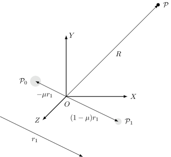
Figure 1: Representation of the R3BP in the barycentric frame (or equivalently in Jacobi variables) with $\left\lVert R\right\rVert>\left\lVert r_{1}\right\rVert$.

Remark 1.

For $l=1$ in Eq.(10) the coefficients of the dipole term $(r_{1}\cdot R)/\left\lVert R\right\rVert^{3}$ in the two sums in the r.h.s. of the equation cancel each other exactly. Thus, no dipole term appears in the disturbing function. This is a consequence of the choice of Jacobi coordinates.

2.2 Canonical form of the Hamiltonian

Performing an extra series expansion in powers of $\mu<1$ yields the standard nearly-integrable form

$$\mathcal{H}=\mathcal{H}_{0}+\mu\mathcal{H}_{1}\;,$$ (11)

where the Keplerian part reads

$$\mathcal{H}_{0}=\frac{\left\lVert P\right\rVert^{2}}{2}-\frac{\mathcal{G}m_{0}}{\left\lVert R\right\rVert}+n_{1}J_{1}\;$$ (12)

and the disturbing function becomes

$$\mathcal{H}_{1}=-\frac{\mathcal{G}m_{0}}{\left\lVert R\right\rVert}\large\Bigg{(}\sum_{l=0}^{\infty}\mu^{l}+\sum_{l=1}^{\infty}\mu^{l-1}\binom{-1/2}{l}\left(\frac{2r_{1}\cdot R}{\left\lVert R\right\rVert^{2}}+\mu\left(\frac{\left\lVert r_{1}\right\rVert}{\left\lVert R\right\rVert}\right)^{2}\right)^{l}\\ +\sum_{l=1}^{\infty}(1-\mu)^{l-1}\binom{-1/2}{l}\left(-\frac{2r_{1}\cdot R}{\left\lVert R\right\rVert^{2}}+(1-\mu)\left(\frac{\left\lVert r_{1}\right\rVert}{\left\lVert R\right\rVert}\right)^{2}\right)^{l}\large\Bigg{)}\;.$$ (13)

We now move to Delaunay action-angle variables (1) by replacing into (11) the relationships

$$\mathcal{H}_{0}=-\frac{\mathcal{G}m_{0}}{2a}+n_{1}J_{1}\;,$$ (14)

$$\left\lVert R\right\rVert=\frac{a(1-e^{2})}{1+e\cos f}\;,$$ (15)

$$r_{1}\cdot R=a_{1}\left\lVert R\right\rVert\Big{(}(\cos E_{1}-e_{1})\left(\cos h\cos(g+f)-\sin h\sin(g+f)\cos i\right)\\ +\sqrt{1-e_{1}^{2}}\sin E_{1}\left(\sin h\cos(g+f)+\cos h\sin(g+f)\cos i\right)\Big{)}\;$$ (16)

as well as (2) for the vector $r_{1}$. We get

$$\mathcal{H}=-\frac{\mathcal{G}m_{0}}{2a}+n_{1}J_{1}+\mu\mathcal{H}_{1}(f,g,h,E_{1},a,e,i;\mu,a_{1},e_{1})\;.$$ (17)

Remark 2.

Only the square of the norm $\left\lVert r_{1}\right\rVert^{2}=r_{1}\cdot r_{1}$ is required in Eq.(13), while the norm $\left\lVert R\right\rVert$ appears only in the denominator of the above equation, in powers equal to or higher than quadratic. Then equations (15) and (2), respectively dependent on $f$ and $E_{1}$, lead to a representation of the disturbing function as a sum of trigonometric polynomials depending on harmonics of the form $\cos(s_{1}f+s_{2}g+s_{3}h+s_{4}E_{1})$. This is a key ingredient of the closed-form method, i.e., working with the angles $f$ and $E_{1}$, instead of the mean anomalies $M,M_{1}$, no series reversion of Kepler’s equation is used throughout the whole perturbative scheme.

In order to avoid relegation, our method discussed below works locally, by constructing a model for the secular Hamiltonian valid for a particle’s semi-major axis varying as $a=a_{*}+\delta a(t)$, i.e., by a small quantity $\delta L$ around some reference value $a_{*}$. By standard secular theory, we have the estimate $\delta a=\mathcal{O}(\mu)$ far from mean-motion resonances. Formally, introducing the new canonical variable $\delta L$ as

$$L=L_{*}+\delta L=\sqrt{\mathcal{G}m_{0}a_{*}}+\frac{1}{2}\sqrt{\frac{\mathcal{G}m_{0}}{a_{*}}}\delta a+\mathcal{O}(\delta a^{2})\;.$$ (18)

and expanding the Hamiltonian in powers of the quantity $\delta L$ around $L_{*}$, we obtain

$$\begin{split}\mathcal{H}&=-\frac{\mathcal{G}^{2}m_{0}^{2}}{2L_{*}^{2}}\sum_{l=0}^{\infty}\binom{-2}{l}\left(\frac{\delta L}{L_{*}}\right)^{l}+n_{1}J_{1}+\mu\sum_{l=0}^{\infty}\frac{1}{l!}\left.\frac{\partial^{l}\mathcal{H}_{1}}{\partial L^{l}}\right|_{L=L_{*}}\delta L^{l}\\ &=n_{*}\delta L+n_{1}J_{1}+\mu\left(\left.\mathcal{H}_{1}\right|_{\delta L=0,\text{ }\mu=0}+\left.\frac{\partial\mathcal{H}_{1}}{\partial\delta L}\right|_{\delta L=0,\text{ }\mu=0}\delta L\right)+\mathcal{O}(\mu^{2},\delta L^{2})\;,\end{split}$$ (19)

where a constant term $-\mathcal{G}^{2}m_{0}^{2}/(2L_{*}^{2})$ was dropped from the expansion. The constant $n_{*}=\mathcal{G}^{2}m_{0}^{2}/L_{*}^{3}$ is equal to the particle’s mean motion under Keplerian orbit at the semi-major axis $a_{*}$.

Remark 3.

The choice of the reference value $a_{*}$ determines the kind of divisors appearing in the normalization procedure. In the present paper, we deal only with the ‘non-resonant’ case, in which the frequencies $n_{*}$ and $n_{1}$ satisfy no-commensurability condition. For example, to be far from any resonance we may require that $n_{*}$ and $n_{1}$ satisfy a diophantine condition

$$|k_{*}n_{*}+k_{1}n_{1}|>\frac{\gamma}{|k|^{\tau}}\;,\quad\forall k=(k_{*},k_{1})\in\mathbb{Z}^{2}\setminus\{0\}$$ (20)

with $|k|=|k_{*}|+|k_{1}|$ and some suitable $\gamma>0$, $\tau>1$.
However, the algorithm presented below can be readily extended to cases of mean-motion resonance. We leave the details for a future work, noting only that in resonant cases we have the estimate $\delta L=\mathcal{O}(\mu^{1/2})$, instead of $\mathcal{O}(\mu)$. The effect of approaching close to a mean-motion resonance with the present series is seen, instead, as a rise in the value of the series’ remainder, caused by (non-zero) small divisors in the series (as visible, for example, in Fig. 7 discussed in section 3 below).

2.3 Poisson structure and book-keeping

2.3.1 Poisson bracket formulas

All steps of closed-form perturbation theory involve Poisson brackets between differentiable functions of the form $F(\ell,g,h,M_{1},\delta L,G,H,J_{1})\in\mathcal{C}^{\infty}(\mathbb{T}^{4}\times D)$, $D\subset\mathbb{R}^{4}$ being an open set, whose dependence on the variables $\ell$, $M_{1}$, $G$ and $H$ is given in implicit form through the functions $f(\ell,\delta L,G)$, $E_{1}(M_{1},e(\delta L,G))$, $e(\delta L,G)$, $\iota_{c}(G,H)=\cos i(G,H)$, $\iota_{s}(G,H)=\sin i(G,H)$, $\eta(\delta L,G)=\sqrt{1-e(\delta L,G)^{2}}$, $\left\lVert r_{1}\right\rVert(M_{1})=a_{1}(1-e_{1}\cos E_{1}(M_{1}))$, and $\phi_{1}(M_{1})=E_{1}(M_{1},e(\delta L,G))-M_{1}$. The Poisson bracket between two functions $F_{1},F_{2}$ of the above form is computed by the formulas

$$\begin{split}\left\{F_{1},F_{2}\right\}&={\text{d}F_{1}\over\text{d}\ell}{\text{d}F_{2}\over\text{d}\delta L}+{\text{d}F_{1}\over\text{d}g}{\text{d}F_{2}\over\text{d}G}+{\text{d}F_{1}\over\text{d}h}{\text{d}F_{2}\over\text{d}H}+{\text{d}F_{1}\over\text{d}M_{1}}{\text{d}F_{2}\over\text{d}J_{1}}\\ &-{\text{d}F_{1}\over\text{d}\delta L}{\text{d}F_{2}\over\text{d}\ell}-{\text{d}F_{1}\over\text{d}G}{\text{d}F_{2}\over\text{d}g}-{\text{d}F_{1}\over\text{d}h}{\text{d}F_{2}\over\text{d}H}-{\text{d}F_{1}\over\text{d}J_{1}}{\text{d}F_{2}\over\text{d}M_{1}}\end{split}$$ (21)

implemented to the closed-form version of the functions $F_{1},F_{2}$. The closed-form version of a function $F$ is defined as:

$$F=F(f,g,h,E_{1},\delta L,e,\eta,\iota_{c},\iota_{s},J_{1})\;.$$ (22)

The derivatives in the canonical variables of a function $F$ as in Eq.(21) are computed by the chain rule formulas

$$\frac{\text{d}F}{\text{d}\ell}=\frac{\partial F}{\partial f}\frac{\partial f}{\partial\ell}\;,$$ (23)

$$\frac{\text{d}F}{\text{d}g}=\frac{\partial F}{\partial g}\;,$$ (24)

$$\frac{\text{d}F}{\text{d}h}=\frac{\partial F}{\partial h}\;,$$ (25)

$$\frac{\text{d}F}{\text{d}M_{1}}=\left(\frac{\partial F}{\partial E_{1}}+\frac{\partial F}{\partial\left\lVert r_{1}\right\rVert}\frac{\text{d}\left\lVert r_{1}\right\rVert}{\text{d}E_{1}}+\frac{\partial F}{\partial\phi_{1}}\right)\frac{\text{d}E_{1}}{\text{d}M_{1}}-\frac{\partial F}{\partial\phi_{1}}\;,$$ (26)

$$\frac{\text{d}F}{\text{d}\delta L}=\frac{\partial F}{\partial f}\frac{\partial f}{\partial\delta L}+\frac{\partial F}{\partial\delta L}+\frac{\partial F}{\partial e}\frac{\partial e}{\partial\delta L}+\frac{\partial F}{\partial\eta}\frac{\partial\eta}{\partial\delta L}\;,$$ (27)

$$\frac{\text{d}F}{\text{d}G}=\frac{\partial F}{\partial f}\frac{\partial f}{\partial G}+\frac{\partial F}{\partial e}\frac{\partial e}{\partial G}+\frac{\partial F}{\partial\eta}\frac{\partial\eta}{\partial G}+\frac{\partial F}{\partial\iota_{c}}\frac{\partial\iota_{c}}{\partial G}+\frac{\partial F}{\partial\iota_{s}}\frac{\partial\iota_{s}}{\partial G}\;,$$ (28)

$$\frac{\text{d}F}{\text{d}H}=\frac{\partial F}{\partial\iota_{c}}\frac{\partial\iota_{c}}{\partial H}+\frac{\partial F}{\partial\iota_{s}}\frac{\partial\iota_{s}}{\partial H}\;,$$ (29)

$$\frac{\text{d}F}{\text{d}J_{1}}=\frac{\partial F}{\partial J_{1}}\;,$$ (30)

where

$$\frac{\partial f}{\partial\ell}=\frac{(1+e\cos f)^{2}}{\eta^{3}}\;,$$ (31)

$$\frac{\text{d}\left\lVert r_{1}\right\rVert}{\text{d}E_{1}}=a_{1}e_{1}\sin E_{1}\;,$$ (32)

$$\frac{\text{d}E_{1}}{\text{d}M_{1}}=\frac{a_{1}}{\left\lVert r_{1}\right\rVert}\;,$$ (33)

$$\frac{\partial f}{\partial\delta L}=\frac{1}{L}\left(\frac{2\sin f}{e}+\frac{\sin(2f)}{2}\right)=\frac{1}{L_{*}}\left(\frac{2\sin f}{e}+\frac{\sin(2f)}{2}\right)\left(1-\frac{\delta L}{L_{*}}\right)+\mathcal{O}(\delta L^{2})\;,$$ (34)

$$\frac{\partial e}{\partial\delta L}=\frac{\eta^{2}}{eL}=\frac{\eta^{2}}{eL_{*}}\left(1-\frac{\delta L}{L_{*}}\right)+\mathcal{O}(\delta L^{2})\;,$$ (35)

$$\frac{\partial\eta}{\partial\delta L}=-\frac{\eta}{L}=-\frac{\eta}{L_{*}}\left(1-\frac{\delta L}{L_{*}}\right)+\mathcal{O}(\delta L^{2})\;,$$ (36)

$$\begin{aligned} \frac{\partial f}{\partial G}&=-\frac{1}{\eta L}\left(\frac{2\sin f}{e}+\frac{\sin(2f)}{2}\right)\\ &=-\frac{1}{\eta L_{*}}\left(\frac{2\sin f}{e}+\frac{\sin(2f)}{2}\right)\left(1-\frac{\delta L}{L_{*}}\right)+\mathcal{O}(\delta L^{2})\;,\end{aligned}$$

$$\frac{\partial e}{\partial G}=-\frac{\eta}{eL}=-\frac{\eta}{eL_{*}}\left(1-\frac{\delta L}{L_{*}}\right)+\mathcal{O}(\delta L^{2})\;,$$ (37)

$$\frac{\partial\eta}{\partial G}=\frac{1}{L}=\frac{1}{L_{*}}\left(1-\frac{\delta L}{L_{*}}\right)+\mathcal{O}(\delta L^{2})\;,$$ (38)

$$\frac{\partial\iota_{c}}{\partial G}=-\frac{\iota_{c}}{\eta L}=-\frac{\iota_{c}}{\eta L_{*}}\left(1-\frac{\delta L}{L_{*}}\right)+\mathcal{O}(\delta L^{2})\;,$$ (39)

$$\frac{\partial\iota_{s}}{\partial G}=-\frac{1-\iota_{s}^{2}}{\eta L\iota_{s}}=-\frac{1-\iota_{s}^{2}}{\eta L_{*}\iota_{s}}\left(1-\frac{\delta L}{L_{*}}\right)+\mathcal{O}(\delta L^{2})\;,$$ (40)

$$\frac{\partial\iota_{c}}{\partial H}=\frac{1}{\eta L}=\frac{1}{\eta L_{*}}\left(1-\frac{\delta L}{L_{*}}\right)+\mathcal{O}(\delta L^{2})\;,$$ (41)

$$\frac{\partial\iota_{s}}{\partial H}=-\frac{\iota_{c}}{\eta L\iota_{s}}=-\frac{\iota_{c}}{\eta L_{*}\iota_{s}}\left(1-\frac{\delta L}{L_{*}}\right)+\mathcal{O}(\delta L^{2})\;.$$ (42)

A sketch of the derivation of the above formulas can be found in Appendix A. They are strictly valid with $e\in(0,1)$, $i\in(0,\pi)$. However, several cancellations lead to no singular behavior of the Poisson bracket formulas arising throughout the various perturbative steps also when $e=0$ or $i=0$.

2.3.2 Book-keeping: Hamiltonian

We introduce in the series a book-keeping symbol $\sigma$ (see [5] for an introduction to the book-keeping technique), with numerical value $\sigma=1$, whose role is to provide a grouping of all the various terms in the series according to their ‘order of smallness’. Hence, a group of terms with common factor $\sigma^{l}$, $l\in\mathbb{Z}$, indicates a term considered as of the ‘$l$-th order of smallness’.

Since in our series there are several small quantities, we introduce a book-keeping scheme allowing to simultaneously deal with all small quantities while maintaining the closed-form character of the series. To this end, we make the following substitutions, called ‘book-keeping rules’, within the initial Hamiltonian:

• BK-Rule 1: $e\leadsto\sigma^{1}e=\sigma e$ (not applicable to the quantity $e^{2}$ within $\eta=\sqrt{1-e^{2}}$),

• BK-Rule 2: $\eta\leadsto\sigma^{0}\eta=\eta$,

• BK-Rule 3: $\mu\leadsto\sigma^{\nu}\mu$, with $\nu$ as in Eq.(7),

• BK-Rule 4: $e_{1}\leadsto\sigma^{\nu_{1}}e_{1}$, with $\nu_{1}$ as in Eq.(7) (not applicable to the quantity $e_{1}^{2}$ within $\eta_{1}\coloneqq\sqrt{1-e_{1}^{2}}$),

• BK-Rule 5: $\frac{1}{\eta^{2}}\leadsto\left(\frac{1}{\eta^{2}}-1\right)\sigma^{2}+1$,

• BK-Rule 6: $\eta_{1}\leadsto(\eta_{1}-1)\sigma^{2\nu_{1}}+1$,

• BK-Rule 7: $\delta L^{\lambda}\leadsto\sigma^{l\nu}\delta L^{\lambda}$ with $l=\begin{cases}\lambda\;,&\text{if }\delta L^{\lambda}\text{ comes from }\mathcal{H}_{1}\;,\\ \lambda-1\;,&\text{if }\delta L^{\lambda}\text{ comes from }\mathcal{H}_{0}\;,\end{cases}\hskip 5.69054pt\lambda\in\mathbb{N}\setminus\{0\}$.

Since $\sigma=1$, the above substitutions affect the structure of the series only at the formal level, and can be substituted directly into the original Hamiltomian, whereby they propagate at subsequent normalization steps once these steps are organized in successive powers $\sigma,\sigma^{2}$, etc., of the book-keeping symbol. The BK-Rules 1 to 7 above are justified on physical ground as well as on motives of algorithmic convenience. In particular:

- BK-Rule 1 implies that, despite the use of closed-form formulas, the basic small quantity in powers of which the series are organized is the eccentricity of the test particle.

- BK-Rule 3 implies that a factor $\mu$ in front of a series term should be treated as of comparable order of smallness as a term of order $e^{\nu}$, with $\nu$ given by Eq.(7). Similarly, BK-Rule 4 implies that a term containing a factor $e_{1}$ raised to some power should be treated as of comparable order of smallness with a term $e^{\nu}_{1}$ raised to the same power. Note that the eccentricity $e$ is a quantity variable in time, so that to compute the exponents $\nu,\nu_{1}$ we need to use, for any examined trajectory, a reference value $e_{*}$ yielding an estimate of the overall level of eccentricity all along the orbital evolution for that trajectory. Note that, by standard secular theory we have $e(t)=e_{*}+\mathcal{O}(\mu)$ if $e_{*}$ is close to the mean eccentricity (see also discussion at the introduction). Note finally that we obtain exponents $\nu,\nu_{1}\geq 1$ in the typical case in which $e>\mu$ and $e\geq e_{1}$. These inequalities arise naturally in the case of small bodies in highly eccentric orbits perturbed by some planet of, say, our solar system, which are the cases of main interest in applying the present method (see, nevertheless, Remark 4 on the treatment of cases where the above conditions are not met).

- BK-Rule 7 stems from the estimate $\delta L=\mathcal{O}(\delta a)=\mathcal{O}(\mu)$ holding for the oscillations in semi-major axis of trajectories far from mean-motion resonances (as already pointed outin the latter case, instead, we have in general $\delta L=\mathcal{O}(\delta a)=\mathcal{O}(\mu^{1/2})$ and the corresponding rule has to be adapted accordingly). The lowering of the book-keeping power by one for within $H_{0}$ is introduced for reasons of algorithmic convenience, i.e., in order to maintain $n_{*}\delta L$ in the kernel of the homological equation.

- BK-Rules 5 and 6 imply just a partition of the unity aiming at keeping the perturbative scheme in closed-form while splitting the corresponding expressions (involving $\eta$ and $\eta_{1}$ respectively) in two parts, of orders $\mathcal{O}(1)$ and $\mathcal{O}(e^{2})$, or $\mathcal{O}(e_{1}^{2})$.

2.3.3 Book-keeping: Poisson structure

Some of the formulas in Subsection 2.3.1 imply differentiation with respect to $e$ through the corresponding partial derivatives in (27), (28), thus yielding a lowering of the power of the eccentricity in some terms arising through Poisson brackets at consecutive steps of perturbation theory. To account for this fact, similarly as in [1] we introduce the use of the book-keeping symbol $\sigma$ in the formulas of the Poisson algebra as follows: first, we re-write the derivatives with respect to the angles $\ell,g,h,M_{1}$ as

$$\frac{\text{d}F}{\text{d}\ell}=\frac{\partial F}{\partial f}\frac{\partial f}{\partial\ell}\frac{a_{1}(1-e_{1}\sigma^{\nu_{1}}\cos E_{1})}{\left\lVert r_{1}\right\rVert}\;,$$ (43)

$$\frac{\text{d}F}{\text{d}g}=\frac{\partial F}{\partial g}\frac{a_{1}(1-e_{1}\sigma^{\nu_{1}}\cos E_{1})}{\left\lVert r_{1}\right\rVert}\;,$$ (44)

$$\frac{\text{d}F}{\text{d}h}=\frac{\partial F}{\partial h}\frac{a_{1}(1-e_{1}\sigma^{\nu_{1}}\cos E_{1})}{\left\lVert r_{1}\right\rVert}\;,$$ (45)

$$\frac{\text{d}F}{\text{d}M_{1}}=\left(\frac{\partial F}{\partial E_{1}}+\frac{\partial F}{\partial\left\lVert r_{1}\right\rVert}\frac{\text{d}\left\lVert r_{1}\right\rVert}{\text{d}E_{1}}+\frac{\partial F}{\partial\phi_{1}}\sigma^{-\nu_{1}}\right)\frac{\text{d}E_{1}}{\text{d}M_{1}}-\frac{\partial F}{\partial\phi_{1}}\sigma^{-\nu_{1}}\;,$$ (46)

and with respect to the actions $\delta L,G$ as

$$\frac{\text{d}F}{\text{d}\delta L}=\frac{\partial F}{\partial f}\frac{\partial f}{\partial\delta L}+\frac{\partial F}{\partial\delta L}+\frac{\partial F}{\partial e}\frac{\partial e}{\partial\delta L}\sigma^{-1}+\frac{\partial F}{\partial\eta}\frac{\partial\eta}{\partial\delta L}\;,$$ (47)

$$\frac{\text{d}F}{\text{d}G}=\frac{\partial F}{\partial f}\frac{\partial f}{\partial G}+\frac{\partial F}{\partial e}\frac{\partial e}{\partial G}\sigma^{-1}+\frac{\partial F}{\partial\eta}\frac{\partial\eta}{\partial G}+\frac{\partial F}{\partial\iota_{c}}\frac{\partial\iota_{c}}{\partial G}+\frac{\partial F}{\partial\iota_{s}}\frac{\partial\iota_{s}}{\partial G}\;.$$ (48)

Note that in (46) use was made of the identity $\phi_{1}=e_{1}\sin E_{1}$ (Kepler’s equation). Finally, we revise formulas (31), (32), (34)–(42), attributing a book-keeping to all factors involving the eccentricity function $\eta$ as

$$\frac{\partial f}{\partial\ell}=1+\frac{2e\cos f}{\eta^{3}}\sigma+\left(\frac{1}{\eta^{3}}-1+\frac{e^{2}\cos^{2}f}{\eta^{3}}\right)\sigma^{2}\;,$$ (49)

$$\frac{\text{d}\left\lVert r_{1}\right\rVert}{\text{d}E_{1}}=a_{1}e_{1}\sigma^{\nu_{1}}\sin E_{1}$$ (50)

$$\frac{\partial f}{\partial\delta L}=\frac{1}{L_{*}}\left(\frac{2\sin f}{e}\sigma^{-1}+\frac{\sin(2f)}{2}\right)+\mathcal{O}(\delta L\sigma^{\nu})\;,$$ (51)

$$\frac{\partial e}{\partial\delta L}=\frac{1}{L_{*}}\left(\frac{1}{e}\sigma^{-1}+\frac{\eta^{2}-1}{e}\sigma\right)+\mathcal{O}(\delta L\sigma^{\nu})\;,$$ (52)

$$\frac{\partial\eta}{\partial\delta L}=-\frac{1}{L_{*}}\left(1+(\eta-1)\sigma^{2}\right)+\mathcal{O}(\delta L\sigma^{\nu})\;,$$ (53)

$$\hskip 56.9055pt\frac{\partial f}{\partial G}=-\frac{1}{L_{*}}\Bigg{(}\frac{2\sin f}{e}\sigma^{-1}+\frac{\sin(2f)}{2}\\ +\frac{2\sin f}{e}\left(\frac{1}{\eta}-1\right)\sigma+\frac{\sin 2f}{2}\left(\frac{1}{\eta}-1\right)\sigma^{2}\Bigg{)}+\mathcal{O}(\delta L\sigma^{\nu})\;,\hskip 56.9055pt$$ (54)

$$\frac{\partial e}{\partial G}=-\frac{1}{L_{*}}\left(\frac{1}{e}\sigma^{-1}+\frac{\eta-1}{e}\sigma\right)+\mathcal{O}(\delta L\sigma^{\nu})\;,$$ (55)

$$\frac{\partial\eta}{\partial G}=\frac{1}{L_{*}}+\mathcal{O}(\delta L\sigma^{\nu})\;,$$ (56)

$$\frac{\partial\iota_{c}}{\partial G}=-\frac{\iota_{c}}{L_{*}}\left(1+\left(\frac{1}{\eta}-1\right)\sigma^{2}\right)+\mathcal{O}(\delta L\sigma^{\nu})\;,$$ (57)

$$\frac{\partial\iota_{s}}{\partial G}=-\frac{1-\iota_{s}^{2}}{L_{*}\iota_{s}}\left(1+\left(\frac{1}{\eta}-1\right)\sigma^{2}\right)+\mathcal{O}(\delta L\sigma^{\nu})\;,$$ (58)

$$\frac{\partial\iota_{c}}{\partial H}=\frac{1}{L_{*}}\left(1+\left(\frac{1}{\eta}-1\right)\sigma^{2}\right)+\mathcal{O}(\delta L\sigma^{\nu})\;,$$ (59)

$$\frac{\partial\iota_{s}}{\partial H}=-\frac{\iota_{c}}{L_{*}\iota_{s}}\left(1+\left(\frac{1}{\eta}-1\right)\sigma^{2}\right)+\mathcal{O}(\delta L\sigma^{\nu})\;.$$ (60)

Remark 4.

The small eccentricity problem consists of the fact that the above-proposed book-keeping rules are not applicable in the case $0<e_{*}\lesssim\mu<e_{1}$, since, by (7), the exponents $\nu$, $\nu_{1}$ would be smaller than unity. The simple solution of rounding these exponents to $1$, while maintaining the same book-keeping rules as above, fails, since, at any given normalization order $r$, the presence of $\sigma^{-1}$, $\sigma^{-\nu_{1}}$ terms in the formulas of the Poisson algebra leads to the generation of terms of order lower than $r$ in the normal form’s remainder. Notwithstanding our focus on a method dealing with large eccentricity orbits (for which the problem does not appear), we discuss below a variant of the main algorithm that deals with trajectories in the case $\nu=1$, i.e., when $e_{*}\lesssim\mu$.

2.4 Iterative normalization algorithm

2.4.1 Preliminary step: Hamiltonian preparation

After implementing BK-Rules 1 to 7 the Hamiltonian (19) resumes the form:

$$\mathcal{H}=n_{*}\delta L+n_{1}J_{1}+\sum_{s\in\mathbb{Z}^{4}}q_{s}(\delta L,e,\eta,\iota_{c},\iota_{s};\mu,L_{*},a_{1},e_{1},\eta_{1})\cos(s_{1}f+s_{2}g+s_{3}h+s_{4}E_{1})\sigma_{s}$$ (61)

where $\sigma_{s}\in\{\sigma^{\nu},\sigma^{\nu+1},\ldots\}$ and, by D’Alembert rules, only cosines and real coefficients $q_{s}$ appear (invariance under simultaneous change of sign of all angles). Setting $\mathscr{Z}_{0}=n_{*}\delta L+n_{1}J_{1}$, for obtaining a closed-form normalization algorithm it turns convenient to re-express the Hamiltonian according to

$$\mathcal{H}=\mathscr{Z}_{0}+(\mathcal{H}-\mathscr{Z}_{0})\frac{a_{1}(1-e_{1}\sigma^{\nu_{1}}\cos E_{1})}{\left\lVert r_{1}\right\rVert}\;.$$ (62)

The Hamiltonian (62) resumes the form:

$$\mathcal{H}=\mathscr{H}^{(0)}=\mathscr{Z}_{0}+\mathscr{R}^{(0)}_{\nu}\;,$$ (63)

where

$$\mathscr{R}_{\nu}^{(0)}=\sum_{l\geq\nu}\mathscr{R}_{\nu,l}^{(0)}\\ =\sum_{l\geq\nu}\frac{a_{1}}{\left\lVert r_{1}\right\rVert}\left(\sum_{p\in\mathbb{Z}^{2}}q^{\prime}_{l,p}\cos(p_{1}g+p_{2}h)+\sum_{\begin{subarray}{c}s\in\mathbb{Z}^{4}\\ (s_{1},s_{4})\neq(0,0)\end{subarray}}q^{\prime\prime}_{l,s}\cos(s_{1}f+s_{2}g+s_{3}h+s_{4}E_{1})\right)\sigma^{l}\;;$$ (64)

We call $\mathscr{R}_{\nu}^{(0)}$ the remainder at the zero-th normalization step (i.e. in the original Hamiltonian). The terms $\mathscr{R}_{\nu,l}^{(0)}$ contain terms of book-keeping order $\sigma^{l}$, with $l\geq\nu$.

2.4.2 Step 1: normalization of the $\boldsymbol{\sigma^{\nu}}$-terms

For a suitable generating function $\chi_{\nu}^{(1)}$ to be determined in a while, we introduce the Lie series operator as

$$\begin{array}[]{c}\displaystyle\vspace{1mm}\exp\left(\mathcal{L}_{\chi_{\nu}^{(1)}}\right)\colon\;\mathcal{C}^{\omega}(\mathbb{T}^{4}\times D)\longrightarrow\mathcal{C}^{\omega}(\mathbb{T}^{4}\times D)\\ \displaystyle\exp\left(\mathcal{L}_{\chi_{\nu}^{(1)}}\right)=\sum_{n\geq 0}\frac{1}{n!}\mathcal{L}_{\chi_{\nu}^{(1)}}^{n}=\mathbb{I}+\mathcal{L}_{\chi_{\nu}^{(1)}}+\frac{1}{2}\mathcal{L}_{\chi_{\nu}^{(1)}}\circ\mathcal{L}_{\chi_{\nu}^{(1)}}+\ldots\end{array}\;,$$ (65)

where $\mathcal{C}^{\omega}(\mathbb{T}^{4}\times D)$ denotes the set of real analytic functions in the phase space and

$$\mathcal{L}_{\chi_{\nu}^{(1)}}\cdot=\{\cdot,\chi_{\nu}^{(1)}\}$$ (66)

is the time derivative along the Hamiltonian vector field generated by $\chi_{\nu}^{(1)}$ (Lie derivative).
Applying (65) to (62) we get the transformed Hamiltonian

$$\mathscr{H}^{(1)}=\mathscr{Z}_{0}+\mathscr{R}^{(0)}_{\nu}+\{\mathscr{Z}_{0},\chi_{\nu}^{(1)}\}+\{\mathscr{R}_{\nu}^{(0)},\chi_{\nu}^{(1)}\}+\frac{1}{2}\{\{\mathcal{H},\chi_{\nu}^{(1)}\},\chi_{\nu}^{(1)}\}+\ldots\;,$$ (67)

in which, with the usual abuse of notation, we still indicate with $\ell,g,h,M_{1},\delta L,G,H,J_{1}$ the new canonical variables given by the inverse transformation

$$\exp\left(\mathcal{L}_{\chi_{\nu}^{(1)}}\right)^{-1}=\exp\left(\mathcal{L}_{-\chi_{\nu}^{(1)}}\right)\;.$$ (68)

Our scope will be to define the Lie generating function $\chi_{\nu}^{(1)}$ in such a way that, after implementing the transformation (67), $\mathscr{H}^{(1)}$ contains no terms depending on the angles $f$ and $E_{1}$ at order $\sigma^{\nu}$. The required generating function $\chi_{\nu}^{(1)}$ is computed as an outcome of the following:

Proposition 1.

Define $\chi_{\nu}^{(1)}$ as

$$\chi_{\nu}^{(1)}=\frac{\phi_{1}}{n_{1}}\sigma^{\nu+\nu_{1}}\sum_{p\in\mathbb{Z}^{2}}q^{\prime}_{\nu,p}\cos(p_{1}g+p_{2}h)\\ +\sigma^{\nu}\sum_{\begin{subarray}{c}s\in\mathbb{Z}^{4}\\ (s_{1},s_{4})\neq(0,0)\end{subarray}}\frac{q^{\prime\prime}_{\nu,s}}{s_{1}n_{*}+s_{4}n_{1}}\sin(s_{1}f+s_{2}g+s_{3}h+s_{4}E_{1})\;.$$ (69)

Then, it holds that

$$\{\mathscr{Z}_{0},\chi_{\nu}^{(1)}\}+\mathscr{R}^{(0)}_{\nu,\nu}=\mathscr{Z}_{\nu}^{(1)}+\mathcal{O}\left(\sigma^{\nu+1}\right)\;,$$ (70)

where

$$\mathscr{Z}_{\nu}^{(1)}=\sigma^{\nu}\sum_{p}q^{\prime}_{\nu,p}\cos(p_{1}g+p_{2}h)\;.$$ (71)

Furthermore, the function $\mathscr{H}^{(1)}$ as computed by Eq.(67) takes the form

$$\mathscr{H}^{(1)}=\mathscr{Z}_{0}+\mathscr{Z}_{\nu}^{(1)}+\mathscr{R}^{(1)}\;,$$ (72)

where the remainder $\mathscr{R}^{(1)}$ is $\mathcal{O}(\sigma^{\nu+1})$ $\forall\nu\geq 1$ independently of the value of $\nu_{1}$.

Proof.

Setting

$$\chi_{\nu}^{(1)}(f,g,h,E_{1},\phi_{1},\delta L,e,\eta,\iota_{c},\iota_{s})=\sigma^{\nu}\left(\phi_{1}\sigma^{\nu_{1}}\sum_{p\in\mathbb{Z}^{2}}\hat{q}^{\prime}_{\nu,p}(\delta L,e,\eta,\iota_{c},\iota_{s})\cos(p_{1}g+p_{2}h)\vphantom{\sum_{\begin{subarray}{c}s\in\mathbb{Z}^{4}\\ (s_{1},s_{4})\neq(0,0)\end{subarray}}}\right.\\ \left.+\sum_{\begin{subarray}{c}s\in\mathbb{Z}^{4}\\ (s_{1},s_{4})\neq(0,0)\end{subarray}}\hat{q}^{\prime\prime}_{\nu,s}(\delta L,e,\eta,\iota_{c},\iota_{s})\sin(s_{1}f+s_{2}g+s_{3}h+s_{4}E_{1})\right)\;,$$

and recalling the chain rules (43), (46) and (49), (50), (33), we find

$$\{\mathscr{Z}_{0},\chi_{\nu}^{(1)}\}+\mathscr{R}^{(0)}_{\nu,\nu}=-n_{*}\Bigg{(}1+\frac{2e\cos f}{\eta^{3}}\sigma+\left(\frac{1}{\eta^{3}}-1+\frac{e^{2}\cos^{2}f}{\eta^{3}}\right)\sigma^{2}\Bigg{)}\\ \frac{a_{1}(1-e_{1}\sigma^{\nu_{1}}\cos E_{1})}{\left\lVert r_{1}\right\rVert}\sigma^{\nu}\sum_{(s_{1},s_{4})\neq(0,0)}s_{1}\hat{q}^{\prime\prime}_{\nu,s}\cos(s_{1}f+s_{2}g+s_{3}h+s_{4}E_{1})\\ -n_{1}\frac{a_{1}}{\left\lVert r_{1}\right\rVert}\sigma^{\nu}\left(\sum_{(s_{1},s_{4})\neq(0,0)}s_{4}\hat{q}^{\prime\prime}_{\nu,s}\cos(s_{1}f+s_{2}g+s_{3}h+s_{4}E_{1})+\sum_{p}\hat{q}^{\prime}_{\nu,p}\cos(p_{1}g+p_{2}h)\right)\\ +n_{1}\sigma^{\nu}\sum_{p}\hat{q}^{\prime}_{\nu,p}\cos(p_{1}g+p_{2}h)+\sigma^{\nu}\frac{a_{1}}{\left\lVert r_{1}\right\rVert}\left(\sum_{p}q^{\prime}_{\nu,p}\cos(p_{1}g+p_{2}h)\vphantom{sum_{(s_{1},s_{4})\neq(0,0)}}\right.\\ +\sum_{(s_{1},s_{4})\neq(0,0)}q^{\prime\prime}_{\nu,s}\cos(s_{1}f+s_{2}g+s_{3}h+s_{4}E_{1})\bigg{)}\;.$$

Requiring that no trigonometric terms depending on $f,E_{1}$ be present at order $\sigma^{\nu}$ then leads to

$$\hat{q}^{\prime\prime}_{\nu,s} =\frac{q^{\prime\prime}_{\nu,s}}{s_{1}n_{*}+s_{4}n_{1}}\;,\quad s\in\mathbb{Z}^{4}\colon(s_{1},s_{4})\neq(0,0)\;,$$

$$\hat{q}^{\prime}_{\nu,p} =\frac{q^{\prime}_{\nu,p}}{n_{1}}\;,\quad p\in\mathbb{Z}^{2}\;,$$

which implies Eq.(69). At order $\sigma^{\nu}$ we then obtain immediately the formula

$$\mathscr{Z}_{\nu}^{(1)}=\sigma^{\nu}\sum_{p}q^{\prime}_{\nu,p}\cos(p_{1}g+p_{2}h)\;.$$

We now consider the function $\mathscr{H}^{(1)}$ computed by replacing (69) into (67). The function $\mathscr{H}^{(1)}$ can be decomposed as in Eq.(72). We shall demonstrate that the remainder $\mathscr{R}^{(1)}$ contains no terms of order lower than $\sigma^{\nu+1}$. To this end, it suffices to show that

$$\{\mathscr{R}_{\nu}^{(0)},\chi_{\nu}^{(1)}\}=\mathcal{O}(\sigma^{2\nu})\;,\quad\quad\frac{1}{n!}\{\ldots\{\{\mathcal{H},\underbrace{\chi_{\nu}^{(1)}\},\chi_{\nu}^{(1)}\},\ldots,\chi_{\nu}^{(1)}}_{n\geq 2}\}=\mathcal{O}(\sigma^{n(\nu-1)+2})\;,$$ (73)

since $n(\nu-1)+2>\nu$, for all $n\geq 2$, $\nu\geq 1$.

The term $\mathscr{R}_{\nu}^{(0)}$ contains terms of order equal to or larger than $\sigma^{\nu}$, while $\chi_{\nu}^{(1)}$ contains only terms of order $\sigma^{\nu}$. Thus, except for the Poisson bracket $\{\mathscr{Z}_{0},\chi_{\nu}^{(1)}\}$, which only contributes to the secular terms $\mathscr{Z}_{\nu}^{(1)}$ due to Eq.(70), the first Poisson bracket in (73) contains prefactors of order $\sigma^{2\nu}$ or higher, while the second contains prefactors $\sigma^{n\nu}$ or higher. However, the exponent of $\sigma$ in these brackets can be lowered due to the negative powers introduced in the book-keeping formulas in the following three classes of factors:

1. partial derivatives with respect to the eccentricity in (47), (48) (carrying $\sigma^{-1}$) multiplied by corresponding formulae (52), (55) (another $\sigma^{-1}$), hence a total of $\sigma^{-2}$;

2. differentiations (51), (54) involving $f$ (weighting $\sigma^{-1}$) again in (47), (48), thus a pre-factor $\sigma^{-1}$;

3. partial derivatives with respect to $\phi_{1}$ in (46) ($\sigma^{-\nu_{1}}$, $\nu_{1}\geq 1$), thus a prefactor at least $\sigma^{-1}$.

As regards (iii) $\phi_{1}$ shows up in the numerator of $\chi_{\nu}^{(1)}$ accompanied by a prefactor $\sigma^{\nu+\nu_{1}}$ (Eq.(69)), thus the negative powers $\sigma^{-\nu_{1}}$ are cancelled by the positive powers $\sigma^{\nu_{1}}$, implying no dependence of the minimum order of the remainder on $\nu_{1}$.

As regards (i), we first note that $\chi_{\nu}^{(1)}$ has no explicit dependence on $e$, but only an implicit dependence through $\eta$, which in the closed-form context is treated as an independent symbol. This follows from the fact that $\chi^{(1)}$ stems from balancing the coefficients of $\mathscr{R}_{\nu,\nu}^{(0)}$. The latter term contains a pre-factor $\mu$, which is already $\mathcal{O}(\sigma^{\nu})$, thus it cannot contain any further factors produced by any explicit power of $e$. In view of the above, setting $\partial\chi^{(1)}/\partial e=0$, we find that for any $F\in\mathcal{C}^{\infty}(\mathbb{T}^{4}\times D)$ the expression in $\{F,\chi_{\nu}^{(1)}\}$ pertaining (i) can be factored out as

$$\{F,\chi_{\nu}^{(1)}\}_{\text{\ref{item:ederiv}}}=-\frac{\partial F}{\partial e}\sigma^{-1}\left(\frac{\partial f}{\partial\ell}\frac{\partial e}{\partial\delta L}\frac{\partial\chi_{\nu}^{(1)}}{\partial f}+\frac{\partial e}{\partial G}\frac{\partial\chi_{\nu}^{(1)}}{\partial g}\right)\;.$$ (74)

We now have the following lemma:

Lemma 1.

For every term in the Hamiltonian (62) of the form

$$q_{s}(\left\lVert r_{1}\right\rVert,\delta L,\eta,\iota_{c},\iota_{s};\mu,L_{*},a_{1},e_{1},\eta_{1})\cos(s_{1}f+s_{2}g+s_{3}h+s_{4}E_{1})\sigma_{s}\;,$$ (75)

i.e., explicitly independent on $e$, we have $s_{1}=s_{2}$.

Proof.

This is a consequence of D’Alembert rules. Using modified Delaunay angular elements

$$\tilde{\lambda} =\ell+g+h\;,$$

$$\tilde{p} =-g-h\;,$$ (76)

$$\tilde{q} =-h\;,$$

as well as the formulas $f=\ell+2e\sin\ell+\mathcal{O}(e^{2})$, $e\eta(e)^{-2\lambda}=e+\lambda e^{3}+\mathcal{O}(e^{5})$, $\lambda\in\mathbb{N}$, we find that, after expanding in the eccentricity $e$, (75) should give the terms

$$q_{s}\cos(s_{1}(\tilde{\lambda}+\tilde{p})+s_{2}(\tilde{q}-\tilde{p})-s_{3}\tilde{q}+s_{4}E_{1})\sigma_{s}+\mathcal{O}(e)\;.$$ (77)

However, according to the D’Alembert rules, in a generic trigonometric monomial of the form

$$b_{w}(\left\lVert r_{1}\right\rVert,\delta L,\eta,\iota_{c},\iota_{s};\mu,L_{*},a_{1},e_{1},\eta_{1})e^{l}\sigma^{l}\cos(w_{1}\tilde{\lambda}+w_{2}\tilde{p}+w_{3}\tilde{q}+w_{4}E_{1})\sigma_{w}\;,\quad l\in\mathbb{N}\;,$$ (78)

appearing after expanding $\mathcal{H}$ in the eccentricities $e,e_{1}$, we necessarily have that $l-|w_{2}|$ must be non-negative and even. Since for any closed-form term in the Hamiltonian, explicitly independent of $e$, the lowermost term in $e$ produced after the expansion satisfies $l=0$, we necessarily have $w_{2}=0$, that is $s_{1}=s_{2}$. ∎

In view, now, of (69), the relation $s_{1}=s_{2}$ implies $\partial\chi_{\nu}^{(1)}/\partial f=\partial\chi_{\nu}^{(1)}/\partial g$. Therefore, making use of (49), (52) and (55), Eq.(74) translates into

$$\{F,\chi_{\nu}^{(1)}\}_{\text{\ref{item:ederiv}}}=-\frac{\partial F}{\partial e}\sigma^{-1}\frac{\partial\chi_{\nu}^{(1)}}{\partial f}\left(\frac{\sigma^{-1}}{L_{*}e}-\frac{\sigma^{-1}}{L_{*}e}+\mathcal{O}(\sigma^{0})\right)=-\frac{\partial F}{\partial e}\sigma^{-1}\frac{\partial\chi_{\nu}^{(1)}}{\partial f}\mathcal{O}(\sigma^{0})\;.$$

It follows that for any of the functions $F=\mathscr{R}_{\nu}^{(0)},\{\mathcal{H},\chi_{\nu}^{(1)}\},\{\{\mathcal{H},\chi_{\nu}^{(1)}\},\chi^{(1)}_{\nu}\},\ldots$, terms produced by derivatives of the type (i) in (67) are subject to a lowering of the exponent of $\sigma$ per Poisson bracket only by a factor $\sigma^{-1}$, instead of $\sigma^{-2}$. In particular, in the case $F=\mathscr{R}_{\nu,\nu}^{(0)}$ (as well as for any other closed-form function explicitly independent on the eccentricity) we have that (74) is identically vanishing.

As regards (ii), we find that for any $F_{1},F_{2}\in\mathcal{C}^{\infty}(\mathbb{T}^{4}\times D)$, the derivative $\partial f/\partial\delta L$ (Eq.(51)) participates in the Poisson bracket $\{F_{1},F_{2}\}$ only through the combination

$$\frac{\partial f}{\partial\ell}\frac{\partial f}{\partial\delta L}\left(\frac{\partial F_{1}}{\partial f}\frac{\partial F_{2}}{\partial f}-\frac{\partial F_{1}}{\partial f}\frac{\partial F_{2}}{\partial f}\right)=0\;.$$ (79)

On the other hand, the derivative $\partial f/\partial G$ (Eq.(54)) participates in the same Poisson bracket through the combination

$$\frac{\partial f}{\partial G}\left(\frac{\partial F_{1}}{\partial g}\frac{\partial F_{2}}{\partial f}-\frac{\partial F_{1}}{\partial f}\frac{\partial F_{2}}{\partial g}\right)$$ (80)

which, by Lemma 1, is also equal to zero for $F_{1}=\mathscr{R}_{\nu,\nu}^{(0)}$ (or any other term $\mathcal{O}(\sigma^{\nu+1})$ in $\mathcal{H}$ not depending explicitly on $e$), and $F_{2}=\chi_{\nu}^{(1)}$.

In conclusion, returning to (73), and taking all the above deductions into account, we arrive at the expressions

$$\{\mathscr{R}_{\nu}^{(0)},\chi_{\nu}^{(1)}\}=\{\mathscr{R}_{\nu,\nu}^{(0)},\chi_{\nu}^{(1)}\}+\left\{\sum_{l\geq\nu+1}\mathscr{R}^{(0)}_{\nu,l},\chi_{\nu}^{(1)}\right\}=\mathcal{O}(\sigma^{\nu+\nu})+\mathcal{O}(\sigma^{\nu+1+\nu-1})=\mathcal{O}(\sigma^{2\nu})$$

and similarly,

$$\frac{1}{2}\{\{\mathcal{H},\chi_{\nu}^{(1)}\},\chi_{\nu}^{(1)}\}=\frac{1}{2}\{\{\mathscr{Z}_{0},\chi_{\nu}^{(1)}\},\chi_{\nu}^{(1)}\}+\frac{1}{2}\{\{\mathscr{R}_{\nu}^{(0)},\chi_{\nu}^{(1)}\},\chi_{\nu}^{(1)}\}\\ =\mathcal{O}(\sigma^{2\nu})+\mathcal{O}(\sigma^{3\nu-1})=\mathcal{O}(\sigma^{2\nu})\;,$$

since $\{\mathscr{Z}_{0},\chi_{\nu}^{(1)}\}$ satisfies Lemma 1. We then have $\{\mathscr{Z}_{0},\chi_{\nu}^{(1)}\}=\mathscr{Z}_{\nu}^{(1)}-\mathscr{R}_{\nu,\nu}^{(0)}+\mathcal{O}(\sigma^{\nu+1})$, with $\mathscr{Z}_{\nu}^{(1)}$ independent on $f,g,e$. Proceeding by induction

$$\frac{1}{n!}\{\ldots\{\{\mathscr{Z}_{0}+\mathscr{R}_{\nu}^{(0)},\underbrace{\chi_{\nu}^{(1)}\},\chi_{\nu}^{(1)}\},\ldots,\chi_{\nu}^{(1)}}_{n\geq 3}\}=\mathcal{O}(\sigma^{\min\{n\nu-(n-2),\,(n+1)\nu-(n-1)\}})=\mathcal{O}(\sigma^{n(\nu-1)+2})$$

which concludes the proof of the proposition. ∎

By Proposition 1, computing all Poisson brackets in (67), substituting $\phi_{1}=e_{1}\sin E_{1}$ where appropriate, and multiplying all terms missing a factor $1/\left\lVert r_{1}\right\rVert$ with the factor $a_{1}(1-\sigma^{\nu_{1}}e_{1}\allowbreak\cos(E_{1}))/\left\lVert r_{1}\right\rVert$ (equal to 1), the remainder $\mathscr{R}_{\nu+1}^{(1)}$ resumes the standard form

$$\mathscr{R}_{\nu+1}^{(1)}=\sum_{l\geq\nu+1}\mathscr{R}^{(1)}_{\nu+1,l}\\ =\sum_{l\geq\nu+1}\sum_{\lambda\geq 1}\frac{a_{1}}{\left\lVert r_{1}\right\rVert^{\lambda}}\sum_{s\in\mathbb{Z}^{4}}d_{l,\lambda,s}^{(1)}\cos(s_{1}f+s_{2}g+s_{3}h+s_{4}E_{1})\sigma^{l}\;,$$ (81)

where the coefficients $d_{l,\lambda,s}^{(1)}$ satisfy the relations

$$d_{l,\lambda,s}^{(1)}=d_{l,\lambda,s}^{(1)}(\delta L,e,\eta,\iota_{c},\iota_{s},;\mu,L_{*},a_{1},e_{1},\eta_{1})=\begin{cases}d^{\prime(1)}_{l,\lambda,p}\;,&s_{1}=s_{4}=0,\,(s_{2},s_{3})=p\;,\vspace{1mm}\\ d^{\prime\prime(1)}_{l,\lambda,s}\;,&(s_{1},s_{4})\neq(0,0)\;,\end{cases}\in\mathbb{R}\;.$$

These last algebraic operations conclude the first normalization step.

2.4.3 Loop: normalization of the $\boldsymbol{\sigma^{\nu+j-1}}$-terms

The procedure followed in the first step can be repeated iteratively in order to normalize consecutively terms of order $\sigma^{\nu+j-1}$, with each time an $\mathcal{O}(\sigma^{\nu+j})$ remainder, for $\nu,j>1$. As anticipated in Remark 4, the iterative procedure described below fails in the case $\nu=1$ at step $j=2$, so an adjustment (involving one more iteration) is required, as discussed in Subsection 2.4.4 below.

The $j$-th normalization step is carried out as follows from the next proposition.

Proposition 2.

Assume $\nu\geq 2$, $\nu_{1}\geq 1$. Assume that the Hamiltonian before the $j$-th normalization step has the form:

$$\mathscr{H}^{(j-1)}=\mathscr{Z}_{0}+\sum_{l=1}^{j-1}\mathscr{Z}^{(l)}_{\nu+l-1}+\mathscr{R}^{(j-1)}_{\nu+j-1}\;$$ (82)

where

$$\mathscr{Z}^{(l)}_{\nu+l-1}=\sigma^{\nu+l-1}\sum_{\lambda\geq 1}\sum_{p\in\mathbb{Z}^{2}}\zeta^{(l)}_{\nu+l-1,\lambda,p}\cos(p_{1}g+p_{2}h)\;.$$ (83)

$$\mathscr{R}^{(j-1)}_{\nu+j-1}=\sum_{l\geq\nu+j-1}\mathscr{R}^{(j-1)}_{\nu+j-1,l}=\sum_{l\geq\nu+j-1}\sum_{\lambda\geq 1}\frac{a_{1}}{\left\lVert r_{1}\right\rVert^{\lambda}}\left(\sum_{p\in\mathbb{Z}^{2}}d_{l,\lambda,p}^{\prime(j-1)}\cos(p_{1}g+p_{2}h)\phantom{\sum_{\begin{subarray}{c}s\in\mathbb{Z}^{4}\\ (s_{1},s_{4})\neq(0,0)\end{subarray}}}\right.\\ \left.\phantom{\sum_{\begin{subarray}{c}s\in\mathbb{Z}^{4}\\ (s_{1},s_{4})\neq(0,0)\end{subarray}}}+\sum_{\begin{subarray}{c}s\in\mathbb{Z}^{4}\\ (s_{1},s_{4})\neq(0,0)\end{subarray}}d_{l,\lambda,s}^{\prime\prime(j-1)}\cos(s_{1}f+s_{2}g+s_{3}h+s_{4}E_{1}\right)\sigma^{l}\;,$$ (84)

for some real coefficients $\zeta^{(l)}_{\nu+l-1,\lambda,p}$, $d_{l,\lambda,p}^{\prime(j-1)}$, $d_{l,\lambda,s}^{\prime\prime(j-1)}$ specified at previous steps, where

$$\zeta_{\nu,\lambda,p}^{(1)}=\begin{cases}q_{\nu,p}^{\prime}\;,&\lambda=1\\ 0\;,&\lambda>1\end{cases}$$

by (71).

Define the $j$-th step Lie generating function $\chi_{\nu+j-1}^{(j)}$ as

$$\chi_{\nu+j-1}^{(j)}=\frac{\phi_{1}}{n_{1}}\sigma^{\nu+j-1+\nu_{1}}\sum_{\lambda\geq 1}\sum_{\psi=1}^{\lambda}\frac{1}{a_{1}^{\psi-1}\left\lVert r_{1}\right\rVert^{\lambda-\psi}}\sum_{p\in\mathbb{Z}^{2}}d_{\nu+j-1,\lambda,p}^{\prime(j-1)}\cos(p_{1}g+p_{2}h)\\ +\sigma^{\nu+j-1}\sum_{\lambda\geq 1}\frac{1}{\left\lVert r_{1}\right\rVert^{\lambda-1}}\sum_{\begin{subarray}{c}s\in\mathbb{Z}^{4}\\ (s_{1},s_{4})\neq(0,0)\end{subarray}}\frac{d^{\prime\prime(j-1)}_{\nu+j-1,\lambda,s}}{s_{1}n_{*}+s_{4}n_{1}}\sin(s_{1}f+s_{2}g+s_{3}h+s_{4}E_{1})\;.$$ (85)

Then, the Hamiltonian $\mathscr{H}^{(j)}$ produced by the Lie operation $\mathscr{H}^{(j)}=\exp\left(\mathcal{L}_{\chi_{\nu+j-1}^{(j)}}\right)\mathscr{H}^{(j-1)}$ has the form

$$\mathscr{H}^{(j)}=\exp\left(\mathcal{L}_{\chi_{\nu+j-1}^{(j)}}\right)\mathscr{H}^{(j-1)}=\mathscr{Z}_{0}+\sum_{l=1}^{j}\mathscr{Z}^{(l)}_{\nu+l-1}+\mathscr{R}^{(j)}_{\nu+j}\;,$$ (86)

where

$$\mathscr{Z}^{(j)}_{\nu+j-1}=\sigma^{\nu+j-1}\sum_{\lambda\geq 1}\sum_{p\in\mathbb{Z}^{2}}\zeta^{(j)}_{\nu+j-1,\lambda,p}\cos(p_{1}g+p_{2}h)$$ (87)

with

$$\zeta^{(j)}_{\nu+j-1,\lambda,p}=\frac{1}{a_{1}^{\lambda-1}}d^{\prime(j-1)}_{\nu+j-1,\lambda,p}\;,$$ (88)

and

$$\mathscr{R}^{(j)}_{\nu+j}=\sum_{l\geq\nu+j}\mathscr{R}^{(j)}_{\nu+j,l}=\sum_{l\geq\nu+j}\sum_{\lambda\geq 1}\frac{a_{1}}{\left\lVert r_{1}\right\rVert^{\lambda}}\left(\sum_{p\in\mathbb{Z}^{2}}d_{l,\lambda,p}^{\prime(j)}\cos(p_{1}g+p_{2}h)\phantom{\sum_{\begin{subarray}{c}s\in\mathbb{Z}^{4}\\ (s_{1},s_{4})\neq(0,0)\end{subarray}}}\right.\\ \left.\phantom{\sum_{\begin{subarray}{c}s\in\mathbb{Z}^{4}\\ (s_{1},s_{4})\neq(0,0)\end{subarray}}}+\sum_{\begin{subarray}{c}s\in\mathbb{Z}^{4}\\ (s_{1},s_{4})\neq(0,0)\end{subarray}}d_{l,\lambda,s}^{\prime\prime(j)}\cos(s_{1}f+s_{2}g+s_{3}h+s_{4}E_{1}\right)\sigma^{l}\;,$$ (89)

with real coefficients $d_{l,\lambda,p}^{\prime(j)}$, $d_{l,\lambda,s}^{\prime\prime(j)}$ computed from the known coefficients $\zeta^{(l)}_{\nu+l-1,\lambda,p}$ ($l=1,\ldots,j-1$), $d_{l,\lambda,p}^{\prime(j-1)}$, $d_{l,\lambda,s}^{\prime\prime(j-1)}$.

Proof.

We repeat the strategy of Proposition 1 and look for a generating Hamiltonian this time dependent on $\left\lVert r_{1}\right\rVert$:

$$\chi_{\nu+j-1}^{(j)}(f,g,h,E_{1},\phi_{1},\left\lVert r_{1}\right\rVert,\delta L,e,\eta,\iota_{c},\iota_{s})\\ =\sigma^{\nu+j-1}\left(\phi_{1}\sigma^{\nu_{1}}\sum_{\lambda\geq 1}\sum_{p\in\mathbb{Z}^{2}}\hat{d}^{\prime(j-1)}_{\nu+j-1,\lambda,p}(\left\lVert r_{1}\right\rVert,\delta L,e,\eta,\iota_{c},\iota_{s})\cos(p_{1}g+p_{2}h)\phantom{\sum_{\begin{subarray}{c}s\in\mathbb{Z}^{4}\\ (s_{1},s_{4})\neq(0,0)\end{subarray}}}\right.\\ +\left.\sum_{\lambda\geq 1}\sum_{\begin{subarray}{c}s\in\mathbb{Z}^{4}\\ (s_{1},s_{4})\neq(0,0)\end{subarray}}\hat{d}^{\prime\prime(j-1)}_{\nu+j-1,\lambda,s}\sin(s_{1}+s_{2}g+s_{3}h+s_{4}E_{1})\right)\;.$$

Requiring $\{\mathscr{Z}_{0},\chi_{\nu+j-1}^{(j)}\}+\mathscr{R}^{(j-1)}_{\nu+j-1,\nu+j-1}$ to be $\mathcal{O}(\sigma^{\nu+j})$ in fast angles we come up with

$$-n_{*}\hat{d}^{\prime\prime(j-1)}_{\nu+j-1,\lambda,s}s_{1}-n_{1}\hat{d}^{\prime\prime(j-1)}_{\nu+j-1,\lambda,s}s_{4}+\frac{1}{\left\lVert r_{1}\right\rVert^{\lambda-1}}d^{\prime\prime(j-1)}_{\nu+j-1,\lambda,s}=0\;,$$

$$-n_{1}\frac{a_{1}}{\left\lVert r_{1}\right\rVert}\hat{d}^{\prime(j-1)}_{\nu+j-1,\lambda,p}+n_{1}\hat{d}^{\prime(j-1)}_{\nu+j-1,\lambda,p}+\frac{a_{1}}{\left\lVert r_{1}\right\rVert^{\lambda}}d^{\prime(j-1)}_{\nu+j-1,\lambda,p}=\frac{1}{a_{1}^{\lambda-1}}d^{\prime(j-1)}_{\nu+j-1,\lambda,p}\;,$$

that is, for $\lambda\geq 1$,

$$\hat{d}_{\nu+j-1,\lambda,s}^{\prime\prime(j-1)} =\frac{1}{\left\lVert r_{1}\right\rVert^{\lambda-1}}\frac{d_{\nu+j-1,\lambda,s}^{\prime\prime(j-1)}}{s_{1}n_{*}+s_{4}n_{1}}\;,\quad s\in\mathbb{Z}^{4}\colon(s_{1},s_{4})\neq(0,0)\;,$$

$$\hat{d}_{\nu+j-1,\lambda,p}^{\prime(j-1)} =\frac{1}{a_{1}^{\lambda-1}}\frac{d_{\nu+j-1,\lambda,p}^{\prime(j-1)}}{n_{1}}\sum_{\psi=0}^{\lambda-1}\left(\frac{a_{1}}{\left\lVert r_{1}\right\rVert}\right)^{\psi}=\frac{d_{\nu+j-1,\lambda,p}^{\prime(j-1)}}{n_{1}}\sum_{\psi=1}^{\lambda}\frac{1}{a_{1}^{\psi-1}\left\lVert r_{1}\right\rVert^{\lambda-\psi}}\;,\quad p\in\mathbb{Z}^{2}\;,$$

which proves Eq.(85), and new accumulated addenda in normal form

$$\mathscr{Z}^{(j)}_{\nu+j-1}=\sigma^{\nu+j-1}\sum_{\lambda\geq 1}\frac{1}{a_{1}^{\lambda-1}}\sum_{p}d_{\nu+j-1,\lambda,p}^{\prime(j-1)}\cos(p_{1}g+p_{2}h)\;.$$

which proves Eq.(88). It remains to demonstrate that the expression (89) is $\mathcal{O}(\sigma^{\nu+j})$. The proof is done by induction: for $j=2$ we get

$$\mathscr{H}^{(2)}=\mathscr{Z}_{0}+\mathscr{Z}_{\nu}^{(1)}+\mathscr{Z}^{(2)}_{\nu+1}+\mathcal{O}(\sigma^{\nu+2})+\sum_{l\geq\nu+2}\mathscr{R}^{(1)}_{\nu+1,l}+\{\mathscr{Z}_{\nu}^{(1)},\chi_{\nu+1}^{(2)}\}\\ +\{\mathscr{R}_{\nu+1}^{(1)},\chi_{\nu+1}^{(2)}\}+\ldots+\sum_{n\geq 2}\frac{1}{n!}\{\ldots\{\{\mathscr{H}^{(1)},\underbrace{\chi_{\nu+1}^{(2)}\},\chi_{\nu+1}^{(2)}\},\ldots,\chi_{\nu+1}^{(2)}}_{n}\}\;.$$ (90)

Similarly as in Proposition 1, a lowering of the book-keeping exponents in a Poisson bracket of the form $\{F,\chi_{\nu+1}^{(2)}\}$ can occur through derivatives of the form (i). However, this time the latter can only appear in a Poisson bracket via the combination

$$\sigma^{-1}\left(\frac{\partial f}{\partial\ell}\frac{\partial e}{\partial\delta L}\left(\frac{\partial F}{\partial f}\frac{\partial\chi_{\nu+1}^{(2)}}{\partial e}-\frac{\partial F}{\partial e}\frac{\partial\chi_{\nu+1}^{(2)}}{\partial f}\right)+\right.\left.\frac{\partial e}{\partial G}\left(\frac{\partial F}{\partial g}\frac{\partial\chi_{\nu+1}^{(2)}}{\partial e}-\frac{\partial F}{\partial e}\frac{\partial\chi_{\nu+1}^{(j)}}{\partial g}\right)\right)\;;$$ (91)

so we can infer that

$$\{\mathscr{Z}_{\nu}^{(1)},\chi_{\nu+1}^{(2)}\}=\mathcal{O}(\sigma^{2\nu+1})\;,\quad\{\mathscr{R}_{\nu+1}^{(1)},\chi_{\nu+1}^{(2)}\}=\mathcal{O}(\sigma^{2\nu})\;,$$

$$\frac{1}{n!}\{\ldots\{\{\mathscr{H}^{(1)},\underbrace{\chi_{\nu+1}^{(2)}\},\chi_{\nu+1}^{(2)}\},\ldots,\chi_{\nu+1}^{(2)}}_{n\geq 2}\}\\ =\mathcal{O}(\sigma^{\min\{n(\nu+1)-2(n-1),\,n(\nu+1)+\nu-2(n-1),\,(n+1)(\nu+1)-2n\}})=\mathcal{O}(\sigma^{n(\nu-1)+2})$$

because (79), (80), (91) vanish when $F=F_{1}=\mathscr{Z}_{\nu}^{(1)}$. Now, for all $\nu\geq 2$, $n(\nu-1)+2>\nu+1$, $n\geq 2$, hence, the proposition is valid for $j=2$. For $j\geq 3$, we have

$$\mathscr{H}^{(j)}=\mathscr{Z}_{0}+\mathscr{Z}_{\nu}^{(1)}+\ldots+\mathscr{Z}^{(j-1)}_{\nu+j-2}+\mathscr{Z}^{(j)}_{\nu+j-1}+\mathcal{O}(\sigma^{\nu+j})+\sum_{l\geq\nu+j}\mathscr{R}^{(j-1)}_{\nu+j-1,l}\\ +\{\mathscr{Z}_{\nu}^{(1)}+\ldots+\mathscr{Z}^{(j-1)}_{\nu+j-2},\chi_{\nu+j-1}^{(j)}\}+\{\mathscr{R}_{\nu+j-1}^{(j-1)},\chi_{\nu+j-1}^{(j)}\}+\ldots\\ +\sum_{n\geq 2}\frac{1}{n!}\{\ldots\{\{\mathscr{H}^{(j-1)},\underbrace{\chi_{\nu+j-1}^{(j)}\},\chi_{\nu+j-1}^{(j)}\},\ldots,\chi_{\nu+j-1}^{(j)}}_{n}\}\;,$$ (92)

and analogously

$$\{\mathscr{Z}_{\nu}^{(1)},\chi_{\nu+j-1}^{(j)}\}=\mathcal{O}(\sigma^{2\nu+j-1})\;,\quad\{\mathscr{Z}_{\nu+j-2}^{(j-1)},\chi_{\nu+j-1}^{(j)}\}=\mathcal{O}(\sigma^{2\nu+2j-5})\;,$$

$$\{\mathscr{R}_{\nu+j-1}^{(j-1)},\chi_{\nu+j-1}^{(j)}\}=\mathcal{O}(\sigma^{2\nu+2j-4})\;,$$

$$\frac{1}{n!}\{\ldots\{\{\mathscr{H}^{(j-1)},\underbrace{\chi_{\nu+j-1}^{(j)}\},\chi_{\nu+j-1}^{(j)}\},\ldots,\chi_{\nu+j-1}^{(j)}}_{n\geq 2}\}\\ =\mathcal{O}(\sigma^{\min\{n(\nu+j-1)-2(n-1),\,n(\nu+j-1)+\nu-2(n-1),\,n(\nu+j-1)+\nu+j-2-2n,\,(n+1)(\nu+j-1)-2n\}})\\ =\mathcal{O}(\sigma^{n(\nu+j-3)+2})\;.$$

However, since $\nu>1$, $n\geq 2$, we readily find $n(\nu+j-3)+2>\nu+j-1$, which concludes the proof.
∎

2.4.4 The case $\nu=1$

Coming to $\nu=1$, one realizes that (90) produces same order $\sigma^{2}$ non-normalized terms via $\{\mathscr{R}^{(1)}_{2},\chi_{2}^{(2)}\}$ and $\{\ldots\{\{\mathscr{Z}_{0}+\mathscr{R}_{2}^{(1)},\chi_{2}^{(2)}\},\chi_{2}^{(2)}\},\ldots,\chi_{2}^{(2)}\}$, namely the resulting remainder is $\mathscr{R}^{(2)}_{2}$, so the scheme in Proposition 2 is not directly applicable beyond $j=1$. Despite this, it is worth noticing that if we manage to get rid of these spurious terms, by performing, for instance, an extra normalization II, such that the new outcome returns $\mathscr{R}^{(\text{II})}=\mathscr{R}^{(\text{II})}_{3}$, then the algorithm (86) will work for $j\geq 3$ upon restarting the recursion from iteration II in place of $2$. This is precisely the claim we are about to show to complete the treatment.
Let us write (90) as $\mathscr{H}^{(2)}=\mathscr{Z}_{0}+\mathscr{Z}_{1}^{(1}+\mathscr{Z}_{2}^{(2)}+\mathscr{R}^{(2)}_{2}$. Introduce the extra second normalization II based on Proposition 2 targeted to $\mathscr{R}_{2,2}^{(2)}$ with generating function $\chi_{2}^{(\text{II})}$. Then we have the following.

Proposition 3.

For $\nu=1$ and any $\nu_{1}\geq 1$,

$$\mathscr{H}^{(\text{II})}=\exp\left(\mathcal{L}_{\chi_{2}^{(\text{II})}}\right)\mathscr{H}^{(2)}=\mathscr{Z}_{0}+\mathscr{Z}_{1}^{(1)}+\mathscr{Z}_{2}^{(2)}+\mathscr{Z}_{2}^{(\text{II})}+\mathscr{R}^{(\text{II})}_{3}\;.$$ (93)

Moreover the loop composed by (86)–(89) in Proposition 2 holds true for any $j\geq 4$ under the modifications

$$\mathscr{H}^{(3)}=\exp\left(\mathcal{L}_{\chi_{3}^{(3)}}\right)\mathscr{H}^{(\text{II})}=\mathscr{Z}_{0}+\mathscr{Z}_{1}^{(1)}+\mathscr{Z}_{2}^{(2)}+\mathscr{Z}_{2}^{(\text{II})}+\mathscr{Z}_{3}^{(3)}+\mathscr{R}^{(3)}_{4}\;,$$ (94)

$$\mathscr{H}^{(j)}=\exp\left(\mathcal{L}_{\chi_{j}^{(j)}}\right)\mathscr{H}^{(j-1)}=\mathscr{Z}_{0}+\sum_{l=1}^{j}\mathscr{Z}^{(l)}_{l}+\mathscr{Z}_{2}^{(\text{II})}+\mathscr{R}^{(j)}_{j+1}\;.$$ (95)

Proof.

We begin with a necessary generalization of Lemma 1.

Lemma 2.

Given $F_{1},F_{2}\in\mathcal{C}^{\omega}(\mathbb{T}\times D)$ trigonometric monomials of the form (75), or equivalently in terms of the sine, fulfilling the property of Lemma 1, addenda of the same type in the Lie series transformation applied to $F_{1}$ with respect to $F_{2}$ preserve such property.

Proof.

Since $\exp\left(\mathcal{L}_{F_{2}}\right)F_{1}$ involves the computation of Poisson brackets of functions explicitly independent on $e$, we have that (91), with $F_{1},F_{2}$ in place of $F,\chi_{\nu+1}^{(2)}$, is identically null, as well as (80) because $\partial F_{1}/\partial f=\partial F_{1}/\partial g$, $\partial F_{2}/\partial f=\partial F_{2}/\partial g$ by assumption. Thus, the bracket $\{F_{1},F_{2}\}$ in the Lie series either does not introduce any eccentricity dependence at all, or only at numerator through (49) multiplied by $\cos f$ or $\cos^{2}f$; therefore its derivatives contain products of cosines (sines) whose coefficients are independent on $e$ like

$$\mathscr{G}_{1}(s_{1}f+s_{2}g+s_{3}h+s_{4}E_{1})\mathscr{G}_{2}(u_{1}f+u_{2}g+u_{3}h+u_{4}E_{1})\;,\quad\mathscr{G}_{1},\mathscr{G}_{2}=\cos,\sin\;.$$

The arguments are now either summed or subtracted, hence they clearly satisfy the property concerned. By cascade reasoning for further nested brackets we conclude.
∎

Remark 5.

A straightforward use of the lemma in conjunction with formulae (79), (80), (91) ($\chi_{\nu+1}^{(2)}$ replaced by generic differentiable function) reveal that any transformed Hamiltonian $\mathscr{H}^{(j)}$ and corresponding generating function $\chi_{\nu+j-1}^{(j)}$ encountered are regular at $e=0$ in agreement with D’Alembert rules, i.e. they never depend on negative powers of $e$. Furthermore, every time one of the two entries of $\{\cdot,\cdot\}$ does not depend on $e$, the upshot due to item (i) in the proof of Proposition 1, as soon as non-zero, is diminished by $\sigma^{-1}$ instead of $\sigma^{-2}$.

We consider step II:

$$\mathscr{H}^{(\text{II})}=\mathscr{Z}_{0}+\mathscr{Z}_{1}^{(1)}+\mathscr{Z}_{2}^{(2)}+\mathscr{Z}_{2}^{(\text{II})}+\mathcal{O}(\sigma^{3})+\sum_{l\geq 3}\mathscr{R}_{2,l}^{(2)}+\{\mathscr{Z}_{1}^{(1)},\chi_{2}^{(\text{II})}\}+\{\mathscr{Z}_{2}^{(2)},\chi_{2}^{(\text{II})}\}\\ +\{\mathscr{R}_{2}^{(2)},\chi_{2}^{(\text{II})}\}+\ldots+\sum_{n\geq 2}\frac{1}{n!}\{\ldots\{\{\mathscr{H}^{(2)},\underbrace{\chi_{2}^{(\text{II})}\},\chi_{2}^{(\text{II})}\},\ldots,\chi_{2}^{(\text{II})}}_{n}\}\;.$$ (96)

The analysis of the contributions reports these deductions, by which (93) follows.

• $\{\mathscr{Z}_{1}^{(1)},\chi_{2}^{(\text{II})}\}=\mathcal{O}(\sigma^{3})$ because $\mathscr{Z}_{1}^{(1)}$ is independent on $f,g,e$.

• $\{\mathscr{Z}_{2}^{(2)},\chi_{2}^{(\text{II})}\}=\mathcal{O}(\sigma^{4})$ because $\mathscr{Z}^{(2)}$ and $\chi_{2}^{(\text{II})}$ fulfil Lemma 2. Indeed, $\mathscr{R}_{2,2}^{(1)}$ depends on $e$ at most linearly by book-keeping rules, so it does $\chi_{2}^{(2)}$ by construction. At this point we show that for eccentricity dependent terms stemming from $\mathscr{R}_{2,2}^{(1)}$ (or equivalently $\chi_{2}^{(2)}$) $d^{\prime(1)}_{2,\lambda,p}=0$.

  Lemma 3.

  Every trigonometric monomial in $\mathscr{R}_{2,2}^{(1)}$ explicitly dependent on $e$ carries the dependence on at least one of the two fast anomalies $f,E_{1}$ as well, namely corresponding coefficients in (81) are $d_{2,\lambda,s}^{(1)}=d^{\prime\prime(1)}_{2,\lambda,s}$, $(s_{1},s_{4})\neq(0,0)$.

  Proof.

  By Proposition 1, Lemma 1 and 2, the substitution $\phi_{1}=e_{1}\sin E_{1}$ and the formulas listed in Subsection 2.3.1, Subsection 2.3.3, we take out of (67) the order $\sigma^{2}$ remainder and it is not restrictive to assume $\nu_{1}=1$ in order to include also the $e_{1}\cos E_{1}$ dependent term in (70):

  $$\mathscr{R}_{2,2}^{(1)}=\mathscr{R}_{1,2}^{(0)}+\frac{a_{1}}{\left\lVert r_{1}\right\rVert}\Bigg{(}n_{*}\left(e_{1}\cos E_{1}-\frac{2e\cos f}{\eta^{3}}\right)\sigma\frac{\partial\chi_{1}^{(1)}}{\partial f}+\frac{\partial\mathscr{R}_{1,1}^{(0)}}{\partial f}\frac{\partial\chi_{1}^{(1)}}{\partial\delta L}\\ -\frac{\partial\mathscr{R}_{1,1}^{(0)}}{\partial\delta L}\frac{\partial\chi_{1}^{(1)}}{\partial f}-\frac{1}{L_{*}}\frac{\partial\chi_{1}^{(1)}}{\partial\iota_{c}}\left(\iota_{c}\frac{\partial\mathscr{R}_{1,1}^{(0)}}{\partial f}-\frac{\partial\mathscr{R}_{1,1}^{(0)}}{\partial h}\right)\\ +\frac{1}{L_{*}}\frac{\partial\mathscr{R}_{1,1}^{(0)}}{\partial\iota_{c}}\left(\iota_{c}\frac{\partial\chi_{1}^{(1)}}{\partial f}-\frac{\partial\chi_{1}^{(1)}}{\partial h}\right)-\frac{2\sin f}{L_{*}e}\sigma^{-1}\frac{\partial\chi_{1}^{(1)}}{\partial f}\left(\frac{\partial\mathscr{R}_{1,2}^{(0)}}{\partial g}-\frac{\partial\mathscr{R}_{1,2}^{(0)}}{\partial f}\right)\Bigg{)}\\ -\frac{a_{1}}{2}\left\{\frac{1}{\left\lVert r_{1}\right\rVert}\left(n_{*}\left(1+\frac{2e\cos f}{\eta^{3}}\sigma\right)\frac{\partial\chi_{1}^{(1)}}{\partial f}+n_{1}\frac{\partial\chi_{1}^{(1)}}{\partial E_{1}}\right),\chi_{1}^{(1)}\right\}_{2}\;,$$

  where $\{\cdot,\cdot\}_{2}$ indicates that we retain only $\sigma^{2}$ quantities after the operation (in virtue of Lemma 2 and Remark 5, inductions derived to demonstrate Proposition 1 are a coarser bound and no other parts of order $\sigma^{2}$ come out). Plugging in (69) and (64) for $l=1,2$ and taking into account Lemma 1, upon simplifications the contributions involving $e$ result

  $$\mathscr{R}_{1,2_{e}}^{(0)}-\frac{a_{1}en_{*}}{\eta^{3}\left\lVert r_{1}\right\rVert}\sigma^{2}\sum_{(s_{1},s_{4})\neq(0,0)}\frac{s_{1}q_{1,s}^{\prime\prime}}{s_{1}n_{*}+s_{4}n_{1}}(\cos((1-s_{1})f-s_{1}g-s_{3}h-s_{4}E_{1})\\ +\cos((1+s_{1})f+s_{1}g+s_{3}h+s_{4}E_{1}))\;,$$ (97)

  where

  $$\mathscr{R}_{1,2_{e}}^{(0)}=\frac{a_{1}}{\left\lVert r_{1}\right\rVert}\sigma^{2}\sum_{s\in\mathbb{Z}^{4}}q_{2,s}\cos(s_{1}f+s_{2}g+s_{3}h+s_{4}E_{1})\;,\quad q_{2,s}=e\bar{q}_{2,s}\;.$$ (98)

  We employ now all D’Alembert rules to show that only the harmonics of interest can exist.
  Following the same argument as in Lemma 1, let us write the cosine input of (98) using modified Delaunay angles (2.4.2) also for $\mathcal{P}_{1}$ in relation to corresponding orbital elements (1) (subscript ‘$1$’):

  $$s_{1}\tilde{\lambda}+(s_{1}-s_{2})\tilde{p}+(s_{2}-s_{3})\tilde{q}+s_{4}\tilde{\lambda}_{1}+(s_{4}-s_{5})\tilde{p}_{1}+(s_{5}-s_{6})\tilde{q}_{1}\;,\quad s_{l}\in\mathbb{Z}\;,$$

  in which $\tilde{p}_{1}=\tilde{q}_{1}=0$. For the elimination of the apparent singularity at $e=0$, we must have $1-|s_{1}+s_{2}|\geq 0$ and even, hence $s_{2}=s_{1}\pm 1$. Then, since $\mathscr{R}_{1,2_{e}}^{(0)}$ is independent on $e_{1}$ by book-keeping setting, analogously we must end up with $s_{4}=s_{5}$. Regarding instead the regularity at $i_{1}=0$, because of the absence of $i_{1}$ we must conclude that $0-|s_{5}-s_{6}|\in 2\mathbb{N}$, namely $s_{5}=s_{6}$. At this stage, we invoke the invariance under rotation around the $Z$ axis, which prescribes

  $$s_{1}-s_{1}+s_{2}-s_{2}+s_{3}+s_{4}-s_{4}+s_{5}-s_{5}+s_{6}=s_{3}+s_{6}=0\;,$$

  and summing up this implies $s_{3}=-s_{4}$. Ultimately, concerning the inclination, we must ensure that $l-|s_{2}-s_{3}|\in 2\mathbb{N}$, with $l$ even as well again being $i_{1}$ not involved, thus $s_{2}=s_{3}\pm 2n$, $n\leq l/2$ natural number. Putting all together we arrive at

  $$s_{1}f+s_{2}g+s_{3}h+s_{4}E_{1}\implies s_{1}f+(s_{1}\pm 1)g+(s_{1}\mp 2n\pm 1)h+(\pm 2n\mp 1-s_{1})E_{1}\;,$$

  which always depends on at least one among $f,E_{1}$ since the coefficients $s_{1}$, $\pm 2n\mp 1-s_{1}$ never vanish simultaneously.
  By means of an identical reasoning and given the preservation of D’Alembert rules under $\exp\left(\mathcal{L}_{\chi_{1}^{(1)}}\right)$, we achieve the same outcome for the remaining part of (97) after replacing $s_{1}\mapsto 1\pm s_{1}$, indeed we find

  $$(1\pm s_{1})+(1\pm s_{1}\pm 1)g+(1\pm s_{1}\mp 2n\pm 1)h+(\pm 2n\mp 1-1\mp s_{1})E_{1}\;,$$

  and no solutions to $1\pm s_{1}=0$, $\pm 2n\mp 1-1\mp s_{1}=0$. ∎

  Given that the order $2$ normal form is sourced from the part of $\mathscr{R}_{2,2}^{(1)}$ explicitly independent on fast angles, it turns out that it is free of $e$. Finally, $\mathscr{R}^{(2)}_{2,2}$ is free of $e$ too, being generated by terms in $\{\mathscr{R}_{2,2}^{(1)},\chi_{2}^{(2)}\}$ and $\{\ldots\{\{\mathscr{Z}_{0}+\mathscr{R}_{2,2}^{(1)},\chi_{2}^{(2)}\},\chi_{2}^{(2)}\},\ldots,\chi_{2}^{(2)}\}$ subjected to computation (i) of Proposition 1 (Remark 5). Again by construction, the same applies to $\chi_{2}^{(\text{II})}$.

• $\{\mathscr{R}_{2}^{(2)},\chi_{2}^{(\text{II})}\}=\mathcal{O}(\sigma^{4})$ by Remark 5.

• $\displaystyle\frac{1}{n!}\{\ldots\{\{\mathscr{H}^{(2)},\underbrace{\chi_{2}^{(\text{II})}\},\chi_{2}^{(\text{II})}\},\ldots,\chi_{2}^{(\text{II})}}_{n\geq 2}\}=\mathcal{O}(\sigma^{4})$ consequently.

In order to conclude, we just need to check that the next step gives rise to an $\mathcal{O}(\sigma^{4})$ perturbation and the cycle of normalizations can restart for $j\geq 4$ in light of the bounds on $\sigma$ from (92) at the end of the proof of Proposition 2. Upon repeating the usual argument, it is easy to see that the only bracket worth investigating is $\{\mathscr{Z}_{2}^{(\text{II})},\chi_{3}^{(3)}\}$, that is, nevertheless, $\mathcal{O}(\sigma^{4})$ because $\mathscr{Z}_{2}^{(\text{II})}$ is made out of $\mathscr{R}_{2,2}^{(2)}$ independent on $e$.
∎

Remark 6.

By the above argument it is immediate to realize that even $p_{2}\equiv 0$ in (69) and (64) for $l=\nu$, so $q^{\prime}_{\nu,p}=0$ for all $p\neq(0,0)$.

Serving as an example, a detailed demonstration of the normalization procedure exposed in the present section for a simple model, containing just few terms of the disturbing function, is presented in Appendix B.

3 Numerical tests

3.1 Computer-algebraic implementation of the normalization algorithm

Implementing the above normalization procedure, e.g. by use of a Computer Algebra System (CAS), requires working with a finite truncation of the initial Hamiltonian model (11). To this end, the disturbing function (13) multiplied by $\mu$ can be re-arranged as

$$\mu\mathcal{H}_{1}=-\frac{\mathcal{G}m_{0}\mu}{\left\lVert R\right\rVert}\sum_{\kappa_{1}=0}^{\infty}\sum_{\begin{subarray}{c}\kappa_{2}=0\\ \kappa_{2}\neq 1\end{subarray}}^{\infty}\sum_{\kappa_{3}=0}^{\infty}\tilde{h}_{\kappa_{1},\kappa_{2},\kappa_{3}}\mu^{\kappa_{1}}\left(\frac{2r_{1}\cdot R}{\left\lVert R\right\rVert^{2}}\right)^{\kappa_{2}}\left(\frac{\left\lVert r_{1}\right\rVert}{\left\lVert R\right\rVert}\right)^{2\kappa_{3}}\;,$$ (99)

where $\tilde{h}_{\kappa_{1},\kappa_{2},\kappa_{3}}$ are real coefficients derived from the coefficients of (13). A convenient truncation of (99) stems from defining two separate truncation orders in powers of $\mu$ (truncation order $k_{\mu}$), and in powers of $\left\lVert r_{1}\right\rVert/\left\lVert R\right\rVert$ (multipole truncation order $k_{\text{mp}}$), through the formula

$$\mathcal{H}_{1}^{\leq k_{\mu},k_{\text{mp}}}=-\frac{\mathcal{G}m_{0}\mu}{\left\lVert R\right\rVert}\sum_{\kappa_{1}=0}^{k_{\mu}-1}\sum_{\kappa_{2}=0,\kappa\neq 1}^{k_{\text{mp}}}\sum_{\kappa_{3}=0}^{\lfloor k_{\text{mp}}/2\rfloor}\tilde{h}_{\kappa_{1},\kappa_{2},\kappa_{3}}\mu^{\kappa_{1}}\left(\frac{2r_{1}\cdot R}{\left\lVert R\right\rVert^{2}}\right)^{\kappa_{2}}\left(\frac{\left\lVert r_{1}\right\rVert}{\left\lVert R\right\rVert}\right)^{2\kappa_{3}}\;,$$ (100)

where $\lfloor\cdot\rfloor$ is the integer part function. Working with the truncated Hamiltonian $\mathcal{H}^{\leq k_{\mu},k_{\text{mp}}}=\mathcal{H}_{0}+\mathcal{H}_{1}^{\leq k_{\mu},k_{\text{mp}}}$, we then obtain a sequence of secular models $\mathscr{Z}^{(j)}$, $j=1,2,\ldots$, where $j$ denotes the normalization step, computed via the formula

$$\mathscr{Z}^{(j)}=\mathscr{Z}_{0}+\sum_{l=1}^{j}\mathscr{Z}^{(l)}_{\nu+l-1}\;.$$ (101)

In particular, we implement the following steps of the CAS algorithm:

1. for a fixed value of $\mu$, choose values for $k_{\mu},k_{\text{mp}}$, perform the corresponding expansions of the Hamiltonian as in (99) and compute the truncated model $\mathcal{H}^{\leq k_{\mu},k_{\text{mp}}}$;

2. choose the reference values of $a_{*}$ and $e_{*}$;

3. pass to variables $(f,g,h,E_{1},\delta L,e,\eta,\iota_{c},\iota_{s},J_{1})$ and parameters $L_{*},e_{1},a_{1},\eta_{1}$ on the basis of the selected $a_{*}$;

4. compute $\nu$ and $\nu_{1}$ (Eq.(7));

5. set the appropriate book-keeping weights following the rules in Subsection 2.3.2 and expand correspondingly the Hamiltonian in $\delta L$ up to $\sigma^{\nu k_{\mu}}$;

6. drop constants, perform the identity operation (62), discard book-keeping powers larger than $\nu k_{\mu}$ and introduce $n_{*}$;

7. if $\nu>1$, compute the generating function (69) as well as the first-normalized Hamiltonian $\mathscr{H}^{(1)}$ by the Lie series operation (65) truncated at the maximum book-keeping order $N_{\text{bk}}=\nu k_{\mu}$; if $\nu=1$, compute $\mathscr{H}^{(1)}$ (always truncated to the book-keeping order $N_{\text{bk}}$) via the procedure of Subsection 2.4.4;

8. compute the successive normalizations $\mathscr{H}^{(j)}$, truncated at book-keeping order $N_{\text{bk}}$ via the procedure of Subsection 2.4.3, up to a maximum normalization order $\nu+j_{max}-1<N_{\text{bk}}$, $j_{max}\leq\nu(k_{\mu}-1)$; this allows to obtain truncated Hamiltonian models containing a finite number of normal form terms as well as a finite number of terms provided by the truncated remainder.

In the CAS implementation of the above algorithm we work with numerical coefficients, substituting all constants with their corresponding numerical values. Several types of numerical tests of the precision and overall performance of the method can be carried out as exemplified in the sequel.

3.2 Numerical examples in the Sun-Jupiter ER3BP: semi-analytic orbit propagation

For all numerical tests below we refer to the Sun-Jupiter one ($\mu=9.5364\cdot 10^{-4}$). We employ Earth-orbit based units, such that $\mathcal{G}m_{0}=4\pi^{2}$AU³/y², $a_{1}=5.2044$AU, so that Jupiter’s period is $T_{1}=11.86$ y. Jupiter’s mean motion is $n_{1}=2\pi/T_{1}$, and eccentricity $e_{1}=0.0489$, used throughout all computations in the framework of the ER3BP model.

In all tests below, a particle’s orbit is defined by providing the initial conditions $a(0),e(0),i(0)$, complemented by $f(0)=g(0)=h(0)=0$.

Our basic probe of the efficiency of the normalization method in the framework of the ER3BP is given by comparing the short-period oscillations of the orbital elements $a(t),e(t),i(t),g(t),h(t)$, as found by two different methods.

Direct Cartesian propagation: the initial conditions $z(0)\coloneqq(a(0),e(0),i(0),f(0),g(0),h(0))$ are mapped into initial conditions for the Cartesian canonical positions and conjugate momenta $(X(0),Y(0),Z(0),P_{X}(0),P_{Y}(0),P_{Z}(0))$. Using Hamilton’s equations with the full Hamiltonian (1) (setting also $J_{1}(0)=0$, $M_{1}(0)=0$), we obtain the numerical evolution $(X(t),Y(t),Z(t),$ $P_{X}(t),P_{Y}(t),P_{Z}(t))$, which can be transformed to element evolution

$$z(t)=(a(t),e(t),i(t),f(t),g(t),h(t))\;.$$

Semi-analytical propagation: following the implementation of the normalization algorithm as described in the previous subsection, the initial osculating element state vector $z(0)$ is transformed into an initial condition for the corresponding ‘mean element’ state vector $\xi^{(j)}(z(0))$, i.e., the element vector corresponding to the new canonical variables conjugated to the original ones after $j$ near-identity normalizing transformations. This is computed by the Lie series composition formula truncated at book-keeping order $N_{\text{bk}}$:

$$\xi^{(j)}(z)=\left(\exp\left(\mathcal{L}_{-\chi^{(1)}_{\nu}}\right)\circ\exp\left(\mathcal{L}_{-\chi^{(2)}_{\nu+1}}\right)\circ\ldots\circ\exp\left(\mathcal{L}_{-\chi^{(j)}_{\nu+j-1}}\right)z\right)^{\leq N_{\text{bk}}}\;,$$ (102)

using Eq.(68) for the inverse series. We then obtain the evolution of the mean element vector $\xi^{(j)}(t)$ through numerical integration of the secular equations of motion

$$\dot{\xi}^{(j)}=\mathbb{J}\nabla\mathscr{Z}^{(j)}(\xi^{(j)})$$ (103)

($\mathbb{J}$ standard symplectic unit). This can be back-transformed to yield the evolution of the osculating element vector $z(t)$ using the truncated Lie series composition formula

$$z(\xi^{(j)})=\left(\exp\left(\mathcal{L}_{\chi^{(j)}_{\nu+j-1}}\right)\circ\exp\left(\mathcal{L}_{\chi^{(j-1)}_{\nu+j-2}}\right)\circ\ldots\circ\exp\left(\mathcal{L}_{\chi^{(1)}_{\nu}}\right)\xi^{(j)}\right)^{\leq N_{\text{bk}}}\;.$$ (104)

Note that both the direct and inverse transformations (Eqs.(102) and (104)), as well as Hamilton’s secular equations (103), can be computed in closed form, using the Poisson algebra rules of Subsection 2.3. We then call semi-analytic the evolution of the element vector $z(t)$ obtained via the formula

$$z(t)=z(\xi^{(j)}(t))\;.$$ (105)

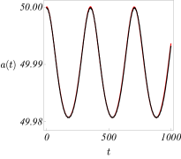
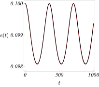
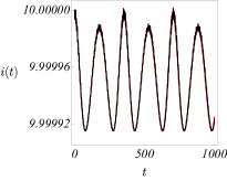
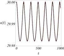
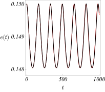
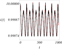
Figure 2: First and second example (ER3BP). Data: $a_{*}=50$AU, $e_{*}=0.1$ ($\nu=3$), $i(0)=10^{\circ}$, $k_{\mu}=k_{\text{mp}}=2$ (top panels); $a_{*}=30$AU, $e_{*}=0.15$ ($\nu=4$), $i(0)=10^{\circ}$, $k_{\mu}=k_{\text{mp}}=2$ (bottom panels). Black curves represent semi-analytic time variations (our method), while red curves stand for Cartesian series.

Fig. 2 shows the comparison between the Cartesian and the semi-analytical propagation of the elements in ‘easy’ cases, where the particle departs from initial conditions $a(0)=50$AU (top left panel) or $a(0)=30$AU (bottom left panel), with a relatively low value of the eccentricity $e(0)=0.1$ or $e(0)=0.15$ respectively (middle panels) and inclination $i(0)=10^{\circ}$ (right panels). In these cases, the distance ratio $\left\lVert r_{1}\right\rVert/\left\lVert R\right\rVert$ is small (about $0.1$-$0.2$), a fact implying that the quadrupolar expansion ($k_{\text{mp}}=2$) suffices to have obtained a relative error of about $0.1\%$ in the representation of the Hamiltonian perturbation $\mathcal{H}_{1}$. Going to higher multipoles is straightforward, albeit with a significant computational cost as the number of terms in the Hamiltonian grows significantly. On the other hand, even with low-order truncations of the Hamiltonian we achieve to have an accurate semi-analytical representation of the $\mathcal{O}(\mu)$ short-period oscillations in all three ‘action-like’ elements (semi-major axis, eccentricity, inclination). Most notably, keeping $a(0)=50$AU but changing the eccentricity to $e(0)=0.7$, i.e., beyond the Laplace value, yields an orbit whose pericenter is at $\left\lVert R_{p}\right\rVert=15$AU, implying a distance ratio $\left\lVert r_{1}\right\rVert/\left\lVert R\right\rVert\approx 0.3$ (Fig. 3). This time, an octupole truncation ($k_{\text{mp}}=3$) is required to produce an approximation of the Hamiltonian model at the level of a relative error of $0.1\%$. Still, however, as shown in Fig. 3 the semi-analytical propagation of the orbit is able to track the fully numerical one with an error which does not exceed $0.2\%$ even close to the orbit’s pericentric passages.

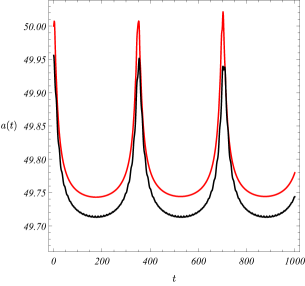
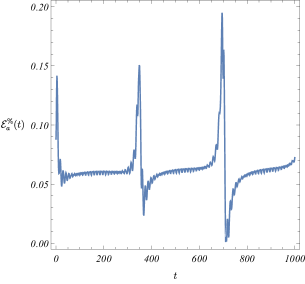
Figure 3: Third example (ER3BP). Data: $a_{*}=50$AU, $e_{*}=0.7$ ($\nu=20$), $i(0)=20^{\circ}$, $k_{\mu}=2$, $k_{\text{mp}}=3$. On the left, the black curve represents the semi-analytic time variation of the semi-major axis (our method) versus the one found by propagation of the Cartesian equations of motion (red). The right panel shows the evolution of the corresponding percent relative error $\mathcal{E}^{\%}_{a}$.

In the above examples, the maximum number of normalization steps at which the secular Hamiltonian is computed was set equal to $j_{max}=3$, $j_{max}=4$ and $j_{max}=4$ respectively, which corresponds to the best match in all cases. As discussed in the next subsection, an estimate of the minimum possible error in the semi-analytic propagation of the trajectories requires computing first the so-called optimal number of normalizations $j_{opt}$ (or equivalently optimal normalization order $\nu+j_{opt}-1$) as a function of the reference values $(a_{*},e_{*})$ within a model given by a preset fixed multipole truncation order. Owing to the fact that the same divisors appear in the ER3BP and in the CR3BP, we verify with numerical examples that the error analysis yields essentially identical results in either case. However, the computation of the optimal normalization is easier to perform in the CR3BP, owing to the considerably smaller number of terms produced in the CAS computation of the normal form. Hence, we now turn our attention to this latter computation.

3.3 Numerical examples in the Sun-Jupiter planar CR3BP: order and size of the optimal remainder

3.3.1 Trajectory propagation: optimal remainder

A considerable reduction of the computational cost occurs in the case of the planar and circular R3BP. This is due, in particular, to the following:

• the dependence on $M_{1}$ becomes explicit ($M_{1}=E_{1}$ in (2)), while $a_{1}=\left\lVert r_{1}\right\rVert$. As a consequence, $\phi_{1}=0$.

• no terms involving $(h,H)$ appear in the disturbing function, thus $\iota_{c},\iota_{s}$ are discarded;

• no terms requiring a book-keeping in terms of the exponent $\nu_{1}$ appear, hence, only $\nu$ is defined, as in (7);

• $d^{\prime(j)}_{l,\lambda,p}=0$ for every $j,l,\lambda,p$ in (89), (85), and consequently $p_{1}=p_{2}\equiv 0$ in (87). This is due to the fact that the expression (16) reduces to

  $$r_{1}\cdot R=\left\lVert r_{1}\right\rVert\left\lVert R\right\rVert\cos(f+g-M_{1})\;,$$ (106)

  which always depends on the difference $g-M_{1}$ by D’Alembert rules. This implies that, unlike the ER3BP, the action $G$ (and the corresponding eccentricity $e$) are integrals of the secular Hamiltonian;

• as a consequence no lower or equal book-keeping order terms appear in any Poisson bracket of the first normalization step in the case $\nu=1$. Hence Proposition 3 is redundant.

Owing to the above, in the planar CR3BP we are able to make normal form computations in a grid of points in the plane $(a_{*},e_{*})$ up to a sufficiently high normalization order so that the asymptotic character of the series computed by the algorithm of Section 2 can show up. To this end, we introduce an estimate of the size of the series’ remainder after $j$ normalization steps via the upper norm bound

$$\mathscr{E}^{(j)}=\sum_{l=\nu+j}^{\nu k_{\mu}}\sum_{s\in\mathbb{Z}^{3}}|d^{(j)}_{l,s}|\geq\left\lVert\mathscr{R}^{(j)}_{\nu+j}\right\rVert_{\infty}\;,\quad j=1,\ldots,\nu(k_{\mu}-1)\;,$$ (107)

where $\left\lVert\cdot\right\rVert_{\infty}$ denotes the sup norm. Plotting $\mathscr{E}^{(j)}$ against the number of normalization steps $j$ allows then to estimate the error committed at any step (size of the remainder). Figure 4 yields an example of such computation. The relevant fact is that there is an optimal number of normalization steps ($j=j_{opt}=6$) where the estimate $\mathscr{E}^{(j)}$ of the remainder size yields a global minimum.

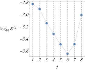
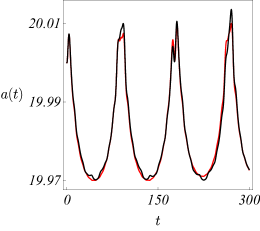
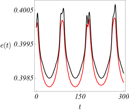
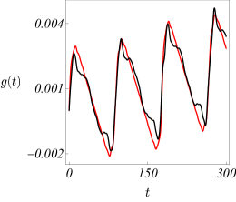
Figure 4: Fourth example (planar CR3BP). Data: $a_{*}=20$AU, $e_{*}=0.4$ ($\nu=8$), $k_{\mu}=2$, $k_{\text{mp}}=3$. The estimate $\mathscr{E}^{(j)}$ is depicted in semi-logarithmic scale on top left panel. The direct comparison of the semi-analytic (black) evolution vs. the fully numerical (red) one for the osculating elements $a(t)$, $e(t)$, $g(t)$ are shown in the top right and bottom panels respectively. The semi-analytic curves are obtained for $j=j_{opt}=6$, where $\mathscr{E}^{(j)}$ is minimum.

Although a systematic investigation of the dependence of the optimal number of normalization steps $j_{opt}$ on the parameters $(a_{*},e_{*})$ is beyond our present scope, Figs. 5 and 6 allow to gain some insight into the question. The most relevant remark concerns the dependence of the behavior of the curve $\mathscr{E}^{(j)}$ (versus $j$) on how close to the ‘hierarchical’ regime the trajectory with reference values $(a_{*},e_{*})$ is. As a measure of the hierarchical character of an orbit we adopt either the ratio of the semi-major axes $a_{1}/a_{*}$, or of the pericentric distances $\left\lVert r_{1}\right\rVert/\left\lVert R_{p}\right\rVert=a_{1}(1-e_{1})/(a_{*}(1-e_{*}))=a_{1}/(a_{*}(1-e_{*}))$. Fig. 5 ($a_{*}=30$AU, $e_{*}=0.5$) implies a pericentric distance ratio $\left\lVert r_{1}\right\rVert/\left\lVert R_{p}\right\rVert\approx 0.3$ smaller than the one of the example of Fig. 4 ($\left\lVert r_{1}\right\rVert/\left\lVert R_{p}\right\rVert\approx 0.4$). We observe that the optimal number of normalization steps in the former case satisfies $j_{opt}=10$, i.e., it is larger than in the latter case. Fig. 6 shows, instead, an example of orbit far from the hierarchical limit, satisfying the estimate $\left\lVert r_{1}\right\rVert/\left\lVert R_{p}\right\rVert\approx 0.7$. In this case a higher order multipole expansion ($k_{\text{mp}}=5$) is required to obtain a precise truncated Hamiltonian model for this orbit. We note, however, that the normalization procedure performs well, producing a decreasing remainder as a function of $j$ up to the point where it is arrested, i.e. $j=6=\nu(k_{\mu}-1)$. We find numerically that this performance is deteriorated as we gradually approach the condition $\left\lVert r_{1}\right\rVert/\left\lVert R\right\rVert=1$, beyond which the multipole expansion of the Hamiltonian is no longer convergent.

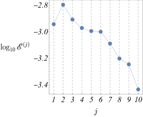
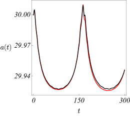
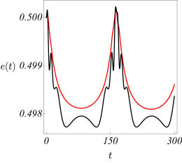
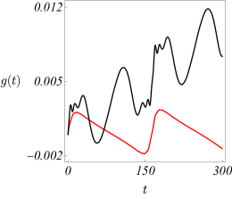
Figure 5: Fifth example (planar CR3BP): $a_{*}=30$AU, $e_{*}=0.5$ ($\nu=10$), $k_{\mu}=2$, $k_{\text{mp}}=3$. Plot types and color conventions are the same as in Fig. 4. The semi-analytic curves are obtained for $j=j_{opt}=10$.

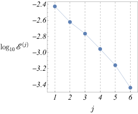
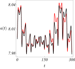
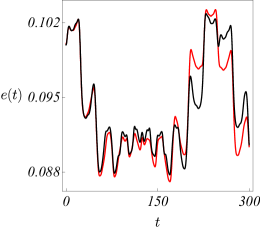
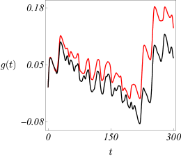
Figure 6: Sixth example (planar CR3BP): $a_{*}=8$, $e_{*}=0.1$ ($\nu=3$), $k_{\mu}=3$, $k_{\text{mp}}=5$. Plot types and color conventions are the same as in Fig. 4. The semi-analytic curves are obtained for $j=j_{opt}=6$.

3.3.2 Semi-analytical determination of the domain of secular motions

The results shown in the two previous subsections refer to isolated examples of orbits treated within various multipole truncation orders as well as different choices of the number of normalization steps, searching each time to arrive at the best approximating secular model given computational restrictions. In the present subsection, we aim to investigate the behavior of the remainder in a closed-form normalization with uniform choice of all truncation orders of the problem, but performed, instead, in a fine grid ($100\times 20$) of reference values in the plane $(a_{*},e_{*})$. To this end, we set $k_{\mu}=2$ (second order in the mass parameter), and fix $k_{\text{mp}}=3$ (octupole approximation). The latter choice, imposed by computational restrictions, yields an initial model whose error with respect to the full Hamiltonian becomes of the order of $1\%$ only for $a_{*}>2a_{1}$. However, for reasons explained below, a computation within the framework of the octupole approximation becomes relevant to the problem addressed in the sequel also in the range $1.5a_{1}<a_{*}<2a_{1}$, while higher multipoles are required to address still smaller values of $a_{*}$.

The result of the above computation is summarized in Fig. 7: the left panel shows in logarithmic color scale the size of the remainder, estimated by the value of $\mathscr{E}^{(n)}(a_{*},e_{*})$ computed as in (107), corresponding to each point in the plane $(a_{*},e_{*})$, where the number of normalization steps is set as $n=\min\{\nu(k_{\mu}-1),7\}=\min\{\nu,7\}$. The maximum value $n=7$ is, again, imposed by computational restrictions, and it implies that $n$ varies with $e_{*}$ up to about $e_{*}=0.37$.

The relevant information in Fig. 7 is provided by the black curve, which corresponds to the isocontour $\mathscr{E}^{(n)}(a_{*},e_{*})=10^{-2}$. Since in the original Hamiltonian we have the estimate $\mathscr{E}^{(0)}(a,e)\coloneqq\mathcal{H}_{1}^{\leq k_{\mu},k_{\text{mp}}}=\mathcal{O}(10^{-2})$, the black curve provides a rough estimate of the limiting border dividing the plane $(a_{*},e_{*})$ in two domains: in the one below the black curve the progressive elimination of the fast angles by the iterative normalization steps leads to a secular model whose remainder decreases with the number of normalization steps $j$ at least up to $j=n$.

A physical interpretation of the border approximated through the isocontour $\mathscr{E}^{(n)}(a_{*},e_{*})=10^{-2}$ can be given through a comparison with a numerical stability map obtained, e.g., as in the right panel of Fig. 7. For each trajectory in a $300\times 900$ grid in $(a,e)$, the plot shows in color scale the value of the Fast Lyapunov Indicator (FLI, see [9] for a review) obtained after integrating the variational equations of motion together with the equations of motion of the full Hamiltonian model for a time equal to $50$ periods of Jupiter. Thus, deep blue colors indicate the most regular, and light yellow the most chaotic orbits as identified by the value of the FLI. Superposed to the FLI cartography are three curves:

1. the ‘perihelion crossing curve’ (red) yields the locus of values satisfying the condition $a(1-e)=\left\lVert r_{J}\right\rVert=a_{J}$ (in the circular case), that is the points where the pericenter of the test particle’s orbit comes at distance equal to the radius of Jupiter’s orbit;

2. the Hill limit [12] (brown) is based on the relationship $C_{\text{Jac}}(a,e)=C_{\text{Jac}}(\mathscr{L}_{1})$, where $C_{\text{Jac}}$ is the particle’s Jacobi constant as function of the orbital elements and $C_{\text{Jac}}(\mathscr{L}_{1})$ its value at the Lagrangian point $\mathscr{L}_{1}$;

3. the isocontour $\mathscr{E}^{(n)}(a,e)=10^{-2}$ (black, same as in the left panel of Fig. 7).

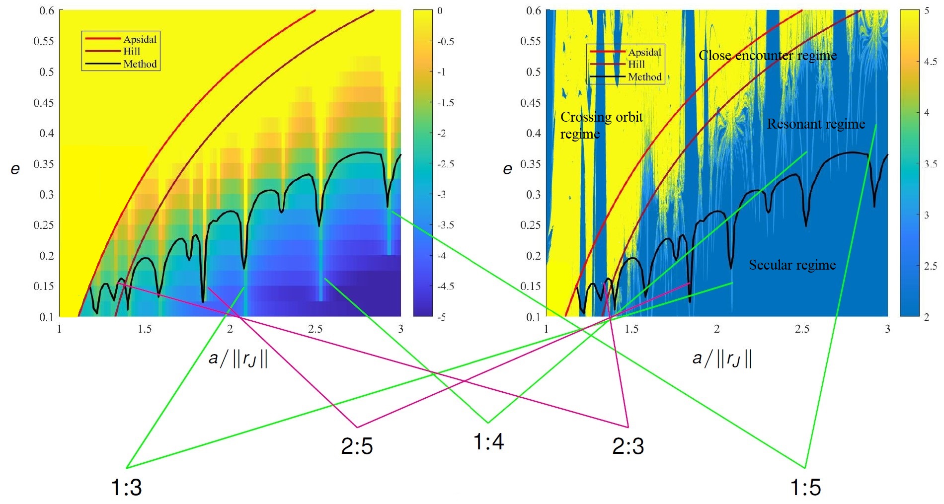
Figure 7: Left panel: computation of $\log_{10}(\mathscr{E}^{(n)})$, $n=\min\{\nu,7\}$, $k_{\text{mp}}=3$, over a $100\times 20$ $(a,e)$ grid. For every $e=e_{*}$, $n$ different normalizations are executed and then evaluated for each $a=a_{*}$. Right panel: short-period FLI map over a $300\times 900$ $(a,e)$ grid of initial data integrated for $50T_{1}$. As indicated, the three curves represent, respectively, the line of constant pericenter of the particle’s trajectory equal to the radius of Jupiter’s orbit $\left\lVert r_{1}\right\rVert=\left\lVert r_{J}\right\rVert$ (red), Hill’s stability criterion (brown) and the isolevel $\mathscr{E}^{(n)}=1\%$ (black). Each region enclosed by two consecutive above curves is labeled with the corresponding regime of motion. The main mean-motion resonances are reported below the pictures.

Of the above three curves, the perihelion crossing curve is analogous, in the R3BP, of the so-called Angular Momentum Deficit criterion (AMD, [8]) used to separate systems protected from perihelia crossings in the case of the full planetary three-body problem. As indicated by the FLI cartography data, Hill’s curve gives an overall better approximation separating the domain of strong chaos (yellow) from the domain of regular or weakly-chaotic orbits (all blue nuances). This is expected, since the Hill’s curve separates orbits for which Jupiter’s gravitational effect becomes (at least temporarily) dominant from those for which it does not. Nevertheless, through the FLI cartography we note the presence of a large domain between the curves (ii) and (iii), where the trajectories, while protected from close encounters, are subject to the long term effects on dynamics produced by resonant multiplets associated with the mean-motion resonances of the problem (the most important of which are marked in the figure). Note that in the octupole approximation, the Hamiltonian contains harmonics including all combinations of the fast angles of the form $\cos(s_{1}f+s_{2}(g-M_{1}))$, with

$$(s_{1},s_{2})=(1,3),(2,3),(3,3),(4,3),(5,3),(6,3),(7,3),$$

$$(1,2),(2,2),(3,2),(4,2),(5,2),(1,1),(2,1),(3,1),(4,1),(5,1),$$

$$(1,-1),(2,-1),(3,-1),(1,-2),(1,-3),$$

thus including all harmonics associated with the mean-motion resonances detected in the FLI cartography of Fig. 7 for $a>1.5a_{J}$. Through the closed-form normalization (Eqs.(69) and (85)) we then obtain small divisors in the series at every value of the semi-major axis $a_{*}$ for which one of the resonant combinations $s_{1}n_{*}-s_{2}n_{J}$, $n_{J}=n_{1}$, takes a value near zero. All these incidences lead to Arnold tongue-like spikes pointing downwards in the curve (iii), marking the failure of the approximation of the orbits based on a non-resonant normal form construction. On the other hand, we observe that, for any value of $a_{*}$ there is a threshold value of the eccentricity $e_{*,s}$, such that, for $e_{*}<e_{*,s}$ no visible effects of the harmonics associated with mean-motion resonances are visible in the FLI cartography. This implies that the secular models constructed by eliminating all harmonics involving the fast angles of the problem describe with good precision the dynamics in this domain, called, for this reason, the domain of secular motions. In physical terms, the domain of secular motions corresponds to initial conditions for which the gravitational perturbation of Jupiter is only felt in the ‘Laplacian’ meaning, i.e., as a mass distributed along a ring coinciding with Jupiter’s orbit. The curve (iii) then yields the limit of this domain, which, as found by the FLI cartography, is well distinct from the limit of the Hill domain.
The overall situation can therefore be summarized with the identification of four regimes of motion (specified in the FLI chart):

• the ‘crossing orbit regime’ (above curve (i));

• the ‘close encounter regime’ (between curves (i) and (ii));

• the ‘resonant regime’ (between curves (ii) and (iii));

• the ‘secular regime’ (below curve (iii)).

4 Conclusions

In summary, in the present paper we have proposed a closed-form method for the derivation of secular Hamiltonian models (normal forms) with a small (albeit finite minimum) remainder applicable to the R3BP in the case when the particle’s trajectory is exterior to the trajectory of the primary perturber. Also, using this method we were led to the definition of a new heuristic limit separating the motions whose character is ‘secular’, i.e., not affected by short-period effects, from the rest of motions in the R3BP. In particular:

1. Section 2 develops the formal aspects of the method, which heavily relies on the use of a book-keeping parameter to simultaneously account for all small quantities of the problem as they appear not only in the Hamiltonian and Lie generating functions, but also in the closed-form version of all formulas involved in the Poisson algebra between the Delaunay canonical variables of the problem. A rigorous demonstration of the consistency of the method is then given through Propositions 1, 2 and 3, which also estabilish the explicit formulas for the implementation of one iterative step of the closed-form normalization algorithm.

2. Section 3 gives numerical examples of the implementation and precision of the algorithm in the spatial elliptic, as well as in the planar circular R3BP, examining, also numerically, the method’s convergence properties. The effect of choosing different truncation orders (in powers of the mass parameter $\mu$ or in the multipole expansion) is discussed, along with several simplifications to the normalization procedure which hold in the circular case. The essentially asymptotic character of the series is established through numerical examples, showing the existence of an optimal number of normalization steps, after which the size of the remainder becomes the minimum possible.

3. A key aspect of the above presented method lies in the possibility to exploit the behavior of the size of the remainder as a function of the number of normalizing steps in order to obtain a clear separation of two well-distinct domains, as also identified by purely numerical (FLI cartography) means: one, called the domain of secular motions corresponds to the domain where the harmonics in the Hamiltonian associated with resonant combinations of the fast angles (anomalies) of the problem produce no dynamical effect on the orbits visible at the level of the FLI cartography. From the semi-analytical point of view, this turns to be the domain where a non-resonant construction as the one proposed in section 2 produces no (nearly-)resonant divisors up to the optimal normalization step. As a consequence, only the angles associated with the motions of the perihelion and of the line of nodes survive in the final normal form. We show numerically how to use the information on the size of the normal form remainder in order to determine semi-analytically the border of the domain of secular motions in the case of the Sun-Jupiter system. We finally give evidence that this border is well distinct from the border of the domains defined either by the Hill stability or by the perihelion crossing criterion.

Appendix

Appendix A Computation of Poisson bracket’s intermediate derivatives

Derivatives (31)–(42) are computed combining adequately definitions (1), the polar relationship (15), including its alternative expression involving the eccentric anomaly $E$

$$\left\lVert R\right\rVert=a(1-e\cos E)\;,$$ (108)

$\left\lVert r_{1}\right\rVert$ via (2) (analogous to (108)), Kepler’s equations

$$\ell=E-e\sin E\;,\quad\quad M_{1}=E_{1}-e_{1}\sin E_{1}\;,$$ (109)

and the trigonometric equalities

$$\cos f=\frac{\cos E-e}{1-e\cos E}\;,\quad\quad\sin f=\frac{\eta\sin E}{1-e\cos E}\;.$$ (110)

Eq.(31) comes from (108) and (15) by total differentiation with respect to $\ell$:

$$\frac{\text{d}}{\text{d}\ell}\left\lVert R\right\rVert\stackrel{{\scriptstyle\text{\eqref{eqn:normRE}}}}{{=}}\frac{\partial\left\lVert R\right\rVert}{\partial E}\frac{\partial E}{\partial\ell}=\frac{ae\sin E}{1-e\cos E}\stackrel{{\scriptstyle\text{\eqref{eqn:normR}}}}{{=}}\frac{\partial\left\lVert R\right\rVert}{\partial f}\frac{\partial f}{\partial\ell}=\frac{a\eta^{2}e\sin f}{(1+e\cos f)^{2}}\frac{\partial f}{\partial\ell}\;,$$

since $a$, $e$ do not depend on $\ell$, where $\partial E/\partial\ell$ is deduced from the first of (109) making use of the derivative of inverse functions ($\partial\ell/\partial E\neq 0$ is ensured). Thus the result by (110).
Eqs.(32), (33) are straightforwardly yielded taking respectively ordinary differentiation and the inverse derivative once again of $\text{d}M_{1}/\text{d}E_{1}\neq 0$ from the second of (109):

$$\frac{\text{d}E_{1}}{\text{d}M_{1}}=\frac{1}{1-e_{1}\cos E_{1}}=\frac{a_{1}}{\left\lVert r_{1}\right\rVert}\;.$$

Now solving for $e$ in (1) and partially differentiating, we immediately have Eqs.(35) and (37), from which Eqs.(36), (38) as

$$\frac{\partial\eta}{\partial\delta L}=-\frac{e}{\eta}\frac{\partial e}{\partial\delta L}=-\frac{\eta}{L}\;,\quad\quad\frac{\partial\eta}{\partial G}=-\frac{e}{\eta}\frac{\partial e}{\partial G}=\frac{1}{L}\;.$$

The true anomaly derivatives with respect to the actions are slightly more elaborated. Employing (110),

$$-\sin f\frac{\partial f}{\partial\delta L}=\frac{\partial}{\partial\delta L}\cos f=\frac{\partial}{\partial e}\left(\frac{\cos E-e}{1-e\cos E}\right)\frac{\partial e}{\partial\delta L}+\frac{\partial}{\partial E}\left(\frac{\cos E-e}{1-e\cos E}\right)\frac{\partial E}{\partial\delta L}\;,$$

that leads upon simplifications to

$$\frac{\partial f}{\partial\delta L}=\frac{\sin f}{eL}+\frac{1+e\cos f}{\eta}\frac{\partial E}{\partial\delta L}\;;$$

finally we explicit $\partial E/\partial\delta L$ exploiting the corresponding Kepler equation (109) and the inter-independence $\ell,\delta L$ by conjugacy:

$$0=\frac{\text{d}}{\text{d}\delta L}(E-e\sin E)=\frac{\partial E}{\partial\delta L}-\frac{\partial e}{\partial\delta L}\sin E-e\cos E\frac{\partial E}{\partial\delta L}\;\implies\;\frac{\partial E}{\partial\delta L}=\frac{\eta\sin f}{eL}\;,$$

thereby Eq.(34).
The relation for $\partial f/\partial G$ is achieved precisely in the same manner, so one finds out

$$\frac{\partial f}{\partial G}=-\frac{\sin f}{\eta eL}+\frac{1+e\cos f}{\eta}\frac{\partial E}{\partial G}\;,\quad\quad\frac{\partial E}{\partial G}=-\frac{\sin f}{eL}\;,$$

that is Eq.(2.3.1).
Finally, derivatives (39), (41) involving $\iota_{c}=\cos i$ easily follow again by partial differentiation in (1) with respect to $G$ and $H$ respectively; while for those containing $\iota_{s}=\sin i$ we can rely, for example, to the identity $\sin^{2}i+\cos^{2}i=1$:

$$0=2\sin i\frac{\partial\iota_{s}}{\partial G}+2\cos i\frac{\partial\iota_{c}}{\partial G}\;$$

and consequently Eq.(40) provided $\sin i\neq 0$, as well as Eq.(42) repeating the same argument with the variable $H$.

Appendix B Example of normalization for a $\boldsymbol{\mu^{2}}$ quadrupolar expansion

Consider the following toy model Hamiltonian with $k_{\mu}=k_{\text{mp}}=\nu=2$, $\nu_{1}=1$, according to conventions introduced in §2.4.1:

$$\mathscr{H}^{(0)}=\mathscr{Z}_{0}+\mathscr{R}_{2,2}^{(0)}+\mathscr{R}_{2,3}^{(0)}+\mathscr{R}_{2,4}^{(0)}\;,$$

where

$$\mathscr{R}^{(0)}_{2,2}=\sigma^{2}\Bigg{(}-\frac{3a_{1}^{3}\mathcal{G}^{4}\mu m_{0}^{4}\iota_{c}^{2}\cos\left(2\left(E_{1}-f-g-h\right)\right)}{16L_{*}^{6}\left\lVert r_{1}\right\rVert}\\ -\frac{3a_{1}^{3}\mathcal{G}^{4}\mu m_{0}^{4}\iota_{c}^{2}\cos\left(2\left(E_{1}+f+g-h\right)\right)}{16L_{*}^{6}\left\lVert r_{1}\right\rVert}-\frac{3a_{1}^{3}\mathcal{G}^{4}\mu m_{0}^{4}\iota_{c}\cos\left(2\left(E_{1}-f-g-h\right)\right)}{8L_{*}^{6}\left\lVert r_{1}\right\rVert}\\ +\frac{3a_{1}^{3}\mathcal{G}^{4}\mu m_{0}^{4}\iota_{c}\cos\left(2\left(E_{1}+f+g-h\right)\right)}{8L_{*}^{6}\left\lVert r_{1}\right\rVert}+\frac{3a_{1}^{3}\mathcal{G}^{4}\mu m_{0}^{4}\iota_{c}^{2}\cos\left(2\left(E_{1}-h\right)\right)}{8L_{*}^{6}\left\lVert r_{1}\right\rVert}\\ +\frac{3a_{1}^{3}\mathcal{G}^{4}\mu m_{0}^{4}\iota_{c}^{2}\cos(2(f+g))}{8L_{*}^{6}\left\lVert r_{1}\right\rVert}-\frac{3a_{1}^{3}\mathcal{G}^{4}\mu m_{0}^{4}\iota_{c}^{2}}{8L_{*}^{6}\left\lVert r_{1}\right\rVert}-\frac{3a_{1}^{3}\mathcal{G}^{4}\mu m_{0}^{4}\cos\left(2\left(E_{1}-f-g-h\right)\right)}{16L_{*}^{6}\left\lVert r_{1}\right\rVert}\\ -\frac{3a_{1}^{3}\mathcal{G}^{4}\mu m_{0}^{4}\cos\left(2\left(E_{1}+f+g-h\right)\right)}{16L_{*}^{6}\left\lVert r_{1}\right\rVert}-\frac{3a_{1}^{3}\mathcal{G}^{4}\mu m_{0}^{4}\cos\left(2\left(E_{1}-h\right)\right)}{8L_{*}^{6}\left\lVert r_{1}\right\rVert}\\ -\frac{3a_{1}^{3}\mathcal{G}^{4}\mu m_{0}^{4}\cos(2(f+g))}{8L_{*}^{6}\left\lVert r_{1}\right\rVert}+\frac{a_{1}^{3}\mathcal{G}^{4}\mu m_{0}^{4}}{8L_{*}^{6}\left\lVert r_{1}\right\rVert}-\frac{3a_{1}\delta L^{2}\mathcal{G}^{2}m_{0}^{2}}{2L_{*}^{4}\left\lVert r_{1}\right\rVert}-\frac{a_{1}\mathcal{G}^{2}\mu m_{0}^{2}}{L_{*}^{2}\left\lVert r_{1}\right\rVert}\Bigg{)}\;.$$

The first step $j=1$ of the method aims precisely at normalizing $\mathscr{R}_{2,2}^{(0)}$ via (70) solved by

$$\chi_{2}^{(1)}=\sigma^{3}\Bigg{(}\frac{3\mathcal{G}^{4}\mu a_{1}^{2}\iota_{c}^{2}\phi_{1}n_{*}^{2}m_{0}^{4}}{8n_{1}L_{*}^{6}\left(n_{1}^{2}-n_{*}^{2}\right)}-\frac{\mathcal{G}^{4}\mu a_{1}^{2}\phi_{1}n_{*}^{2}m_{0}^{4}}{8n_{1}L_{*}^{6}\left(n_{1}^{2}-n_{*}^{2}\right)}\\ -\frac{3\mathcal{G}^{4}\mu a_{1}^{2}n_{1}\iota_{c}^{2}\phi_{1}m_{0}^{4}}{8L_{*}^{6}\left(n_{1}^{2}-n_{*}^{2}\right)}+\frac{\mathcal{G}^{4}\mu a_{1}^{2}n_{1}\phi_{1}m_{0}^{4}}{8L_{*}^{6}\left(n_{1}^{2}-n_{*}^{2}\right)}+\frac{\mathcal{G}^{2}\mu\phi_{1}n_{*}^{2}m_{0}^{2}}{n_{1}L_{*}^{2}\left(n_{1}^{2}-n_{*}^{2}\right)}\\ +\frac{3\mathcal{G}^{2}\delta L^{2}\phi_{1}n_{*}^{2}m_{0}^{2}}{2n_{1}L_{*}^{4}\left(n_{1}^{2}-n_{*}^{2}\right)}-\frac{\mathcal{G}^{2}\mu n_{1}\phi_{1}m_{0}^{2}}{L_{*}^{2}\left(n_{1}^{2}-n_{*}^{2}\right)}-\frac{3\mathcal{G}^{2}\delta L^{2}n_{1}\phi_{1}m_{0}^{2}}{2L_{*}^{4}\left(n_{1}^{2}-n_{*}^{2}\right)}\Bigg{)}\\ +\sigma^{2}\Bigg{(}-\frac{3\mathcal{G}^{4}\mu\sin\left(2\left(E_{1}-h\right)\right)a_{1}^{2}\iota_{c}^{2}n_{*}^{2}m_{0}^{4}}{16n_{1}L_{*}^{6}\left(n_{1}^{2}-n_{*}^{2}\right)}+\frac{3\mathcal{G}^{4}\mu\sin\left(2\left(E_{1}-h\right)\right)a_{1}^{2}n_{*}^{2}m_{0}^{4}}{16n_{1}L_{*}^{6}\left(n_{1}^{2}-n_{*}^{2}\right)}\\ +\frac{3\mathcal{G}^{4}\mu\sin(2(f+g))a_{1}^{2}n_{*}m_{0}^{4}}{16L_{*}^{6}\left(n_{1}^{2}-n_{*}^{2}\right)}-\frac{3\mathcal{G}^{4}\mu\sin\left(2\left(-f-g-h+E_{1}\right)\right)a_{1}^{2}n_{*}m_{0}^{4}}{32L_{*}^{6}\left(n_{1}^{2}-n_{*}^{2}\right)}\\ +\frac{3\mathcal{G}^{4}\mu\sin\left(2\left(f+g-h+E_{1}\right)\right)a_{1}^{2}n_{*}m_{0}^{4}}{32L_{*}^{6}\left(n_{1}^{2}-n_{*}^{2}\right)}-\frac{3\mathcal{G}^{4}\mu\sin(2(f+g))a_{1}^{2}\iota_{c}^{2}n_{*}m_{0}^{4}}{16L_{*}^{6}\left(n_{1}^{2}-n_{*}^{2}\right)}\\ -\frac{3\mathcal{G}^{4}\mu\sin\left(2\left(-f-g-h+E_{1}\right)\right)a_{1}^{2}\iota_{c}^{2}n_{*}m_{0}^{4}}{32L_{*}^{6}\left(n_{1}^{2}-n_{*}^{2}\right)}+\frac{3\mathcal{G}^{4}\mu\sin\left(2\left(f+g-h+E_{1}\right)\right)a_{1}^{2}\iota_{c}^{2}n_{*}m_{0}^{4}}{32L_{*}^{6}\left(n_{1}^{2}-n_{*}^{2}\right)}\\ -\frac{3\mathcal{G}^{4}\mu\sin\left(2\left(-f-g-h+E_{1}\right)\right)a_{1}^{2}\iota_{c}n_{*}m_{0}^{4}}{16L_{*}^{6}\left(n_{1}^{2}-n_{*}^{2}\right)}-\frac{3\mathcal{G}^{4}\mu\sin\left(2\left(f+g-h+E_{1}\right)\right)a_{1}^{2}\iota_{c}n_{*}m_{0}^{4}}{16L_{*}^{6}\left(n_{1}^{2}-n_{*}^{2}\right)}\\ +\frac{3\mathcal{G}^{4}\mu\sin\left(2\left(E_{1}-h\right)\right)a_{1}^{2}n_{1}\iota_{c}^{2}m_{0}^{4}}{16L_{*}^{6}\left(n_{1}^{2}-n_{*}^{2}\right)}-\frac{3\mathcal{G}^{4}\mu\sin\left(2\left(-f-g-h+E_{1}\right)\right)a_{1}^{2}n_{1}\iota_{c}^{2}m_{0}^{4}}{32L_{*}^{6}\left(n_{1}^{2}-n_{*}^{2}\right)}\\ -\frac{3\mathcal{G}^{4}\mu\sin\left(2\left(f+g-h+E_{1}\right)\right)a_{1}^{2}n_{1}\iota_{c}^{2}m_{0}^{4}}{32L_{*}^{6}\left(n_{1}^{2}-n_{*}^{2}\right)}-\frac{3\mathcal{G}^{4}\mu\sin\left(2\left(E_{1}-h\right)\right)a_{1}^{2}n_{1}m_{0}^{4}}{16L_{*}^{6}\left(n_{1}^{2}-n_{*}^{2}\right)}\\ -\frac{3\mathcal{G}^{4}\mu\sin\left(2\left(-f-g-h+E_{1}\right)\right)a_{1}^{2}n_{1}m_{0}^{4}}{32L_{*}^{6}\left(n_{1}^{2}-n_{*}^{2}\right)}-\frac{3\mathcal{G}^{4}\mu\sin\left(2\left(f+g-h+E_{1}\right)\right)a_{1}^{2}n_{1}m_{0}^{4}}{32L_{*}^{6}\left(n_{1}^{2}-n_{*}^{2}\right)}\\ -\frac{3\mathcal{G}^{4}\mu\sin\left(2\left(-f-g-h+E_{1}\right)\right)a_{1}^{2}n_{1}\iota_{c}m_{0}^{4}}{16L_{*}^{6}\left(n_{1}^{2}-n_{*}^{2}\right)}+\frac{3\mathcal{G}^{4}\mu\sin\left(2\left(f+g-h+E_{1}\right)\right)a_{1}^{2}n_{1}\iota_{c}m_{0}^{4}}{16L_{*}^{6}\left(n_{1}^{2}-n_{*}^{2}\right)}\\ -\frac{3\mathcal{G}^{4}\mu\sin(2(f+g))a_{1}^{2}n_{1}^{2}m_{0}^{4}}{16L_{*}^{6}n_{*}\left(n_{1}^{2}-n_{*}^{2}\right)}+\frac{3\mathcal{G}^{4}\mu\sin(2(f+g))a_{1}^{2}n_{1}^{2}\iota_{c}^{2}m_{0}^{4}}{16L_{*}^{6}n_{*}\left(n_{1}^{2}-n_{*}^{2}\right)}\Bigg{)}\;,$$

so that the new truncated Hamiltonian becomes

$$\mathscr{H}^{(1)}=\mathscr{Z}_{0}+\mathscr{Z}^{(1)}_{2}+\mathscr{R}^{(1)}_{3,3}+\mathscr{R}^{(1)}_{3,4}\;,$$

with

$$\mathscr{Z}_{2}^{(1)}=\sigma^{2}\left(-\frac{3a_{1}^{2}\mathcal{G}^{4}\mu m_{0}^{4}\iota_{c}^{2}}{8L_{*}^{6}}+\frac{a_{1}^{2}\mathcal{G}^{4}\mu m_{0}^{4}}{8L_{*}^{6}}-\frac{3\delta L^{2}\mathcal{G}^{2}m_{0}^{2}}{2L_{*}^{4}}-\frac{\mathcal{G}^{2}\mu m_{0}^{2}}{L_{*}^{2}}\right)$$

and

$$\mathscr{R}^{(1)}_{3,3}=\sigma^{3}\Bigg{(}-\frac{3e\mathcal{G}^{4}\mu\cos\left(f+2g+2h-2E_{1}\right)a_{1}^{3}\iota_{c}^{2}n_{*}m_{0}^{4}}{8\eta^{3}\left\lVert r_{1}\right\rVert L_{*}^{6}\left(2n_{1}-2n_{*}\right)}\\ -\frac{3e\mathcal{G}^{4}\mu\cos\left(3f+2g+2h-2E_{1}\right)a_{1}^{3}\iota_{c}^{2}n_{*}m_{0}^{4}}{8\eta^{3}\left\lVert r_{1}\right\rVert L_{*}^{6}\left(2n_{1}-2n_{*}\right)}+\frac{3\mathcal{G}^{4}\mu\cos\left(2f+2g+2h-3E_{1}\right)a_{1}^{3}e_{1}\iota_{c}^{2}n_{*}m_{0}^{4}}{16\left\lVert r_{1}\right\rVert L_{*}^{6}\left(2n_{1}-2n_{*}\right)}\\ +\frac{3\mathcal{G}^{4}\mu\cos\left(2f+2g+2h-E_{1}\right)a_{1}^{3}e_{1}\iota_{c}^{2}n_{*}m_{0}^{4}}{16\left\lVert r_{1}\right\rVert L_{*}^{6}\left(2n_{1}-2n_{*}\right)}-\frac{3e\mathcal{G}^{4}\mu\cos\left(f+2g+2h-2E_{1}\right)a_{1}^{3}\iota_{c}n_{*}m_{0}^{4}}{4\eta^{3}\left\lVert r_{1}\right\rVert L_{*}^{6}\left(2n_{1}-2n_{*}\right)}\\ -\frac{3e\mathcal{G}^{4}\mu\cos\left(3f+2g+2h-2E_{1}\right)a_{1}^{3}\iota_{c}n_{*}m_{0}^{4}}{4\eta^{3}\left\lVert r_{1}\right\rVert L_{*}^{6}\left(2n_{1}-2n_{*}\right)}+\frac{3\mathcal{G}^{4}\mu\cos\left(2f+2g+2h-3E_{1}\right)a_{1}^{3}e_{1}\iota_{c}n_{*}m_{0}^{4}}{8\left\lVert r_{1}\right\rVert L_{*}^{6}\left(2n_{1}-2n_{*}\right)}\\ +\frac{3\mathcal{G}^{4}\mu\cos\left(2f+2g+2h-E_{1}\right)a_{1}^{3}e_{1}\iota_{c}n_{*}m_{0}^{4}}{8\left\lVert r_{1}\right\rVert L_{*}^{6}\left(2n_{1}-2n_{*}\right)}-\frac{3e\mathcal{G}^{4}\mu\cos\left(f+2g+2h-2E_{1}\right)a_{1}^{3}n_{*}m_{0}^{4}}{8\eta^{3}\left\lVert r_{1}\right\rVert L_{*}^{6}\left(2n_{1}-2n_{*}\right)}\\ -\frac{3e\mathcal{G}^{4}\mu\cos\left(3f+2g+2h-2E_{1}\right)a_{1}^{3}n_{*}m_{0}^{4}}{8\eta^{3}\left\lVert r_{1}\right\rVert L_{*}^{6}\left(2n_{1}-2n_{*}\right)}+\frac{3\mathcal{G}^{4}\mu\cos\left(2f+2g+2h-3E_{1}\right)a_{1}^{3}e_{1}n_{*}m_{0}^{4}}{16\left\lVert r_{1}\right\rVert L_{*}^{6}\left(2n_{1}-2n_{*}\right)}\\ +\frac{3\mathcal{G}^{4}\mu\cos\left(2f+2g+2h-E_{1}\right)a_{1}^{3}e_{1}n_{*}m_{0}^{4}}{16\left\lVert r_{1}\right\rVert L_{*}^{6}\left(2n_{1}-2n_{*}\right)}+\frac{3e\mathcal{G}^{4}\mu\cos\left(f+2g-2h+2E_{1}\right)a_{1}^{3}\iota_{c}^{2}n_{*}m_{0}^{4}}{8\eta^{3}\left\lVert r_{1}\right\rVert L_{*}^{6}\left(2n_{1}+2n_{*}\right)}\\ +\frac{3e\mathcal{G}^{4}\mu\cos\left(3f+2g-2h+2E_{1}\right)a_{1}^{3}\iota_{c}^{2}n_{*}m_{0}^{4}}{8\eta^{3}\left\lVert r_{1}\right\rVert L_{*}^{6}\left(2n_{1}+2n_{*}\right)}-\frac{3\mathcal{G}^{4}\mu\cos\left(2f+2g-2h+E_{1}\right)a_{1}^{3}e_{1}\iota_{c}^{2}n_{*}m_{0}^{4}}{16\left\lVert r_{1}\right\rVert L_{*}^{6}\left(2n_{1}+2n_{*}\right)}\\ -\frac{3\mathcal{G}^{4}\mu\cos\left(2f+2g-2h+3E_{1}\right)a_{1}^{3}e_{1}\iota_{c}^{2}n_{*}m_{0}^{4}}{16\left\lVert r_{1}\right\rVert L_{*}^{6}\left(2n_{1}+2n_{*}\right)}-\frac{3e\mathcal{G}^{4}\mu\cos\left(f+2g-2h+2E_{1}\right)a_{1}^{3}\iota_{c}n_{*}m_{0}^{4}}{4\eta^{3}\left\lVert r_{1}\right\rVert L_{*}^{6}\left(2n_{1}+2n_{*}\right)}\\ -\frac{3e\mathcal{G}^{4}\mu\cos\left(3f+2g-2h+2E_{1}\right)a_{1}^{3}\iota_{c}n_{*}m_{0}^{4}}{4\eta^{3}\left\lVert r_{1}\right\rVert L_{*}^{6}\left(2n_{1}+2n_{*}\right)}+\frac{3\mathcal{G}^{4}\mu\cos\left(2f+2g-2h+E_{1}\right)a_{1}^{3}e_{1}\iota_{c}n_{*}m_{0}^{4}}{8\left\lVert r_{1}\right\rVert L_{*}^{6}\left(2n_{1}+2n_{*}\right)}\\ +\frac{3\mathcal{G}^{4}\mu\cos\left(2f+2g-2h+3E_{1}\right)a_{1}^{3}e_{1}\iota_{c}n_{*}m_{0}^{4}}{8\left\lVert r_{1}\right\rVert L_{*}^{6}\left(2n_{1}+2n_{*}\right)}+\frac{3e\mathcal{G}^{4}\mu\cos\left(f+2g-2h+2E_{1}\right)a_{1}^{3}n_{*}m_{0}^{4}}{8\eta^{3}\left\lVert r_{1}\right\rVert L_{*}^{6}\left(2n_{1}+2n_{*}\right)}\\ +\frac{3e\mathcal{G}^{4}\mu\cos\left(3f+2g-2h+2E_{1}\right)a_{1}^{3}n_{*}m_{0}^{4}}{8\eta^{3}\left\lVert r_{1}\right\rVert L_{*}^{6}\left(2n_{1}+2n_{*}\right)}-\frac{3\mathcal{G}^{4}\mu\cos\left(2f+2g-2h+E_{1}\right)a_{1}^{3}e_{1}n_{*}m_{0}^{4}}{16\left\lVert r_{1}\right\rVert L_{*}^{6}\left(2n_{1}+2n_{*}\right)}\\ -\frac{3\mathcal{G}^{4}\mu\cos\left(2f+2g-2h+3E_{1}\right)a_{1}^{3}e_{1}n_{*}m_{0}^{4}}{16\left\lVert r_{1}\right\rVert L_{*}^{6}\left(2n_{1}+2n_{*}\right)}-\frac{9e\mathcal{G}^{4}\mu\cos(f)a_{1}^{3}\iota_{c}^{2}m_{0}^{4}}{8\left\lVert r_{1}\right\rVert L_{*}^{6}}\\ +\frac{9e\mathcal{G}^{4}\mu\cos(f+2g)a_{1}^{3}\iota_{c}^{2}m_{0}^{4}}{16\left\lVert r_{1}\right\rVert L_{*}^{6}}-\frac{3e\mathcal{G}^{4}\mu\cos(f+2g)a_{1}^{3}\iota_{c}^{2}m_{0}^{4}}{8\eta^{3}\left\lVert r_{1}\right\rVert L_{*}^{6}}\\ +\frac{9e\mathcal{G}^{4}\mu\cos(3f+2g)a_{1}^{3}\iota_{c}^{2}m_{0}^{4}}{16\left\lVert r_{1}\right\rVert L_{*}^{6}}-\frac{3e\mathcal{G}^{4}\mu\cos(3f+2g)a_{1}^{3}\iota_{c}^{2}m_{0}^{4}}{8\eta^{3}\left\lVert r_{1}\right\rVert L_{*}^{6}}\\ +\frac{9e\mathcal{G}^{4}\mu\cos\left(f+2h-2E_{1}\right)a_{1}^{3}\iota_{c}^{2}m_{0}^{4}}{16\left\lVert r_{1}\right\rVert L_{*}^{6}}-\frac{9e\mathcal{G}^{4}\mu\cos\left(f+2g+2h-2E_{1}\right)a_{1}^{3}\iota_{c}^{2}m_{0}^{4}}{32\left\lVert r_{1}\right\rVert L_{*}^{6}}\\ -\frac{9e\mathcal{G}^{4}\mu\cos\left(3f+2g+2h-2E_{1}\right)a_{1}^{3}\iota_{c}^{2}m_{0}^{4}}{32\left\lVert r_{1}\right\rVert L_{*}^{6}}+\frac{9e\mathcal{G}^{4}\mu\cos\left(f-2h+2E_{1}\right)a_{1}^{3}\iota_{c}^{2}m_{0}^{4}}{16\left\lVert r_{1}\right\rVert L_{*}^{6}}\\ -\frac{9e\mathcal{G}^{4}\mu\cos\left(f+2g-2h+2E_{1}\right)a_{1}^{3}\iota_{c}^{2}m_{0}^{4}}{32\left\lVert r_{1}\right\rVert L_{*}^{6}}-\frac{9e\mathcal{G}^{4}\mu\cos\left(3f+2g-2h+2E_{1}\right)a_{1}^{3}\iota_{c}^{2}m_{0}^{4}}{32\left\lVert r_{1}\right\rVert L_{*}^{6}}\\ \allowdisplaybreaks-\frac{3\mathcal{G}^{4}\mu\cos\left(2h-3E_{1}\right)a_{1}^{3}e_{1}\iota_{c}^{2}m_{0}^{4}}{16\left\lVert r_{1}\right\rVert L_{*}^{6}}+\frac{3\mathcal{G}^{4}\mu\cos\left(2f+2g+2h-3E_{1}\right)a_{1}^{3}e_{1}\iota_{c}^{2}m_{0}^{4}}{32\left\lVert r_{1}\right\rVert L_{*}^{6}}\\ -\frac{3\mathcal{G}^{4}\mu\cos\left(2f+2g-E_{1}\right)a_{1}^{3}e_{1}\iota_{c}^{2}m_{0}^{4}}{8\left\lVert r_{1}\right\rVert L_{*}^{6}}-\frac{15\mathcal{G}^{4}\mu\cos\left(2h-E_{1}\right)a_{1}^{3}e_{1}\iota_{c}^{2}m_{0}^{4}}{16\left\lVert r_{1}\right\rVert L_{*}^{6}}\\ +\frac{15\mathcal{G}^{4}\mu\cos\left(2f+2g+2h-E_{1}\right)a_{1}^{3}e_{1}\iota_{c}^{2}m_{0}^{4}}{32\left\lVert r_{1}\right\rVert L_{*}^{6}}+\frac{9\mathcal{G}^{4}\mu\cos\left(E_{1}\right)a_{1}^{3}e_{1}\iota_{c}^{2}m_{0}^{4}}{8\left\lVert r_{1}\right\rVert L_{*}^{6}}\\ -\frac{3\mathcal{G}^{4}\mu\cos\left(2f+2g+E_{1}\right)a_{1}^{3}e_{1}\iota_{c}^{2}m_{0}^{4}}{8\left\lVert r_{1}\right\rVert L_{*}^{6}}+\frac{15\mathcal{G}^{4}\mu\cos\left(2f+2g-2h+E_{1}\right)a_{1}^{3}e_{1}\iota_{c}^{2}m_{0}^{4}}{32\left\lVert r_{1}\right\rVert L_{*}^{6}}\\ +\frac{3\mathcal{G}^{4}\mu\cos\left(2f+2g-2h+3E_{1}\right)a_{1}^{3}e_{1}\iota_{c}^{2}m_{0}^{4}}{32\left\lVert r_{1}\right\rVert L_{*}^{6}}-\frac{9e\mathcal{G}^{4}\mu\cos\left(f+2g+2h-2E_{1}\right)a_{1}^{3}\iota_{c}m_{0}^{4}}{16\left\lVert r_{1}\right\rVert L_{*}^{6}}\\ -\frac{9e\mathcal{G}^{4}\mu\cos\left(3f+2g+2h-2E_{1}\right)a_{1}^{3}\iota_{c}m_{0}^{4}}{16\left\lVert r_{1}\right\rVert L_{*}^{6}}+\frac{9e\mathcal{G}^{4}\mu\cos\left(f+2g-2h+2E_{1}\right)a_{1}^{3}\iota_{c}m_{0}^{4}}{16\left\lVert r_{1}\right\rVert L_{*}^{6}}\\ +\frac{9e\mathcal{G}^{4}\mu\cos\left(3f+2g-2h+2E_{1}\right)a_{1}^{3}\iota_{c}m_{0}^{4}}{16\left\lVert r_{1}\right\rVert L_{*}^{6}}+\frac{3\mathcal{G}^{4}\mu\cos\left(2f+2g+2h-3E_{1}\right)a_{1}^{3}e_{1}\iota_{c}m_{0}^{4}}{16\left\lVert r_{1}\right\rVert L_{*}^{6}}\\ +\frac{15\mathcal{G}^{4}\mu\cos\left(2f+2g+2h-E_{1}\right)a_{1}^{3}e_{1}\iota_{c}m_{0}^{4}}{16\left\lVert r_{1}\right\rVert L_{*}^{6}}-\frac{15\mathcal{G}^{4}\mu\cos\left(2f+2g-2h+E_{1}\right)a_{1}^{3}e_{1}\iota_{c}m_{0}^{4}}{16\left\lVert r_{1}\right\rVert L_{*}^{6}}\\ -\frac{3\mathcal{G}^{4}\mu\cos\left(2f+2g-2h+3E_{1}\right)a_{1}^{3}e_{1}\iota_{c}m_{0}^{4}}{16\left\lVert r_{1}\right\rVert L_{*}^{6}}+\frac{3e\mathcal{G}^{4}\mu\cos(f)a_{1}^{3}m_{0}^{4}}{8\left\lVert r_{1}\right\rVert L_{*}^{6}}\\ -\frac{9e\mathcal{G}^{4}\mu\cos(f+2g)a_{1}^{3}m_{0}^{4}}{16\left\lVert r_{1}\right\rVert L_{*}^{6}}+\frac{3e\mathcal{G}^{4}\mu\cos(f+2g)a_{1}^{3}m_{0}^{4}}{8\eta^{3}\left\lVert r_{1}\right\rVert L_{*}^{6}}\\ -\frac{9e\mathcal{G}^{4}\mu\cos(3f+2g)a_{1}^{3}m_{0}^{4}}{16\left\lVert r_{1}\right\rVert L_{*}^{6}}+\frac{3e\mathcal{G}^{4}\mu\cos(3f+2g)a_{1}^{3}m_{0}^{4}}{8\eta^{3}\left\lVert r_{1}\right\rVert L_{*}^{6}}\\ -\frac{9e\mathcal{G}^{4}\mu\cos\left(f+2h-2E_{1}\right)a_{1}^{3}m_{0}^{4}}{16\left\lVert r_{1}\right\rVert L_{*}^{6}}-\frac{9e\mathcal{G}^{4}\mu\cos\left(f+2g+2h-2E_{1}\right)a_{1}^{3}m_{0}^{4}}{32\left\lVert r_{1}\right\rVert L_{*}^{6}}\\ -\frac{9e\mathcal{G}^{4}\mu\cos\left(3f+2g+2h-2E_{1}\right)a_{1}^{3}m_{0}^{4}}{32\left\lVert r_{1}\right\rVert L_{*}^{6}}-\frac{9e\mathcal{G}^{4}\mu\cos\left(f-2h+2E_{1}\right)a_{1}^{3}m_{0}^{4}}{16\left\lVert r_{1}\right\rVert L_{*}^{6}}\\ -\frac{9e\mathcal{G}^{4}\mu\cos\left(f+2g-2h+2E_{1}\right)a_{1}^{3}m_{0}^{4}}{32\left\lVert r_{1}\right\rVert L_{*}^{6}}-\frac{9e\mathcal{G}^{4}\mu\cos\left(3f+2g-2h+2E_{1}\right)a_{1}^{3}m_{0}^{4}}{32\left\lVert r_{1}\right\rVert L_{*}^{6}}\\ +\frac{3\mathcal{G}^{4}\mu\cos\left(2h-3E_{1}\right)a_{1}^{3}e_{1}m_{0}^{4}}{16\left\lVert r_{1}\right\rVert L_{*}^{6}}+\frac{3\mathcal{G}^{4}\mu\cos\left(2f+2g+2h-3E_{1}\right)a_{1}^{3}e_{1}m_{0}^{4}}{32\left\lVert r_{1}\right\rVert L_{*}^{6}}\\ +\frac{3\mathcal{G}^{4}\mu\cos\left(2f+2g-E_{1}\right)a_{1}^{3}e_{1}m_{0}^{4}}{8\left\lVert r_{1}\right\rVert L_{*}^{6}}+\frac{15\mathcal{G}^{4}\mu\cos\left(2h-E_{1}\right)a_{1}^{3}e_{1}m_{0}^{4}}{16\left\lVert r_{1}\right\rVert L_{*}^{6}}\\ +\frac{15\mathcal{G}^{4}\mu\cos\left(2f+2g+2h-E_{1}\right)a_{1}^{3}e_{1}m_{0}^{4}}{32\left\lVert r_{1}\right\rVert L_{*}^{6}}-\frac{3\mathcal{G}^{4}\mu\cos\left(E_{1}\right)a_{1}^{3}e_{1}m_{0}^{4}}{8\left\lVert r_{1}\right\rVert L_{*}^{6}}\\ +\frac{3\mathcal{G}^{4}\mu\cos\left(2f+2g+E_{1}\right)a_{1}^{3}e_{1}m_{0}^{4}}{8\left\lVert r_{1}\right\rVert L_{*}^{6}}+\frac{15\mathcal{G}^{4}\mu\cos\left(2f+2g-2h+E_{1}\right)a_{1}^{3}e_{1}m_{0}^{4}}{32\left\lVert r_{1}\right\rVert L_{*}^{6}}\\ +\frac{3\mathcal{G}^{4}\mu\cos\left(2f+2g-2h+3E_{1}\right)a_{1}^{3}e_{1}m_{0}^{4}}{32\left\lVert r_{1}\right\rVert L_{*}^{6}}-\frac{e\mathcal{G}^{2}\mu\cos(f)a_{1}m_{0}^{2}}{\left\lVert r_{1}\right\rVert L_{*}^{2}}\\ +\frac{\mathcal{G}^{2}\mu\cos\left(E_{1}\right)a_{1}e_{1}m_{0}^{2}}{\left\lVert r_{1}\right\rVert L_{*}^{2}}+\frac{3\mathcal{G}^{2}\delta L^{2}\cos\left(E_{1}\right)a_{1}e_{1}m_{0}^{2}}{2\left\lVert r_{1}\right\rVert L_{*}^{4}}\Bigg{)}\;.$$

Next, we move on with the second and last iteration $j=2$ targeted to $\mathscr{R}^{(1)}_{3,3}$:

$$\mathscr{H}^{(2)}=\mathscr{Z}_{0}+\mathscr{Z}^{(1)}_{2}+\mathscr{Z}^{(2)}_{3}+\mathscr{R}_{4,4}^{(2)}\;,$$

in which $\chi_{3}^{(2)}$ is omitted for brevity and

$$\mathscr{Z}^{(2)}_{3}=0$$

as expected, being $\mathscr{R}^{(1)}_{3,3}$ solely made up of harmonics containing fast angles.

Acknowledgements. C.E. was partially supported by the MIUR-PRIN 20178CJA2B New Frontiers of Celestial Mechanics: Theory and Applications.

References

- [1] I. Cavallari and C. Efthymiopoulos “Closed-form perturbation theory in the restricted three-body problem without relegation” In Celestial Mechanics and Dynamical Astronomy 134.2 Springer, 2022, pp. 1–36
- [2] M. Ceccaroni, F. Biscani and J. Biggs “Analytical method for perturbed frozen orbit around an asteroid in highly inhomogeneous gravitational fields: a first approach” In Solar System Research 48.1 Springer, 2014, pp. 33–47
- [3] A. Deprit “Canonical transformations depending on a small parameter” In Celestial mechanics 1.1 Springer, 1969, pp. 12–30
- [4] A. Deprit, J. Palacián and E. Deprit “The relegation algorithm” In Celestial Mechanics and Dynamical Astronomy 79.3 Springer, 2001, pp. 157–182
- [5] C. Efthymiopoulos “Canonical perturbation theory; stability and diffusion in Hamiltonian systems: applications in dynamical astronomy” In Workshop Series of the Asociacion Argentina de Astronomia 3, 2011, pp. 3–146
- [6] S.. Finch “Mathematical constants” Cambridge university press, 2003
- [7] M. Lara, J.. San-Juan and L.. López-Ochoa “Averaging tesseral effects: closed form relegation versus expansions of elliptic motion” In Mathematical Problems in Engineering 2013 Hindawi, 2013
- [8] J. Laskar and A.. Petit “AMD-stability and the classification of planetary systems” In Astronomy & Astrophysics 605 EDP Sciences, 2017, pp. A72
- [9] E. Lega, M. Guzzo and C. Froeschlé “Theory and applications of the Fast Lyapunov Indicator (FLI) method” In Chaos Detection and Predictability Springer, 2016, pp. 35–54
- [10] B. Mahajan, S.. Vadali and K.. Alfriend “Exact Delaunay normalization of the perturbed Keplerian Hamiltonian with tesseral harmonics” In Celestial Mechanics and Dynamical Astronomy 130.3 Springer, 2018, pp. 1–25
- [11] J. Palacián “Normal forms for perturbed Keplerian systems” In Journal of Differential Equations 180.2 Elsevier, 2002, pp. 471–519
- [12] X.. Ramos, J.. Correa-Otto and C. Beaugé “The resonance overlap and Hill stability criteria revisited” In Celestial Mechanics and Dynamical Astronomy 123.4 Springer, 2015, pp. 453–479
- [13] M. Sansottera and M. Ceccaroni “Rigorous estimates for the relegation algorithm” In Celestial Mechanics and Dynamical Astronomy 127.1 Springer, 2017, pp. 1–18
- [14] A.. Segerman and S.. Coffey “An analytical theory for tesseral gravitational harmonics” In Celestial Mechanics and Dynamical Astronomy 76.3 Springer, 2000, pp. 139–156
- [15] J… Subiela “Teoría del satélite artificial: armónicos teserales y su relegación mediante simplificaciones algebraicas”, 1992