Exact Hydrodynamic Manifolds for the Linearized Three-Dimensional Boltzmann BGK Equation

Abstract.

We perform a complete spectral analysis of the linear three-dimensional Boltzmann BGK operator resulting in an explicit transcendental equation for the eigenvalues. Using the theory of finite-rank perturbations, we prove that there exists a critical wave number $k_{crit}$ which limits the number of hydrodynamic modes in the frequency space. This implies that there are only finitely many isolated eigenvalues above the essential spectrum, thus showing the existence of a finite-dimensional, well-separated linear hydrodynamic manifold as a combination of invariant eigenspaces. The obtained results can serve as a benchmark for validating approximate theories of hydrodynamic closures and moment methods.

1. Introduction

The derivation of hydrodynamic equations from kinetic theory is a fundamental, yet not completely resolved, problem in thermodynamics and fluids, dating back at least to part (b) of Hilbert’s sixth problem [26]. Given the Boltzmann equation or an approximation of it, can the the basic equations of fluid dynamics (Euler, Navier–Stokes) be derived directly from the dynamics of the distribution function?

One classical approach is to seek a series expansion in terms of a small parameter, such as the relaxation time $\tau$ or the Knudsen number $\varepsilon$ [39]. One widely used expansion is the Chapman–Enskog series [12], where it is assumed that the collision term scales with $\varepsilon^{-1}$, thus indicating a (singular) Taylor expansion in $\varepsilon$. Indeed, the zeroth order PDE obtained this way gives the Euler equation, while the first order PDE reproduces the Navier–Stokes equation. On the linear level, the Navier–Stokes equation is globally dissipative and decay of entropy on the kinetic level translates to decay of energy on the fluid level.

For higher-order expansions, however, we are in trouble. In [4], it was first shown that an expansion in terms of Knudsen number can lead to nonphysical properties of the hydrodynamic models: At order two (Burnett equation [12]), the dispersion relation shows a change of sign, thus leading to modes which grow in energy (Bobylev instability). In particular, the Burnett hydrodynamics are not hyperbolic and there exists no H-theorem for them [6].

From a mathematical point of view, of course, there is no guarantee that the expansion of a non-local operator in frequency space, i.e., an approximation in terms of local (differential) operators, gives a good approximation for the long-time dynamics of the overall system. Among the first to suggest a non-local closure relation was probably Rosenau [34]. In a series of works (see, e.g., [19, 18, 21] and references therein), Karlin and Gorban derived explicit non-local closures by essentially summing the Chapman–Enskog series for all orders. Furthermore, we note that the Chapman–Enskog expansion mixes linear and nonlinear terms for the full Boltzmann equation since it only considers powers of $\varepsilon$, while the existence (and approximation) of a hydrodynamic manifold can be performed independently of the Knudsen number, for which it only enters as a parameter.

Spectral properties of linearized kinetic equations are of basic interest in thermodynamics and have been performed by numerous authors. Already Hilbert himself was concerned with the spectral properties of linear integral operators derived from the Boltzmann equation [25]. Carleman [8] proved that the essential spectrum remains the same under a compact perturbation (Weyl’s theorem) in the hard sphere case and was able to estimate the spectral gap. This result was generalized to a broader class of collision kernels by Grad [23] and to soft potentials in [7].

For spatially uniform Maxwell molecules, a complete spectral description was derived in [5] (together with exact special solutions and normal form calculations for the full, non-linear problem), see also [11]. Famously, in [15], some fundamental properties of the spectrum of a comparably broad class of kinetic operators was derived. In particular, the existence of eigenvalue branches and asymptotic expansion of the (small) eigenvalues for vanishing wave number was derived. We stress, however, that no analysis for large wave numbers or close to the essential spectrum was performed in [15].

Let us also comment on the relation to Hilbert’s sixth problem. Along these lines, several result on the converges to Navier–Stokes (and Euler) equations have been obtained. Already Grad [24] was interested in this question. In [15], it is also shown that the semi-group generated by the linearized Euler equation converges - for fixed time - to the semi-group generated by the linearized Boltzmann equation (and similarly, for the linear Navier–Stokes semi-group). In [35], convergence of scaled solutions to the Navier–Stokes equation along the lines of [2] was proved. We also mention the results related to convergence rates to the equilibrium (hypercoercivity) of the variants of the BGK equation [40, 14]. For an excellent review on the mathematical perspective of Hilbert’s sixth problem, we refer to [36].

In this work, we perform a complete spectral analysis for the Bhatnagar–Gross–Krook (BGK) equation [3] linearized around a global Maxwellian. The BGK model - despite being a comparatively simple approximation to the full Boltzmann equation - shares important features such as decay of entropy and the conservation laws of mass, momentum and energy [3]. Global existence and estimates of the solution were proved in [32, 33] for the full, non-linear BGK system.

The single relaxation time $\tau$ in the BGK equation will serve as the analog of the Knudsen number and fundamental parameter in our analysis. Previous work on the full spectrum of kinetic models together with a hydrodynamic interpretation has been performed in [28] for the three-dimensional Grad system and in [29] for the linear BGK equation with mass density only. A similar independent analysis for the one-dimensional linear BGK with one fluid moment was performed in [10, 9] in the context of grossly determined solutions (in the sense of [39]), where convergence to the slow manifold is also proven explicitly. While the results obtained in [10, 9] are proved for the real line (for which the corresponding eigen-distributions are derived), we will focus on the torus $\mathbb{T}_{L}$, for which we expect a discrete set of eigenvalues.

Indeed, we will give a complete and (up to the solution of a transcendental equation) explicit description of the spectrum of the BGK equation linearized around a global Maxwellian. We will show the existence of finitely many discrete eigenvalues above the essential spectrum as well as the existence of a critical wave number for each family of modes. More precisely, we prove the following:

Theorem 1.1.

The spectrum of the non-dimensional linearized BGK operator $\mathcal{L}$ with relaxation time $\tau$ around a global Maxwellian is given by

$$\sigma(\mathcal{L})=\left\{-\frac{1}{\tau}+\mathrm{i}\mathbb{R}\right\}\cup\bigcup_{N\in\text{Modes}}\bigcup_{|\mathbf{k}|<k_{crit,N}}\{\lambda_{N}(\tau|\mathbf{k}|)\},$$ (1.1)

where $\text{Modes}=\{\text{shear},\text{diff},\text{ac},\text{ac}*\}$ corresponding to the shear mode, the diffusion mode and the pair of complex conjugate acoustic modes. The essential spectrum is given by the line $\Re\lambda=-\frac{1}{\tau}$, while the discrete spectrum consists of a finite number of discrete, isolated eigenvalues. Along with each family of modes, there exists a critical wave number $k_{crit,N}$, limiting the range of wave numbers for which $\lambda_{N}$ exists.

Our proof is based on the theory of finite-rank perturbations (see, e.g., [42]), together with some properties of the plasma dispersion function, collected in the Appendix for the sake of completeness. Furthermore, we give a hydrodynamic interpretation of the results by considering the dynamics on the (slow) hydrodynamic manifold (linear combination of eigenspaces).

The paper is structured as follows: In Section 2, we introduce some notation and give some basic definitions. In Section 3, we formulate the fundamental equations and perform - for completeness - the linearization around a global Maxwellian as well as the non-dimensionalization explicitly. Section 4 is devoted to the spectral analysis of the linear part, including the derivation of a spectral function describing the discrete spectrum completely. We also give a proof of the finiteness of the hydrodynamic spectrum together with a description of the modes (shear, diffusion, acoustic) in frequency space. Finally, in Section (5), we write down the hydrodynamic manifold as a linear combination of eigenvectors and derive a closed system for the linear hydrodynamic variables.

2. Notation and Basic Definitions

Let $\mathcal{H}$ denote a Hilbert space and let $\mathbf{T}:\mathcal{H}\to\mathcal{H}$ be a linear operator with domain of definition $\mathcal{D}(\mathcal{H})$. We denote the spectrum of $\mathbf{T}$ as $\sigma(\mathbf{T})$ and its resolvent set as $\rho(\mathbf{T})$.
The spectral analysis of the main operator $\mathcal{L}$ of the paper (to be defined later) will be carried out on the Hilbert space

$$\mathcal{H}_{\mathbf{x},\mathbf{v}}=L^{2}_{\mathbf{x}}(\mathbb{T}^{3})\times L^{2}_{\mathbf{v}}(\mathbb{R}^{3},e^{-\frac{|\mathbf{v}|^{2}}{2}}),$$ (2.1)

together with the inner product

$$\langle f,g\rangle_{\mathbf{x},\mathbf{v}}=\int_{\mathbb{T}^{3}}\int_{\mathbb{R}^{3}}f(\mathbf{x},\mathbf{v})g^{*}(x,\mathbf{v})\,e^{-\frac{|\mathbf{v}|^{2}}{2}}d\mathbf{v}d\mathbf{x},$$ (2.2)

where the star denotes complex conjugation. Because of the unitary properties of the Fourier transform, we can slice the space $\mathcal{H}$ for each wave number $\mathbf{k}$ and analyze the operator $\mathcal{L}_{\mathbf{k}}$ (restriction of $\mathcal{L}$ to the wave number $\mathbf{k}$) on the Hilbert space

$$\mathcal{H}_{\mathbf{v}}=L^{2}_{\mathbf{v}}(\mathbb{R}^{3},e^{-|\mathbf{v}|^{2}}),$$ (2.3)

together with the inner product

$$\langle f,g\rangle_{\mathbf{v}}=\int_{\mathbb{R}^{3}}f(\mathbf{v})g^{*}(\mathbf{v})e^{-\frac{|\mathbf{v}|^{2}}{2}}d\mathbf{v}.$$ (2.4)

For further calculations, let us collect some formulas for definite Gaussian integrals:

$$\begin{split}\int_{\mathbb{R}}e^{-Av^{2}}\,dv&=\sqrt{\frac{\pi}{A}},\quad\int_{\mathbb{R}^{3}}e^{-A|\mathbf{v}|^{2}}\,d\mathbf{v}=\left(\frac{\pi}{A}\right)^{-\frac{3}{2}},\\ \int_{\mathbb{R}^{3}}|\mathbf{v}|^{2}e^{-A|\mathbf{v}|^{2}}\,d\mathbf{v}&=\frac{3}{2A}\left(\frac{\pi}{A}\right)^{\frac{3}{2}},\quad\int_{\mathbb{R}}v^{2}e^{-Av^{2}}\,dv=\frac{\sqrt{\pi}}{2}A^{-\frac{3}{2}},\end{split}$$ (2.5)

for any $A>0$. More generally, for any $n\in\mathbb{N}$, we have the useful formula

$$\int_{\mathbb{R}}v^{2n}e^{-Av^{2}}\,dv=\sqrt{\frac{\pi}{A}}\frac{(2n-1)!!}{(2A)^{n}}.$$ (2.6)

3. Preliminaries and Formulation of the Problem

We will be concerned with the three-dimensional BGK kinetic equation

$$\frac{\partial f}{\partial t}+\mathbf{v}\cdot\nabla_{\mathbf{x}}f=-\frac{1}{\tau}Q_{BGK},$$ (3.1)

for the scalar distribution function $f:\mathbb{T}^{3}_{L}\times\mathbb{R}^{3}\times[0,\infty)\to\mathbb{R}^{+}$, $f=f(\mathbf{x},\mathbf{v},t)$ and the BGK collision operator

$$Q_{BGK}=\Big{(}f(\mathbf{x},\mathbf{v},t)-f^{eq}(n[f],\mathbf{u}[f],T[f];\mathbf{v})\Big{)}.$$ (3.2)

Here, $\mathbb{T}^{3}_{L}$ denotes the three-dimensional torus of length $L$, the parameter $\tau>0$ is the relaxation time, the equilibrium distribution is given by the standard Gaussian

$$f^{eq}(n,\mathbf{u},T;\mathbf{v})=n\left(\frac{2\pi k_{B}T}{m}\right)^{-\frac{3}{2}}e^{-\frac{m}{2k_{B}T}|\mathbf{u}-\mathbf{v}|^{2}},$$ (3.3)

for the molecular mass $m$ and the Boltzmann constant $k_{B}$, while the five scalar hydrodynamic variables are given by the number density,

$$n[f](\mathbf{x},t)=\int_{\mathbb{R}^{3}}f(\mathbf{x},\mathbf{v},t)\,d\mathbf{v},$$ (3.4)

the velocity,

$$\mathbf{u}[f](\mathbf{x},t)=\frac{1}{n[f](\mathbf{x},t)}\int_{\mathbb{R}^{3}}\mathbf{v}f(\mathbf{x},\mathbf{v},t)\,d\mathbf{v},$$ (3.5)

and the temperature, which is defined implicitly through conservation of energy as

$$\frac{3}{2}\frac{k_{B}}{m}T[f](\mathbf{x},t)n[f](\mathbf{x},t)+n[f](\mathbf{x},t)\frac{|\mathbf{u}[f](\mathbf{x},t)|^{2}}{2}=\int_{\mathbb{R}^{3}}\frac{|\mathbf{v}|^{2}}{2}f(\mathbf{x},\mathbf{v},t)\,d\mathbf{v}.$$ (3.6)

The physical units are given as $[k_{B}]=m^{2}kgs^{-2}K^{-1}$ and $[k_{B}T]=m^{2}kgs^{-2}$ respectively. We introduce the moments of the distribution function $f$ as

$$\mathbf{M}^{(n)}(\mathbf{x},t)=\int_{\mathbb{R}^{3}}f(\mathbf{x},\mathbf{v},t)\,\mathbf{v}^{\otimes n}d\mathbf{v},$$ (3.7)

where $\mathbf{v}^{\otimes 0}=1$, $\mathbf{v}^{\otimes 1}=\mathbf{v}$ and

$$\mathbf{v}^{\otimes n}=\underbrace{\mathbf{v}\otimes...\otimes\mathbf{v}}_{n-\text{times}},$$ (3.8)

for $n\geq 2$ is the $n$-th tensor power. The moment defined in (3.7) is an $n$-th order symmetric tensor, depending on space and time.
The first three moments relate to the hydrodynamic variables through

$$\begin{split}&\mathbf{M}^{(0)}=n,\\ &\mathbf{M}^{(1)}=n\mathbf{u},\\ &\mathrm{trace}\mathbf{M}^{(2)}=n\left(|\mathbf{u}|^{2}+3\frac{k_{B}T}{m}\right).\end{split}$$ (3.9)

Conversely, we can express the hydrodynamic variables in terms of the moments as

$$\begin{split}n&=M_{0},\\ \mathbf{u}&=\frac{\mathbf{M}_{1}}{M_{0}},\\ \frac{k_{B}}{m}T&=\frac{1}{3}\left(\frac{\mathrm{trace}\mathbf{M}_{2}}{M_{0}}-\frac{|\mathbf{M}_{1}|^{2}}{M_{0}^{2}}\right).\end{split}$$ (3.10)

We can reformulate equation (3.1) as an infinite system of coupled momentum equations as

$$\left(1+\tau\frac{\partial}{\partial t}\right)\mathbf{M}^{(n)}=-\tau\nabla\cdot\mathbf{M}^{(n+1)}+\mathbf{M}^{(n)}_{eq},$$ (3.11)

for $n\geq 0$, where

$$\mathbf{M}^{(n)}_{eq}=\int_{\mathbb{R}^{3}}f^{eq}(n[f],\mathbf{u}[f],T[f];\mathbf{v})\mathbf{v}^{\otimes n}\,d\mathbf{v}.$$ (3.12)

The special property of the BGK hierarchy is that the first three moment equations reduce to

$$\begin{split}&\frac{\partial}{\partial t}\mathbf{M}^{(0)}=-\nabla\cdot\mathbf{M}^{(1)},\\ &\frac{\partial}{\partial t}\mathbf{M}^{(1)}=-\nabla\cdot\mathbf{M}^{(2)},\\ &\frac{\partial}{\partial t}\mathrm{trace}\mathbf{M}^{(2)}=-\mathrm{trace}(\nabla\cdot\mathbf{M}^{(3)}).\end{split}$$ (3.13)

In particular, the first three moment equations in terms of the hydrodynamic variables read

$$\begin{split}&\frac{\partial}{\partial t}n=-\nabla\cdot(n\mathbf{u}),\\ &\frac{\partial}{\partial t}(n\mathbf{u})=-\nabla\cdot\int_{\mathbb{R}^{3}}\mathbf{v}\otimes\mathbf{v}f\,d\mathbf{v},\\ &\frac{\partial}{\partial t}\left(\int_{\mathbb{R}^{3}}\frac{m|\mathbf{v}|^{2}}{2}f\,d\mathbf{v}\right)=-\nabla\cdot\int_{\mathbb{R}^{3}}\frac{|\mathbf{v}|^{2}}{2}\mathbf{v}f\,d\mathbf{v}.\end{split}$$ (3.14)

The collision operator $Q_{BGK}$ shares some key properties with the collision operator of the full Boltzmann equation. Namely, we have that

$$\int_{\mathbb{R}^{3}}Q_{BGK}(\mathbf{v})\left(\begin{array}[]{c}1\\ \mathbf{v}\\ |\mathbf{v}|^{2}\end{array}\right)\,d\mathbf{v}=0,$$ (3.15)

as well as the negativity condition

$$\langle Q_{BGK}f,f\rangle_{\mathbf{x},\mathbf{v}}\leq 0,$$ (3.16)

for all $f\in\mathcal{H}_{\mathbf{x},\mathbf{v}}$ for which the above expression is defined.

We will be interested in the linearized dynamics of (3.1) around a global Maxwellian

$$\phi(\mathbf{v})=n_{0}\left(2\pi\frac{k_{B}T_{0}}{m}\right)^{-\frac{3}{2}}e^{-\frac{m|\mathbf{v}|^{2}}{2k_{B}T_{0}}},$$ (3.17)

for the equilibrium density $n_{0}$ and the equilibrium temperature $T_{0}$. Setting

$$f\mapsto\phi+\varepsilon f,$$ (3.18)

implies that

$$\begin{split}\mathbf{M}_{0}&\mapsto n_{0}+\varepsilon\mathbf{M}_{0},\\ \mathbf{M}_{1}&\mapsto\varepsilon\mathbf{M}_{1},\\ \mathbf{M}_{2}&\mapsto n_{0}\frac{k_{B}T_{0}}{m}{\rm Id}_{3\times 3}+\varepsilon\mathbf{M}_{2},\end{split}$$ (3.19)

and consequently

$$\begin{split}n&\mapsto n_{0}+\varepsilon M_{0},\\ \mathbf{u}&\mapsto\frac{\varepsilon\mathbf{M}_{1}}{n_{0}+\varepsilon M_{0}},\\ T&\mapsto\frac{m}{3k_{B}}\left(\frac{3n_{0}\frac{k_{B}T_{0}}{m}+\varepsilon\mathrm{trace}\mathbf{M}_{2}}{n_{0}+\varepsilon M_{0}}-\varepsilon^{2}\frac{|\mathbf{M}_{1}|^{2}}{(n_{0}+\varepsilon M_{0})^{2}}\right).\end{split}$$ (3.20)

Using

$$\begin{split}\left.\frac{\partial n}{\partial\varepsilon}\right|_{\varepsilon=0}&=M_{0},\\ \left.\frac{\partial\mathbf{u}}{\partial\varepsilon}\right|_{\varepsilon=0}&=\frac{\mathbf{M}_{1}}{n_{0}},\\ \left.\frac{\partial T}{\partial\varepsilon}\right|_{\varepsilon=0}&=\frac{m}{3k_{B}}\frac{\mathrm{trace}\mathbf{M}_{2}-3T_{0}\frac{k_{B}}{m}M_{0}}{n_{0}},\\ \end{split}$$ (3.21)

we can readily calculate:

$$\begin{split}\left.\frac{\partial}{\partial\varepsilon}\right|_{\varepsilon=0}f_{eq}[\phi+\varepsilon f]&=\left.\frac{\partial}{\partial\varepsilon}\right|_{\varepsilon=0}n\left(\frac{2\pi k_{B}T}{m}\right)^{-\frac{3}{2}}e^{-\frac{m}{2k_{B}T}|\mathbf{u}-\mathbf{v}|^{2}}\\ &=n_{0}\left(\frac{2\pi k_{B}}{m}\right)^{-\frac{3}{2}}e^{-\frac{m}{2k_{B}T_{0}}|\mathbf{v}|^{2}}\left[\frac{M_{0}}{n_{0}}+\frac{m}{3k_{B}}\frac{\mathrm{trace}\mathbf{M}_{2}-3T_{0}\frac{k_{B}}{m}M_{0}}{n_{0}}\left(-\frac{3}{2}\right)T_{0}^{-\frac{5}{2}}\right.\\ &\qquad+T_{0}^{-\frac{3}{2}}\left(-\frac{m}{2k_{B}T_{0}}\right)\left(-2\frac{\mathbf{M}_{1}}{n_{0}}\cdot\mathbf{v}\right)\\ &\qquad\left.+T_{0}^{-\frac{3}{2}}\frac{m}{3k_{B}}\frac{\mathrm{trace}\mathbf{M}_{2}-3T_{0}\frac{k_{B}}{m}M_{0}}{n_{0}}|\mathbf{v}|^{2}\left(-\frac{m}{2k_{B}}\right)(-T_{0}^{-2})\right],\end{split}$$ (3.22)

which, after regrouping and cancellations, becomes

$$\begin{split}\left.\frac{\partial}{\partial\varepsilon}\right|_{\varepsilon=0}f_{eq}[\phi+\varepsilon f]&=\left(\frac{2\pi k_{B}T_{0}}{m}\right)^{-\frac{3}{2}}e^{-\frac{m}{2k_{B}T_{0}}|\mathbf{v}|^{2}}\left(M_{0}-\frac{m}{k_{B}T_{0}}\frac{\mathrm{trace}\mathbf{M}_{2}-3\frac{k_{B}T_{0}}{m}M_{0}}{2}\right.\\ &\qquad\left.+\left(-\frac{m}{k_{B}T_{0}}\right)\mathbf{M}_{1}\cdot\mathbf{v}+\frac{\mathrm{trace}\mathbf{M}_{2}-3\frac{T_{0}k_{B}}{m}M_{0}}{6}|\mathbf{v}|^{2}\left(\frac{m}{T_{0}k_{B}}\right)^{2}\right).\end{split}$$ (3.23)

Defining the thermal velocity as

$$v_{thermal}=\sqrt{\frac{k_{B}}{m}T_{0}},$$ (3.24)

and re-scaling according to

$$\mathbf{v}\mapsto v_{thermal}\mathbf{v},$$ (3.25)

implies that

$$\mathbf{M}_{n}\mapsto\left(\frac{k_{B}}{m}T_{0}\right)^{\frac{3+n}{2}}\mathbf{M}_{n},$$ (3.26)

which allows us to simplify

$$\left.\frac{\partial}{\partial\varepsilon}\right|_{\varepsilon=0}f_{eq}[\phi+\varepsilon f]=(2\pi)^{-3/2}e^{-\frac{|\mathbf{v}|^{2}}{2}}\left(M_{0}-\frac{\mathrm{trace}\mathbf{M}_{2}-3M_{0}}{2}+\mathbf{M}_{1}\cdot\mathbf{v}+\frac{\mathrm{trace}\mathbf{M}_{2}-3M_{0}}{6}|\mathbf{v}|^{2}\right).$$ (3.27)

Similarly, we re-scale

$$\mathbf{x}\mapsto L\mathbf{x},$$ (3.28)

which implies that $\mathbf{x}\in\mathbb{T}^{3}$ henceforth. Defining the thermal time

$$t_{thermal}=L\sqrt{\frac{m}{k_{B}T_{0}}},$$ (3.29)

we can re-scale and non-dimensionalize

$$t\mapsto tt_{thermal},\qquad\tau\mapsto\tau t_{thermal},$$ (3.30)

which leads to the linearized, non-dimensional BGK equation

$$\frac{\partial f}{\partial t}=-\mathbf{v}\cdot\nabla_{\mathbf{x}}f-\frac{1}{\tau}f+\frac{1}{\tau}(2\pi)^{-3/2}e^{\frac{-|\mathbf{v}|^{2}}{2}}\left[\left(\frac{5}{2}-\frac{|\mathbf{v}|^{2}}{2}\right)M_{0}+\mathbf{M}_{1}\cdot\mathbf{v}+\frac{1}{6}(|\mathbf{v}|^{2}-3)\mathrm{trace}\mathbf{M}_{2}\right].$$ (3.31)

Equation (3.31) will be the starting point for further analysis. For later reference, we also define the mean free path as

$$l_{mfp}=\tau v_{thermal}.$$ (3.32)

Let us remark that, by equation (3.21), the linearized macro-variables $(n_{lin},\mathbf{u}_{lin},T_{lin})$ are related to the moments $(M_{0},\mathbf{M}_{1},\mathrm{trace}\mathbf{M}_{2})$ via the matrix transform

$$\left(\begin{array}[]{c}n_{lin}\\ \mathbf{u}_{lin}\\ T_{lin}\end{array}\right)=\frac{v_{thermal}^{3}}{n_{0}}\begin{pmatrix}n_{0}&\mathbf{0}_{1\times 3}&0\\ \mathbf{0}_{3\times 1}&v_{thermal}I_{3\times 3}&\mathbf{0}_{3\times 1}\\ -T_{0}&\mathbf{0}_{1\times 3}&\frac{T_{0}}{3}\end{pmatrix}\left(\begin{array}[]{c}M_{0}\\ \mathbf{M}_{1}\\ \mathrm{trace}\mathbf{M}_{2}\end{array}\right).$$ (3.33)

4. Spectral Analysis of the linearized BGK operator

In this section, we will carry out a complete spectral analysis of the right-hand side of (3.31). This will allow us to draw conclusions on the decay properties of hydrodynamic variables, the existence of a critical wave number and the hydrodynamic closure. After reformulating the problem in frequency space, we will use the resolvent calculus to formulate a condition for the discrete spectrum (Subsection 4.1). Then, we will use properties of the plasma dispersion function (see Appendix) to define a spectral function $\Gamma_{\tau|\mathbf{k}|}$, whose zeros coincide with the discrete, isolated eigenvalues (Subsection 4.2). Then, in Subsection 4.3, using Rouché’s Theorem, we prove the existence of a critical wave number $k_{crit}$ such that $\Gamma_{\tau|\mathbf{k}|}$ has no zeros (i.e., there exists no eigenvalues) for $|\mathbf{k}|>k_{crit}$. Finally, in Subsection 4.4, we take a closer look at the branches of eigenvalues (modes) and their corresponding critical wave numbers.

4.1. The discrete spectrum of a finite-rank perturbation

To ease notation, we define five distinguished vectors associated with the hydrodynamic moments as

$$\begin{split}e_{0}(v)&=(2\pi)^{-\frac{3}{4}},\\ e_{1}(v)&=(2\pi)^{-\frac{3}{4}}v_{1},\\ e_{2}(v)&=(2\pi)^{-\frac{3}{4}}v_{2},\\ e_{3}(v)&=(2\pi)^{-\frac{3}{4}}v_{3},\\ e_{4}(v)&=(2\pi)^{-\frac{3}{4}}\frac{|\mathbf{v}|^{2}-3}{\sqrt{6}},\end{split}$$ (4.1)

which satisfy the orthonormality condition,

$$\langle e_{i},e_{j}\rangle_{\mathbf{v}}=\delta_{ij},\quad\text{ for }\quad 0\leq i,j\leq 4,$$ (4.2)

where $\delta_{ij}$ is the Kronecker’s delta. To ease notation, we denote the projection onto the span of $\{e_{j}\}_{0\leq j\leq 4}$ as

$$\mathbb{P}_{5}f=\sum_{j=0}^{4}\langle f,e_{j}\rangle_{\mathbf{v}}e_{j},$$ (4.3)

for any $f\in\mathcal{H}_{\mathbf{v}}$. The linearized dynamics then takes the form

$$\frac{\partial f}{\partial t}=\mathcal{L}f,$$ (4.4)

for the linear operator

$$\mathcal{L}=-\mathbf{v}\cdot\nabla_{\mathbf{x}}-\frac{1}{\tau}+\frac{1}{\tau}\mathbb{P}_{5}.$$ (4.5)

Remark 4.1.

Let us recall that any function $f\in\mathcal{H}_{\mathbf{v}}$ admits a unique expansion as a multi-dimensional Hermite series:

$$f(\mathbf{v})=\sum_{n=0}^{\infty}\mathbf{f}_{n}:\mathbf{H}_{n}(\mathbf{v}),$$ (4.6)

where

$$\mathbf{H}_{n}=(-1)^{n}e^{\frac{|\mathbf{v}|^{2}}{2}}\nabla^{n}e^{\frac{-|\mathbf{v}|^{2}}{2}},$$ (4.7)

and $\mathbf{f}_{n}$ is an $n$-tensor. Since the five basis vectors (4.1) appear in the expansion (4.6) via an orthogonal splitting, we have that

$$\langle\mathbb{P}_{5}f,(1-\mathbb{P}_{5})f\rangle_{\mathbf{v}}=0,$$ (4.8)

for any $f\in\mathcal{H}_{\mathbf{v}}$. Hermite expansions were famously used by Grad in his seminal paper [22] to establish finite-moment closures.

From

$$\begin{split}\langle\mathcal{L}f,f\rangle_{\mathbf{x},\mathbf{v}}&=\langle-\mathbf{v}\cdot\nabla_{\mathbf{x}}f-\frac{1}{\tau}f+\frac{1}{\tau}\mathbb{P}_{5}f,f\rangle_{\mathbf{x},\mathbf{v}}\\ &=\int_{\mathbb{T}^{3}}\int_{\mathbb{R}^{3}}(-\mathbf{v}\cdot\nabla_{\mathbf{x}}f-\frac{1}{\tau}f+\frac{1}{\tau}\mathbb{P}_{5}f)fe^{-\frac{|\mathbf{v}|^{2}}{2}}\,d\mathbf{x}d\mathbf{v}\\ &=\int_{\mathbb{T}^{3}}\int_{\mathbb{R}^{3}}-\frac{1}{\tau}[(1-\mathbb{P}_{5})f](\mathbb{P}_{5}f+(1-\mathbb{P}_{5})f)e^{-\frac{|\mathbf{v}|^{2}}{2}}\,d\mathbf{x}d\mathbf{v}\\ &=-\frac{1}{\tau}\|(1-\mathbb{P}_{5})f\|_{\mathbf{x},\mathbf{v}}^{2},\end{split}$$ (4.9)

where we have assumed that $f$ is sufficiently regular to justify the application of the divergence theorem in $\mathbf{x}$ in order to remove the gradient term as well as (4.8), it follows that the operator $\mathcal{L}$ is dissipative and that

$$\Re\sigma(\mathcal{L})\leq 0.$$ (4.10)

On the other hand, from (4.9) and from $\|1-\mathbb{P}_{5}\|_{op}=1$, since $1-\mathbb{P}_{5}$ is a projection as well, it follows that

$$\langle\mathcal{L}f,f\rangle_{\mathbf{x},\mathbf{v}}\geq-\frac{1}{\tau}\|f\|_{\mathbf{x},\mathbf{v}}^{2}.$$ (4.11)

This shows that any solution to (4.4) has to converge to zero, i.e., the global Maxwellian is a stable equilibrium up to the conserved quantities from the center mode. On the other hand, we infer that the overall convergence rate to equilibrium can be at most $-\frac{1}{\tau}$, which immediately implies that there cannot be any eigenvalues below the essential spectrum (see also the next section).
Let us proceed with the spectral analysis by switching to frequency space. Since $\mathbf{x}\in\mathbb{T}^{3}$, we can decompose $f$ in a Fourier series as

$$f(\mathbf{x},\mathbf{v})=\sum_{|\mathbf{k}|=0}^{\infty}\hat{f}(\mathbf{k},\mathbf{v})e^{\mathrm{i}\mathbf{x}\cdot\mathbf{k}},$$ (4.12)

for the Fourier coefficients

$$\hat{f}(\mathbf{k},\mathbf{v})=\frac{1}{(2\pi)^{3}}\int_{\mathbb{R}^{3}}f(\mathbf{x},\mathbf{v})e^{-\mathrm{i}\mathbf{x}\cdot\mathbf{k}}\,d\mathbf{x}.$$ (4.13)

In frequency space, the operator (4.5) is conjugated to the linear operator

$$\hat{\mathcal{L}}_{\mathbf{k}}=-\mathrm{i}\mathbf{v}\cdot\mathbf{k}f-\frac{1}{\tau}f+\frac{1}{\tau}\mathbb{P}_{5}f,$$ (4.14)

which implies that

$$\sigma(\mathcal{L})=\bigcup_{\mathbf{k}\in\mathbb{Z}^{3}}\sigma(\hat{\mathcal{L}}_{\mathbf{k}}).$$ (4.15)

Defining

$$f_{j}=\langle e_{j},f\rangle_{\mathbf{v}},$$ (4.16)

we can define the following relations between the moments and the coefficients (4.16):

$$\begin{split}\frac{5-|\mathbf{v}|^{2}}{2(2\pi)^{\frac{3}{2}}}M_{0}&=\frac{5-|\mathbf{v}|^{2}}{2(2\pi)^{\frac{3}{4}}}f_{0}=f_{0}e_{0}-\frac{\sqrt{6}}{2}f_{0}e_{4},\\ \frac{1}{(2\pi)^{\frac{3}{2}}}\mathbf{v}\cdot\mathbf{M}_{1}&=f_{1}e_{1}+f_{2}e_{2}+f_{3}e_{3},\\ \frac{|\mathbf{v}|^{2}-3}{6(2\pi)^{\frac{3}{2}}}\mathrm{trace}\mathbf{M}_{2}&=e_{4}\frac{1}{\sqrt{6}(2\pi)^{\frac{3}{4}}}\int_{\mathbb{R}}f|\mathbf{v}|^{2}\,d\mathbf{v}=e_{4}\frac{1}{\sqrt{6}(2\pi)^{\frac{3}{4}}}\left(\int_{\mathbb{R}}f(|\mathbf{v}|^{2}-3)\,d\mathbf{v}+3M_{0}\right)\\ &=f_{2}e_{4}+\frac{3}{\sqrt{6}}f_{0}e_{4}.\end{split}$$ (4.17)

For compactness, we bundle these five basis polynomials into a single vector

$$\mathbf{e}=(e_{0},e_{1},e_{2},e_{3},e_{4}).$$ (4.18)

First, let us take a look at the spectrum of $\hat{\mathcal{L}}_{0}$. For $\mathbf{k}=0$, we see that $\hat{\mathcal{L}}$ collapses to a diagonal operator with five dimensional kernel spanned by $\{e_{j}\}_{0\leq j\leq 4}$:

$$\hat{\mathcal{L}}_{0}e_{j}=-\frac{1}{\tau}(e_{j}-\mathbb{P}_{5}e_{j})=0,\quad 0\leq j\leq 4.$$ (4.19)

On the other hand, the operator $\hat{\mathcal{L}}_{0}$ acts just like $-\frac{1}{\tau}$ on the orthogonal complement of $\text{span}\{e_{j}\}_{0\leq j\leq 4}$. This shows that

$$\sigma(\hat{\mathcal{L}}_{0})=\left\{-\frac{1}{\tau},0\right\},$$ (4.20)

where the eigenspace associated to zero has dimension five, while the eigenspace associated to $-\frac{1}{\tau}$ has co-dimension five.
Now, let us analyse $\hat{\mathcal{L}}_{\mathbf{k}}$ for $\mathbf{k}\neq 0$. To ease notation in the following argument, we define the operator

$$\mathcal{S}_{\mathbf{k}}f=\mathbf{v}\cdot\mathbf{k}f,$$ (4.21)

for any $\mathbf{k}\neq 0$, which gives

$$\begin{split}\sigma(\hat{\mathcal{L}}_{\mathbf{k}})&=-\frac{1}{\tau}-\sigma\left(\mathrm{i}\mathcal{S}_{k}-\frac{1}{\tau}\mathbb{P}_{5}\right)\\ &=-\frac{1}{\tau}-\frac{1}{\tau}\sigma\left(\mathrm{i}\tau\mathcal{S}_{k}-\mathbb{P}_{5}\right).\end{split}$$ (4.22)

Because the resolvent of $\mathcal{S}_{\mathbf{k}}$ is just given by multiplication with $(\mathbf{v}\cdot\mathbf{k}-z)^{-1}$, we see immediately that $\sigma(\mathcal{S}_{\mathbf{k}})=\mathbb{R}$, see also [38]. We define the Green’s function matrices as

$$\begin{split}G_{T}(z,n,m)&=\langle e_{n},(\mathrm{i}\tau\mathcal{S}_{\mathbf{k}}-\mathbb{P}_{5}-z)^{-1}e_{m}\rangle_{\mathbf{v}},\\ G_{S}(z,n,m)&=\langle e_{n},(\mathrm{i}\tau\mathcal{S}_{\mathbf{k}}-z)^{-1}e_{m}\rangle_{\mathbf{v}},\end{split}$$ (4.23)

for $0\leq n,m\leq 4$ and set $G_{S}(z)=\{G_{S}(z,n,m)\}_{0\leq n\leq 4}$, $G_{T}(z)=\{G_{T}(z,n,m)\}_{0\leq n\leq 4}$.
By the second resolvent identity,

$$\mathcal{R}(z;A)-\mathcal{R}(z;B)=\mathcal{R}(z;A)(B-A)\mathcal{R}(z;B),$$ (4.24)

for any operators $A,B$ and $z\in\rho(A)\cap\rho(B)$, we have for $A=\mathrm{i}\tau\mathcal{S}_{\mathbf{k}}$ and $B=\mathrm{i}\tau\mathcal{S}_{\mathbf{k}}-\mathbb{P}_{5}$ that

$$(\mathrm{i}\tau\mathcal{S}_{\mathbf{k}}-\mathbb{P}_{5}-z)^{-1}=(\mathrm{i}\tau\mathcal{S}_{\mathbf{k}}-z)^{-1}+(\mathrm{i}\tau\mathcal{S}_{\mathbf{k}}-z)^{-1}\mathbb{P}_{5}(\mathrm{i}\tau\mathcal{S}_{\mathbf{k}}-\mathbb{P}_{5}-z)^{-1}.$$ (4.25)

Applying equation (4.25) to $e_{m}$ for $0\leq m\leq 4$ and rearranging gives

$$\begin{split}(\mathrm{i}\tau\mathcal{S}_{\mathbf{k}}-\mathbb{P}_{5}-z)^{-1}e_{m}&=(\mathrm{i}\tau\mathcal{S}_{\mathbf{k}}-z)^{-1}e_{m}+(\mathrm{i}\tau\mathcal{S}_{\mathbf{k}}-z)^{-1}\mathbb{P}_{5}(\mathrm{i}\tau\mathcal{S}_{\mathbf{k}}-\mathbb{P}_{5}-z)^{-1}e_{m}\\ &=(\mathrm{i}\tau\mathcal{S}_{\mathbf{k}}-z)^{-1}e_{m}+(\mathrm{i}\tau\mathcal{S}_{\mathbf{k}}-z)^{-1}\sum_{j=0}^{4}\langle(\mathrm{i}\tau\mathcal{S}_{\mathbf{k}}-\mathbb{P}_{5}-z)^{-1}e_{m},e_{j}\rangle_{\mathbf{v}}e_{j}\\ &=(\mathrm{i}\tau\mathcal{S}_{\mathbf{k}}-z)^{-1}e_{m}+\sum_{j=0}^{4}G_{T}^{*}(z,j,m)(\mathrm{i}\tau\mathcal{S}_{\mathbf{k}}-z)^{-1}e_{j},\end{split}$$ (4.26)

for $z\in\mathbb{C}\setminus\mathrm{i}\mathbb{R}$. Thus, the resolvent of $\mathrm{i}\tau\mathcal{S}_{\mathbf{k}}-\mathbb{P}_{5}-z$ includes the resolvent of $\mathrm{i}\tau\mathcal{S}_{\mathbf{k}}$ as well as information from the matrix $\{G_{T}(z,n,m)\}_{0\leq n,m\leq 4}$ as coefficients.
Taking an inner product of (4.26) with $e_{n}$ gives

$$\begin{split}G_{T}(z,n,m)&=G_{S}(z,n,m)+\sum_{j=0}^{4}G_{T}(z,j,m)\langle e_{n},(\mathrm{i}\tau\mathcal{S}_{\mathbf{k}}-z)^{-1}e_{j}\rangle_{\mathbf{v}}\\ &=G_{S}(z,n,m)+\sum_{j=0}^{4}G_{T}(z,j,m)G_{S}(z,n,j)\end{split}$$ (4.27)

for $0\leq n,m\leq 4$ and $z\in\mathbb{C}\setminus\mathrm{i}\mathbb{R}$, where in the last step, we have used the symmetry of the Green’s function matrix. System (4.27) defines twenty-five equations for the coefficients $G_{T}(z,n,m)$, which can be re-written more compactly as

$$G_{T}=G_{S}+G_{S}G_{T},$$ (4.28)

or, equivalently,

$$({\rm Id}-G_{S})G_{T}=G_{S}.$$ (4.29)

Equation (4.29) can be interpreted as a special case of Krein’s resolvent identity [30]. This shows that we can solve for the entries of $G_{T}$ unless $\det({\rm Id}-G_{S})=0$, or, to phrase it differently, we have that for each wave number $\mathbf{k}$, the discrete spectrum of $(\mathrm{i}\tau\mathcal{S}_{\mathbf{k}})-\mathbb{P}_{5}$ can be used to infer that

$$\sigma_{disc}(\hat{\mathcal{L}}_{\mathbf{k}})=-\frac{1}{\tau}-\frac{1}{\tau}\left\{z\in\mathbb{C}:\det\left(\int_{\mathbb{R}^{3}}\mathbf{e}(\mathbf{v})\otimes\mathbf{e}(\mathbf{v})\frac{e^{-\frac{|\mathbf{v}|^{2}}{2}}}{\mathrm{i}\tau\mathbf{k}\cdot\mathbf{v}-z}\,d\mathbf{v}-{\rm Id}\right)=0\right\}.$$ (4.30)

An eigenvalue $\lambda$ of the operator $\hat{\mathcal{L}}_{\mathbf{k}}$ is related to the zero $z$ in (4.30) via

$$z=-\tau\lambda-1.$$ (4.31)

In particular, the finite-rank perturbation $\mathbb{P}_{5}$ can only add discrete eigenvalues to the spectrum and we have that $\sigma_{ess}(\mathrm{i}\tau\mathcal{S}_{\mathbf{k}}-\mathbb{P}_{5})=\sigma_{ess}(\mathrm{i}\tau\mathcal{S}_{\mathbf{k}})=\mathrm{i}\mathbb{R}$.

4.2. Reformulation in terms of the spectral function

We proceed with the spectral analysis of (4.5) by rewriting the determinant expression in (4.30). To this end, we note that any wave vector $\mathbf{k}$ can be written as

$$\mathbf{k}=\mathbf{Q}_{\mathbf{k}}(|\mathbf{k}|,0,0)^{T},$$ (4.32)

for some rotation matrix $Q_{\mathbf{k}}$. Defining $\mathbf{w}=\mathbf{Q}_{\mathbf{k}}^{T}\mathbf{v}$, we have that

$$\mathbf{k}\cdot\mathbf{v}=\mathbf{Q}_{\mathbf{k}}(|\mathbf{k}|,0,0)^{T}\cdot\mathbf{v}=(|\mathbf{k}|,0,0)\cdot\mathbf{w}=|\mathbf{k}|w_{1},$$ (4.33)

while the vector of basis functions $\mathbf{e}$ transforms according to

$$\begin{split}\mathbf{e}(\mathbf{v})&=(2\pi)^{-\frac{3}{4}}\left(1,\mathbf{v},\frac{|\mathbf{v}|^{2}-3}{\sqrt{6}}\right)=(2\pi)^{-\frac{3}{4}}\left(1,\mathbf{Q}_{\mathbf{k}}\mathbf{w},\frac{|\mathbf{w}|^{2}-3}{\sqrt{6}}\right)\\ &=\begin{pmatrix}1&0&0\\ 0&\mathbf{Q}_{\mathbf{k}}&0\\ 0&0&1\end{pmatrix}\mathbf{e}(\mathbf{w}).\end{split}$$ (4.34)

This, together with $d\mathbf{v}=d\mathbf{w}$ from the orthogonality of $\mathbf{Q}_{\mathbf{k}}$, implies that

$$\begin{split}&\det\left(\int_{\mathbb{R}^{3}}\mathbf{e}(\mathbf{v})\otimes\mathbf{e}(\mathbf{v})\frac{e^{-\frac{|\mathbf{v}|^{2}}{2}}}{\mathrm{i}\tau\mathbf{k}\cdot\mathbf{v}-z}\,d\mathbf{v}-{\rm Id}\right)\\ &\qquad=\det\left(\int_{\mathbb{R}^{3}}\begin{pmatrix}1&0&0\\ 0&\mathbf{Q}_{\mathbf{k}}&0\\ 0&0&1\end{pmatrix}\mathbf{e}(\mathbf{w})\otimes\left(\begin{pmatrix}1&0&0\\ 0&\mathbf{Q}_{\mathbf{k}}&0\\ 0&0&1\end{pmatrix}\mathbf{e}(\mathbf{w})\right)\frac{e^{-\frac{|\mathbf{w}|^{2}}{2}}}{\mathrm{i}\tau|\mathbf{k}|w_{1}-z}\,d\mathbf{w}-{\rm Id}\right)\\ &\qquad=\det\left(\int_{\mathbb{R}^{3}}\mathbf{e}(\mathbf{w})\otimes\mathbf{e}(\mathbf{w})\frac{e^{-\frac{|\mathbf{w}|^{2}}{2}}}{\mathrm{i}\tau|\mathbf{k}|w_{1}-z}\,d\mathbf{w}-{\rm Id}\right),\\ \end{split}$$ (4.35)

where we have used the orthogonality of $\mathbf{Q}_{\mathbf{k}}$.

We proceed:

$$\begin{split}&\det\left(\int_{\mathbb{R}^{3}}\mathbf{e}(\mathbf{w})\otimes\mathbf{e}(\mathbf{w})\frac{e^{-\frac{|\mathbf{w}|^{2}}{2}}}{\mathrm{i}\tau|\mathbf{k}|w_{1}-z}\,d\mathbf{w}-{\rm Id}\right)=\\[9.38945pt] &\qquad=\det\left[(2\pi)^{-\frac{3}{2}}\int_{\mathbb{R}^{3}}\begin{pmatrix}1&w_{1}&w_{2}&w_{3}&\frac{|\mathbf{w}|^{2}-3}{\sqrt{6}}\\ w_{1}&w_{1}^{2}&w_{1}w_{2}&w_{1}w_{3}&w_{1}\frac{|\mathbf{w}|^{2}-3}{\sqrt{6}}\\ w_{2}&w_{1}w_{2}&w_{2}^{2}&w_{2}w_{3}&w_{2}\frac{|\mathbf{w}|^{2}-3}{\sqrt{6}}\\ w_{3}&w_{1}w_{3}&w_{3}w_{2}&w_{3}^{2}&w_{3}\frac{|\mathbf{w}|^{2}-3}{\sqrt{6}}\\ \frac{|\mathbf{w}|^{2}-3}{\sqrt{6}}&w_{1}\frac{|\mathbf{w}|^{2}-3}{\sqrt{6}}&w_{2}\frac{|\mathbf{w}|^{2}-3}{\sqrt{6}}&w_{3}\frac{|\mathbf{w}|^{2}-3}{\sqrt{6}}&\frac{(|\mathbf{w}|^{2}-3)^{2}}{6}\end{pmatrix}\frac{e^{-\frac{|\mathbf{w}|^{2}}{2}}}{\mathrm{i}\tau|\mathbf{k}|w_{1}-z}\,d\mathbf{w}-{\rm Id}\right]\\[9.38945pt] ,\end{split}$$ (4.36)

Integrating out the variables $w_{2}$ and $w_{3}$ with the help of (2.5), it follows that

$$\begin{split}&\det\left(\int_{\mathbb{R}^{3}}\mathbf{e}(\mathbf{w})\otimes\mathbf{e}(\mathbf{w})\frac{e^{-\frac{|\mathbf{w}|^{2}}{2}}}{\mathrm{i}\tau|\mathbf{k}|w_{1}-z}\,d\mathbf{w}-{\rm Id}\right)=\\[9.38945pt] &\qquad=\det\left[(2\pi)^{-\frac{3}{2}}\int_{\mathbb{R}}\begin{pmatrix}2\pi&2\pi w_{1}&0&0&2\pi\frac{w_{1}^{2}-1}{\sqrt{6}}\\ 2\pi w_{1}&2\pi w_{1}^{2}&0&0&2\pi w_{1}\frac{w_{1}^{2}-1}{\sqrt{6}}\\ 0&0&2\pi&0&0\\ 0&0&0&2\pi&0\\ 2\pi\frac{w_{1}^{2}-1}{\sqrt{6}}&2\pi w_{1}\frac{w_{1}^{2}-1}{\sqrt{6}}&0&0&2\pi\frac{w_{1}^{4}-2w_{1}^{2}+5}{6}\end{pmatrix}\frac{e^{-\frac{w_{1}^{2}}{2}}}{\mathrm{i}\tau|\mathbf{k}|w_{1}-z}\,dw_{1}-{\rm Id}\right]\\[9.38945pt] &\qquad=\det\left[\frac{1}{\sqrt{2\pi}}\int_{\mathbb{R}}\begin{pmatrix}1&w&\frac{w^{2}-1}{\sqrt{6}}\\ w&w^{2}&w\frac{w^{2}-1}{\sqrt{6}}\\ \frac{w^{2}-1}{\sqrt{6}}&w\frac{w^{2}-1}{\sqrt{6}}&\frac{w^{4}-2w^{2}+5}{6}\end{pmatrix}\frac{e^{-\frac{w^{2}}{2}}}{\mathrm{i}\tau|\mathbf{k}|w-z}\,dw-{\rm Id}\right]\left(\frac{1}{\sqrt{2\pi}}\int_{\mathbb{R}}\frac{e^{-\frac{w^{2}}{2}}}{\mathrm{i}\tau|\mathbf{k}|w-z}-1\right)^{2},\end{split}$$ (4.37)

where we have used the linearity of the integral and properties of the determinant of block matrices. Also, we have used that

$$\begin{split}\int_{\mathbb{R}^{2}}&(w_{1}^{2}+w_{2}^{2}+w_{3}^{2}-3)^{2}e^{-\frac{w_{2}^{2}}{2}-\frac{w_{3}^{2}}{2}}\,dw_{2}dw_{3}\\ &\qquad=\int_{\mathbb{R}^{2}}(w_{1}^{4}+w_{2}^{4}+w_{3}^{4}+9-6w_{1}^{2}-6w_{2}^{2}-6w_{3}^{2}+2w_{1}^{2}w_{2}^{2}+2w_{2}^{2}w_{3}^{2}+2w_{1}^{2}w_{3}^{2})e^{-\frac{w_{2}^{2}}{2}-\frac{w_{3}^{2}}{2}}\,dw_{2}dw_{3}\\ &\qquad=2\pi\Big{(}w_{1}^{4}+3+3+9-6w_{1}^{2}-6-6+2w_{1}^{2}+2+2w_{1}^{2}\Big{)}\\ &\qquad=2\pi\Big{(}w_{1}^{4}-2w_{1}^{2}+5\Big{)}.\end{split}$$ (4.38)

For the following calculation, let us define the function

$$Z(z)=\frac{1}{\sqrt{2\pi}}\int_{\mathbb{R}}\frac{e^{-\frac{v^{2}}{2}}}{v-z}\,dv,$$ (4.39)

for $z\in\mathbb{C}\setminus\mathbb{R}$. From (4.9), it suffices to consider $Z$ for $\Im z>0$. The symmetry property $Z(z^{*})=Z^{*}(z)$, however, allows us to extend the function to the whole complex plane (with a discontinuity at the real line) once an expression for a half-plane is known.

Remark 4.2.

Integral expressions of the form (4.39) appear frequently in thermodynamics and plasma physics [17], where the function (4.39) is called plasma dispersion function [13] accordingly. Some properties of $Z$ - including a more explicit expression in terms of complex error functions - are collected in the Appendix.

Using the recurrence relation (A.9), we calculate the first few derivatives of $Z$ in terms of polynomials and $Z$ itself:

$$\begin{split}\frac{dZ}{dz}&=-1-zZ,\\ \frac{d^{2}Z}{dz^{2}}&=z+(z^{2}-1)Z,\\ \frac{d^{3}Z}{dz^{3}}&=2-z^{2}+(3z-z^{2})Z,\\ \frac{d^{4}Z}{dz^{4}}&=-5z+z^{3}+(z^{4}-6z^{2}+3)Z.\end{split}$$ (4.40)

Using the identity

$$\begin{split}\frac{1}{\sqrt{2\pi}}\int_{\mathbb{R}}H_{k}(v)\frac{e^{-\frac{v^{2}}{2}}}{v-z}\,dv&=\frac{1}{\sqrt{2\pi}}\int_{\mathbb{R}}\left[\left(-\frac{d}{dv}\right)^{k}e^{-\frac{v^{2}}{2}}\right]\frac{dv}{v-z}=\frac{(-1)^{k}k!}{\sqrt{2\pi}}\int_{\mathbb{R}}e^{-\frac{v^{2}}{2}}\frac{dv}{(v-z)^{k+1}}\\ &=\frac{(-1)^{k}}{\sqrt{2\pi}}\frac{d^{k}}{dz^{k}}\int_{\mathbb{R}}e^{-\frac{v^{2}}{2}}\frac{dv}{v-z}=(-1)^{k}\frac{d^{k}Z}{dz^{k}},\end{split}$$ (4.41)

together with (4.40) allows us to further simplify the determinant expression in (4.36). Indeed, expanding the polynomial matrix in (4.36) in Hermite basis and using (4.41), we deduce that

$$\begin{split}\frac{1}{\sqrt{2\pi}}&\int_{\mathbb{R}}\begin{pmatrix}1&w&\frac{w^{2}-1}{\sqrt{6}}\\ w&w^{2}&w\frac{w^{2}-1}{\sqrt{6}}\\ \frac{w^{2}-1}{\sqrt{6}}&w\frac{w^{2}-1}{\sqrt{6}}&\frac{w^{4}-2w^{2}+5}{6}\end{pmatrix}\frac{e^{-\frac{w^{2}}{2}}}{w-\zeta}\,dw\\ &\qquad=\frac{1}{\sqrt{2\pi}}\int_{\mathbb{R}}\begin{pmatrix}H_{0}(w)&H_{1}(w)&\frac{H_{2}(w)}{\sqrt{6}}\\ H_{1}(w)&H_{2}(w)+H_{0}(w)&\frac{H_{3}(w)+2H_{1}(w)}{\sqrt{6}}\\ \frac{H_{2}(w)}{\sqrt{6}}&\frac{H_{3}(w)+2H_{1}(w)}{\sqrt{6}}&\frac{H_{4}(w)+4H_{2}(w)+6}{6}\end{pmatrix}\frac{e^{-\frac{w^{2}}{2}}}{w-\zeta}\,dw\\ &\qquad=\begin{pmatrix}Z&-Z^{\prime}&\frac{Z^{\prime\prime}}{\sqrt{6}}\\ -Z^{\prime}&Z^{\prime\prime}+Z&-\frac{Z^{\prime\prime\prime}+2Z^{\prime}}{\sqrt{6}}\\ \frac{Z^{\prime\prime}}{\sqrt{6}}&-\frac{Z^{\prime\prime\prime}+Z^{\prime}}{\sqrt{6}}&\frac{Z^{(4)}+4Z^{\prime\prime}+6H_{0}}{6}\end{pmatrix}\\ &\qquad=\begin{pmatrix}Z&1+\zeta Z&\frac{\zeta+(\zeta^{2}-1)Z}{\sqrt{6}}\\ 1+\zeta Z&\zeta+\zeta^{2}Z&\frac{\zeta^{2}+(\zeta^{3}-\zeta)Z}{\sqrt{6}}\\ \frac{\zeta+(\zeta^{2}-1)Z}{\sqrt{6}}&\frac{\zeta^{2}+(\zeta^{3}-\zeta)Z}{\sqrt{6}}&\frac{\zeta^{3}-\zeta+(\zeta^{4}-2\zeta^{2}+5)Z}{6}\end{pmatrix}.\end{split}$$ (4.42)

To ease notation, we define the function

$$\begin{split}\Gamma_{\tau|\mathbf{k}|}(\zeta)&:=\det\begin{pmatrix}Z(\zeta)-\mathrm{i}\tau|\mathbf{k}|&1+\zeta Z(\zeta)&\frac{\zeta+(\zeta^{2}-1)Z(\zeta)}{\sqrt{6}}\\ 1+\zeta Z(\zeta)&\zeta+\zeta^{2}Z(\zeta)-\mathrm{i}\tau|\mathbf{k}|&\frac{\zeta^{2}+(\zeta^{3}-\zeta)Z(\zeta)}{\sqrt{6}}\\ \frac{\zeta+(\zeta^{2}-1)Z(\zeta)}{\sqrt{6}}&\frac{\zeta^{2}+(\zeta^{3}-\zeta)Z(\zeta)}{\sqrt{6}}&\frac{\zeta^{3}-\zeta+(\zeta^{4}-2\zeta^{2}+5)Z(\zeta)}{6}-\mathrm{i}\tau|\mathbf{k}|\end{pmatrix}\\ &=\frac{1}{6}\left(\zeta+6\mathrm{i}|\mathbf{k}|^{3}\tau^{3}-\zeta(\zeta^{2}+5)|\mathbf{k}|^{2}\tau^{2}+2\mathrm{i}(\zeta^{2}+3)|\mathbf{k}|\tau\right.\\ &\qquad\left.+Z(\zeta)(\zeta^{2}-(\zeta^{4}+4\zeta^{2}+11)|\mathbf{k}|^{2}\tau^{2}+2\mathrm{i}\zeta^{3}|\mathbf{k}|\tau-5)-4\mathrm{i}Z^{2}(\zeta)((\zeta^{2}+1)|\mathbf{k}|\tau-\mathrm{i}\zeta)\right),\end{split}$$ (4.43)

which allows us to conclude that

$$\det\left(\int_{\mathbb{R}^{3}}\mathbf{e}(\mathbf{w})\otimes\mathbf{e}(\mathbf{w})\frac{e^{-\frac{|\mathbf{v}|^{2}}{2}}}{\mathrm{i}\tau\mathbf{k}\cdot\mathbf{v}-z}\,d\mathbf{v}-{\rm Id}\right)=\frac{1}{(\mathrm{i}|\mathbf{k}|\tau)^{5}}(Z(\zeta)-\mathrm{i}\tau|\mathbf{k}|)^{2}\Gamma_{\tau|\mathbf{k}|}(\zeta)\bigg{|}_{\zeta=\frac{z}{\mathrm{i}|\mathbf{k}|\tau}},$$ (4.44)

by the scaling properties of the determinant function. Consequently, from (4.30) and (4.31) we deduce that

$$\begin{split}\sigma_{disc}(\hat{\mathcal{L}}_{\mathbf{k}})=\left\{\lambda\in\mathbb{C}:\Gamma_{\tau|\mathbf{k}|}\left(\frac{-\tau\lambda-1}{\mathrm{i}|\mathbf{k}|\tau}\right)=0\right\}\cup\left\{\lambda\in\mathbb{C}:Z\left(\frac{-\tau\lambda-1}{\mathrm{i}|\mathbf{k}|\tau}\right)=\mathrm{i}\tau|\mathbf{k}|\right\}.\end{split}$$ (4.45)

Typical spectra (4.45) for different wave numbers are shown in Figures 4.1 - 4.3. The explicit transcendental equation (4.45) determining the discrete spectrum is the first main result of our paper. It will allow us to draw further conclusions about the discrete (hydrodynamic) spectrum.

4.3. Existence of a Critical Wave Number and Finiteness of the Hydrodynamic Spectrum

Next, let us prove that there exists a critical wave number ${k}_{crit}$, such that

$$\sigma_{disc}(\hat{\mathcal{L}}_{\mathbf{k}})=\emptyset,\quad\text{ for }|\mathbf{k}|>k_{crit}.$$ (4.46)

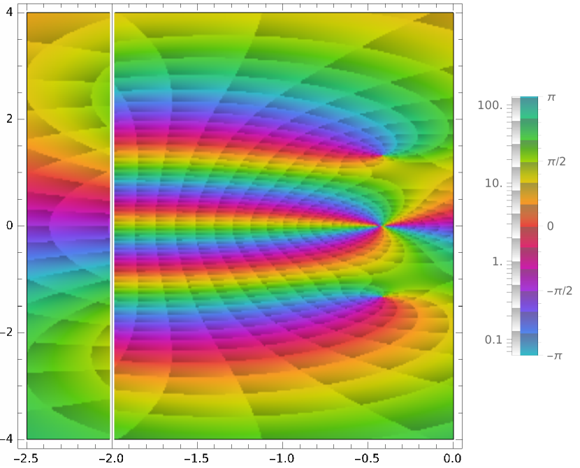
(a) $|\mathbf{k}|=1$

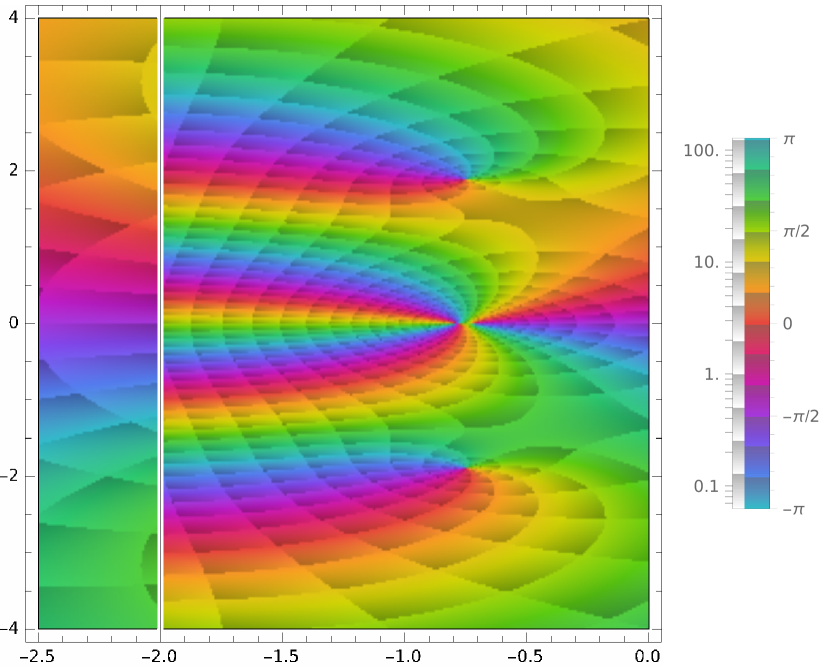
(b) $|\mathbf{k}|=\sqrt{2}$

Figure 4.1. Argument plot of the spectral function (4.44) for $\tau=0.5$ and different values of $|\mathbf{k}|$. The zeros of the function (4.44) in the complex plane define eigenvalues of the linearized BGK operator. These are points, were a small, counter-clockwise loop runs through the whole rainbow according to multiplicity.

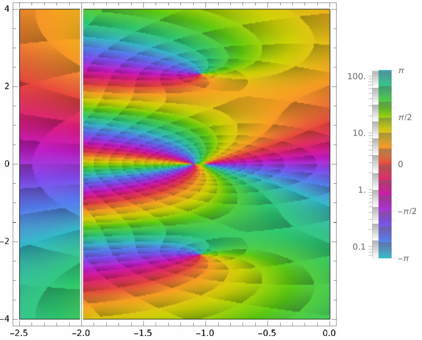
(a) $|\mathbf{k}|=\sqrt{3}$

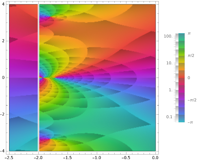
(b) $|\mathbf{k}|=\sqrt{6}$

Figure 4.2. Argument plot of the spectral function (4.44) for $\tau=0.5$ and different values of $|\mathbf{k}|$. The zeros of the function (4.44) in the complex plane define eigenvalues of the linearized BGK operator. These are points, were a small, counter-clockwise loop runs through the whole rainbow according to multiplicity. As we approach the critical wave number, the zeros move closer and closer to the essential spectrum ($\Re\lambda=-\frac{1}{\tau}$)

.

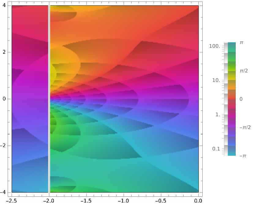
(a) $|\mathbf{k}|=\sqrt{8}$

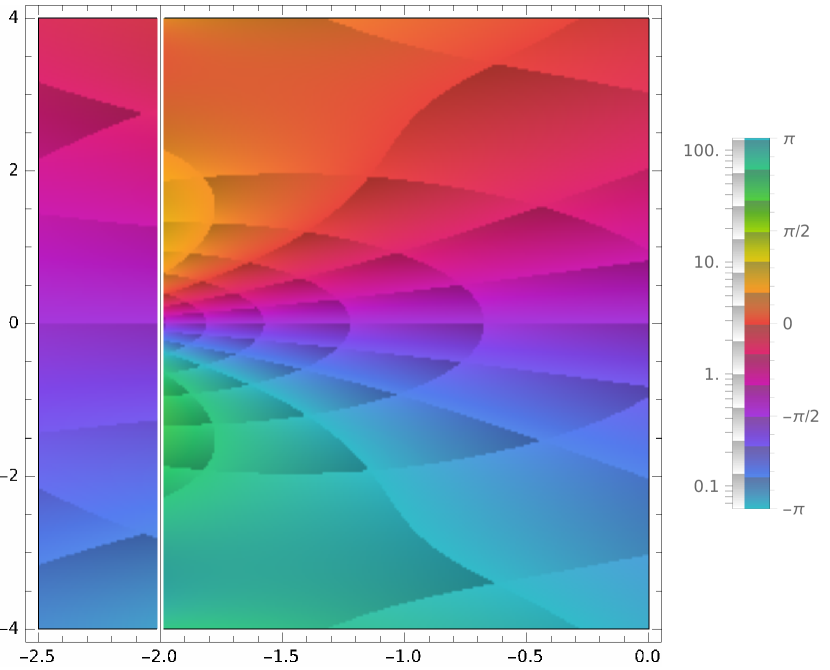
(b) $|\mathbf{k}|=3$

Figure 4.3. Argument plot of the spectral function (4.44) for $\tau=0.5$ and different values of $|\mathbf{k}|$. The zeros of the function (4.44) in the complex plane define eigenvalues of the linearized BGK operator. These are points, were a small, counter-clockwise loop runs through the whole rainbow according to multiplicity. Since the wave number is above $k_{crit}$, there exist, indeed, no zeros.

Proof.

First, let us recall that any discrete eigenvalue $\lambda$ of $\hat{\mathcal{L}}_{\mathbf{k}}$ (and hence of $\mathcal{L}$) satisfies

$$-\frac{1}{\tau}<\Re\lambda\leq 0,$$ (4.47)

by (4.9), which we will assume henceforth (of course, it would in fact follow from a slightly more detailed analysis of the following). Since $\lambda$ and $\zeta$ are related by

$$\lambda=-\frac{\mathrm{i}|\mathbf{k}|\tau\zeta+1}{\tau},$$ (4.48)

this implies that $\Re\lambda=|\mathbf{k}|\Im\zeta-\frac{1}{\tau}$ and consequently

$$0<\Im\zeta\leq\frac{1}{\tau|\mathbf{k}|}.$$ (4.49)

Our strategy is to apply Rouché’s theorem to the function $\Gamma_{\tau|\mathbf{k}|}$ by splitting it into a dominant part plus an (asymptotically) small part. To this end, we can focus on the family of rectangles $\mathbf{R}_{a}=\{-a,a,a+\mathrm{i}\frac{1}{\tau|\mathbf{k}|},-a+\mathrm{i}\frac{1}{\tau|\mathbf{k}|}\}$ for $a>0$. First, let us consider the asymptotics of $\Gamma_{\tau|\mathbf{k}|}$ in $\zeta$ for fixed $\tau|\mathbf{k}|$.
Since we are focused on the upper half-plane, we can consider $Z_{+}$ defined in (A.10) as an analytic continuation together with its limit on the real line. In particular, we see from the asymptotics (A.15) that

$$\begin{split}\Gamma_{\tau|\mathbf{k}|}(z)&\sim\frac{1}{6}\left(\zeta+6\mathrm{i}|\mathbf{k}|^{3}\tau^{3}-\zeta(\zeta^{2}+5)|\mathbf{k}|^{2}\tau^{2}+2\mathrm{i}(\zeta^{2}+3)|\mathbf{k}|\tau\right.\\ &\qquad\left.+Z(\zeta)(\zeta^{2}-(\zeta^{4}+4\zeta^{2}+11)|\mathbf{k}|^{2}\tau^{2}+2\mathrm{i}\zeta^{3}|\mathbf{k}|\tau-5)-4\mathrm{i}Z^{2}(\zeta)((\zeta^{2}+1)|\mathbf{k}|\tau-\mathrm{i}\zeta)\right)\\ &\sim\frac{1}{6}\left(\zeta+6\mathrm{i}|\mathbf{k}|^{3}\tau^{3}-\zeta(\zeta^{2}+5)|\mathbf{k}|^{2}\tau^{2}+2\mathrm{i}(\zeta^{2}+3)|\mathbf{k}|\tau\right.\\ &\qquad-\sum_{n=0}^{\infty}\frac{(2n-1)!!}{\zeta^{2n+1}}(\zeta^{2}-(\zeta^{4}+4\zeta^{2}+11)|\mathbf{k}|^{2}\tau^{2}+2\mathrm{i}\zeta^{3}|\mathbf{k}|\tau-5)\\ &\qquad\left.-4\mathrm{i}\left(-\sum_{n=0}^{\infty}\frac{(2n-1)!!}{\zeta^{2n+1}}\right)^{2}((\zeta^{2}+1)|\mathbf{k}|\tau-\mathrm{i}\zeta)\right),\end{split}$$ (4.50)

which, after rearranging and regrouping higher-order terms in $\zeta^{-1}$, gives

$$\begin{split}\Gamma_{\tau|\mathbf{k}|}(z)&\sim\frac{1}{6}\left(\zeta+6\mathrm{i}|\mathbf{k}|^{3}\tau^{3}-\zeta(\zeta^{2}+5)|\mathbf{k}|^{2}\tau^{2}+2\mathrm{i}(\zeta^{2}+3)|\mathbf{k}|\tau\right.\\ &\qquad-(\zeta^{-1}+\zeta^{-3})(\zeta^{2}-(\zeta^{4}+4\zeta^{2}+11)|\mathbf{k}|^{2}\tau^{2}+2\mathrm{i}\zeta^{3}|\mathbf{k}|\tau-5)+\mathcal{O}(|\zeta|^{-1})\\ &\qquad\left.-4\mathrm{i}\zeta^{-2}((\zeta^{2}+1)|\mathbf{k}|\tau-\mathrm{i}\zeta)\right)+\mathcal{O}(|\zeta|^{-2})\\ &\sim\frac{1}{6}\left(\zeta+6\mathrm{i}|\mathbf{k}|^{3}\tau^{3}-|\mathbf{k}|^{2}\tau^{2}\zeta^{3}-5|\mathbf{k}|^{2}\tau^{2}\zeta+2\mathrm{i}|\mathbf{k}|\tau\zeta^{2}+6\mathrm{i}|\mathbf{k}|\tau\right.\\ &\qquad-\zeta+|\mathbf{k}|^{2}\tau^{2}\zeta^{3}+4|\mathbf{k}|^{2}\tau^{2}\zeta+11|\mathbf{k}|^{2}\tau^{2}\zeta^{-1}-2\mathrm{i}|\mathbf{k}|\tau\zeta^{2}-5\zeta^{-1}\\ &\qquad-\zeta^{-1}+|\mathbf{k}|^{2}\tau^{2}\zeta+4|\mathbf{k}|^{2}\tau^{2}\zeta^{-1}+11|\mathbf{k}|^{2}\tau^{2}\zeta^{-2}-2\mathrm{i}|\mathbf{k}|\tau-5\zeta^{-3}\\ &\left.\qquad-4\mathrm{i}|\mathbf{k}|\tau-4\mathrm{i}|\mathbf{k}|\tau\zeta^{-2}-4\zeta^{-1}+\mathcal{O}(|\zeta|^{-1})\right)\\ &\sim\mathrm{i}(|\mathbf{k}|\tau)^{3}+\mathcal{O}(|\zeta|^{-1}),\end{split}$$ (4.51)

for $|\arg(\zeta)|\leq\frac{\pi}{2}-\delta,\quad\zeta\to\infty$, for any real number $0<\delta\leq\frac{\pi}{2}$.

Remark 4.3.

It is a quite remarkable property of the spectral function $\Gamma_{\tau|\mathbf{k}|}$ that all the polynomial terms (up to order four) cancel exactly with the negative-power terms in the asymptotic expansion (A.15) to give a constant asymptotic value in the limit. This is due to a subtle fine-tuning of the numerical coefficients of the polynomials. This property also guarantees the existence of a critical wave number (and hence implies that there are only finitely many discrete eigenvalues above the essential spectrum). At the outset, it is by no means clear that the spectrum should exhibit this cancellation property. Indeed, numerical investigations actually leave this question unanswered [27].

Let us start with estimating $\Gamma_{\tau|\mathbf{k}|}-\mathrm{i}(|\mathbf{k}|\tau)^{3}$ on the real line. Because $x\mapsto|\Gamma_{\tau|\mathbf{k}|}(x)-\mathrm{i}(|\mathbf{k}|\tau)^{3}|$ is an even function for $x\in\mathbb{R}$, we can focus on $x>0$. Since $\Gamma_{\tau|\mathbf{k}|}(x)\to\mathrm{i}(|\mathbf{k}|\tau)^{3}$ as $x\to\infty$, we know that $x\mapsto|\Gamma_{\tau|\mathbf{k}|}(x)-\mathrm{i}(|\mathbf{k}|\tau)^{3}|$ is bounded on the real line. Since $\Gamma_{\tau|\mathbf{k}|}(x)-\mathrm{i}(|\mathbf{k}|\tau)^{3}$ only contains powers of $|\mathbf{k}|$ up to order two, we know that there exists a $k_{1}>0$ such that

$$|\Gamma_{\tau|\mathbf{k}|}(x)-\mathrm{i}(|\mathbf{k}|\tau)^{3}|<(|\mathbf{k}|\tau)^{3},$$ (4.52)

for all $x\in\mathbb{R}$ and all $|\mathbf{k}|>k_{1}$.
By the same token, we conclude that $x\mapsto|\Gamma_{\tau|\mathbf{k}|}(x+\frac{\mathrm{i}}{|\mathbf{k}|\tau})-\mathrm{i}(|\mathbf{k}|\tau)^{3}|$, is bounded for $x\in\mathbb{R}$ since (4.50) holds in cone containing the real axis. Therefore, since again $\Gamma_{\tau|\mathbf{k}|}(x+\frac{\mathrm{i}}{|\mathbf{k}|\tau})-\mathrm{i}(|\mathbf{k}|\tau)^{3}$ is bounded for $x\in\mathbb{R}$, there exists a $k_{2}>0$ such that

$$\left|\Gamma_{\tau|\mathbf{k}|}\left(x+\frac{\mathrm{i}}{|\mathbf{k}|\tau}\right)-\mathrm{i}(|\mathbf{k}|\tau)^{3}\right|<(|\mathbf{k}|\tau)^{3},$$ (4.53)

for all $x\in\mathbb{R}$ and all $|\mathbf{k}|>k_{2}$. Clearly, an estimate of the form (4.53) for all $x\in\mathbb{R}$, $0\leq y\leq\frac{1}{\tau|\mathbf{k}|}$ and $|\mathbf{k}|>k_{3}$ holds true by compactness and the decay properties of $\Gamma_{\tau|\mathbf{k}|}$. This shows that, for $|\mathbf{k}|$ large enough, we can bound the function $\Gamma_{\tau|\mathbf{k}|}-\mathrm{i}(|\mathbf{k}|\tau)^{3}$ on the rectangle $\mathbf{R}_{a}$ for any $a>0$ by the modulus of $\mathrm{i}(|\mathbf{k}|\tau)^{3}$, which has no zeros in the strip at all (in particular, not in the strip $0\leq\Im\zeta\leq\frac{1}{\tau|\mathbf{k}|}$). For $|\mathbf{k}|$ large enough, Rouché’s theorem then implies that $\Gamma_{\tau|\mathbf{k}|}$ cannot have any zeros for $0\leq\Im\zeta\leq\frac{1}{\tau|\mathbf{k}|}$ either.
This proves the claim. ∎

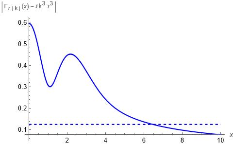
(a) On the real line

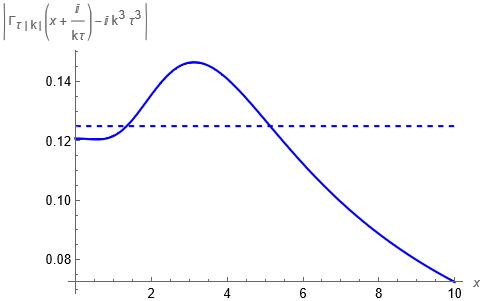
(b) For $\Im\zeta=\frac{1}{\tau|\mathbf{k}|}$

Figure 4.4. The function $\zeta\mapsto|\Gamma_{\tau|\mathbf{k}|}(\zeta)-\mathrm{i}(|\mathbf{k}|\tau)^{3}|$ on the real line and on the line $\Im\zeta=\frac{1}{\tau|\mathbf{k}|}$ for $\tau=0.5$ and $|\mathbf{k}|=1$ (solid lines) compared to $(|\mathbf{k}|\tau)^{3}$ (dashed lines).

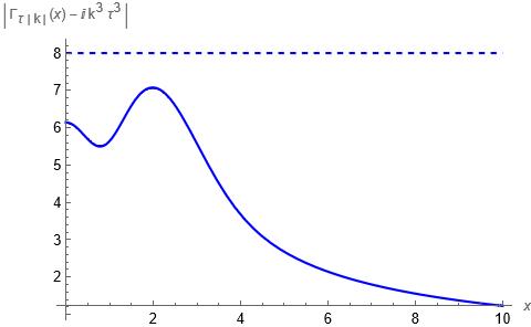
(a) On the real line

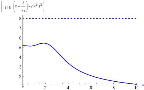
(b) For $\Im\zeta=\frac{1}{\tau|\mathbf{k}|}$

Figure 4.5. The function $\zeta\mapsto|\Gamma_{\tau|\mathbf{k}|}(\zeta)-\mathrm{i}(|\mathbf{k}|\tau)^{3}|$ on the real line and on the line $\Im\zeta=\frac{1}{\tau|\mathbf{k}|}$ for$|\mathbf{k}|=4$ (solid lines) compared to $(|\mathbf{k}|\tau)^{3}$ (dashed lines).

Now, let us prove that

$$\Gamma_{2}(\lambda):=\frac{1}{(\mathrm{i}|\mathbf{k}|\tau)^{3}}\Gamma_{\tau|\mathbf{k}|}\left(\frac{-\tau\lambda-1}{\mathrm{i}|\mathbf{k}|\tau}\right)$$ (4.54)

has exactly three zeros (one real, two complex conjugate, which we will prove later) for $|\mathbf{k}|$ small enough.

Proof.

To this end, we again use the asymptotic expansion (A.15) up to order three for the limit $|\mathbf{k}|\to 0$ together with expansion similar to those derived in (4.50) and (4.51):

$$\begin{split}\Gamma_{2}(\lambda)&\sim\frac{1}{6(\mathrm{i}|\mathbf{k}|\tau)^{3}}\left(\zeta+6\mathrm{i}|\mathbf{k}|^{3}\tau^{3}-\zeta(\zeta^{2}+5)|\mathbf{k}|^{2}\tau^{2}+2\mathrm{i}(\zeta^{2}+3)|\mathbf{k}|\tau\right.\\ &\qquad+Z(\zeta)(\zeta^{2}-(\zeta^{4}+4\zeta^{2}+11)|\mathbf{k}|^{2}\tau^{2}+2\mathrm{i}\zeta^{3}|\mathbf{k}|\tau-5)\\ &\qquad\left.-4\mathrm{i}Z^{2}(\zeta)((\zeta^{2}+1)|\mathbf{k}|\tau-\mathrm{i}\zeta)\right)\Big{|}_{\zeta=\frac{-\tau\lambda-1}{\mathrm{i}|\mathbf{k}|\tau}}\\ &\sim\frac{1}{6(\mathrm{i}|\mathbf{k}|\tau)^{3}}\left(\zeta+6\mathrm{i}|\mathbf{k}|^{3}\tau^{3}-\zeta(\zeta^{2}+5)|\mathbf{k}|^{2}\tau^{2}+2\mathrm{i}(\zeta^{2}+3)|\mathbf{k}|\tau\right.\\ &\qquad+(-\zeta^{-1}-\zeta^{-3}-3\zeta^{-5}+\mathcal{O}(|\zeta|^{-7}))(\zeta^{2}-(\zeta^{4}+4\zeta^{2}+11)|\mathbf{k}|^{2}\tau^{2}+2\mathrm{i}\zeta^{3}|\mathbf{k}|\tau-5)\\ &\qquad\left.-4\mathrm{i}(-\zeta^{-1}-\zeta^{-3}-3\zeta^{-5}+\mathcal{O}(|\zeta|^{-7}))^{2}((\zeta^{2}+1)|\mathbf{k}|\tau-\mathrm{i}\zeta)\right)\Big{|}_{\zeta=\frac{-\tau\lambda-1}{\mathrm{i}|\mathbf{k}|\tau}},\end{split}$$ (4.55)

which, after plugging in the transformation (4.48), gives

$$\begin{split}\Gamma_{2}(\lambda)&\sim\frac{1}{6(\mathrm{i}|\mathbf{k}|\tau)^{3}}\left[\mathcal{O}(|\zeta|^{-3})(|\mathbf{k}|\tau)^{2}+6\mathrm{i}(|\mathbf{k}|\tau)^{3}+(|\mathbf{k}|\tau)^{2}\left(18\zeta^{-1}+23\zeta^{-3}+33\zeta^{-5}\right)\right.\\ &\qquad\left.-2\mathrm{i}|\mathbf{k}|\tau\left(9\zeta^{-2}+18\zeta^{-4}+26\zeta^{-6}+30\zeta^{-8}+18\zeta^{-10}\right)-\left(6\zeta^{-3}+13\zeta^{-5}+24\zeta^{-7}+36\right)\right]\Big{|}_{\zeta=\frac{-\tau\lambda-1}{\mathrm{i}|\mathbf{k}|\tau}}\\ &\sim\frac{1}{6(\mathrm{i}|\mathbf{k}|\tau)^{3}}\left[6\mathrm{i}(|\mathbf{k}|\tau)^{3}+18\mathrm{i}(|\mathbf{k}|\tau)^{3}(-\tau\lambda-1)^{-1}-18\mathrm{i}(|\mathbf{k}|\tau|)(\mathrm{i}|\mathbf{k}|\tau)^{2}(-\tau\lambda-1)^{-2}\right.\\ &\qquad\left.-6(\mathrm{i}|\mathbf{k}|\tau)^{3}(-\tau\lambda-1)^{-3}+\mathcal{O}(|\mathbf{k}|^{4})\right]\\ &\sim-\frac{\lambda^{3}}{(\lambda\tau+1)^{3}}+\mathcal{O}(|\mathbf{k}|),\end{split}$$ (4.56)

i.e., in the limit $|\mathbf{k}|\to 0$, the spectral function (4.43) has a triple zero at $\lambda=0$. The cubic scaling in $|\mathbf{k}|$ in front of the above expression cancels exactly with the terms inside the bracket, leaving only the term $\lambda^{3}$ in the limit $|\mathbf{k}|\to 0$. This is consistent with the spectrum of $\hat{\mathcal{L}}_{0}$ containing zero as an isolated eigenvalue, see (4.20). By continuity of the spectrum, this implies that the there will emanate exactly three discrete eigenvalues as zeros of the spectral function $\Gamma_{\tau|\mathbf{k}|}$. ∎

4.4. Hydrodynamic Modes and their Corresponding Critical Wave Numbers

Now, let us take a closer look at the eigenvalues. From (4.43), it follows immediately that there exists a sequence of real eigenvalue of algebraic multiplicity two which we call shear mode and denote as $|\mathbf{k}|\mapsto\lambda_{shear}(|\mathbf{k}|)$.
A closer look at (4.43) reveals that the function $\Gamma_{\tau|\mathbf{k}|}$ maps imaginary numbers to imaginary numbers (since also $Z|_{\mathrm{i}\mathbb{R}}\subseteq\mathrm{i}\mathbb{R}$ by (A.6)). As a consequence, $\Gamma_{2}(\lambda)$ maps real numbers to real numbers. This shows that, together with the above considerations, that, for each wave number small enough, there exists exactly one real zero and two complex conjugated zeros. Consequently, apart from the shear mode, there exists a sequence of pairs of complex conjugated eigenvalues which we call acoustic modes and denote as $|\mathbf{k}|\mapsto\lambda_{ac}(|\mathbf{k}|)$ and $|\mathbf{k}|\mapsto\lambda_{ac}^{*}(|\mathbf{k}|)$. Figure 4.6 shows the distribution of acoustic modes for a given relaxation time and varying wave number.
Furthermore, there exists another simple, real eigenvalue called diffusion mode which we denote as $|\mathbf{k}|\mapsto\lambda_{diff}(|\mathbf{k}|)$. Each mode has its own critical wave number. In conclusion, the spectrum is given by

$$\sigma({\hat{\mathcal{L}}_{\mathbf{k}}})=\left\{-\frac{1}{\tau}+\mathrm{i}\mathbb{R}\right\}\cup\{\lambda_{shear}(|\mathbf{k}|),\lambda_{diff}(|\mathbf{k}|),\lambda_{ac}(|\mathbf{k}|),\lambda_{ac}^{*}(|\mathbf{k}|)\},$$ (4.57)

for $|\mathbf{k}|$ smaller than the respective critical wave number.

Remark 4.4.

We note that the eigenvalues (and hence the spectrum) depends on wave number only through $\tau|\mathbf{k}|$. This implies that, while the eigenvectors depend on the full wave vector $\mathbf{k}$, the form of the spectrum only depends on the dimensionless parameter $\tau|\mathbf{k}|$ and the existence of the hydrodynamic manifold (as a linear combination of eigenvectors) is independent of the relaxation time. If the relaxation time decreases, the critical wave number of each mode is increased, thus allowing for more eigenvalues in each family of modes. Consequently, decreasing the relaxation time increases the (finite) dimension of the hydrodynamic manifold.
In the limit $\tau\to 0$, the eigenvalues accumulate at the essential spectrum and we cannot separate a hydrodynamic manifold any longer, since the corresponding spectral projection does not exist (no closed contour can be defined that encircles the set of discrete eigenvalues, while not intersecting the essential spectrum).

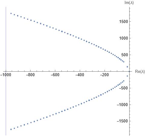
Figure 4.6. The acoustic modes for $\tau=0.001$ and wave numbers up to the critical wave number together withe the vertical line $\Re\lambda=-\frac{1}{\tau}$

To finish the spectral analysis, let us derive some information about the critical wave number of the four hydrodynamic modes. Since $|Z|\leq\sqrt{\frac{\pi}{2}}$ with equality exactly at zero (continuously extended from both sides), we immediately conclude that

$$k_{crit}(\lambda_{shear})=\sqrt{\frac{\pi}{2}}\frac{1}{\tau}\approx 1.25331\frac{1}{\tau}.$$ (4.58)

from equation (4.45). This is consistent with the result obtained in [29] (equation (2.53) in [29]).
Since the diffusion mode is real, and wanders from zero to $-\frac{1}{\tau}$ as $|\mathbf{k}|$ increases, we can recover the critical wave number by taking the limit $\lambda\to-\frac{1}{\tau}$ (on the branch $Z_{+}$) in (4.43). Since $\lim_{\zeta\to 0,\Im\zeta>0}Z(\zeta)=\mathrm{i}\sqrt{\frac{\pi}{2}}$, see (A.14), we obtain the critical wave number $k_{crit}(\lambda_{diff})$ as a zero of the cubic polynomial

$$6(k\tau)^{3}-11\sqrt{\frac{\pi}{2}}(k\tau)^{2}+\left(6+2\pi\right)k\tau-5\sqrt{\frac{\pi}{2}}=0.$$ (4.59)

The only real solution is approximately given by

$$k_{crit}(\lambda_{diff})\approx 1.35603\frac{1}{\tau}.$$ (4.60)

Now, let us turn to the acoustic mode. We know that at the critical wave number, the two complex conjugated acoustic modes will merge into the essential spectrum. This happens when $\Re\lambda=-\frac{1}{\tau}$. So, let us assume that $\lambda=-\frac{1}{\tau}-\mathrm{i}|\mathbf{k}|x$, which amount to setting $\zeta=x$ in (4.43). We obtain two equations (real and imaginary part of $\Gamma_{\tau|\mathbf{k}|}(x)$):

$$\begin{split}&\frac{1}{12}e^{-x^{2}}\left(\mathrm{erfi}\left(\frac{x}{\sqrt{2}}\right)\left(\sqrt{2\pi}(\tau|\mathbf{k}|)^{2}e^{\frac{x^{2}}{2}}\left(x^{4}+4x^{2}+11\right)-8\pi\tau|\mathbf{k}|\left(x^{2}+1\right)-\sqrt{2\pi}e^{\frac{x^{2}}{2}}\left(x^{2}-5\right)\right)\right.\\ &\qquad\left.-4\pi x\mathrm{erfi}\left(\frac{x}{\sqrt{2}}\right)^{2}-2x\left(e^{x^{2}}\left((\tau|\mathbf{k}|)^{2}\left(x^{2}+5\right)-1\right)+\sqrt{2\pi}\tau|\mathbf{k}|e^{\frac{x^{2}}{2}}x^{2}-2\pi\right)\right)=0,\\ &\frac{1}{12}e^{-x^{2}}\left(-4\pi\tau|\mathbf{k}|\left(x^{2}+1\right)\mathrm{erfi}\left(\frac{x}{\sqrt{2}}\right)^{2}+\mathrm{erfi}\left(\frac{x}{\sqrt{2}}\right)\left(8\pi x-2\sqrt{2\pi}\tau|\mathbf{k}|e^{\frac{x^{2}}{2}}x^{3}\right)+4\tau|\mathbf{k}|e^{x^{2}}\left(3\tau|\mathbf{k}|^{2}+x^{2}+3\right)\right.\\ &\qquad\left.+\sqrt{2\pi}e^{\frac{x^{2}}{2}}\left(-\left((\tau|\mathbf{k}|)^{2}\left(x^{4}+4x^{2}+11\right)\right)+x^{2}-5\right)+4\pi\tau|\mathbf{k}|\left(x^{2}+1\right)\right)=0,\end{split}$$ (4.61)

for $x\in\mathbb{R}$. The zero sets of equations (4.61) are shown in Figure 4.7.

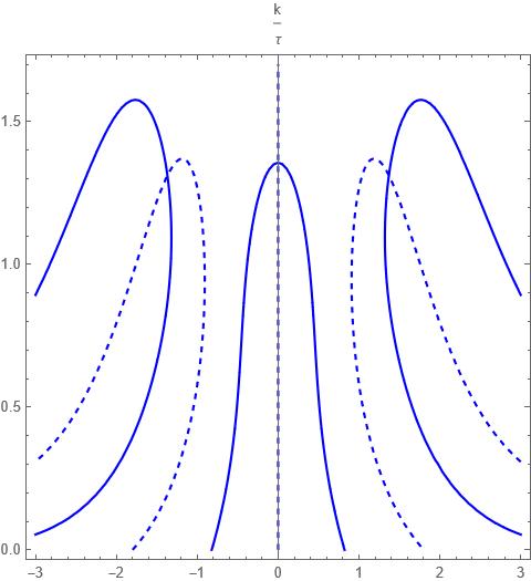
Figure 4.7. The zero sets of equations (4.61). The intersection of the solid line ($\Re\Gamma_{\tau|\mathbf{k}|}(x)$) with the dashed line ($\Im\Gamma_{\tau|\mathbf{k}|}(x)$) gives the critical wave numbers for the acoustic modes (and the diffusion mode on the real line as well).

Solving system (4.61) numerically gives the following approximation for the critical wave number of the acoustic mode:

$$k_{crit}(\lambda_{ac})=k_{crit}(\lambda_{ac}^{*})\approx 1.31176\frac{1}{\tau}.$$ (4.62)

Remark 4.5.

The critical wave numbers obtained before depend inversely on the (non-dimensional) relaxation parameter. Transforming back to physical units, we see that the critical wave number is numerically proportional to the inverse mean-free path (3.32). Indeed, we obtain that

$$k_{crit}\sim\sqrt{\frac{k_{B}T_{0}}{m}}\frac{1}{\tau_{phys}}\sim\frac{1}{l_{mfp}}.$$ (4.63)

5. Linear Hydrodynamic Manifolds

In this section, we give a description of the hydrodynamic manifolds together with their respective dynamics. We define the hydrodynamic manifold through the following properties:

1. It contains an appropriately scaled, spatially independent stationary distribution (e.g. global Maxwellian) as a base solution

2. The projection onto the hydrodynamic moments along the manifold provide a closure of the hydrodynamic moments (mass-density, velocity and temperature)

3. It attracts all trajectories in the space of probability-density functions (which are close enough to the base solution) exponentially fast, thus acting as a slow manifold

4. It is unique.

From the explicit analysis in the previous section, we know that the addition of $\mathbb{P}_{5}$ only adds finitely many discrete eigenvalues to the spectrum. Let us take a closer look at their associated eigenvectors. For each wave number $\mathbf{k}\in\mathbb{Z}^{3}$, the eigenvectors associated to $\lambda_{N}(\tau|\mathbf{k}|)$, $N\in\text{Modes}$, where $\text{Modes}=\{{\rm diff},{\rm shear},{\rm ac},{\rm ac}^{*}\}$, satisfy the equation

$$-\mathrm{i}\mathbf{v}\cdot\mathbf{k}\hat{f}_{N,j}^{eig}-\frac{1}{\tau}\hat{f}_{N,j}^{eig}+\frac{1}{\tau}\mathbb{P}_{5}\hat{f}_{N,j}^{eig}=\lambda_{N}(\tau|\mathbf{k}|)\hat{f}_{N,j}^{eig},$$ (5.1)

where $1\leq j\leq\mu_{N}(|\mathbf{k}|)$ denotes the geometric multiplicity of $\lambda_{N}(\tau|\mathbf{k}|)$. Defining

$$\alpha_{N,j,l}(\mathbf{k}):=\langle\hat{f}^{eig}_{N,j,\mathbf{k}}(\mathbf{v},\mathbf{k}),e_{l}(\mathbf{v})\rangle_{\mathbf{v}},$$ (5.2)

we can rewrite (5.1) as

$$\hat{f}^{eig}_{N,j}(\mathbf{v},\mathbf{k})=\frac{1}{\mathrm{i}\tau\mathbf{k}\cdot\mathbf{v}+1+\tau\lambda_{N}(\tau|\mathbf{k}|)}\sum_{l=0}^{4}\alpha_{N,j,l}(\mathbf{k})e_{l}(\mathbf{v}).$$ (5.3)

To omit cluttering in the notation, we will suppressed the dependence of $\alpha_{N,j,l}$ on $\mathbf{k}$. Taking an inner product with $e_{p}(\mathbf{v})$ in (5.3) gives

$$\alpha_{N,j,p}=\sum_{l=0}^{4}\alpha_{N,j,l}\int_{\mathbb{R}^{3}}e_{l}(\mathbf{v})e_{p}(\mathbf{v})\frac{e^{-\frac{|\mathbf{v}|^{2}}{2}}}{\mathrm{i}\tau\mathbf{k}\cdot\mathbf{v}+1+\tau\lambda_{N}(\tau|\mathbf{k}|)}\,d\mathbf{v},$$ (5.4)

which is equivalent to the non-invertibilty of the matrix $({\rm Id}-G_{S})$ in equation (4.29) and (4.30) for $z=-1-\tau\lambda_{N}(\tau|\mathbf{k}|)$. Indeed, denoting $\boldsymbol{\alpha}_{N,j}=(\alpha_{N,j,0},..,\alpha_{N,j,4})$, it follows that

$$\boldsymbol{\alpha}_{N,j}\in\ker(({\rm Id}-G_{S}))|_{z=-1-\tau\lambda_{N}(\tau|\mathbf{k}|)}.$$ (5.5)

This defines the eigenvector (5.3) for each wave number $\mathbf{k}$ and each mode $N$ completely.

To obtain the closure relation for the linearized hydrodynamic variables $(n_{lin},\mathbf{u}_{lin},T_{lin})$, we define a solution to the linearized dynamics (4.4) as

$$f_{hydro}(\mathbf{x},\mathbf{v},t)=\sum_{|\mathbf{k}|\leq k_{crit}}\sum_{N\in\text{Modes}}\sum_{j=1}^{\mu_{N}(\mathbf{k})}\hat{f}^{eig}_{N,j}(\mathbf{v},\mathbf{k})e^{\lambda_{N}(\tau|\mathbf{k}|)t+\mathrm{i}\mathbf{k}\cdot\mathbf{x}},$$ (5.6)

where we set

$$\hat{f}_{N,j,\mathbf{k}}^{eig}=0,\quad\text{if }|\mathbf{k}|>k_{crit}(\lambda_{N}),$$ (5.7)

and $\mu_{N}(\mathbf{k})$.
Following (3.33), let

$$\Theta:=(2\pi)^{\frac{3}{4}}\frac{v_{thermal}^{3}}{n_{0}}\begin{pmatrix}n_{0}&\mathbf{0}_{1\times 3}&0\\ \mathbf{0}_{3\times 1}&v_{thermal}I_{3\times 3}&\mathbf{0}_{3\times 1}\\ -T_{0}&\mathbf{0}_{1\times 3}&\frac{T_{0}}{3}\end{pmatrix},$$ (5.8)

denote the matrix that realized the linear coordinate change

$$(n_{lin},\mathbf{u}_{lin},T_{lin})^{T}=\Theta\mathbf{e}.$$ (5.9)

On the hydrodynamic manifold defined by (5.7), the variables $(n_{lin},\mathbf{u}_{lin},T_{lin})$ evolve according to an explicit (non-local) system. Indeed, in frequency space, denoting the Fourier coefficients of $(n_{lin},\mathbf{u}_{lin},T_{lin})$ as $(\hat{n}_{lin},\hat{\mathbf{u}}_{lin},\hat{T}_{lin})$ we find that

$$(\hat{n}_{lin},\hat{\mathbf{u}}_{lin},\hat{T}_{lin})=\Theta\mathrm{diag}(\langle\hat{f}_{hydro},\mathbf{e}\rangle)\mathbf{e},$$ (5.10)

which, setting $\boldsymbol{\alpha}_{N}=\sum_{j=1}^{\mu_{N}}\boldsymbol{\alpha}_{N,j}$ and defining

$$\boldsymbol{\alpha}:=[\boldsymbol{\alpha}_{shear},\boldsymbol{\alpha}_{diff},\boldsymbol{\alpha}_{ac},\boldsymbol{\alpha}_{ac*}],$$ (5.11)

as well as $\Lambda=\mathrm{diag}(\lambda_{shear},\lambda_{diff},\lambda_{ac},\lambda{ac*})$, $\boldsymbol{\lambda}=e^{t\Lambda}$, can be written more explicitly as

$$(\hat{n}_{lin},\hat{\mathbf{u}}_{lin},\hat{T}_{lin})=\Theta\mathrm{diag}(\boldsymbol{\alpha}\boldsymbol{\lambda})\mathbf{e}.$$ (5.12)

We can invert for $\mathbf{e}$,

$$\mathbf{e}=(\Theta\mathrm{diag}(\boldsymbol{\alpha}\boldsymbol{\lambda}))^{-1}(\hat{n}_{lin},\hat{\mathbf{u}}_{lin},\hat{T}_{lin}),$$ (5.13)

and, finally, taking a time derivative, we arrive at

$$\frac{\partial}{\partial t}(\hat{n}_{lin},\hat{\mathbf{u}}_{lin},\hat{T}_{lin})=\Theta\mathrm{diag}(\boldsymbol{\alpha}\Lambda\boldsymbol{\lambda})(\Theta\mathrm{diag}(\boldsymbol{\alpha}\boldsymbol{\lambda}))^{-1}(\hat{n}_{lin},\hat{\mathbf{u}}_{lin},\hat{T}_{lin}).$$ (5.14)

This defines a (non-local) closure to the linearized dynamics (3.1). Since - up to the conserved quantities (3.15) - any solution approaches the slow dynamics given by (5.7) exponentially fast in time, the closure (5.14) defines the unique, global, hydrodynamic limit of (3.1).

6. Conclusion and Further Perspectives

We have given a complete and (up to the solution of a transcendental equation) explicit description of the spectrum of the three-dimensional BGK equation linearized around a global Maxwellian. Further, we identified (and therefore confirmed) the existence of three families of modes (shear, diffusion and acoustic) and we gave a description of critical wave numbers. The analysis allowed us to infer that the discrete spectrum consists of a finite number of eigenvalues, thus implying that the dispersion relation remains bounded also for the acoustic modes.
Let us give an outlook on some future lines of research in this context. We expect that the results obtained in this paper are explicit enough to carry out a comparison of viscous dissipation versus capillarity as carried out in [37] for the three-dimensional Grad system.
Furthermore, the explicit knowledge of the spectral function (4.43) allows us to infer more refined approximations to the exact non-local hydrodynamics. This will involve expansions not in terms of relaxation time or wave number, but much rather in terms of the variable $\zeta$ in (4.43). This could also improve present numerical methods [27].
Finally, the spectral properties of the linear three-dimensional BGK equation will also serve as the basis for nonlinear analysis in terms of invariant manifolds. Indeed, the fact that the discrete spectrum is well separated from the essential spectrum allows us to define a spectral projection for the whole set of eigenvalues, thus giving the first-order approximation (in terms of nonlinear deformations) to the hydrodynamic manifolds. In particular, we expect that the theory of thermodynamic projectors [20] may be helpful in proving the nonlinear extension.

Data Availability Statement

All data generated or analysed during this study are included in this published article (and its supplementary information files).

Appendix A Some Properties of the Plasma Dispersion Function

In the following, we collect some properties of the integral expression (4.39). In particular, to evaluate the integral in (4.39) in terms of error functions, we rely on the identities in [1, p.297]. Let

$$w(z)=e^{-z^{2}}(1-\mathrm{erf}(-\mathrm{i}z)),\quad z\in\mathbb{C},$$ (A.1)

which satisfies the functional identity

$$w(-z)=2e^{-z^{2}}-w(z),\quad z\in\mathbb{C}.$$ (A.2)

Function (A.1) is called Faddeeva function and is frequently encountered in problems related to kinetic equations [17]. We then have that

$$w(z)=\frac{\mathrm{i}}{\pi}\int_{\mathbb{R}}\frac{e^{-s^{2}}}{z-s}\,ds,\quad\Im{z}>0,$$ (A.3)

and, by relation (A.2), we have for $\Im{z}<0$:

$$\begin{split}\frac{\mathrm{i}}{\pi}\int_{\mathbb{R}}\frac{e^{-s^{2}}}{z-s}\,ds&=-\frac{\mathrm{i}}{\pi}\int_{\mathbb{R}}\frac{e^{-s^{2}}}{(-z)+s}\,ds\\ &=-\frac{\mathrm{i}}{\pi}\int_{\mathbb{R}}\frac{e^{-s^{2}}}{(-z)-s}\,ds\\ &=-w(-z)\\ &=e^{-z^{2}}[-1-\mathrm{erf}(-\mathrm{i}z)].\end{split}$$ (A.4)

Consequently, we obtain

$$\begin{split}\int_{\mathbb{R}}\frac{1}{s-z}e^{-\frac{s^{2}}{2}}\,ds&=\int_{\mathbb{R}}\frac{e^{-s^{2}}}{s-\frac{z}{\sqrt{2}}}\,ds\\ &=\mathrm{i}\pi\frac{\mathrm{i}}{\pi}\int_{\mathbb{R}}\frac{e^{-s^{2}}}{\frac{z}{\sqrt{2}}-s}\,ds\\ &=\begin{cases}\mathrm{i}\pi e^{-\frac{z^{2}}{2}}\left[1-\mathrm{erf}\left(\frac{-\mathrm{i}z}{\sqrt{2}}\right)\right],&\quad\text{ if }\Im{z}>0,\\ \mathrm{i}\pi e^{-\frac{z^{2}}{2}}\left[-1-\mathrm{erf}\left(\frac{-\mathrm{i}z}{\sqrt{2}}\right)\right],&\quad\text{ if }\Im{z}<0,\end{cases}\end{split}$$ (A.5)

where in the first step, we have re-scaled $s\mapsto\sqrt{2}s$ in the integral. Written more compactly, we arrive at

$$Z(z)=\mathrm{i}\sqrt{\frac{\pi}{2}}e^{-\frac{z^{2}}{2}}\left[\mathrm{sign}(\Im{z})-\mathrm{erf}\left(\frac{-\mathrm{i}z}{\sqrt{2}}\right)\right],\quad\Im{z}\neq 0.$$ (A.6)

An an argument plot together with an modulus-argument plot of $Z$ are shown in Figure A.1.

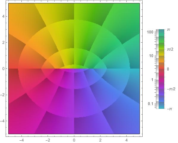
(a) Argument Plot of $Z$

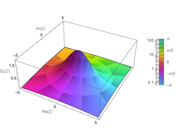
(b) Modulus-Argument Plot of $Z$

Figure A.1. Complex plots of the function Z.

Clearly, $Z$ is discontinuous across the real line (albeit that $Z|_{\mathbb{R}}$ exists in the sense of principal values as the Hilbert transform of a real Gaussian [13]). The properties

$$\begin{split}|Z(z)|\leq\sqrt{\frac{\pi}{2}},&\text{ for }z\in\mathbb{C}\setminus\mathbb{R},\\ 0<\arg Z(z)<\pi&\text{ for }\Im(z)>0,\\ -\pi<\arg Z(z)<0&\text{ for }\Im(z)<0,\end{split}$$ (A.7)

are easy to show and can be read off from the plots (A.1) directly as well.
Function (A.6) satisfies an ordinary differential equation (in the sense of complex analytic functions) on the upper and on the lower half-plane. Indeed, integrating (4.39) by parts gives

$$\begin{split}1&=\frac{1}{\sqrt{2\pi}}\int_{\mathbb{R}}(v-z)\frac{e^{-\frac{v^{2}}{2}}}{v-z}\,dv=-zZ+\frac{1}{\sqrt{2\pi}}\int_{\mathbb{R}}v\frac{e^{-\frac{v^{2}}{2}}}{v-z}\,dv\\ &=-zZ-\frac{1}{\sqrt{2\pi}}\int_{\mathbb{R}}\frac{e^{-\frac{v^{2}}{2}}}{(v-z)^{2}}\,dv=-zZ-\frac{d}{dz}Z,\end{split}$$ (A.8)

which implies that $Z$ satisfies the differential equation

$$\frac{d}{dz}Z=-zZ-1,$$ (A.9)

for $z\in\mathbb{C}\setminus\mathbb{R}$. Formula (A.9) can also be used as a recurrence relation for the higher derivatives of $Z$.
Since we will be interested in function (A.6) for $\Im z$ positive and negative as global functions, we define

$$\begin{split}Z_{+}(z)&=\mathrm{i}\sqrt{\frac{\pi}{2}}e^{-\frac{z^{2}}{2}}\left[1-\mathrm{erf}\left(\frac{-\mathrm{i}z}{\sqrt{2}}\right)\right],\\ Z_{-}(z)&=\mathrm{i}\sqrt{\frac{\pi}{2}}e^{-\frac{z^{2}}{2}}\left[-1-\mathrm{erf}\left(\frac{-\mathrm{i}z}{\sqrt{2}}\right)\right],\end{split}$$ (A.10)

for all $z\in\mathbb{C}$. Both functions can be extended to analytic functions on the whole complex plane via analytic continuation.
Recall that the error function has the properties that

$$\mathrm{erf}(-z)=-\mathrm{erf}(z),\qquad\mathrm{erf}(z^{*})=\mathrm{erf}(z)^{*},$$ (A.11)

for all $z\in\mathbb{C}$, which implies that for $x\in\mathbb{R}$,

$$\mathrm{erf}(\mathrm{i}x)=-\mathrm{erf}(-\mathrm{i}x)=-\mathrm{erf}(\mathrm{i}x)^{*},$$ (A.12)

i.e, the error function maps imaginary numbers to imaginary numbers. Defining the imaginary error function,

$$\mathrm{erfi}(z):=-\mathrm{i}\mathrm{erf}(\mathrm{i}z),$$ (A.13)

for $z\in\mathbb{C}$, which, by (A.12) satisfies $\mathrm{erfi}|_{\mathbb{R}}\subset\mathbb{R}$, it follows that for $x\in\mathbb{R}$:

$$\Re Z_{+}(x)=-\sqrt{\frac{\pi}{2}}e^{-\frac{x^{2}}{2}}\mathrm{erfi}\left(\frac{x}{\sqrt{2}}\right),\quad\Im Z_{+}(x)=-\sqrt{\frac{\pi}{2}}e^{-\frac{x^{2}}{2}},$$ (A.14)

similarly for $Z_{-}(x)$.
Next, let us prove the following asymptotic expansion of $Z_{+}$:

$$Z_{+}(z)\sim-\sum_{n=0}^{\infty}\frac{(2n-1)!!}{z^{2n+1}},\qquad\text{ for }|\arg(z)|\leq\frac{\pi}{2}-\delta,\qquad z\to\infty,$$ (A.15)

for any $0<\delta\leq\frac{\pi}{2}$. The proof will be based on a generalized version of Watson’s Lemma [41]. To this end, let us define the Laplace transform

$$\mathcal{L}[f](z)=\int_{0}^{\infty}f(x)e^{-zx}\,dx,\quad z\in\mathbb{C},$$ (A.16)

of an integrable function $f:[0,\infty)\to\mathbb{C}$.

Lemma A.1.

[Generalized Watson’s Lemma] Assume that (A.16) exists for some $z=z_{0}\in\mathbb{C}$ and assume that $f$ admits an asymptotic expansion of the form

$$f(x)=\sum_{n=0}^{N}a_{n}x^{\beta_{n}-1}+o(x^{\beta_{N}-1}),\qquad x>0,\quad x\to 0,$$ (A.17)

where $a_{n}\in\mathbb{C}$ and $\beta_{n}\in\mathbb{C}$ with $\Re\beta_{0}>0$ and $\Re\beta_{n}>\Re\beta_{n-1}$ for $1\leq n\leq N$. Then $\mathcal{L}[f](z)$ admits an asymptotic expansion of the form

$$\mathcal{L}[f](z)=\sum_{n=0}^{N}a_{n}\Gamma(\beta_{n})z^{-\beta_{n}}+o(z^{-\beta_{N}}),\quad v,\quad z\to\infty,$$ (A.18)

for any real number $0<\delta\leq\frac{\pi}{2}$, where $\Gamma$ is the standard Gamma function.

For a proof of the above Lemma, we refer e.g. to [16]. Classically, Lemma (A.1) is applied to prove that the imaginary error function admits an asymptotic expansion for $x\in\mathbb{R}$ of the form

$$\mathrm{erfi}(x)\sim\frac{e^{x^{2}}}{\sqrt{\pi}x}\sum_{k=0}^{\infty}\frac{(2k-1)!!}{(2x^{2})^{k}},\qquad\text{ for }x>0,\quad x\to\infty,$$ (A.19)

see also [31], based on the classical version of Watson’s Lemma, whose assumptions are, however, unnecessarily restrictive [43].

For completeness, we recall the derivation of (A.15) based on Lemma A.1. First, let us rewrite $\mathrm{erfi}$ as a Laplace transform using the change of variables $t=\sqrt{1-s}$ with $dt=\frac{ds}{2\sqrt{1-s}}$

$$\begin{split}\mathrm{erfi}(z)&=\int_{0}^{1}\frac{d}{dt}\mathrm{erfi}(tz)\,dt=\frac{2z}{\sqrt{\pi}}\int_{0}^{1}e^{t^{2}z^{2}}\,dt=\frac{2z}{\sqrt{\pi}}\int_{0}^{1}e^{z^{2}(1-s)}\,\frac{ds}{2\sqrt{1-s}}\\ &=\frac{ze^{z^{2}}}{\sqrt{\pi}}\int_{0}^{1}\frac{1}{\sqrt{1-s}}e^{-sz^{2}}\,ds=\frac{ze^{z^{2}}}{\sqrt{\pi}}\int_{0}^{\infty}\frac{\chi_{[0,1]}(s)}{\sqrt{1-s}}e^{-sz^{2}}\,ds.\end{split}$$ (A.20)

From the Taylor expansion of the Binomial function, we know that

$$\frac{1}{\sqrt{1-s}}=\sum_{n=0}^{\infty}{-\frac{1}{2}\choose n}(-s)^{n}=\sum_{n=0}^{\infty}4^{-n}{2n\choose n}s^{n},$$ (A.21)

which allows us to apply Lemma (A.1) with $\beta_{n}=n+1$ and $a_{n}=4^{-n}{2n\choose n}$, thus leading to

$$\begin{split}\mathrm{erfi}(z)&\sim\frac{ze^{z^{2}}}{\sqrt{\pi}}\sum_{n=0}^{\infty}4^{-n}{2n\choose n}\Gamma(n+1)z^{-2(n+1)}\\ &\sim\frac{e^{z^{2}}}{\sqrt{\pi}}\sum_{n=0}^{\infty}\frac{(2n)!}{4^{n}n!}z^{-2n-1}\\ &\sim\frac{e^{z^{2}}}{z\sqrt{\pi}}\sum_{n=0}^{\infty}\frac{(2n-1)!!}{(2z)^{n}},\end{split}$$ (A.22)

for $z\to\infty$ and $|\arg(z)|\leq\frac{\pi}{2}-\delta$, $0<\delta\leq\frac{\pi}{2}$. This is consistent with formula (A.19) for the limit along the real line. Finally, we arrive at the following asymptotic expansion for $Z$:

$$Z_{+}(z)\sim\mathrm{i}\sqrt{\frac{\pi}{2}}e^{-\frac{z^{2}}{2}}-\sum_{n=0}^{\infty}\frac{(2n-1)!!}{z^{2n+1}},\qquad\text{ for }|\arg(z)|\leq\frac{\pi}{2}-\delta,\qquad z\to\infty,$$ (A.23)

which is, of course, equivalent to

$$Z_{+}(z)\sim-\sum_{n=0}^{\infty}\frac{(2n-1)!!}{z^{2n+1}},\qquad\text{ for }|\arg(z)|\leq\frac{\pi}{2}-\delta,\qquad z\to\infty,$$ (A.24)

since $|e^{-z^{2}}|^{2}=e^{-2(x^{2}-y^{2})}\to 0$ for $\Re{z}=x\to\infty$.

References

- [1] M. Abramowitz and I. A. Stegun. Handbook of mathematical functions with formulas, graphs, and mathematical tables, volume 55. US Government printing office, 1948.
- [2] C. Bardos, F. Golse, and C. D. Levermore. Fluid dynamic limits of kinetic equations ii. Convergence proofs for the Boltzmann equation. Communications on pure and applied mathematics, 46(5):667–753, 1993.
- [3] P. L. Bhatnagar, E. P. Gross, and M. Krook. A model for collision processes in gases. I. small amplitude processes in charged and neutral one-component systems. Physical review, 94(3):511, 1954.
- [4] A. Bobylev. The Chapman-Enskog and Grad methods for solving the Boltzmann equation. In Akademiia Nauk SSSR Doklady, volume 262, pages 71–75, 1982.
- [5] A. Bobylev. The theory of the nonlinear spatially uniform Boltzmann equation for Maxwell molecules. Soviet Scientific Reviews. Section C, 7, 01 1988.
- [6] A. V. Bobylev. Instabilities in the Chapman–Enskog expansion and hyperbolic Burnett equations. Journal of statistical physics, 124(2):371–399, 2006.
- [7] R. E. Caflisch. The Boltzmann equation with a soft potential. Communications in Mathematical Physics, 74(1):71–95, 1980.
- [8] T. Carleman. Problemes mathématiques dans la théorie cinétique des gaz, volume 2. Almqvist & Wiksells boktr., 1957.
- [9] T. Carty. Grossly determined solutions for a Boltzmann-like equation. Kinetic and Related Models, 10(4):957–976, 2017.
- [10] T. E. Carty. Elementary solutions for a model Boltzmann equation in one dimension and the connection to grossly determined solutions. Physica D: Nonlinear Phenomena, 347:1–11, 2017.
- [11] C. W. Chang, J. Foch, G. W. Ford, and G. E. Uhlenbeck. Studies in Statistical Mechanics. North-Holland, 1970.
- [12] S. Chapman and T. Cowling. The Mathematical Theory of Non-uniform Gases: An Account of the Kinetic Theory of Viscosity, Thermal Conduction and Diffusion in Gases. Cambridge Mathematical Library. Cambridge University Press, 1990.
- [13] B. Conte and S. Conte. The Plasma Dispersion Function: The Hilbert Transform of the Gaussian. Academic Press, 1961.
- [14] L. Desvillettes, C. Mouhot, and C. Villani. Celebrating Cercignani’s conjecture for the Boltzmann equation. Kinetic and Related Models, 4, 09 2010.
- [15] R. S. Ellis and M. A. Pinsky. The first and second fluid approximations to the linearized Boltzmann equation. J. Math. Pures Appl, 54(9):125–156, 1975.
- [16] A. Erdélyi. General asymptotic expansions of Laplace integrals. Archive for Rational Mechanics and Analysis, 7(1):1–20, 1961.
- [17] R. Fitzpatrick. Plasma Physics: An Introduction. Taylor & Francis, 2014.
- [18] A. Gorban and I. Karlin. Hilbert’s 6th problem: Exact and approximate hydrodynamic manifolds for kinetic equations. Bulletin of the American Mathematical Society, 51:186–246, 11 2013.
- [19] A. N. Gorban and I. V. Karlin. Method of invariant manifolds and regularization of acoustic spectra. Transport Theory and Statistical Physics, 23:559–632, 1994.
- [20] A. N. Gorban and I. V. Karlin. Uniqueness of thermodynamic projector and kinetic basis of molecular individualism. Physica A: Statistical Mechanics and its Applications, 336(3):391–432, 2004.
- [21] A. N. Gorban and I. V. Karlin. Invariant Manifolds for Physical and Chemical Kinetics, volume 660 of Lecture Notes in Physics. Springer Science & Business Media, 2005.
- [22] H. Grad. On the kinetic theory of rarefied gases. Communications on pure and applied mathematics, 2(4):331–407, 1949.
- [23] H. Grad. Asymptotic theory of the Boltzmann equation. The physics of Fluids, 6(2):147–181, 1963.
- [24] H. Grad. Asymptotic equivalence of the Navier–Stokes and nonlinear Boltzmann equations. Magneto-Fluid Dynamics Division, Courant Institute of Mathematical Sciences, 1964.
- [25] D. Hilbert. Grundzüge einer allgemeinen Theorie der linearen Integralgleichungen, volume 3. BG Teubner, 1912.
- [26] D. Hilbert et al. Mathematical problems. Bulletin of American Mathematical Society, 37(4):407–436, 2000.
- [27] I. V. Karlin, M. Colangeli, and M. Kröger. Exact linear hydrodynamics from the Boltzmann equation. Physical Review Letters, 100(21):214503, 2008.
- [28] F. Kogelbauer. Slow hydrodynamic manifolds for the three-component linearized Grad system. Continuum Mechanics and Thermodynamics, Aug 2019.
- [29] F. Kogelbauer. Non-local hydrodynamics as a slow manifold for the one-dimensional kinetic equation. Continuum Mechanics and Thermodynamics, 33, 03 2021.
- [30] P. Kurasov and S.-T. Kuroda. Krein’s resolvent formula and perturbation theory. Journal of Operator Theory, pages 321–334, 2004.
- [31] F. Olver. Asymptotics and special functions. AK Peters/CRC Press, 1997.
- [32] B. Perthame. Global existence to the BGK model of Boltzmann equation. Journal of Differential equations, 82(1):191–205, 1989.
- [33] B. Perthame and M. Pulvirenti. Weighted bounds and uniqueness for the Boltzmann BGK model. Archive for rational mechanics and analysis, 125(3):289–295, 1993.
- [34] P. Rosenau. Extending hydrodynamics via the regularization of the Chapman–Enskog expansion. Phys. Rev. A, 40:7193–7196, Dec 1989.
- [35] L. Saint-Raymond. Discrete time Navier–Stokes limit for the BGK Boltzmann equation. Comm. in Partial Differential Equations, 27(1 and 2):149–184, 08 2006.
- [36] L. Saint-Raymond. A mathematical PDE perspective on the Chapman–Enskog expansion. Bulletin of the American Mathematical Society, 51(2):247–275, 2014.
- [37] M. Slemrod. Chapman–Enskog viscosity-capillarity. Quarterly of Applied Mathematics, 70(3):613–624, 2012.
- [38] G. Teschl. Jacobi operators and completely integrable nonlinear lattices. Number 72. American Mathematical Soc., 2000.
- [39] C. Truesdell and R. G. Muncaster. Fundamentals of Maxwel’s Kinetic Theory of a Simple Monatomic Gas: Treated as a Branch of Rational Mechanics. Academic Press, 1980.
- [40] C. Villani. Hypocoercivity. arXiv preprint math/0609050, 2006.
- [41] G. N. Watson. The harmonic functions associated with the parabolic cylinder. Proceedings of the London Mathematical Society, s2-17(1):116–148, 1918.
- [42] A. Weinstein. On nonselfadjoint perturbations of finite rank. Journal of Mathematical Analysis and Applications, 45(3):604–614, 1974.
- [43] R. Wong and M. Wyman. Generalization of Watson’s lemma. Canadian Journal of Mathematics, 24(2):185–208, 1972.