Quantum interference in the resonance fluorescence of a $J=1/2-J^{\prime}=1/2$
atomic system: Quantum beats, nonclassicality, and non-Gaussianity

Abstract

We study theoretically quantum statistical and spectral properties of the resonance fluorescence of a single atom or system with angular momentum $J=1/2-J^{\prime}=1/2$ driven by a monochromatic linearly polarized laser field, due to quantum interference among its two antiparallel, $\pi$ transitions. A magnetic field parallel to the laser polarization is applied to break the degeneracy (Zeeman effect). In the nondegenerate case, the $\pi$ transitions evolve at different generalized Rabi frequencies, producing quantum beats in the intensity and the dipole-dipole, intensity-intensity, and quadrature-intensity correlations. For a strong laser and large Zeeman splitting the beats have mean and modulation frequencies given by the average and difference, respectively, of the Rabi frequencies, unlike the beats studied in many spectroscopic systems, characterized by a modulated exponential-like decay. Further, the Rabi frequencies are those of the pairs of sidebands of the Mollow-like spectrum of the system. In the two-time correlations, the cross contributions, i.e., those with products of probability amplitudes of the two $\pi$ transitions, have a lesser role than those from the interference of the probability densities. In contrast, there are no cross terms in the total intensity.We also consider nonclassical and non-Gaussian properties of the phase-dependent fluorescence for the cases of weak to moderate excitation and in the regime of beats. The fluorescence in the beats regime is nonclassical, mainly from third-order dipole fluctuations, which reveal them to be also strongly non-Gaussian, and their quadrature spectra show complex features around the Rabi frequencies. For small laser and Zeeman detunings, a weak to moderate laser field pumps the system partially to one of the ground states, showing slow decay in the two-time correlations and a narrow peak in the quadrature spectra.

I Introduction

In spectroscopy, quantum beats are the modulation of the spontaneous emission decay of a multilevel system due to the energy difference among its excited or its ground states, the beats resulting from the indeterminacy of a photon’s path when observed by a broadband detector. Two-level systems with degenerate upper and ground levels can have their levels split with a magnetic field and give way to quantum beats. In recent weak field cavity QED experiments beats were observed from spontaneous emissions to the ground states [1, 2]. As is often the case of beats using ground states, a higher-order process may be required to establish the coherence among them and then observe beats in intensity correlations [3]. The variety of schemes and conditions to produce quantum beats is too big to consider here, see Ref.[4, 5, 6].

Resonance fluorescence, the continued spontaneous emission by atoms under laser excitation, is a well-established means in quantum optics for the study of, among others: nonclassical properties of the field [7], such as antibunching and squeezing; atomic coherence [6], such as electromagnetically induced transparency; and in atomic physics with laser cooling and trapping [8] and atomic structure [9], such as determination of transition frequencies and level shifts.

Recently, the properties of the resonance fluorescence of a single atomic system with angular momentum transition $J=1/2-J^{\prime}=1/2$ driven by a monochromatic laser have been the subject of great interest due to the possibility of observing vacuum-induced coherence effects due to interference among the two antiparallel $\pi$ transitions, emitting into the same frequency range of the electromagnetic vacuum. Here, the $\pi$ transitions are incoherently coupled, mediated by spontaneous emission in the $\sigma$ transitions, and excited again by the laser. Being the dipoles of the transitions antiparallel it is now realistic to observe interference effects, while the $V$ and $\Lambda$ three-level systems require additional preparation because the transitions are perpendicular [6, 10]. Particular attention has been devoted to the spectrum [11, 12, 13, 14], time-energy complementarity [12, 13], Young’s interference [15], phase shifts [16], nonclassical properties of the fluorescence via squeezing [17], photon correlations [18], frequency-resolved photon correlations [19], and cooperative effects in photon correlations [20]. Also, the case of additional laser excitation of one of the $\sigma$ transitions on the spectrum and squeezing has been studied in [21, 22, 23]. Curiously, in those works, there is no mention of quantum beats, which are among the more familiar manifestations of quantum interference.

In this paper, we investigate theoretically quantum interference effects, nonclassicality, and non-Gaussianity of the resonance fluorescence light from the $\pi$ transitions of a single $J=1/2-J^{\prime}=1/2$ atomic system driven by a linearly polarized laser and a magnetic field to break the degeneracy. Both the unequal Zeeman splittings for ground and excited levels and the laser-induced ac Stark effect makes the effective transition frequencies different and also the $\pi$ transitions evolve with different generalized Rabi frequencies $\Omega_{1}$ and $\Omega_{2}$; these determine dynamical and spectral properties. Resonance fluorescence in this system then goes beyond pure spontaneous emission, and the generalized Rabi frequencies replace energy-level splittings. For a start, we illustrate the evolution of the state populations, an aspect bypassed previously in favor of their steady-state values, which helps us to understand the origin of interference in this system.

As a major result, we find the emergence of quantum beats due to the interference of light from the $\pi$ transitions in the nondegenerate situation. For weak laser and magnetic fields $\Omega_{1}$ and $\Omega_{2}$ are nearly equal, so the beats have simple damped oscillatory behavior or just damped decay. For strong laser and magnetic fields, on the other hand, the generalized Rabi frequencies split enough such that the beats evolve to damped wave packets with well-defined oscillations at the average frequency $(\Omega_{1}+\Omega_{2})/2$ and modulation frequency $(\Omega_{2}-\Omega_{1})/2$. There are no beats in the degenerate case.

We study quantum beats in the fluorescence intensity, where an initial condition with unequal ground state populations is needed, and in two-time correlations such as dipole-dipole (to calculate spectra), intensity-intensity [24, 25], and phase-dependent intensity-amplitude correlations [26, 27]. For the two-time correlations it is only necessary that the dominant terms in the correlation be initially nonzero. An early hint for the appearance of beats may be seen in the closeness of sidebands in the spectrum at the frequencies $\pm\Omega_{1}$ and $\pm\Omega_{2}$ [13]; the corresponding dipole correlation in the Wiener-Khinchine formula exhibits strongly damped quantum beats.

While beats may be obtained from incoherent sources [28] some form of coherence is needed. One may ask if the vacuum-induced coherence (VIC), the coupling of the upper states (in this case) by the reservoir, is such. In this paper, the incoherent sources are the $\pi$ transitions emitting photons spontaneously. These transitions are incoherently coupled by the spontaneous emission in the $\sigma$ transitions. Coherence is maintained because all emissions make the atom end up in one ground state or the other, i.e., the system is closed, see Fig. 1. We find that the cross terms in the correlations that link both $\pi$ transitions, the signature of VIC, are small compared to those of interference from the single transitions. This is also observed in the contributions to the total intensity from the coherent and incoherent parts.

Figure 1: Scheme of the $J=1/2$ – $J=1/2$ atomic system interacting with a laser driving the $|1\rangle-|3\rangle$ and $|2\rangle-|4\rangle$ transitions with Rabi frequency $\Omega$ and detuning $\Delta$. There are spontaneous decay rates $\gamma_{1}$, $\gamma_{2}$ and $\gamma_{\sigma}$, vacuum-induced coherence $\gamma_{12}$, and Zeeman frequency splittings $B_{\ell}$ and $B_{u}$.

The two-time amplitude-intensity correlation (AIC) is a measurement that probes up to third-order quadrature fluctuations that may violate classical inequalities [26, 27]; single few-level atom resonance fluorescence does [29, 30, 31, 32, 33]. In the weak-field regime, the AIC is reduced to a second-order detection, i. e., of squeezed light [7], and the fluctuations are Gaussian. For stronger laser fields, squeezing, if any, is mixed with third-order fluctuations. In this nonlinear interaction case, with quantum beats as a notable feature, the light’s fluctuations are also non-Gaussian. The AIC becomes a tool for studying non-Gaussianity of light, in both the time and frequency domains.

We work around two regimes in the parameter space: (i) the Rabi frequency, laser detuning and the difference Zeeman splittings are close to the spontaneous emission rate, enough to exhibit beats, but there is some squeezing, and (ii) where both laser and magnetic fields are strong, with well-developed beats that contribute to large third-order nonclassical and non-Gaussian fluctuations.

Finally, we also analyze squeezing via the variance or total noise [34], finding that the total squeezing is limited to a region in parameter space of small laser and Zeeman detunings, and the laser intensity should be even smaller than in the two-level atom case. Beats are usually well outside the squeezing region.

The paper is organized as follows. After describing the model’s main features in Sec. II, we discuss the basic dynamic and stationary properties of the atomic expectation values in Sec. III. Then, in Sec. IV, we describe the scattered field intensity and its fluctuations. Secs. V-VII are devoted to two-time correlation functions. In Sec. V, we relate the double sideband spectrum [13] with beats in the dipole-dipole correlation function. Then, in Sec. VI, we study Brown-Twiss photon-photon correlations [24, 25], extending the work of Ref.[18] to the nondegenerate case. Section VII is devoted to phase-dependent fluctuations by conditional homodyne detection [26, 27] in both the temporal and spectral domains. In Sec. VIII, we consider squeezing of fluctuations using the variance. We close in Sec. IX with a discussion and conclusions. Two Appendices detail solution methods, initial conditions, and optimal appearance of beats.

II Model

The system, illustrated in Fig. 1, consists of a two-level atom with transition $J=1/2$ – $J=1/2$ and states with magnetic quantum number $m=\pm J$,

$$|1\rangle = |J,-1/2\rangle,\qquad|2\rangle=|J,1/2\rangle,$$

$$|3\rangle = |J,-1/2\rangle,\qquad|4\rangle=|J,1/2\rangle.$$ (1)

The matrix elements are

$$\mathbf{d}_{1} = \langle 1|\hat{\mathbf{d}}|3\rangle=-\frac{1}{\sqrt{3}}\mathcal{D}\mathbf{e}_{z},\qquad\mathbf{d}_{2}=\langle 2|\hat{\mathbf{d}}|4\rangle=-\mathbf{d}_{1},$$

$$\mathbf{d}_{3} = \langle 2|\hat{\mathbf{d}}|3\rangle=\sqrt{\frac{2}{3}}\mathcal{D}\mathbf{e}_{-},\qquad\mathbf{d}_{4}=\langle 1|\hat{\mathbf{d}}|4\rangle=\mathbf{d}_{3}^{\ast},$$ (2)

where $\mathcal{D}$ is the reduced dipole matrix element. We choose the field polarization basis $\{\mathbf{e}_{z},\mathbf{e}_{-},\mathbf{e}_{+}\}$ (linear, left circular, right circular), where $\mathbf{e}_{\pm}=\mp(\mathbf{e}_{x}\pm i\mathbf{e}_{y})/2$.

The $\pi$ transitions, $|1\rangle-|3\rangle$ and $|2\rangle-|4\rangle$ ($m=m^{\prime}$), are coupled to linearly polarized light and have their dipole moments antiparallel. On the other hand, the $\sigma$ transitions, $|1\rangle-|4\rangle$ and $|2\rangle-|3\rangle$ ($m\neq m^{\prime}$), are coupled to circularly polarized light. This configuration can be found, for example, in ${}^{198}\mathrm{Hg}^{+}$ [11], and ${}^{40}\mathrm{Ca}^{+}$ [20].

The level degeneracy is removed by the Zeeman effect, applying a magnetic field $B_{z}$ along the $z$ direction. Note that the energy splittings $g\mu_{B}B_{z}$ of the upper ($u$) and lower ($\ell$) levels are different due to unequal Landé $g$ factors, $g_{u}$ and $g_{\ell}$, respectively; $\mu_{B}$ is Bohr’s magneton. The difference Zeeman splitting is

$$\delta=\frac{(g_{u}-g_{\ell})\mu_{B}B_{z}}{\hbar}=\frac{g_{u}-g_{\ell}}{g_{\ell}}B_{\ell},$$ (3)

where $B_{\ell}=g_{l}\mu_{B}B_{z}/\hbar$. For ${}^{198}\mathrm{Hg}^{+}$ $g_{u}=2/3$ and $g_{\ell}=2$, so $\hbar\delta=-(4/3)\mu_{B}B_{z}=-(2/3)\hbar B_{\ell}$.

The atom is driven by a monochromatic laser of frequency $\omega_{L}$, linearly polarized in the $z$ direction, propagating in the $x$ direction,

$$\mathbf{E}_{L}(x,t) = E_{0}e^{i(\omega_{L}t-k_{L}x)}\mathbf{e}_{z}+\mathrm{c.c.},$$ (4)

thus driving only the $\pi$ transitions.

The free atomic, $H_{0}$, and interaction, $V$, parts of the Hamiltonian are, respectively:

$$H_{0} = \hbar\omega_{13}A_{11}+\hbar(\omega_{24}+B_{\ell})A_{22}+\hbar B_{\ell}A_{44},$$ (5)

$$V = \hbar\Omega(A_{13}-A_{24})e^{i\omega_{L}t}+\mathrm{h.c.}$$ (6)

where $A_{jk}=|j\rangle\langle k|$ are atomic operators, $\omega_{13}$ and $\omega_{24}=\omega_{13}+\delta$ are the frequencies of the $|1\rangle-|3\rangle$ and $|2\rangle-|4\rangle$ transitions, respectively, and $\Omega=E_{0}\mathcal{D}/\sqrt{3}\,\hbar$ is the Rabi frequency. The frequencies of the other transitions are $\omega_{23}=\omega_{13}-\delta$ and $\omega_{14}=\omega_{13}-B_{\ell}$. Using the unitary transformation

$$U=\exp{[(A_{11}+A_{22})i\omega_{L}t]},$$ (7)

the Hamiltonian in the frame rotating at the laser frequency is

$$H = U^{\dagger}(H_{0}+V)U,$$ (8)

$$= -\hbar\Delta A_{11}-\hbar(\Delta-\delta)A_{22}+\hbar B_{\ell}(A_{22}+A_{44})$$

$$+\hbar\Omega\left[(A_{13}-A_{24})+\mathrm{h.c.}\right],$$

where $\Delta=\omega_{L}-\omega_{13}$ is the detuning of the laser from the $|1\rangle-|3\rangle$ resonance transition, and $\Delta-\delta$ is the detuning on the $|2\rangle-|4\rangle$ transition.

The excited states decay either in the $\pi$ transitions emitting photons with linear polarization at rates $\gamma_{1}=\gamma_{2}$, or in the $\sigma$ transitions emitting photons of circular polarization at a rate $\gamma_{\sigma}$. There is also a cross-coupling of the excited states by the reservoir, responsible for part of the quantum interference we wish to study. In general, the decay rates are written as

$$\gamma_{ij} = \frac{\mathbf{d}_{i}\cdot\mathbf{d}_{j}^{\ast}}{|\mathbf{d}_{i}||\mathbf{d}_{j}|}\sqrt{\gamma_{i}\gamma_{j}},\qquad i,j=1,2.$$ (9)

In particular, we have $\gamma_{ii}=\gamma_{1}=\gamma_{2}$ and $\gamma_{13}=\gamma_{24}=\gamma_{\sigma}$. Also, given that $\mathbf{d}_{1}$ and $\mathbf{d}_{2}$ are antiparallel, $\gamma_{12}=\gamma_{21}=-\sqrt{\gamma_{1}\gamma_{2}}=-\gamma_{1}$.

The total decay rate is

$$\gamma=\gamma_{1}+\gamma_{\sigma}=\gamma_{2}+\gamma_{\sigma}.$$ (10)

The decays for the $\pi$ and $\sigma$ transitions occur with the branching fractions $b_{\pi}$ and $b_{\sigma}$ [13], respectively,

$$\gamma_{1}=\gamma_{2}=b_{\pi}\gamma,\qquad b_{\pi}=1/3,$$ (11a)

$$\gamma_{\sigma}=b_{\sigma}\gamma,\qquad b_{\sigma}=2/3.$$ (11b)

III Master Equation

The dynamics of the atom-laser-reservoir system is described by the master equation for the reduced atomic density operator, $\rho$. In a frame rotating at the laser frequency ($\tilde{\rho}=U\rho U^{\dagger}$) it is given by

$$\dot{\tilde{\rho}} = -\frac{i}{\hbar}[H,\tilde{\rho}]+\mathcal{L}_{\gamma}\tilde{\rho},$$ (12)

where $-(i/\hbar)[H,\tilde{\rho}]$ describes the coherent atom-laser interaction and $\mathcal{L}_{\gamma}\tilde{\rho}$ describes the damping due to spontaneous emission [13, 35]. Defining

$$S_{1}^{-} = A_{31},\quad S_{2}^{-}=A_{42},\quad S_{3}^{-}=A_{32},\quad S_{4}^{-}=A_{41},$$

$$S_{i}^{+} = (S_{i}^{-})^{\dagger},$$ (13)

the dissipative part is written as

$$\mathcal{L}_{\gamma}\tilde{\rho} = \frac{1}{2}\sum_{i,j=1}^{2}\gamma_{ij}\left(2S_{i}^{-}\tilde{\rho}S_{j}^{+}-S_{i}^{+}S_{j}^{-}\tilde{\rho}-\tilde{\rho}S_{i}^{+}S_{j}^{-}\right)$$ (14)

$$+\frac{\gamma_{\sigma}}{2}\sum_{i=3}^{4}\left(2S_{i}^{-}\tilde{\rho}S_{i}^{+}-S_{i}^{+}S_{i}^{-}\tilde{\rho}-\tilde{\rho}S_{i}^{+}S_{i}^{-}\right).$$

We now define the Bloch vector of the system as

$$\mathbf{Q} \equiv \left(A_{11},A_{12},A_{13},A_{14},A_{21},A_{22},A_{23},A_{24},\right.$$ (15)

$$\left.A_{31},A_{32},A_{33},A_{34},A_{41},A_{42},A_{43},A_{44}\right)^{T}.$$

The equations for the expectation values of the atomic operators, $\langle A_{jk}\rangle=\tilde{\rho}_{kj}$, are the so-called Bloch equations, which we write compactly as

$$\frac{d}{dt}\langle\mathbf{Q}(t)\rangle=\mathbf{M}_{B}\langle\mathbf{Q}(t)\rangle,$$ (16)

where $\mathbf{M}_{B}$ is a matrix of coeficients of the full master equation, and the formal solution is

$$\langle\mathbf{Q}(t)\rangle = e^{\mathbf{M}_{B}t}\langle\mathbf{Q}(0)\rangle.$$ (17)

Since in this paper we are interested only in properties of the fluorescence emitted in the $\pi$ transitions we use the simplifying fact, already noticed in [18], that the Bloch equations can be reduced to a homogeneous set of equations for the populations and the coherences of the coherently driven $\pi$ transitions only:

$$\langle\dot{A}_{11}\rangle = -\gamma\langle A_{11}\rangle+i\Omega(\langle A_{31}\rangle-\langle A_{13}\rangle),$$

$$\langle\dot{A}_{13}\rangle = -\left(\frac{\gamma}{2}+i\Delta\right)\langle A_{13}\rangle-i\Omega(\langle A_{11}\rangle-\langle A_{33}\rangle),$$

$$\langle\dot{A}_{22}\rangle = -\gamma\langle A_{22}\rangle-i\Omega(\langle A_{42}\rangle-\langle A_{24}\rangle),$$

$$\langle\dot{A}_{24}\rangle = -\left(\frac{\gamma}{2}+i(\Delta-\delta)\right)\langle A_{24}\rangle+i\Omega(\langle A_{22}\rangle-\langle A_{44}\rangle),$$

$$\langle\dot{A}_{31}\rangle = -\left(\frac{\gamma}{2}-i\Delta\right)\langle A_{31}\rangle+i\Omega(\langle A_{11}\rangle-\langle A_{33}\rangle),$$

$$\langle\dot{A}_{33}\rangle = \gamma_{1}\langle A_{11}\rangle+\gamma_{\sigma}\langle A_{22}\rangle-i\Omega(\langle A_{31}\rangle-\langle A_{13}\rangle),$$

$$\langle\dot{A}_{42}\rangle = -\left(\frac{\gamma}{2}-i(\Delta-\delta)\right)\langle A_{42}\rangle-i\Omega(\langle A_{22}\rangle-\langle A_{44}\rangle),$$

$$\langle\dot{A}_{44}\rangle = \gamma_{\sigma}\langle A_{11}\rangle+\gamma_{2}\langle A_{22}\rangle+i\Omega(\langle A_{42}\rangle-\langle A_{24}\rangle).$$ (18)

We thus define a new Bloch vector,

$$\mathbf{R} \equiv \left(A_{11},A_{13},A_{22},A_{24},A_{31},A_{33},A_{42},A_{44}\right)^{T}$$ (19)

and a corresponding matrix $\mathbf{M}$, Eq. (87), and solve as for $\langle\mathbf{Q}(t)\rangle$. Equations (III) depend on the magnetic field only through the difference Zeeman splitting, $\delta$, and do not depend on $\gamma_{12}$, the vacuum-induced coupling of the upper levels. This means that the coupling of the $\pi$ transitions occurs incoherently via spontaneous emission in the $\sigma$ transitions, yet they maintain coherence since the system is a closed one.

The steady-state solutions, for which we introduce the short notation $\alpha_{jk}=\langle A_{jk}\rangle_{st}$, are

$$\alpha_{11} = \alpha_{22}=\frac{\Omega^{2}}{2D},$$ (20a)

$$\alpha_{33} = \frac{\Omega^{2}+\gamma^{2}/4+\Delta^{2}}{2D},$$ (20b)

$$\alpha_{44} = \frac{\Omega^{2}+\gamma^{2}/4+(\Delta-\delta)^{2}}{2D},$$ (20c)

$$\alpha_{13} = \frac{\Omega(\Delta+i\gamma/2)}{2D},$$ (20d)

$$\alpha_{24} = \frac{\Omega(\delta-\Delta-i\gamma/2)}{2D},$$ (20e)

$$\alpha_{kj} = \alpha_{jk}^{\ast}.$$

where

$$D=2\Omega^{2}+\frac{\gamma^{2}+\delta^{2}}{4}+\left(\Delta-\frac{\delta}{2}\right)^{2}.$$ (21)

Note also that in the degenerate system ($\delta=0$) $\alpha_{33}=\alpha_{44}$ and that $\alpha_{13}=-\alpha_{24}$, where the minus sign arises from the fact that the dipole moments $\mathbf{d}_{1}$ and $\mathbf{d}_{2}$ are antiparallel.

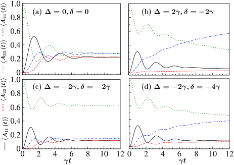
Figure 2: Time-dependent populations $\langle A_{11}(t)\rangle$ (solid-black), $\langle A_{22}(t)\rangle$ (dashed-red), $\langle A_{33}(t)\rangle$ (dots-green), and $\langle A_{44}(t)\rangle$ (dashed-dots-blue), with the atom initially in state $|3\rangle$. The parameters are: $\Omega=\gamma$ and (a) $\Delta=\delta=0$; (b) $\Delta=2\gamma$, $\delta=-2\gamma$; (c) $\Delta=\delta=-2\gamma$; (d) $\Delta=-2\gamma$, $\delta=-4\gamma$.

The remaining equations, which we omit, describe the evolution of the coherences of the $\sigma$ transitions ($\langle A_{14}\rangle$, $\langle A_{23}\rangle$) and those among the upper and lower states ($\langle A_{12}\rangle$, $\langle A_{34}\rangle$). These coherences vanish at all times because the dynamics of the $\sigma$ transitions is due only to spontaneous emission. Note, however, that for the calculation of fluorescence properties of the $\sigma$ transitions the complete set of Bloch equations, Eq.(16), is actually required.

We gain valuable information on the nontrivial dynamics of the atomic system from the single-time expectation values bypassed in the previous literature on the system. In Fig. 2, we show the populations for several particular cases, all with the atom initially in state $|3\rangle$. In the degenerate case, $\delta=0$, the upper populations reach opposite phases by the end of the first Rabi cycle, Fig. 2(a). This is understandable since the electron occupation of, say, state $|1\rangle$ implies not to be in state $|2\rangle$, and viceversa. A similar situation occurs for the lower populations. Next, we show three situations for the nondegenerate case with $\delta<0$ (as it is for ${}^{198}\mathrm{Hg}^{+}$). In Fig. 2(b) the laser is slightly detuned above the $|1\rangle-|3\rangle$ transition, but highly detuned from the $|2\rangle-|4\rangle$ transition, thus populating preferentially state $|4\rangle$ as optical pumping. In Fig. 2(c) the laser is detuned below the $|1\rangle-|3\rangle$ transition, and the $|2\rangle-|4\rangle$ transition is now on resonance with the laser, but the population is pumped mainly to state $|3\rangle$. More visible in the latter case is that the excited state populations evolve with slightly different Rabi frequencies in the nondegenerate case. In Fig. 2(d), we extend the previous case to a larger difference Zeeman splitting, such that the Rabi frequencies are equal, with the populations of the excited states again out of phase. In the next Sections, we will also consider the general cases of different Rabi frequencies and initial conditions with interesting consequences.

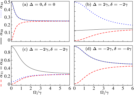
Figure 3: Steady-state populations $\alpha_{jj}$ as a function of Rabi frequency: $\alpha_{11}=\alpha_{22}$ (dashed-red), $\alpha_{33}$ (solid-black), and $\alpha_{44}$ (dots-blue). All other parameters as in Fig. 2.

In Fig. 3, we show the steady-state populations as a function of the Rabi frequency; the other parameters are the same as in Fig. 2. For strong fields, the populations tend to be equal (1/4), but arrive at that limit at different rates; for instance, for large detunings on both transitions, Fig. 3(d), it takes larger fields, as compared to the degenerate case, Fig. 3(a). On the other hand, for small detunings and weak to moderate fields, when one transition is closer to resonance than the other, the lower state of the more detuned transition is more populated, as seen in Figs. 3 (b) and (c).

IV The Scattered Field

In this Section, we study the main quantum dynamical and stationary properties of the intensity of the field scattered by the atom, with emphasis on the $\pi$ transitions. Although the intensity is not affected by interference, there are valuable insights analyzing the latter via intensity fluctuations.

IV.1 Single-Time and Stationary Properties

In principle, the reservoir and laser radiation fields are quantized. However, for free-space atom-field interactions, it is customary to simplify the theoretical description by eliminating the reservoir modes, thus obtaining the master equation for the atomic system alone, Eq. (12), and assuming the laser to be described by a classical quantity, Eq. (4), by a canonical transformation if the laser field is initially in a coherent state, and the reservoir in the vacuum state [36].

But, then, it is also customary to keep the quantum nature of the scattered field because we are interested in the quantum fluctuations of the field emitted by the source. The atom, described by a dipole operator, absorbs photons from the laser and emits them to the reservoir. The scattering process is thus mediated by the reservoir, but now the focus is on the field, whereas in the master equation, the focus is on the atom. In a procedure with the dipole and rotating-wave approximations, a relevant reservoir frequency range and field initially in the vacuum state, the scattered field is proportional to the dipole operator, so the quantum nature of the atom leaves its imprint on the reemitted field, see, e.g., Ref.[7].

The positive-frequency part of the emitted field operator is [35, 7]

$$\hat{E}^{+}(\mathbf{r},t) = \hat{E}_{\mathrm{free}}^{+}(\mathbf{r},t)+\hat{E}_{S}^{+}(\mathbf{r},\hat{t}),$$ (22)

where $\hat{E}_{\mathrm{free}}^{+}(\mathbf{r},t)$ is the free-field part which, for a reservoir in the vacuum state, does not contribute to normally ordered correlations, hence we omit it in further calculations, and

$$\hat{E}_{S}^{+}(\mathbf{r},t) = -\frac{\eta}{r}\sum_{i=1}^{4}\omega_{i}^{2}\hat{\mathbf{r}}\times(\hat{\mathbf{r}}\times\mathbf{d}_{i})S_{i}^{-}(\hat{t})$$ (23)

is the dipole source field operator in the far-field zone, where $\hat{t}=t-r/c$ is the retarded time and $\eta=(4\pi\epsilon_{0}c^{2})^{-1}$. Since $\omega_{i}\gg\gamma,\Omega,\Delta,\delta$, we may approximate the four transition as a single one $\omega_{0}$ in Eq. (23).

Making $\hat{\mathbf{r}}=\mathbf{e}_{y}$ the direction of observation and using Eq. (II) we have

$$\hat{E}_{S}^{+}(\mathbf{r},\hat{t}) = \hat{E}_{\pi}^{+}(\mathbf{r},\hat{t})\,\mathbf{e}_{z}+\hat{E}_{\sigma}^{+}(\mathbf{r},\hat{t})\,\mathbf{e}_{x},$$ (24)

i.e., the fields scattered from the $\pi$ and $\sigma$ transitions are polarized in the $\mathbf{e}_{z}$ and $\mathbf{e}_{x}$ directions, respectively, where

$$\hat{E}_{\pi}^{+}(\mathbf{r},\hat{t}) = f_{\pi}(r)\left[A_{31}(\hat{t})-A_{42}(\hat{t})\right],$$ (25a)

$$\hat{E}_{\sigma}^{+}(\mathbf{r},\hat{t}) = f_{\sigma}(r)\left[A_{32}(\hat{t})-A_{41}(\hat{t})\right],$$ (25b)

are the positive-frequency source field operators of the $\pi$ and $\sigma$ transitions, and

$$f_{\pi}(r)=-\eta\omega_{1}^{2}\mathcal{D}/\sqrt{3}r,\qquad f_{\sigma}(r)=\sqrt{2}f_{\pi}(r),$$ (26)

are their geometric factors.

The intensity in the $\pi$ transitions is given by

$$I_{\pi}(\mathbf{r},\hat{t}) = \langle\hat{E}_{\pi}^{-}(\mathbf{r},\hat{t})\cdot\hat{E}_{\pi}^{+}(\mathbf{r},\hat{t})\rangle$$ (27a)

$$= f_{\pi}^{2}(r)\langle A_{13}(\hat{t})A_{31}(\hat{t})+A_{24}(\hat{t})A_{42}(\hat{t})\rangle$$

$$= f_{\pi}^{2}(r)\langle A_{11}(\hat{t})+A_{22}(\hat{t})\rangle,$$

while in the steady state is

$$I_{\pi}^{st} = f_{\pi}^{2}(r)\left[\alpha_{11}+\alpha_{22}\right]=\frac{\Omega^{2}}{D}.$$ (27b)

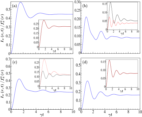
Figure 4: Fluorescence intensity (arb. units) of the $\pi$ transitions with equal initial ground state populations, $\langle A_{33}(0)\rangle=\langle A_{44}(0)\rangle=1/2$ and $\langle A_{11}(0)\rangle=\langle A_{22}(0)\rangle=0$. The other parameters are as in Fig. 2: $\Omega=\gamma$ and (a) $\Delta=\delta=0$; (b) $\Delta=2\gamma$, $\delta=-2\gamma$; (c) $\Delta=\delta=-2\gamma$; (d) $\Delta=-2\gamma$, $\delta=-4\gamma$. The insets show the populations of the excited states: $\langle A_{11}(t)\rangle$ (solid-black), $\langle A_{22}(t)\rangle$ (dashed-red).

Just adding the excited state populations with the atom initially in the single state $|3\rangle$ in Eq. (27a) gives simply $I_{\pi}(\mathbf{r},\hat{t})=f_{\pi}^{2}(r)\langle A_{11}(\hat{t})\rangle$, i.e., without the contribution of $\langle A_{22}(\hat{t})\rangle$. More interesting is the case where the initial condition is $\langle A_{33}(0)\rangle=\langle A_{44}(0)\rangle=1/2$, shown in Fig. 4 (see the populations $\langle A_{11}(t)\rangle$ and $\langle A_{22}(t)\rangle$ in the insets). The modulation in the intensity is reminiscent of the quantum beats from spontaneous decay in multilevel systems [10, 6], but with a nonzero steady state. Basically, the beats are due to the inability to tell if photons come from one $\pi$ transition or the other. The main requirement is that both ground states are initially nonzero, ideally equal [10] (see Appendix B).

Still more interesting, though, is the case of strong resonant laser and magnetic fields, $\Omega,\delta\gg\gamma$, such that the laser gets detuned somewhat far from the $|2\rangle-|4\rangle$ resonance frequency, shown in Fig. 5, with the populations $\langle A_{11}(t)\rangle$ and $\langle A_{22}(t)\rangle$ in the insets. Remarkably, beats with well-defined wave-packets are developed due to the interference of the fluorescence of both $\pi$ transitions with close Rabi frequencies, with clearly distinct average and modulation frequencies. With a larger difference Zeeman splitting, the pulsations become shorter and tend to scramble the signal.

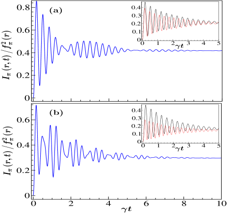
Figure 5: Fluorescence intensity (arb. units) for $\Omega=9\gamma$, $\Delta=0$, and (a) $\delta=-8\gamma$ and (b) $\delta=-15\gamma$. The insets show the excited state populations $\langle A_{11}\rangle$ (solid-black) and $\langle A_{22}\rangle$ (dotted-red). The initial conditions are $\langle A_{33}(0)\rangle=\langle A_{44}(0)\rangle=1/2$, $\langle A_{11}(0)\rangle=\langle A_{22}(0)\rangle=0$.

Save for the decay, these beats look more like those seen in introductory wave physics, described by a modulation and an average frequency, unlike the beats from spontaneous emission or weak resonance fluorescence from two or more closely separated levels. Henceforth, we (mainly) reserve the moniker beats to those due to strong applied fields. Further analyses of the beats are given in the following Sections, as they also show up in two-time correlations with particular features.

As an aside, we note that for the $\sigma$ transitions we have

$$I_{\sigma}(\mathbf{r},\hat{t}) = \langle\hat{E}_{\sigma}^{-}(\mathbf{r},\hat{t})\cdot\hat{E}_{\sigma}^{+}(\mathbf{r},\hat{t})\rangle$$ (28a)

$$= f_{\sigma}^{2}(r)[\langle A_{23}(\hat{t})A_{32}(\hat{t})+A_{14}(\hat{t})A_{41}(\hat{t})\rangle]$$

$$= f_{\sigma}^{2}(r)[\langle A_{11}(\hat{t})+A_{22}(\hat{t})\rangle],$$

$$I_{\sigma}^{st} = f_{\sigma}^{2}(r)\left[\alpha_{11}+\alpha_{22}\right],$$ (28b)

that is, also showing beats but with intensity twice that of the $\pi$ transitions, given that $f_{\sigma}^{2}(r)=2f_{\pi}^{2}(r)$.

IV.2 Intensity Fluctuations

A different angle to interference in resonance fluorescence is found by considering fluctuations of the field even though the total intensity is not affected by interference. Here, we introduce the field’s intensity in terms of atomic fluctuation operators $\Delta A_{jk}=A_{jk}-\langle A_{jk}\rangle_{st}$, such that

$$\langle A_{kl}A_{mn}\rangle = \alpha_{kl}\alpha_{mn}+\langle\Delta A_{kl}\Delta A_{mn}\rangle.$$ (29)

Only the $\pi$ transitions have nonzero coherence terms ($\alpha_{13},\alpha_{24}\neq 0$). Fluorescence in the $\sigma$ transitions is fully incoherent ($\alpha_{14}=\alpha_{23}=0$), its intensity given by Eq. (28b) so, in the remainder of this Section, we deal only with the $\pi$ transition.

From Eqs. (27b) and (29) we write the steady-state intensity in terms of products of dipole and dipole fluctuation operator expectation values,

$$I_{\pi}^{st}(\mathbf{r}) = f_{\pi}^{2}(r)\left[I_{\pi,0}^{coh}+I_{\pi,0}^{inc}+I_{\pi,cross}^{coh}+I_{\pi,cross}^{inc}\right],$$ (30)

where

$$I_{\pi,0}^{coh} = |\langle A_{13}\rangle_{st}|^{2}+|\langle A_{24}\rangle_{st}|^{2},$$ (31a)

$$I_{\pi,0}^{inc} = \langle\Delta A_{13}\Delta A_{31}\rangle+\langle\Delta A_{24}\Delta A_{42}\rangle,$$ (31b)

$$I_{\pi,cross}^{coh} = -\langle A_{13}\rangle_{st}\langle A_{42}\rangle_{st}-\langle A_{24}\rangle_{st}\langle A_{31}\rangle_{st}$$ (31c)

$$= -2\mathrm{Re}\left(\langle A_{13}\rangle_{st}\langle A_{42}\rangle_{st}\right),$$

$$I_{\pi,cross}^{inc} = -\langle\Delta A_{13}\Delta A_{42}\rangle-\langle\Delta A_{24}\Delta A_{31}\rangle$$ (31d)

$$= -2\mathrm{Re}\left(\langle\Delta A_{13}\Delta A_{42}\rangle\right).$$

Superindices $coh$ and $inc$ stand, respectively, for the coherent (depending on mean dipoles) and incoherent (depending on noise terms) parts of the emission. Subindex $0$ stands for terms with the addition of single transition products, giving the total intensity, while subindex $cross$ stands for terms with products of operators of the two $\pi$ transitions, the steady state interference part of the intensity. In terms of atomic expectation values, these intensities are:

$$I_{\pi,0}^{coh} = |\alpha_{13}|^{2}+|\alpha_{24}|^{2}$$

$$= \frac{\Omega^{2}}{4D^{2}}\left[\frac{\gamma^{2}}{2}+\Delta^{2}+(\delta-\Delta)^{2}\right],$$

$$I_{\pi,0}^{inc} = \alpha_{11}+\alpha_{22}-|\alpha_{13}|^{2}-|\alpha_{24}|^{2}$$

$$= \frac{\Omega^{2}}{D^{2}}\left[2\Omega^{2}-\frac{\gamma^{2}}{4}-\Delta^{2}-\delta^{2}\right],$$

$$I_{\pi,cross}^{coh} = -2\mathrm{Re}\left(\alpha_{13}\alpha_{42}\right)$$

$$= \frac{\Omega^{2}}{2D^{2}}\left[\frac{\gamma^{2}}{4}+\Delta(\Delta-\delta)\right],$$

$$I_{\pi,cross}^{inc} = 2\mathrm{Re}\left(\alpha_{13}\alpha_{42}\right)=-I_{\pi,cross}^{coh},$$ (32d)

The sum of these terms is, again, the total intensity, Eq. (27a). As usual in few-level resonance fluorescence, the coherent and incoherent intensities are similar only in the weak field regime, $\Omega\leq\gamma$; for strong fields, $\Omega\gg\gamma$, almost all the fluorescence is incoherent and here, in particular, $I_{\pi,0}^{inc}\gg I_{\pi,cross}^{inc}$, that is, the noninterference part becomes dominant.

IV.3 Degree of Interference - Coherent Part

In Ref. [13], a measure of the effect of interference in the coherent part of the intensity was defined as

$$I_{\pi,0}^{coh}+I_{\pi,cross}^{coh} = I_{\pi,0}^{coh}(1+C(\delta)),$$

$$C(\delta)=\frac{I_{\pi,cross}^{coh}}{I_{\pi,0}^{coh}} = \frac{\gamma^{2}/4+\Delta(\Delta-\delta)}{\gamma^{2}/4+\delta^{2}/4+(\Delta-\delta/2)^{2}},$$ (33)

independent of the Rabi frequency, shown in Fig. 6(a).

Some special cases are found analytically:

$$C(0) = 1,\qquad\delta=0,$$ (34a)

$$C(\delta_{0}) = 0,\qquad\delta_{0}=\Delta[1+(\gamma/2\Delta)^{2}],$$ (34b)

$$C(\delta_{min}) = \frac{-1}{1+\gamma^{2}/2\Delta^{2}},\qquad\delta_{min}=2\Delta[1+(\gamma/2\Delta)^{2}],$$

$$C(\delta_{1/2}^{\pm}) = 1/2,\qquad\delta_{1/2}^{\pm}=-\Delta\pm\sqrt{3\Delta^{2}+(\gamma^{2}/2)}.$$

In the degenerate case, $$C(\delta=0)=1 \delta=0 \delta C \delta_{min} \Delta^{2}\gg\gamma^{2}$$ means perfect constructive interference. That is because, at , all transitions share the same reservoir environment. Increasing the reservoir overlap decreases, and so is the interference. Negative values of indicate destructive interference; its minimum is given by . For large detunings, , we have

$$\delta_{0}=\Delta,\qquad\delta_{min}=2\Delta,\qquad\delta_{1/2}^{\pm}=-\Delta\pm\sqrt{3}\,|\Delta|.$$

We have used the special cases $\delta=\{0,\delta_{0},\delta_{min}\}$ as a guide to obtain many of the figures in this paper.

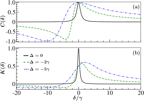
Figure 6: Relative weight of the interference terms $C(\delta)$ (a) and $K(\delta)$ (b). In (b) $\Omega=\gamma/4$. For ${}^{198}\mathrm{Hg}^{+}$, $\delta\leq 0$.

Although $C(\delta)$ is independent of Rabi frequency, it is important to recall that the coherent intensity is small in the strong laser field regime, Eqs. (32a,c), so it virtually has no role in the formation of beats.

IV.4 Degree of Interference - Incoherent Part

Likewise, we define a measure, $K(\delta)$, of the effect of interference in the intensity’s incoherent part,

$$I_{\pi,0}^{inc}+I_{\pi,cross}^{inc} = I_{\pi,0}^{inc}(1+K(\delta)),$$

$$K(\delta)=\frac{I_{\pi,cross}^{inc}}{I_{\pi,0}^{inc}} = \frac{\gamma^{2}/4+\Delta(\Delta-\delta)}{2\left[\gamma^{2}/4+\delta^{2}+\Delta^{2}-2\Omega^{2}\right]}.$$ (35)

Unlike $C(\delta)$, $K(\delta)$ also depends on the Rabi frequency as $\Omega^{-2}$, since fluctuations increase with laser intensity. Special cases are:

$$K(0) = \frac{\gamma^{2}/4+\Delta^{2}}{2\left[\gamma^{2}/4+\Delta^{2}-2\Omega^{2}\right]},\qquad\delta=0,$$ (36a)

$$K(\delta) = 0,\quad\delta=\Delta+\frac{\gamma^{2}}{4\Delta}\quad\mathrm{or}\quad\Omega\gg\gamma,\Delta,\delta.\qquad$$ (36b)

The behavior of $K(\delta)$ with $\Delta$ is more subtle. It is basically required that $\Delta\sim\Omega$ in order to preserve the shape seen in Fig. 6(b), in which case the minima for $C(\delta)$ and $K(\delta)$ are very similar. On-resonance, for example, $\Omega$ should be no larger than $0.35\gamma$. Also, we can infer that the beats are little affected by the interference term unless $\Delta\gtrsim\Omega\gg\gamma$.

V Two-Time Dipole Correlations and Power Spectrum

We have talked about the $\pi$ transitions evolving with different frequencies and the resulting quantum beats in the intensity with little quantitative analysis. The reason for delaying the analysis lies in that it is difficult to obtain general analytic solutions from the eight-equation system. Fortunately, in the strong field regime, the dressed system approach allows us to obtain very good approximate expressions, which then help us to discern the origin and positions of the peaks of the spectrum from the transitions among the dressed states [13].

The resonance fluorescence spectrum of the $J=1/2\to J=1/2$ atomic system was first considered in [11] and then very thoroughly in [12, 13]. In the strong field regime and large Zeeman splittings, a spectrum emerges with a central peak and not one [37] but two pairs of sidebands. A major result of our paper is the observation that the closeness of the side peaks makes the components interfere, causing quantum beats with well-defined mean and modulation frequencies.

The stationary Wiener-Khintchine power spectrum is given by the Fourier transform of the field autocorrelation function

$$S_{\pi}(\omega) = \mathrm{Re}\int_{0}^{\infty}d\tau e^{-i\omega\tau}\langle\hat{E}_{\pi}^{-}(0)\hat{E}_{\pi}^{+}(\tau)\rangle,$$ (37)

such that $\int_{-\infty}^{\infty}S_{\pi}(\omega)d\omega=I_{\pi}^{st}$. By writing the atomic operators in Eq. (25a) as $A_{jk}(t)=\alpha_{jk}+\Delta A_{jk}(t)$, we separate the spectrum in two parts: a coherent one,

$$S_{\pi}^{coh}(\omega) = \mathrm{Re}\int_{0}^{\infty}e^{-i\omega\tau}d\tau\left[I_{\pi,0}^{coh}+I_{\pi,cross}^{coh}\right]$$ (38)

$$= \pi\left[I_{\pi,0}^{coh}+I_{\pi,cross}^{coh}\right]\delta(\omega)$$

$$= \frac{\pi\Omega^{2}}{D^{2}}\left[\frac{\gamma^{2}}{4}+\left(\Delta-\frac{\delta}{2}\right)^{2}\right]\delta(\omega),$$

due to elastic scattering, where $I_{\pi,0}^{coh}$ and $I_{\pi,cross}^{coh}$ are given by Eqs. (32) (a) and (c), respectively; and an incoherent part,

$$S_{\pi}^{inc}(\omega) = \mathrm{Re}\int_{0}^{\infty}d\tau e^{-i\omega\tau}\langle\Delta\hat{E}_{\pi}^{-}(0)\Delta\hat{E}_{\pi}^{+}(\tau)\rangle,$$

specifically,

$$S_{\pi}^{inc}(\omega) = \mathrm{Re}\int_{0}^{\infty}d\tau e^{-i\omega\tau}\left[\langle\Delta A_{13}(0)\Delta A_{31}(\tau)\rangle\right.$$ (39)

$$+\langle\Delta A_{24}(0)\Delta A_{42}(\tau)\rangle-\langle\Delta A_{13}(0)\Delta A_{42}(\tau)\rangle$$

$$\left.-\langle\Delta A_{24}(0)\Delta A_{31}(\tau)\rangle\right],$$

due to atomic fluctuations. An outline of the numerical calculation is given in Appendix A.

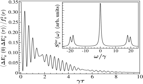
Figure 7: Dipole correlation function $\langle\Delta\hat{E}_{\pi}^{-}(0)\Delta\hat{E}_{\pi}^{+}(\tau)\rangle$ for $\Omega=9\gamma$, $\delta=-8\gamma$, and $\Delta=0$. The inset shows the corresponding incoherent spectrum $S_{\pi}^{inc}(\omega)$.

The dipole correlation $\langle\hat{E}_{\pi}^{-}(0)\hat{E}_{\pi}^{+}(\tau)\rangle$ and the corresponding incoherent spectrum in the strong driving regime and strong nondegeneracy (large $\delta$) are shown in Fig. 7. The sidebands are localized at the generalized Rabi frequencies $\pm\Omega_{1}$ and $\pm\Omega_{2}$, given by

$$\Omega_{1} = \mathcal{E}_{1}^{+}-\mathcal{E}_{1}^{-}=\sqrt{4\Omega^{2}+\Delta^{2}},$$ (40a)

$$\Omega_{2} = \mathcal{E}_{2}^{+}-\mathcal{E}_{2}^{-}=\sqrt{4\Omega^{2}+(\delta-\Delta)^{2}},$$ (40b)

where

$$\mathcal{E}_{1}^{\pm} = -\frac{\Delta}{2}\pm\frac{1}{2}\sqrt{4\Omega^{2}+\Delta^{2}},$$ (41a)

$$\mathcal{E}_{2}^{\pm} = B_{\ell}+\frac{\delta-\Delta}{2}\pm\frac{1}{2}\sqrt{4\Omega^{2}+(\delta-\Delta)^{2}},$$ (41b)

are eigenvalues of the Hamiltonian (8). Due to the spontaneous decays, these frequencies would have to be corrected, but they are very good in the relevant strong field regime. Indeed, we notice that $\Omega_{1}$ and $\Omega_{2}$ are very close to the imaginary parts of the numerical eigenvalues $\lambda_{2,3}$ and $\lambda_{4,5}$, respectively, of matrix $\mathbf{M}$, as shown in Table I.

Table 1: Eigenvalues of matrix $\mathbf{M}/\gamma$ and initial conditions of the correlations in Eq. (39) for $\Omega=9\gamma$ and $\Delta=0$.

Eigenvalues	$\delta=-8\gamma$	$\delta=-15\gamma$
$\lambda_{1}$	$-0.749386+0i$	$-0.836531+0i$
$\lambda_{2}$	$-0.583099-18.0094i$	$-0.583308-17.9981i$
$\lambda_{3}$	$-0.583099+18.0094i$	$-0.583308+17.9981i$
$\lambda_{4}$	$-0.569785-19.6808i$	$-0.5492-23.4257i$
$\lambda_{5}$	$-0.569785+19.6808i$	$-0.5492+23.4257i$
$\lambda_{6}$	$-0.5+0i$	$-0.5+0i$
$\lambda_{7}$	$-0.444846+0i$	$-0.398452+0i$
$\lambda_{8}$	$0+0i$	$0+0i$
Initial condition
$\langle\Delta A_{13}\Delta A_{31}\rangle$	$0.20836+0i$	$0.14734+0i$
$\langle\Delta A_{24}\Delta A_{42}\rangle$	$0.174014+0i$	$0.086982+0i$
$\langle\Delta A_{13}\Delta A_{42}\rangle$	$0.000134+0.002146i$	$0.000067+0.002011i$
$\langle\Delta A_{24}\Delta A_{31}\rangle$	$0.000134-0.002146i$	$0.000067-0.002011i$

The beats are the result of the superposition of waves at the frequencies $\Omega_{1}$ and $\Omega_{2}$ of the spectral sidebands, with average frequency

$$\Omega_{av}=\frac{\Omega_{2}+\Omega_{1}}{2} = \frac{\sqrt{4\Omega^{2}+(\delta-\Delta)^{2}}+\sqrt{4\Omega^{2}+\Delta^{2}}}{2},$$

and beat or modulation frequency

$$\Omega_{beat}=\frac{\Omega_{2}-\Omega_{1}}{2} = \frac{\sqrt{4\Omega^{2}+(\delta-\Delta)^{2}}-\sqrt{4\Omega^{2}+\Delta^{2}}}{2}.$$

Now, we can identify the origin of the beats in the time-dependent intensity, Eq. (27a), since the excited state populations $\langle A_{11}(t)\rangle$ and $\langle A_{22}(t)\rangle$ oscillate at the generalized Rabi frequencies $\Omega_{1}$ and $\Omega_{2}$, respectively, with initial conditions given by a nonzero superposition of the ground state populations at $t=0$. In the case of the dipole correlation $\langle\hat{E}_{\pi}^{-}(0)\hat{E}_{\pi}^{+}(\tau)\rangle$, however, the initial conditions are given in terms of products of stationary atomic expectation values (most of them the coherences $\alpha_{13},\alpha_{24}$), which become very small for $\Omega\gg\gamma$. Thus, as seen in the bottom part of Table I, the terms $\langle\Delta A_{13}(0)\Delta A_{31}(\tau)\rangle$ and $\langle\Delta A_{24}(0)\Delta A_{42}(\tau)\rangle$ are much larger than the cross terms $\langle\Delta A_{13}(0)\Delta A_{42}(\tau)\rangle$ and $\langle\Delta A_{24}(0)\Delta A_{31}(\tau)\rangle$, so the beats are basically due to the interference of those dominant terms. The strong damping of the beats, compared to those of the intensity, is due to the real eigenvalues $\lambda_{1},\lambda_{6},\lambda_{7}$. The first eigenvalue, $\lambda_{1}\sim-3\gamma/4$, in particular, is like that of the 2LA and other cases in RF. Also, if $\Delta\neq 0$ more eigenvalues would be complex, but this is an unnecessary complication in understanding the emergence of beats.

We also note that when $\delta=2\Delta$, $\Omega_{1}$ equals $\Omega_{2}$, thus the two sidebands merge into a single one, thus the beats disappear, also explaining why the populations $\langle A_{11}(\tau)\rangle$ and $\langle A_{22}(\tau)\rangle$ are out of phase, as in the degenerate case.

VI Photon-Photon Correlations

The standard method to investigate intensity fluctuations of a light source uses Brown-Twiss photon-photon correlations [24, 25]. The conditional character of this type of measurement makes it nearly free of detector inefficiencies, unlike single-detector measurements of fluorescence. This makes it one of the most used techniques in quantum optics. In Ref. [18], the effect of interference in the correlations of two photons from the $\pi$ transitions was studied, albeit only for the degenerate case and not too strong laser, finding a stronger damping of the Rabi oscillations than without interference. In this paper, we extend the photon correlations to the case of nondegenerate states. These correlations are defined as

$$g_{\pi}^{(2)}(\tau)=\frac{G_{\pi}^{(2)}(\tau)}{G_{\pi}^{(2)}(\tau\to\infty)}$$ (44)

where, using Eq. (25a) for the field operators,

$$G_{\pi}^{(2)}(\tau) = \langle\hat{E}_{\pi}^{-}(0)\hat{E}_{\pi}^{-}(\tau)\hat{E}_{\pi}^{+}(\tau)\hat{E}_{\pi}^{+}(0)\rangle$$ (45a)

$$= f_{\pi}^{4}(r)\langle[A_{13}(0)-A_{24}(0)][A_{11}(\tau)+A_{22}(\tau)]$$

$$\times[A_{31}(0)-A_{42}(0)]\rangle,$$

and

$$G_{\pi}^{(2)}(\tau\to\infty) = \left(I_{\pi}^{st}\right)^{2}=f_{\pi}^{4}(r)\left(\alpha_{11}+\alpha_{22}\right)^{2}$$ (45b)

is the normalization factor. Note that the full photon correlation, Eq.(45a), is not just the sum of the correlations of the separate $$\pi$$ transition, but it contains cross terms mixing both paths, adding to the total interference, unlike the total intensity.

The terms of the correlation obey the quantum regression formula, Eqs.(77) and (78). Then, from Eq.(91e), $G_{\pi}^{(2)}(\tau)$ is further reduced as $\langle A_{13}(0)A_{jk}(\tau)A_{42}(0)\rangle=\langle A_{24}(0)A_{jk}(\tau)A_{31}(0)\rangle=0$. We are then left with four terms,

$$G_{\pi}^{(2)}(\tau) = f_{\pi}^{4}(r)\left\{\langle A_{13}(0)[A_{11}(\tau)+A_{22}(\tau)]A_{31}(0)\rangle\right.$$ (45c)

$$\left.+\langle A_{24}(0)[A_{11}(\tau)+A_{22}(\tau)]A_{42}(0)\rangle\right\}.$$

As usual in single-atom resonance fluorescence, the correlation shows the ubiquitous, nonclassical, antibunching effect, $g_{\pi}^{(2)}(0)=0$, that is, a single atom cannot emit two photons simultaneously.

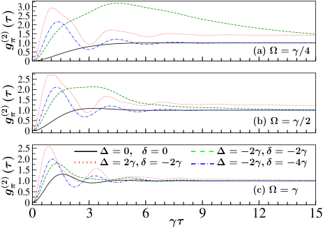
Figure 8: Photon correlations for (a) $\Omega=\gamma/4$, (b) $\Omega=\gamma/2$, and (c) $\Omega=\gamma$. The pairs of detunings ($\Delta,\delta$) are the same as those in Fig. 2.

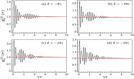
Figure 9: Photon correlations in the strong field limit, $\Omega=9\gamma$, $\Delta=0$, and large Zeeman splittings. The horizontal line helps to see that the wave packets are slightly above the long-time value $g_{\pi}^{(2)}(\infty)=1$.

Figure 8 shows $g_{\pi}^{(2)}(\tau)$ for moderately strong drivings, $\Omega=\gamma/4,\gamma/2,\gamma$, and the same sets of detunings $(\Delta,\delta)$ of Fig. 2. In the nondegenerate case, the multiple contributions and parameters cause a quite involved evolution. Notably, as seen in Fig. 2, with nonzero laser detunings, one or the other ground state traps some of the population. In $g_{\pi}^{(2)}(\tau)$ this is manifested as a slow decay and lack of oscillations (see dashed green line). This trapping effect diminishes for increasing Rabi frequency, which would cause populations to evolve more evenly among states. We will see in the next Section that the trapping effect is related to a very narrow peak in the spectra of quadratures.

Now, Fig. 9 shows the case of strong driving and large difference Zeeman splitting, $\Omega,\delta\gg\gamma$, Here, to simplify matters, we chose the atom-laser detuning $\Delta=0$. As it happens with the time-dependent populations of the excited states (Fig. 2), the dominant nonvanishing terms of $g^{(2)}(\tau)$, $\langle A_{13}(0)A_{11}(\tau)A_{31}(0)\rangle$ and $\langle A_{24}(0)A_{22}(\tau)A_{42}(0)\rangle$, evolve with close eigenvalues $\lambda_{2},\lambda_{3},\lambda_{4},\lambda_{5}$, causing quantum beats. Note the lack of strong damping from the real eigenvalues $\lambda_{1},\lambda_{6},\lambda_{7}$. Also, with initial conditions depending on the stationary populations, there is no need to prepare an initial superposition atomic state, as for beats in the intensity.

There are several effects resulting from the increase in the nondegeneracy factor $\delta$: (i) the larger number of visible wave packets; (ii) both average and beat frequencies approach one another, so the wave packets get shorter, containing very few of the fast oscillations, as seen in Fig. 9(d); and (iii) the wavepackets are initially slightly lifted above the $g^{(2)}(\tau\to\infty)=1$ value.

In the next Section, we investigate amplitude-intensity correlations, which share the main dynamical features observed in $g^{(2)}(\tau)$, with due differences in character, as the former are also analyzed in the frequency domain.

VII Quadrature Fluctuations

Quantum optics deals with the properties of the electromagnetic field. Intensity is the particle aspect of its nature, where its fluctuations are characterized by photon statistics and photon correlations. Amplitude and phase comprise the wave aspect, of which the squeezing effect is its most salient property. Squeezing is the reduction of noise in one quadrature below that of a coherent state at the expense of the other [34]. It is usually measured by balanced homodyne detection (BHD), but low quantum detector efficiency degrades the weak squeezing produced in resonance fluorescence and cavity QED systems. One alternative our group has used is conditional homodyne detection (CHD) [26, 27], which correlates a quadrature amplitude on the cue of an intensity measurement. CHD measures a third-order amplitude-intensity correlation (AIC) which, in the weak driving limit, is reduced to the second-order one, which allows for measuring squeezing, nearly free of detector inefficiencies.

While the original goal of CHD was to measure the weak squeezing in cavity QED [26, 27], it was soon realized that nonzero third-order fluctuations of the amplitude provide clear evidence of non-Gaussian fluctuations and higher-order field nonclassicality. In the present work, the fluctuations are mainly of third-order due to excitation near and above saturation, and violate classical bounds. We thus explore the phase-dependent fluctuations under conditions of quantum interference, following our recent work on CHD in resonance fluorescence [29, 30, 31].

VII.1 Quadrature Operators

To study the quadrature fluctuations, we define the field quadrature operator,

$$\hat{E}_{\pi,\phi}(\mathbf{r},\hat{t}) = \frac{1}{2}\left(E_{\pi}^{-}(\mathbf{r},\hat{t})e^{-i\phi}+E_{\pi}^{+}(\mathbf{r},\hat{t})e^{i\phi}\right)$$ (46)

$$= f_{\pi}(r)[S_{1,\phi}(\hat{t})-S_{2,\phi}(\hat{t})],$$

where $\phi$ is the phase of the local oscillator required in homodyne-type measurements, and

$$S_{1,\phi} = \frac{1}{2}\left(A_{13}e^{-i\phi}+A_{31}e^{i\phi}\right),$$ (47a)

$$S_{2,\phi} = \frac{1}{2}\left(A_{24}e^{-i\phi}+A_{42}e^{i\phi}\right).$$ (47b)

The mean quadrature field is given by

$$\langle\hat{E}_{\pi,\phi}\rangle_{st} = \frac{f_{\pi}(r)}{2}\left[\left(\alpha_{13}-\alpha_{24}\right)e^{-i\phi}+\left(\alpha_{31}-\alpha_{42}\right)e^{i\phi}\right]$$

$$= f_{\pi}(r)\mathrm{Re}\left[\left(\alpha_{13}-\alpha_{24}\right)e^{-i\phi}\right]$$

$$= f_{\pi}(r)\mathrm{Re}\left[\frac{\Omega\left(\Delta+(i\gamma-\delta)/2\right)}{D}e^{-i\phi}\right].$$

Next we rewrite $\langle\hat{E}_{\pi,\phi}\rangle_{st}$ in terms of a mean quadrature and atomic fluctuation operators $\Delta A_{jk}=A_{jk}-\langle A_{jk}\rangle_{st}$,

$$\hat{E}_{\pi,\phi}(\mathbf{r},\hat{t})=f_{\pi}(r)[\alpha_{\pi,\phi}+\Delta S_{\pi,\phi}(\hat{t})],$$ (49a)

where

$$\alpha_{\pi,\phi} = \frac{1}{2}(\alpha_{31}-\alpha_{42})e^{i\phi}+\frac{1}{2}(\alpha_{13}-\alpha_{24})e^{-i\phi},$$

$$= \mathrm{Re}\left[\frac{\Omega\left(\Delta+(i\gamma-\delta)/2\right)}{D}e^{-i\phi}\right],$$

$$\Delta S_{\pi,\phi} = \frac{1}{2}(\Delta A_{31}-\Delta A_{42})e^{i\phi}+\frac{1}{2}(\Delta A_{13}-\Delta_{24})e^{-i\phi}.$$

A similar analysis for the $\sigma$ transitions tells us that this fluorescence is fully incoherent; its mean quadrature field vanishes because $\alpha_{14}=\alpha_{23}=0$. Higher-order fluctuations, like those from the amplitude-intensity correlations are small, if any.

VII.2 Amplitude-Intensity Correlations

In CHD, a quadrature’s field $E_{\phi}$ is measured by BHD on the cue of photon countings in a separate detector. This is characterized by a correlation between the amplitude and the intensity of the field,

$$h_{\pi,\phi}(\tau)=\frac{H_{\pi,\phi}(\tau)}{H_{\pi,\phi}(\tau\to\infty)},$$ (50)

where

$$H_{\pi,\phi}(\tau) = \langle:\hat{E}_{\pi}^{-}(0)\hat{E}_{\pi}^{+}(0)\hat{E}_{\pi,\phi}(\tau):\rangle,$$ (51a)

the dots $$::$$ indicating time and normal operator orderings, and

$$H_{\pi,\phi}(\tau\to\infty) = I_{\pi}^{st}\langle E_{\pi,\phi}\rangle_{st}$$

$$= f_{\pi}^{3}(r)\left[\alpha_{11}+\alpha_{22}\right]\mathrm{Re}\left[\left(\alpha_{13}-\alpha_{24}\right)e^{-i\phi}\right]$$

$$= f_{\pi}^{3}(r)\frac{\Omega^{3}}{D^{2}}\mathrm{Re}\left[\left(\Delta+(i\gamma-\delta)/2\right)e^{-i\phi}\right]$$

is the normalization factor.

For the sake of concreteness, in this Section, we limit our discussion to the out-of-phase quadrature, $\phi=\pi/2$, which is the one that features squeezing when $\Delta=0$. We do consider, however, squeezing in the in-phase quadrature $\phi=0$ in Sect. VIII on the variance.

In several atom-laser systems $h_{\pi,\phi}(\tau)$ has been shown to be time-asymmetric [30, 31]. This is not the case with the $J=1/2\to J=1/2$ system, so we limit the analysis to positive intervals $\tau\geq 0$. Omitting the geometrical factor $f_{\pi}^{3}(r)$, which is later cancelled by normalization, we have

$$H_{\pi,\phi}(\tau) = \langle\hat{E}_{\pi}^{-}(0)\hat{E}_{\pi,\phi}(\tau)\hat{E}_{\pi}^{+}(0)\rangle$$ (52)

$$= \mathrm{Re}\left\{e^{-i\phi}\langle A_{13}(0)[A_{13}(\tau)-A_{24}(\tau)]A_{31}(0)\right.$$

$$\left.+A_{24}(0)[A_{13}(\tau)-A_{24}(\tau)]A_{42}(0)\rangle\right\}.$$

Note that $H_{\pi,\phi}(0)=0$, meaning that, like antibunching in $g^{(2)}(0)$, the atom has to build a new photon wavepacket after one has been emitted.

The AIC suggests nontrivial behavior when we take dipole fluctuations into account, that is, when the atomic operators are split into their mean plus noise, $A_{jk}=\alpha_{jk}+\Delta A_{jk}$; upon substitution in Eq. (52) we get

$$H_{\pi,\phi}(\tau) = I_{\pi}^{st}\langle E_{\pi,\phi}\rangle_{st}+H_{\pi,\phi}^{(2)}(\tau)+H_{\pi,\phi}^{(3)}(\tau),$$ (53)

or in normalized form as

$$h_{\pi,\phi}(\tau) = 1+\frac{H_{\pi,\phi}^{(2)}(\tau)}{I_{\pi}^{st}\langle E_{\pi,\phi}\rangle_{st}}+\frac{H_{\pi,\phi}^{(3)}(\tau)}{I_{\pi}^{st}\langle E_{\pi,\phi}\rangle_{st}},$$ (54)

where

$$H_{\pi,\phi}^{(2)}(\tau) = 2\mathrm{Re}\left[\langle\hat{E}_{\pi}^{+}\rangle_{st}\langle\Delta\hat{E}_{\pi}^{-}(0)\Delta\hat{E}_{\pi,\phi}(\tau)\rangle\right]$$ (55)

$$= \mathrm{Re}\left\{(\alpha_{31}-\alpha_{42})\left[\langle(\Delta A_{13}(0)-\Delta A_{24}(0)\right)\left(\Delta A_{13}(\tau)-\Delta A_{24}(\tau))\rangle e^{-i\phi}\right.\right.$$

$$\left.\left.+\langle(\Delta A_{13}(0)-\Delta A_{24}(0)\right)\left(\Delta A_{31}(\tau)\rangle-\Delta A_{42}(\tau))\rangle e^{i\phi}\right]\right\},$$

$$H_{\pi,\phi}^{(3)}(\tau) = \langle\Delta\hat{E}_{\pi}^{-}(0)\Delta\hat{E}_{\pi,\phi}(\tau)\Delta\hat{E}_{\pi}^{+}(0)\rangle$$ (56)

$$= \mathrm{Re}\left\{e^{i\phi}\langle\left[\Delta A_{13}(0)-\Delta A_{24}(0)\right]\left[\Delta A_{31}(\tau)-\Delta A_{42}(\tau)\right]\left[\Delta A_{31}(0)-\Delta A_{42}(0)\right]\rangle\right\}.$$

The initial conditions of the correlations are given in Appendix A.

From $h_{\pi,\pi/2}(0)=0$ we can obtain analytically the initial values of the second- and third-order terms,

$$h_{\pi,\pi/2}^{(2)}(0) = 1-\frac{(2\Delta-\delta)^{2}+\gamma^{2}}{2D},$$ (57)

$$h_{\pi,\pi/2}^{(3)}(0) = \frac{(2\Delta-\delta)^{2}+\gamma^{2}}{2D}-2,$$ (58)

where $D$ is given by Eq. (21).

Being the AIC a function of odd-order in the field amplitude we rightly expect a richer landscape than that of the intensity correlations, more so when one considers quantum interference. For instance, the correlation can take on not only negative values, breaking the classical bounds [26, 27]:

$$0 \leq h_{\phi}(\tau)-1\leq 1\,,$$ (59a)

$$|h_{\phi}^{(2)}(\tau)-1| \leq |h_{\phi}^{(2)}(0)-1|\leq 1\,,$$ (59b)

where the second line is valid only for weak fields such that $h_{\phi}^{(3)}(\tau)\sim 0$. These classical bounds are stronger criteria for the nonclassicality of the emitted field than squeezed light measurements, the more familiar probing of phase-dependent fluctuations. A detailed hierarchy of nonclassicality measures for higher-order correlation functions is presented in Refs. [32, 33]. In Ref. [30] an inequality was obtained that considers the full $h_{\phi}(\tau)$ by calculating the AIC for a field in a coherent state,

$$-1\leq h_{\phi}(\tau)\leq 1\,.$$ (60)

For a meaningful violation of Poisson statistics, $h_{\phi}(\tau)$ must be outside these bounds.

Also, $h_{\phi}(\tau)$ is a measure of non-Gaussian fluctuations, here of third-order in the field. Resonance fluorescence is a particularly strong case of non-Gaussian noise by being a highly nonlinear stationary nonequilibrium process [29, 30, 31, 38], thanks also to its small Hilbert space.

VII.3 Fluctuations Spectra

Since quadrature fluctuations, such as squeezing, are often studied in the frequency domain, we now define the spectrum of the amplitude-intensity correlations:

$$S_{\pi,\phi}(\omega)=8\gamma_{1}\int_{0}^{\infty}d\tau\cos{(\omega\tau)}\left[h_{\pi,\phi}(\tau)-1\right]$$ (61)

which, following Eqs. (50) and (53), can be decomposed into terms of second- and third-order in the dipole fluctuations

$$S_{\pi,\phi}^{(q)}(\omega)=8\gamma_{1}\int_{0}^{\infty}d\tau\cos{(\omega\tau)}h_{\pi,\phi}^{(q)}(\tau),$$ (62)

where $q=2,3$, so that $S_{\pi,\phi}(\omega)=S_{\pi,\phi}^{(2)}(\omega)+S_{\pi,\phi}^{(3)}(\omega)$.

As mentioned above, the AIC was devised initially to measure squeezing without the issue of imperfect detection efficiencies. Obviously, by definition, $h_{\pi,\phi}(\tau)$ and $S_{\pi,\phi}(\omega)$ are not measures of squeezing. They measure a third-order moment in the field’s amplitude, while squeezing is a second-order one in its fluctuations. The so-called spectrum of squeezing is the one for $q=2$, with the advantage for the AIC of not depending on the efficiency of detection. Squeezing is signaled by frequency intervals where $S_{\pi,\phi}^{(2)}(\omega)<0$. As a further note, the full incoherent spectrum, Eq. (V), can be obtained by adding the squeezing spectra of both quadratures [39],

$$S_{\pi}^{inc}(\omega)=\frac{1}{8\gamma_{1}}\left[S_{\pi,0}^{(2)}(\omega)+S_{\pi,\pi/2}^{(2)}(\omega)\right].$$ (63)

VII.4 Results

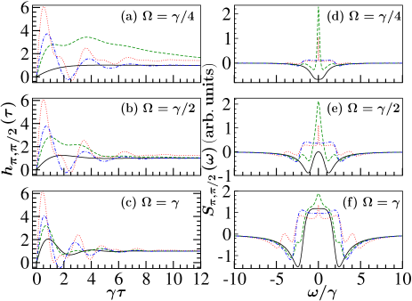
Figure 10: Amplitude-intensity correlations $h_{\pi,\phi}(\tau)$ (left panel) and corresponding spectra $S_{\pi,\phi}(\omega)$ (right panel) for the $\phi=\pi/2$ quadrature in the weak-moderate field limit. Parameters and line styles are the same as in Fig. 8: $\Delta=\delta=0$ (solid-black); $\Delta=2\gamma$ and $\delta=-2\gamma$ (dots-red); $\Delta=-2\gamma$ and $\delta=-2\gamma$ (dashed-green); $\Delta=-2\gamma$ and $\delta=-4\gamma$ (dot-dashed-blue).

We now show plots of the AICs and their spectra in Figs. 10-12 for the $\phi=\pi/2$ quadrature and the same sets of detunings $\Delta,\delta$ of Fig. 2, and weak to moderate Rabi frequencies, $\gamma/4<\Omega<\gamma$. Squeezing in the $\phi=0$ case will be considered only in the next Section. With the three parameters $\Omega$, $\Delta$, and $\delta$, there is a vast landscape of effects.

We first notice a few general features in $h_{\pi,\pi/2}(\tau)$, Fig. 10. With increasing Rabi frequencies, detunings, and Zeeman splittings, we observe the clear breakdown of the classical inequalities besides the one at $\tau=0$. Correspondingly, in the spectra, the extrema get displaced and broadened. Now, we single out the case of nondegeneracy with small detuning on the $|1\rangle-|3\rangle$ transition but large on the $|2\rangle-|4\rangle$ one, $\Delta=-\delta=2\gamma$ (green-dashed line). For weak field, $\Omega=\gamma/4$, the AIC decays very slowly, with a corresponding very narrow spectral peak. The slow decay is also clearly visible in the photon correlation, Fig. 8a. As we mentioned in Sect. III regarding Fig. 2b, state $|4\rangle$ ends up with a large portion of the steady-state population due to optical pumping; not quite a trapping state, so there is no electron shelving per se, as argued in [13]. This effect is washed out for larger Rabi frequencies, allowing for faster recycling of the populations. To a lesser degree, slow decay and sharp peak occur for opposite signs of $\Delta$ and $\delta$.

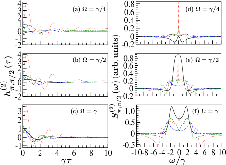
Figure 11: Second-order component of the AIC, $h_{\pi,\phi}^{(2)}(\tau)$ (left panel), and corresponding (squeezing) spectra, $S_{\pi,\phi}^{(2)}(\omega)$ (right panel), with the same parameters and line styles as in Fig. 10.

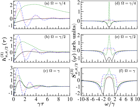
Figure 12: Third-order component of the AIC, $h_{\pi,\phi}^{(3)}(\tau)$ (left panel), and corresponding spectra, $S_{\pi,\phi}^{(3)}(\omega)$ (right panel), with the same parameters and line styles as in Fig. 10.

Splitting the AIC and spectra into components of second- and third-order fluctuations, Figs. 11 and 12, respectively, help us better understand the quadrature fluctuations. For $\Omega\ll\gamma$ and $\Delta=\delta=0,$ the squeezing spectrum is a negative central peak centered at $\omega=0$ (not shown). $\Omega=\gamma/4$ is already a strong enough driving that the squeezing gets displaced to sidebands and eventually gets lost (positive) for stronger fields. Finite laser and Zeeman detunings are detrimental to squeezing unless larger $\Omega$ is applied. For increasing Rabi frequencies, in $h_{\pi,\pi/2}^{(2)}(\tau)$ there is a reduction in amplitudes and nonclassicality except for the case of opposite signs of detuning and difference Zeeman splitting. Note that the sharp spectral peak in the latter case takes up most of the corresponding peak in Fig. 10. Increasing $\Omega$, the fluorescent emission becomes more incoherent, Eqs.(32), and third-order fluctuations overcome the second-order ones. Also, comparing Figs. 11 and 12 we see that $h_{\phi}^{(3)}(\tau)$ is mainly responsible for the breakdown of the classical bounds. Moreover, we see that the slow-decay–sharp-peak is mostly a third-order effect.

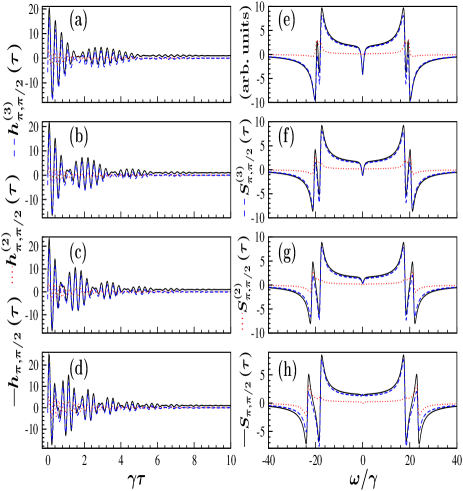
Figure 13: Second-order (dots-red), third-order (dashed-blue), and total (solid-black) AICs (left panel) and corresponding spectra (right panel) for $\Omega=9\gamma$, $\Delta=0$, and: (a,e) $\delta=-8\gamma$, (b,f) $\delta=-10\gamma$, (c,g) $\delta=-12\gamma$, (d,h) $\delta=-15\gamma$.

For very strong fields and large Zeeman splittings, $\Omega,|\delta|\gg\gamma$, Fig. 13, the AIC shows beats as in the photon correlations. Unlike those in $g^{(2)}(\tau)$, the wavepackets here oscillate around $h(\tau)=1$. The spectral peaks are localized around the Rabi frequencies $\pm\Omega_{1},\pm\Omega_{2}$ in a dispersive manner, revealing the wave character of the quadratures.

Studies of the spectrum of squeezing for the $J=1/2-J=1/2$ system were reported in [17], choosing to increase $\Omega_{1},\Omega_{2}$ with large detunings, $\Delta>\Omega$, showing two close negative sidebands. In these conditions, beats would also occur but are not reported. The authors do, nonetheless, notice the interesting case where, for $\delta=2\Delta$, $\Omega_{1}$ and $\Omega_{2}$ are equal, so the two sidebands merge into a single one. In this case, the beats would disappear.

An odd-order function of the field amplitude opens the door naturally to probe for non-Gaussian fluctuations, the AIC reaching non-zero third-order moments, $\langle\Delta A_{ij}\Delta A_{kl}\Delta A_{mn}\rangle$. The latter are very small when the driving is weak, and the emission is mainly coherent but, as we saw above, they dominate for strong driving, and the emission is mostly incoherent. A few-level system, such as the $J=1/2-J=1/2$ one, is strongly nonlinear, so non-Gaussian fluctuations of its resonance fluorescence are ubiquitous. With the AIC, unlike moments in photon counting, which are positive-definite, the fluctuations can also take negative values and break classical bounds of quadratures in both time and frequency domains [29, 31]. Quantum beats, a major signature of interference, are found to be also non-Gaussian in resonance fluorescence, as shown particularly in Fig. 13.

VIII Variance

The variance is a measure of the total noise in a quadrature; it is defined as

$$V_{\phi} = \langle:(\Delta E_{\phi})^{2}:\rangle=\mathrm{Re}\left[e^{-i\phi}\langle\Delta\hat{E}^{-}\Delta\hat{E}_{\phi}\rangle_{st}\right],$$ (64)

and is related to the spectrum of squeezing as

$$V_{\phi} = \frac{1}{4\pi\gamma\eta}\int_{-\infty}^{\infty}d\omega S_{\phi}^{(2)}(\omega).$$ (65)

where $\eta$ is the detector efficiency. The maximum value of $V_{\phi}$ is 1/4, obtained when there is very strong driving, when almost all the emitted light is incoherent. Negative values of the variance are a signature of squeezing but, unlike the quadrature spectra, the squeezing is the total one in the field, independent of frequency.

For the $\pi$ transitions we have

$$V_{\pi,\phi} = \frac{f_{\pi}^{2}(r)}{2}\mathrm{Re}\left[-(\alpha_{13}-\alpha_{24})^{2}e^{-2i\phi}\right.$$

$$\left.+(\alpha_{11}+\alpha_{22}-|\alpha_{13}-\alpha_{24}|^{2})\right]$$

$$= \frac{f_{\pi}^{2}(r)}{2}\frac{\Omega^{2}}{D}\left[1-\frac{[(2\Delta-\delta)\cos{\phi}+\gamma\sin{\phi}]^{2}}{2D}\right].$$

For $\phi=\pi/2$ and $\phi=0$ we have

$$V_{\pi,\pi/2} = \frac{f_{\pi}^{2}(r)}{2}\frac{\Omega^{2}}{D}\left[1-\frac{\gamma^{2}}{2D}\right],$$ (67a)

$$V_{\pi,0} = \frac{f_{\pi}^{2}(r)}{2}\frac{\Omega^{2}}{D}\left[1-\frac{(2\Delta-\delta)^{2}}{2D}\right],$$ (67b)

respectively, where $D$ is given by Eq. (21).

In Fig. 14 we plot the variances of the out-of-phase $\phi=\pi/2$ (left panel) and in-phase $\phi=0$ (right panel) quadratures. The interplay of parameters is a complex one, but we mostly use the ones of previous figures. For $\phi=\pi/2$, as usual in single-atom resonance fluorescence systems, squeezing is restricted to small Rabi frequencies; increasing laser and Zeeman detunings are detrimental to squeezing. In contrast, for $\phi=0$ nonzero laser or Zeeman detunings are necessary to produce squeezing, with a strong dependence on their sign: on-resonance (not shown), there is no squeezing, a result also known for a two-level atom; in Fig. 14(d) the laser is tuned below the $|1\rangle-|3\rangle$ transition, $\Delta=-2\gamma$, and there is no squeezing (positive variance), but the variance is reduced for large $\delta$; in Fig. 14(e) the laser is tuned above that transition, $\Delta=2\gamma$, and there is squeezing for not very large Rabi frequencies. Large values of $\delta$ tend to reduce the variance, be it positive or negative.

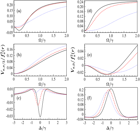
Figure 14: Variance of the quadratures of the fluorescence of the $\pi$ transitions: left panel for $\phi=\pi/2$ and right panel for $\phi=0$. (a,b,d,e) as a function of Rabi frequency and (c,f) as a function of laser detuning. In all cases, $\delta=0$ is given by a solid-black line, and $\delta=-0.5\gamma$ by a dashed-red line; the dotted-blue line is $\delta=-2\gamma$ in (a,b,d,e) and $\delta=-\gamma$ in (c,f). Additionally, (a) $\Delta=0$, (b) $\Delta=-2\gamma$, (c) $\Omega=0.2\gamma$, (d) $\Delta=-2\gamma$, (e) $\Delta=2\gamma$, (f) $\Omega=0.8\gamma$.

VIII.1 Out-of-phase quadrature

We now discuss a complementary view of the variance. For $\phi=\pi/2$ we can identify the Rabi frequency interval within which squeezing takes place,

$$0<\Omega<\frac{1}{2}\sqrt{\gamma^{2}/2-\delta^{2}/2-2(\Delta-\delta/2)^{2}},$$ (68)

and the Rabi frequency for maximum squeezing is

$$\tilde{\Omega}_{\pi/2}=\frac{1}{2}\sqrt{\frac{\gamma^{4}/2-2[(\delta-\Delta)^{2}+\Delta^{2}]^{2}}{3\gamma^{2}+2[(\delta-\Delta)^{2}+\Delta^{2}]^{2}}}.$$ (69)

Thus, the variance at $\tilde{\Omega}_{\pi/2}$ is

$$V_{\pi,\pi/2}^{(\tilde{\Omega}_{\pi/2})}(\Delta=0,\delta) = \frac{f_{\pi}^{2}(r)}{16}\frac{(\gamma^{4}/2-2\delta^{4})(\delta^{2}-\gamma^{2})}{\gamma^{2}(\gamma^{2}+2\delta^{2})(\delta^{2}+\gamma^{2})},$$

for $$\Delta=0 |\delta/\gamma|<1/\sqrt{2}$$ and ;

$$V_{\pi,\pi/2}^{(\tilde{\Omega}_{\pi/2})}(\Delta,\delta=0) = \frac{f_{\pi}^{2}(r)}{16}\frac{(\gamma^{4}/2-8\Delta^{4})(4\Delta^{2}-\gamma^{2})}{\gamma^{2}(\gamma^{2}+4\Delta^{2})^{2}},$$

for $$\delta=0 |\Delta/\gamma|<1/\sqrt{2} \Delta=\delta=0$$ and ; and the maximum total squeezing is obtained at ,

$$V_{\pi,\pi/2}^{(\tilde{\Omega}_{\pi/2})}(0,0) = -\frac{f_{\pi}^{2}(r)}{32},\qquad\tilde{\Omega}_{\pi/2}=\frac{\gamma}{2\sqrt{6}}.$$ (70c)

For $\phi=\pi/2$ squeezing is limited to elliptical regions of weak driving and small detunings $\Delta$ and $\delta$:

$$2\delta^{2}+8\Omega^{2} < \gamma^{2},\qquad\Delta=0,$$ (71a)

$$4\Delta^{2}+8\Omega^{2} < \gamma^{2},\qquad\delta=0.$$ (71b)

These results indicate that the conditions for squeezing in the resonance fluorescence of the $J=1/2-J=1/2$ system are more stringent than that for a two-level atom [29]: it is limited to smaller Rabi frequencies and the minimum variance is also smaller. Hence, there is no net squeezing in the regime of quantum beats seen in the previous Sections.

VIII.2 In-phase quadrature

For $\phi=0$, squeezing is obtained in the Rabi frequency interval, for $\delta=0$,

$$0<\Omega<\frac{1}{\sqrt{2}}\sqrt{\Delta^{2}-\gamma^{2}/4},\qquad|\Delta|>\gamma/2,$$ (72)

with maximum squeezing at the Rabi frequency

$$\tilde{\Omega}_{0}=\frac{1}{2\sqrt{2}}\sqrt{\frac{16\Delta^{2}-\gamma^{2}}{12\Delta^{2}+\gamma^{2}}},$$ (73)

requiring finite detuning from both $\pi$ transitions ($\Delta\neq 0$) and stronger driving, $\Omega\sim\gamma$ [see Fig. 14(d)-14(f)].

Thus, the variance at $\tilde{\Omega}_{0}$ is

$$V_{\pi,0}^{(\tilde{\Omega}_{0})}(\delta) = -\frac{f_{\pi}^{2}(r)}{128}\frac{4\Delta^{2}-\gamma^{2}}{\Delta^{2}(4\Delta^{2}+\gamma^{2})},\quad|\Delta|\geq\gamma/2.$$ (74)

This expression gets the asymptotic value

$$\lim_{\Delta\to\infty}V_{\pi,0}^{(\tilde{\Omega}_{0})} = -\frac{f_{\pi}^{2}(r)}{32},$$ (75)

which is the same as that for the $\pi/2$ quadrature. The region for squeezing obeys the relation

$$4\Delta^{2}-8\Omega^{2}<\gamma^{2}.$$ (76)

So, to obtain squeezing in this quadrature, it is necessary to have detunings $\Delta>\gamma/4$ for any Rabi frequency.

IX Conclusions

We have studied interference effects on the resonance fluorescence of the $\pi$ transitions in a $J=1/2-J=1/2$ angular momentum atomic system driven by a linearly polarized laser field and a magnetic field to lift the level degeneracies. These fields make the transition frequencies unequal, so the $\pi$ transitions evolve with different generalized Rabi frequencies, which we observed first in the time-dependent populations of the excited states and whose interference produces quantum beats. When the atom is subject to large laser and magnetic fields, the beats have well-defined modulation of the fast oscillations. We studied beats in the total intensity and two-time correlations. It is generally found that the main contributions to these observables come from the interference of the individual $\pi$ transitions density probabilities, while those due to vacuum-induced coherence, which link both transition amplitudes, have a lesser role. This is because the upper levels are very separated due to the large ac and Zeeman splittings.

Nonclassical features of the fluorescence light are shown in photon correlations, such as antibunching, $g^{(2)}(0)=0$, and in amplitude-intensity correlations, with squeezing and violation of classical inequalities, Eqs. (59, 60). In resonance fluorescence, interference is generally detrimental to squeezing, even at moderate laser and magnetic fields. In the regime of well-defined beats, there is squeezing near the effective Rabi frequencies but not in the total noise, as the variance confirms. Also, in this regime, third-order fluctuations in the field quadrature amplitude dominate over the second-order ones and break classical inequalities, making the fluctuations strongly non-Gaussian, making the beats and their spectra outstanding features. Resonance fluorescence, being a highly nonequilibrium and nonlinear stationary process, is a useful laboratory for the study of nonclassical and non-Gaussian fluctuations. The AIC, with its conditional character (based on recording only pairs of events) and third-order moments in the field amplitudes, provides a practical and proven alternative to more recent work based on time-gating photodetection [40] and higher odd-order moments in photoncounting [41, 42].

So far, few quantum interference experiments have been performed on the $J=1/2-J^{\prime}=1/2$ system, but we believe experiments to observe our results are within reach. Certainly, single-atom resonance fluorescence is bound to both photon collection and detection inefficiencies. Conditional measurements such as photon-photon and photon-quadrature correlations solve this issue; also, through (inverse) Fourier transform of the spectrum might be an efficient way to observe beats. However, both laser-atom and Zeeman detunings should not be too large since they imply reduced fluorescence rates $\gamma_{1}(\alpha_{11}+\alpha_{22})$, see Eq.(20a), which may be detrimental in measurements. Also, a large difference Zeeman splitting means that the upper levels would be very separated, diminishing the vacuum-induced coherence. The beats would be better observed if $\Delta\leq\gamma$ and $\delta$ of just several $\gamma$ in the strong field regime, $\Omega\gg\gamma$. In this regime, the beats are due basically to interference among the incoherently coupled waves of the two $\pi$ transitions, but bound by the $\sigma$ transitions. Finally, we have used interference to mean not only the presence of cross-terms as in Young-type interference but also the superposition of coupled transitions as discussed in this paper.

X Acknowledgments.

The authors thank Dr. Ricardo Román-Ancheyta for continued interest in this work and Dr. Irán Ramos-Prieto for useful comments at an early stage of the project. ADAV thanks CONACYT, Mexico, for the support of scholarship No. 804318.

ORCID numbers: Héctor M. Castro-Beltrán https://orcid.org/0000-0002-3400-7652, Octavio de los Santos-Sánchez https://orcid.org/0000-0002-4316-0114, Luis Gutiérrez https://orcid.org/0000-0002-5144-4782, Alan D. Alcantar-Vidal https://orcid.org/0000-0003-3849-7844.

Appendix A Time-Dependent Solutions of the Matrix Equations and Spectra by Formal Integration of Correlations

The two-time photon correlations under study have the general form $\langle\mathbf{W}(\tau)\rangle=\langle O_{1}(0)\mathbf{R}(\tau)O_{2}(0)\rangle$, where $\mathbf{R}$ is the Bloch vector and $O_{1,2}$ are system operators. The same applies to correlations of fluctuation operators $\Delta\mathbf{R},\,\Delta O_{1,2}$. Using the quantum regression formula [7], the correlations obey the equation

$$\langle\dot{\mathbf{W}}(\tau)\rangle=\mathbf{M}\langle\mathbf{W}(\tau)\rangle,$$ (77)

which has the formal solution

$$\langle\mathbf{W}(\tau)\rangle=e^{\mathbf{M}\tau}\langle\mathbf{W}(0)\rangle,$$ (78)

where $\mathbf{M}$ is given by

$$\mathbf{M}=\left(\begin{array}[]{cccccccc}-\gamma&-i\Omega&0&0&i\Omega&0&0&0\\ -i\Omega&-\left(\frac{\gamma}{2}+i\Delta\right)&0&0&0&i\Omega&0&0\\ 0&0&-\gamma&i\Omega&0&0&-i\Omega&0\\ 0&0&i\Omega&-\left(\frac{\gamma}{2}+i(\Delta-\delta)\right)&0&0&0&-i\Omega\\ i\Omega&0&0&0&-\left(\frac{\gamma}{2}-i\Delta\right)&-i\Omega&0&0\\ \gamma_{1}&i\Omega&\gamma_{\sigma}&0&-i\Omega&0&0&0\\ 0&0&-i\Omega&0&0&0&-\left(\frac{\gamma}{2}-i(\Delta-\delta)\right)&i\Omega\\ \gamma_{\sigma}&0&\gamma_{2}&-i\Omega&0&0&i\Omega&0\end{array}\right).$$ (87)

Also, the spectra of stationary systems can be evaluated more effectively using the above formal approach. Be $g(\tau)=\langle\mathbf{W}(\tau)\rangle$. Then, a spectrum is calculated as

$$S(\omega) \propto \int_{0}^{\infty}\cos{\omega\tau}\,g(\tau)\,d\tau=\int_{0}^{\infty}\cos{\omega\tau}\,e^{\mathbf{M}\tau}g(0)\,d\tau$$ (88)

$$= \mathrm{Re}\int_{0}^{\infty}e^{-(i\omega\mathbf{1}-\mathbf{M})\tau}g(0)\,d\tau$$

$$= \mathrm{Re}\left[(i\omega\mathbf{1}-\mathbf{M})^{-1}g(0)\right],$$

where $\mathbf{1}$ is the identity matrix. For example, the incoherent spectrum requires calculations of the type

$$S^{inc}(\omega) = \mathrm{Re}\int_{0}^{\infty}d\tau e^{-i\omega\tau}e^{\mathbf{M}\tau}\langle\Delta A_{ij}(0)\Delta A_{kl}(0)\rangle_{st}$$ (89)

$$= \mathrm{Re}\left[(\mathbf{M}-i\omega\mathbf{1})^{-1}\langle\Delta A_{ij}(0)\Delta A_{kl}(0)\rangle_{st}\right].\qquad$$

For the initial conditions of the correlations we use the following operator products and correlations in compact form:

$$A_{kl}A_{mn} = A_{kn}\delta_{lm}\,,$$ (90a)

$$\langle A_{kl}A_{mn}\rangle = \alpha_{kn}\delta_{lm},$$ (90b)

$$A_{ij}A_{kl}A_{mn} = A_{in}\delta_{jk}\delta_{lm},$$ (90c)

$$\langle A_{ij}A_{kl}A_{mn}\rangle = \alpha_{in}\delta_{jk}\delta_{lm}.$$ (90d)

Hence, the relevant initial conditions are:

$$\langle A_{13}\mathbf{R}\rangle = \left(0,0,0,0,\alpha_{11},\alpha_{13},0,0\right)^{T},$$ (91a)

$$\langle A_{24}\mathbf{R}\rangle = \left(0,0,0,0,0,0,\alpha_{22},\alpha_{24}\right)^{T},$$ (91b)

$$\langle A_{13}\mathbf{R}A_{31}\rangle = \left(0,0,0,0,0,\alpha_{11},0,0\right)^{T},$$ (91c)

$$\langle A_{24}\mathbf{R}A_{42}\rangle = \left(0,0,0,0,0,0,0,\alpha_{22}\right)^{T},$$ (91d)

$$\langle A_{13}\mathbf{R}A_{42}\rangle = \langle A_{24}\mathbf{R}A_{31}\rangle=0,$$ (91e)

where $\mathbf{R}=\left(A_{11},A_{13},A_{22},A_{24},A_{31},A_{33},A_{42},A_{44}\right)^{T}$ is the Bloch vector. For correlations with fluctuation operator products, $\Delta A_{ij}=A_{ij}-\alpha_{ij}$, we have

$$\langle\Delta A_{kl}\Delta A_{mn}\rangle = \alpha_{kn}\delta_{lm}-\alpha_{kl}\alpha_{mn},$$ (92)

$$\langle\Delta A_{ij}\Delta A_{kl}\Delta A_{mn}\rangle = \alpha_{in}\delta_{lm}\delta_{jk}-\alpha_{il}\alpha_{mn}\delta_{jk}$$ (93)

$$-\alpha_{in}\alpha_{kl}\delta_{jm}-\alpha_{ij}\alpha_{kn}\delta_{lm}$$

$$+2\alpha_{ij}\alpha_{kl}\alpha_{mn}.$$

Now, recalling that $\alpha_{12}=\alpha_{14}=\alpha_{23}=\alpha_{34}=0$, we write the detailed initial conditions of the correlations (Bloch equations and quantum regression formula):

$$\langle\Delta A_{13}\Delta\mathbf{R}\rangle = \left(-\alpha_{13}\alpha_{11},\,-\alpha_{13}^{2},\,-\alpha_{13}\alpha_{22},\,-\alpha_{13}\alpha_{24},\,\alpha_{11}-|\alpha_{13}|^{2},\,\alpha_{13}-\alpha_{13}\alpha_{33},\,-\alpha_{13}\alpha_{42},\,-\alpha_{13}\alpha_{44}\right)^{T}\,,\qquad$$ (94a)

$$\langle\Delta A_{24}\Delta\mathbf{R}\rangle = \left(-\alpha_{24}\alpha_{11},\,-\alpha_{24}\alpha_{13},\,-\alpha_{24}\alpha_{22},\,-\alpha_{24}^{2},\,-\alpha_{24}\alpha_{31},\,-\alpha_{24}\alpha_{33},\,\alpha_{22}-|\alpha_{24}|^{2},\,\alpha_{24}-\alpha_{24}\alpha_{44}\right)^{T},\qquad$$ (94b)

$$\langle\Delta A_{13}\Delta\mathbf{R}\Delta A_{31}\rangle = \left(2|\alpha_{13}|^{2}\alpha_{11}-\alpha_{11}^{2},\,2|\alpha_{13}|^{2}\alpha_{13}-2\alpha_{11}\alpha_{13},\right.$$ (94c)

$$\left.2|\alpha_{13}|^{2}\alpha_{22}-\alpha_{11}\alpha_{22},\,2|\alpha_{13}|^{2}\alpha_{24}-\alpha_{11}\alpha_{24},\right.$$

$$\left.2|\alpha_{13}|^{2}\alpha_{31}-2\alpha_{11}\alpha_{31},\,2|\alpha_{13}|^{2}\alpha_{33}+\alpha_{11}-2|\alpha_{13}|^{2}-\alpha_{11}\alpha_{33},\right.$$

$$\left.2|\alpha_{13}|^{2}\alpha_{42}-2\alpha_{11}\alpha_{42},\,2|\alpha_{13}|^{2}\alpha_{44}-\alpha_{11}\alpha_{44}\right)^{T}.$$

$$\langle\Delta A_{24}\Delta\mathbf{R}\Delta A_{42}\rangle = \left(2|\alpha_{24}|^{2}\alpha_{11}-\alpha_{11}\alpha_{22},\,2|\alpha_{24}|^{2}\alpha_{13}-\alpha_{22}\alpha_{13},\right.$$ (94d)

$$\left.2|\alpha_{24}|^{2}\alpha_{22}-\alpha_{22}^{2},\,2|\alpha_{24}|^{2}\alpha_{24}-2\alpha_{22}\alpha_{24},\right.$$

$$\left.2|\alpha_{24}|^{2}\alpha_{31}-\alpha_{22}\alpha_{31},\,2|\alpha_{24}|^{2}\alpha_{33}-\alpha_{22}\alpha_{33},\right.$$

$$\left.2|\alpha_{24}|^{2}\alpha_{42}-2\alpha_{22}\alpha_{42},\,2|\alpha_{24}|^{2}\alpha_{44}+\alpha_{22}-2|\alpha_{24}|^{2}-\alpha_{22}\alpha_{44}\right)^{T}.$$

$$\langle\Delta A_{13}\Delta\mathbf{R}\Delta A_{42}\rangle = \left(2\alpha_{13}\alpha_{11}\alpha_{42},\,2\alpha_{13}^{2}\alpha_{42},\,2\alpha_{13}\alpha_{22}\alpha_{42},\,(2|\alpha_{24}|^{2}-\alpha_{22})\alpha_{13},\right.$$ (94e)

$$\left.(2|\alpha_{13}|^{2}-\alpha_{11})\alpha_{42},\,(2\alpha_{13}\alpha_{33}-\alpha_{13})\alpha_{42},\,2\alpha_{13}\alpha_{42}^{2},\,(2\alpha_{13}\alpha_{44}-\alpha_{13})\alpha_{42}\right)^{T},$$

$$\langle\Delta A_{24}\Delta\mathbf{R}\Delta A_{31}\rangle = \left(2\alpha_{24}\alpha_{11}\alpha_{31},\,(2|\alpha_{13}|^{2}-\alpha_{11})\alpha_{24},\,2\alpha_{24}\alpha_{22}\alpha_{31},\,2\alpha_{24}^{2}\alpha_{31},\right.$$ (94f)

$$\left.2\alpha_{24}\alpha_{31}^{2},\,(2\alpha_{24}\alpha_{33}-\alpha_{24})\alpha_{31},\,(2|\alpha_{24}|^{2}-\alpha_{22})\alpha_{31},\,(2\alpha_{24}\alpha_{44}-\alpha_{24})\alpha_{31}\right)^{T}.$$

Appendix B Condition for Optimal Appearance of Beats in the Intensity

We consider a simplified, unitary, model to estimate the optimal initial population of the ground states to make well-formed beats. First, we diagonalize the Hamiltonian Eq. (8). The eigenvalues and eigenstates are

$$\mathcal{E}_{1}^{\pm} = -\frac{\Delta}{2}\pm\frac{1}{2}\sqrt{4\Omega^{2}+\Delta^{2}},$$ (95a)

$$\mathcal{E}_{2}^{\pm} = B_{\ell}+\frac{\delta-\Delta}{2}\pm\frac{1}{2}\sqrt{4\Omega^{2}+(\delta-\Delta)^{2}},$$ (95b)

and

$$|u_{1}\rangle = \sin{\Theta_{1}}|1\rangle+\cos{\Theta_{1}}|3\rangle,$$

$$|u_{2}\rangle = -\cos{\Theta_{1}}|1\rangle+\sin{\Theta_{1}}|3\rangle,$$

$$|u_{3}\rangle = \sin{\Theta_{2}}|2\rangle+\cos{\Theta_{2}}|4\rangle,$$

$$|u_{4}\rangle = -\cos{\Theta_{2}}|2\rangle+\sin{\Theta_{2}}|4\rangle,$$ (96)

respectively, where

$$\sin{\Theta_{1}} = \frac{2\Omega}{\sqrt{\left(\Delta+\sqrt{\Delta^{2}+4\Omega^{2}}\right)^{2}+4\Omega^{2}}},$$

$$\cos{\Theta_{1}} = \frac{\Delta+\sqrt{\Delta^{2}+4\Omega^{2}}}{\sqrt{\left(\Delta+\sqrt{\Delta^{2}+4\Omega^{2}}\right)^{2}+4\Omega^{2}}},$$

$$\sin{\Theta_{2}} = \frac{2\Omega}{\sqrt{\left((\delta-\Delta)+\sqrt{(\delta-\Delta)^{2}+4\Omega^{2}}\right)^{2}+4\Omega^{2}}},$$

$$\cos{\Theta_{2}} = \frac{(\delta-\Delta)+\sqrt{(\delta-\Delta)^{2}+4\Omega^{2}}}{\sqrt{\left((\delta-\Delta)+\sqrt{(\delta-\Delta)^{2}+4\Omega^{2}}\right)^{2}+4\Omega^{2}}}.$$

It is now straightforward to obtain the excited-state populations. If the initial state of the system is $\rho(0)=\langle A_{33}(0)\rangle|3\rangle\langle 3|+\langle A_{44}(0)\rangle|4\rangle\langle 4|$ we get

$$\langle A_{33}(t)\rangle = \frac{1}{2}\langle A_{33}(0)\rangle\sin^{2}{(2\Theta_{1})}(1-\cos{(\Omega_{1}t)}),\qquad$$ (98a)

$$\langle A_{44}(t)\rangle = \frac{1}{2}\langle A_{44}(0)\rangle\sin^{2}{(2\Theta_{2})}(1-\cos{(\Omega_{2}t)}),\qquad$$ (98b)

and the intensity of the field is

$$\frac{I_{\pi}(\mathbf{r},t)}{f_{\pi}^{2}(r)} = \langle A_{33}(0)\rangle\sin^{2}{(2\Theta_{1})}+A_{44}(0)\rangle\sin^{2}{(2\Theta_{2})}$$ (99)

$$-\langle A_{33}(0)\rangle\sin^{2}{(2\Theta_{1})}\cos{(\Omega_{1}t)}$$

$$-\langle A_{44}(0)\rangle\sin^{2}{(2\Theta_{2})}\cos{(\Omega_{2}t)}.$$

A necessary condition for the beating behavior to occur is that the initial ground-state populations are both nonvanishing in the nondegenerate case. Now, assuming the relation

$$\frac{\langle A_{33}(0)\rangle}{\langle A_{44}(0)\rangle}=\frac{\sin^{2}{(2\Theta_{2})}}{\sin^{2}{(2\Theta_{1})}}$$ (100)

is satisfied by choosing appropriate parameter values $(\Omega,\delta,\Delta)$ for given values of initial ground state populations we would get

$$I_{\pi}(\mathbf{r},t) = f_{\pi}^{2}(r)\langle A_{33}(0)\rangle\sin^{2}{(2\Theta_{1})}$$ (101)

$$\times\left[1-\cos{(\Omega_{beat}t)}\cos{(\Omega_{av}t)}\right],$$

where $\Omega_{beat}=(\Omega_{2}-\Omega_{1})/2$ and $\Omega_{av}=(\Omega_{2}+\Omega_{1})/2$.

References

• [1] D. G. Norris, L. A. Orozco, P. Barberis-Blostein, and H. J. Carmichael, Phys. Rev. Lett. 105, 123602 (2010).
• [2] A. D. Cimmarusti, C. A. Schroeder, B. D. Patterson, L. A. Orozco, P. Barberis-Blostein, and H. J. Carmichael, New J. Phys. 15, 013017 (2013).
• [3] A. Zajonc, Phys. Lett. 96A, 61 (1983).
• [4] A. Lee, H. S. Han, F. K. Fatemi, S. L. Rolston, and K. Sinha, Phys. Rev. A 107, 013701 (2023).
• [5] Z. Wu, J. Li, and Y. Wu, Phys. Rev. A 108, 023727 (2023).
• [6] Z. Ficek and S. Swain, Quantum Interference and Coherence: Theory and Experiments (Springer, New York, 2005).
• [7] H. J. Carmichael, Statistical Methods in Quantum Optics 1: Master Equations and Fokker-Planck Equations (Springer-Verlag, Berlin, 2002).
• [8] H. J. Metcalf and P. van der Straten, Laser Cooling and Trapping (Springer-Verlag, Berlin, 1999).
• [9] D. Budker, D. F. Kimball, and D. P. DeMille, Atomic Physics: Exploration Through Problems and Solutions, 2nd. Ed. (Oxford University Press, Oxford, 2008).
• [10] Z. Ficek and S. Swain, Phys. Rev. A 69, 023401 (2004).
• [11] D. Polder and M. F. H. Schuurmans, Phys. Rev. A 14, 1468 (1976).
• [12] M. Kiffner, J. Evers, and C. H. Keitel, Phys. Rev. Lett. 96, 100403 (2006).
• [13] M. Kiffner, J. Evers, and C. H. Keitel, Phys. Rev. A 73, 063814 (2006).
• [14] M. Kiffner, M. Macovei, J. Evers, and C. H. Keitel, in Progress in Optics, E. Wolf, ed. 55, 85 (Elsevier, Amsterdam, 2010).
• [15] U. Eichmann, J. C. Bergquist, J. J. Bollinger, J. M. Gilligan, W. M. Itano, D. J. Wineland, and M. G. Raizen, Phys. Rev. Lett. 70, 2359 (1993).
• [16] M. Fischer, B. Srivathsan, L. Alber, M. Weber, M. Sonderman, and G. Leuchs, Appl. Phys. B: Lasers and Optics, 123, 48 (2017).
• [17] H.-T. Tan, H.-X. Xia, and G.-X. Li, J. Phys. B: At. Mol. Opt. Phys., 42, 125502 (2009).
• [18] S. Das and G. S. Agarwal, Phys. Rev. A 77, 033850 (2008).
• [19] H.-B. Zhang, S.-P. Wu, and G.-X. Li, Phys. Rev. A 102, 053717 (2020).
• [20] S. Wolf, S. Richter, J. von Zanthier, and F. Schmidt-Kaler, Phys. Rev. Lett. 124, 063603 (2020).
• [21] M. Jakob and J. Bergou, Phys. Rev. A 60, 4179 (1999).
• [22] H. B. Crispin and R. Arun, J. Phys. B: At. Mol. Opt. Phys., 52, 075402 (2019).
• [23] H. B. Crispin and R. Arun, J. Phys. B: At. Mol. Opt. Phys., 53, 055402 (2020).
• [24] R. Hanbury-Brown and R. Q. Twiss, Nature 177, 27 (1956).
• [25] R. J. Glauber, Phys. Rev. Lett. 10, 84 (1963).
• [26] H. J. Carmichael, H. M. Castro-Beltran, G. T. Foster, and L. A. Orozco, Phys. Rev. Lett. 85, 1855 (2000).
• [27] G. T. Foster, L. A. Orozco, H. M. Castro-Beltran, and H. J. Carmichael, Phys. Rev. Lett. 85, 3149 (2000).
• [28] A. T. Forrester, R. A. Gudmunsen, and P. O. Johnson, Phys. Rev. 99, 1691 (1955).
• [29] H. M. Castro-Beltrán, R. Román-Ancheyta, and L. Gutiérrez, Phys. Rev. A 93, 033801 (2016).
• [30] L. Gutiérrez, H. M. Castro-Beltrán, R. Román-Ancheyta, and L. Horvath, J. Opt. Soc. Am. B 34, 2301 (2017).
• [31] O. de los Santos-Sánchez and H. M. Castro-Beltrán, J. Phys. B: At. Mol. Opt. Phys. 54, 055002 (2021).
• [32] E. V. Shchukin and W. Vogel, Phys. Rev. A 72, 043808 (2005).
• [33] E. V. Shchukin and W. Vogel, Phys. Rev. Lett. 96, 200403 (2006).
• [34] D. F. Walls and G J. Milburn, Quantum Optics, 2nd. Ed. (Springer-Verlag, Berlin, 2008).
• [35] G. S. Agarwal, Quantum Statistical Theories of Spontaneous Emission and their Relation to Other Approaches (Springer-Verlag, Berlin, 1974).
• [36] B. R. Mollow, Phys. Rev. A 12, 1919 (1975).
• [37] B. R. Mollow, Phys. Rev. 188, 1969 (1969).
• [38] Q. Xu, E. Greplova, B. Julsgaard, and K. Mølmer, Phys. Scripta, 90, 128004 (2015).
• [39] P. R. Rice and H. J. Carmichael, J. Opt. Soc. Am. B 5, 1661 (1988).
• [40] T. Sonoyama, K. Takahashi, B. Charoensombutamon, S. Takasu, K. Hattori, D. Fukuda, K. Fukui, K. Takase, W. Asavanant, J. Yoshikawa, M. Endo, and A. Furusawa, Phys. Rev. Res. 5, 033156 (2023).
• [41] Y.-X. Wang and A. A. Clerk, Phys. Rev. Res. 2, 033196 (2020).
• [42] M. Sifft and D. Hägele, Phys. Rev. A 107, 052203 (2023).