Thermodynamic Correlation Inequality

Abstract

Trade-off relations place fundamental limits on the operations that physical systems can perform. This Letter presents a trade-off relation that bounds the correlation function, which measures the relationship between a system’s current and future states, in Markov processes. The obtained bound, referred to as the thermodynamic correlation inequality, states that the change in the correlation function has an upper bound comprising the dynamical activity, a thermodynamic measure of the activity of a Markov process. Moreover, by applying the obtained relation to the linear response function, it is demonstrated that the effect of perturbation can be bounded from above by the dynamical activity.

Introduction.— Trade-off relations imply that there are impossibilities in the physical world that cannot be overcome by technological advances. The most well-known example is the Heisenberg uncertainty relation [1, 2], which establishes a limit on the precision of position-momentum measurement. The quantum speed limit is interpreted as an energy-time trade-off relation and places a limit on the speed at which the quantum state can be changed [3, 4, 5, 6, 7, 8, 9, 10] (see [11] for a review). It has many applications in quantum computation [12], quantum communication [13, 14], and quantum thermodynamics [5]. Recently, the concept of speed limit has also been considered in classical systems [15, 16, 17]. In particular, the Wasserstein distance can be used to obtain the minimum entropy production required for a stochastic process to transform one probability distribution into another [18, 19, 20, 21, 22]. Moreover, the speed limit has been generalized to the time evolution of the observables [23, 24, 25, 26, 27]. A related principle, known as the thermodynamic uncertainty relation, was recently proposed in stochastic thermodynamics [28, 29, 30, 31, 32, 33, 34, 35, 36, 37, 38, 39, 40, 41, 42, 43, 44, 45, 46, 47, 48, 49, 50] (see [51] for a review). This principle states that, for thermodynamic systems, higher accuracy can be achieved at the expense of higher thermodynamic costs. Recently, thermodynamic uncertainty relations have become a central topic in nonequilibrium thermodynamics; furthermore, their importance is also recognized from a practical standpoint because thermodynamic uncertainty relations can be used to infer entropy production without detailed knowledge of the system [52, 53, 54, 55].

This Letter presents a trade-off relation that confers bounds for the correlation function in Markov processes. The correlation function is a statistical measure that quantifies the correlation between the current state of a system and its future or past states. In a Markov process, the correlation function can be used to analyze the dependence of the current state on past states, and to identify any patterns in the system’s behavior over time. The correlation function provides spectral information through the Wiener-Khinchin theorem and plays a fundamental role in linear response theory [56]. Considering the significant role of the correlation function in stochastic processes, it is crucial to clearly illustrate its relationship with other physical quantities. We derive the thermodynamic correlation inequality, stating that the amount of correlation change has an upper bound that comprises the dynamical activity, which quantifies the activity of a system of interest. The derivation presented herein is based on considering the time evolution in a scaled path probability space [57], which can be regarded as a realization of bulk-boundary correspondence in Markov processes. By applying the Hölder inequality and a recently derived relation [57], the upper bound for the correlation function [Eq. (5)] is obtained. The obtained bound exhibits unexpected generality; it holds for any Markov process with an arbitrary time-independent transition rate and can be generalized to multipoint correlation functions. The linear response function can be represented by the time derivative of the corresponding correlation function, as stated by the fluctuation–dissipation theorem. Upper bounds to the perturbation applied to the system are derived by applying the thermodynamic correlation inequality to the linear response function.

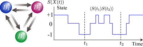
Figure 1: Markov process with three states $\{B_{1},B_{2},B_{3}\}$. In this example, we are interested in the correlation $\braket{S(t_{1})S(t_{2})}$, where the score function $S(B_{\nu})$ is specified by $S(B_{1})=-1$, $S(B_{2})=0$, and $S(B_{3})=1$.

Results.—The thermodynamic correlation inequality is derived for a Markov process. Consider a Markov process with $N$ states, $\mathcal{B}\equiv\{B_{1},B_{2},\cdots,B_{N}\}$. Let $\{X(t)|t\geq 0\}$ be a collection of discrete random variables that take values in $\mathcal{B}$ (that is $X(t)\in\mathcal{B}$). Let $P(\nu;t)$ be the probability that $X(t)$ is $B_{\nu}$ at time $t$ and $W_{\nu\mu}$ be the transition rate of $X(t)$ from $B_{\mu}$ to $B_{\nu}$. The time evolution of $\mathbf{P}(t)\equiv[P(1;t),\ldots,P(N;t)]^{\top}$ is governed by the following master equation:

$$\frac{d\mathbf{P}(t)}{dt}=\mathbf{W}\mathbf{P}(t),$$ (1)

where $\mathbf{W}\equiv\{W_{\nu\mu}\}$ and diagonal elements are defined as $W_{\nu\nu}\equiv-\sum_{\mu(\neq\nu)}W_{\mu\nu}$. Next, we define a score function $S(B_{\nu})$ that takes a state $B_{\nu}$ ($\nu\in\{1,2,\ldots,N\}$) and returns a real value of $(-\infty,\infty)$. Moreover, we define

$$S_{\mathrm{max}}\equiv\max_{B\in\mathcal{B}}|S(B)|,$$ (2)

which is the maximum absolute value of the score function within $\mathcal{B}$. We also define another score function $T(B_{\nu})$ similar to $S(B_{\nu})$ and define $T_{\mathrm{max}}$ analogously. When it is clear from the context, we express $S(t)\equiv S(X(t))$ or $T(t)\equiv T(X(t))$ for simplicity. The correlation function $C(t)\equiv\braket{S(0)T(t)}$ is of interest, where

$$\braket{S(0)T(t)} =\sum_{\mu,\nu}T(B_{\nu})S(B_{\mu})P(\mu;0)P(\nu;t|\mu;0)$$

$$=\mathds{1}\mathbf{T}e^{\mathbf{W}t}\mathbf{S}\mathbf{P}(0).$$ (3)

Here, $P(\nu;t|\mu;0)$ is the conditional probability that $X(t)=B_{\nu}$ given $X(0)=B_{\mu}$, $\mathds{1}\equiv[1,1,\ldots,1]$ is the trace state, $\mathbf{S}\equiv\mathrm{diag}[S(B_{1}),\ldots,S(B_{N})]$, and $\mathbf{T}\equiv\mathrm{diag}[T(B_{1}),\ldots,T(B_{N})]$. The correlation function $C(t)$ has been extensively explored in the field of stochastic processes [58, 59]. Recently, the correlation function was considered in the context of the quantum speed limit [26, 60], which was obtained as a particular case of the speed limits on observables. As an example of a classical system, a trichotomous process comprising three states $\mathcal{B}=\{B_{1},B_{2},B_{3}\}$ is shown in Fig. 1. $X(t)$ in this process exhibits random switching between $B_{1}$, $B_{2}$, and $B_{3}$. For a trichotomous process, the score function is typically given by $S(B_{1})=-1$, $S(B_{2})=0$, and $S(B_{3})=1$. To quantify the Markov process, we define the time-integrated dynamical activity $\mathcal{A}(t)$ as follows [61]:

$$\mathcal{A}(t)\equiv\int_{0}^{t}dt^{\prime}\sum_{\nu,\mu,\nu\neq\mu}P(\mu;t^{\prime})W_{\nu\mu}.$$ (4)

$\mathcal{A}(t)$ represents the average number of jumps during the interval $[0,t]$, and it quantifies the activity of the stochastic process. The dynamical activity plays a fundamental role in classical speed limits [15] and thermodynamic uncertainty relations [30, 32].

In the Markov process, we obtain the upper bound of the correlation function $C(t)$. For $0\leq t_{1}<t_{2}$, we obtain the following bound:

$$\left|C(t_{1})-C(t_{2})\right|\leq 2S_{\mathrm{max}}T_{\mathrm{max}}\sin\left[\frac{1}{2}\int_{t_{1}}^{t_{2}}\frac{\sqrt{\mathcal{A}(t)}}{t}dt\right],$$ (5)

which holds for $0\leq\frac{1}{2}\int_{t_{1}}^{t_{2}}\frac{\sqrt{\mathcal{A}(t)}}{t}dt\leq\frac{\pi}{2}$. For $t_{1}$ and $t_{2}$ outside this range, the upper bound is $\left|C(t_{1})-C(t_{2})\right|\leq 2S_{\mathrm{max}}T_{\mathrm{max}}$, which trivially holds true. Equation (5) is the thermodynamic correlation inequality and is the main result of this Letter. Note that all the quantities in Eq. (5) can be physically interpreted. A sketch of the proof of Eq. (5) is provided near the end of this Letter. Equation (5) holds for an arbitrary time-independent Markov process that starts from an arbitrary initial probability distribution with arbitrary score functions $S(B_{\nu})$ and $T(B_{\nu})$. Equation (5) states that higher dynamical activity allows the system to forget its current state quickly, which is in agreement with the intuitive notion. In stochastic thermodynamics, entropy production plays a central role in thermodynamic inequalities. Entropy production measures the extent of irreversibility of a Markov process, whereas dynamical activity quantifies its intrinsic time scale. Moreover, entropy production is not well defined for Markov processes that include irreversible transitions. By contrast, dynamical activity can be defined for any Markov process. This makes it particularly suitable for the correlation function, which needs to be calculated for any given Markov process. A weaker bound can be obtained by using the thermodynamic uncertainty relation derived in a previous study [57] (see Ref. [62] for details). Let us consider particular cases of Eq. (5). Taking $t_{1}=0$ and $t_{2}=t$ with $t>0$, Eq. (5) provides the upper bound for $|C(0)-C(t)|$:

$$\left|C(0)-C(t)\right|\leq 2S_{\mathrm{max}}T_{\mathrm{max}}\sin\left[\frac{1}{2}\int_{0}^{t}\frac{\sqrt{\mathcal{A}(t^{\prime})}}{t^{\prime}}dt^{\prime}\right],$$ (6)

where $0\leq\frac{1}{2}\int_{0}^{t}\frac{\sqrt{\mathcal{A}(t^{\prime})}}{t^{\prime}}dt^{\prime}\leq\frac{\pi}{2}$ (the saturating conditions are presented in Ref. [62]). Moreover, let $\epsilon$ be an infinitesimally small positive value. Substituting $t_{1}=t-\epsilon$ and $t_{2}=t$ into Eq. (5) and using the Taylor expansion for the sinusoidal function, we obtain

$$\left|\frac{dC(t)}{dt}\right|\leq\frac{S_{\mathrm{max}}T_{\mathrm{max}}\sqrt{\mathcal{A}(t)}}{t}.$$ (7)

Equation (7) states that the absolute change of the correlation function is determined by the dynamical activity. For $t\to 0$, the right side of Eq. (7) diverges to infinity. However, the derivative of $C(t)$ at $t=0$, represented as $\left|\partial_{t}C(t)\right|_{t=0}=\left|\mathds{1}\mathbf{T}\mathbf{W}\mathbf{S}\mathbf{P}(0)\right|$, is finite. This implies that the upper bound of Eq. (7) is not tight as $t$ approaches $0$.

As an intermediate step in the derivation of Eq. (6), the following inequality holds:

$$\left|C(0)-C(t)\right|\leq 2S_{\mathrm{max}}T_{\mathrm{max}}\sqrt{1-\eta(t)},$$ (8)

where $\eta(t)$ is the Bhattacharyya coefficient between the path probabilities within $[0,t]$ having the transition rate matrix $\mathbf{W}$ and the null transition rate matrix $\mathbf{W}=0$. Since $\sqrt{1-\eta(t)}\leq\sin\left[(1/2)\int_{0}^{t}\sqrt{\mathcal{A}\left(t^{\prime}\right)}/t^{\prime}\,dt^{\prime}\right]$, Eq. (8) is tighter than Eq. (6). The inequality of Eq. (8) holds for any value of $t$ because the Bhattacharyya coefficient is always bounded between $0$ and $1$. $\eta(t)$ can be computed as $\eta(t)\equiv\left(\sum_{\mu}P(\mu;0)\sqrt{e^{-t\sum_{\nu(\neq\mu)}W_{\nu\mu}}}\right)^{2}$, which can be represented by quantities of the Markov process [62]. Note that $\eta(t)$ constitutes a lower bound in thermodynamic uncertainty relations [69]. The term within the square root in $\eta(t)$ represents the survival probability that there is no jump starting from $B_{\mu}$. Therefore, when the activity of the dynamics is lower, the survival probability increases and, in turn, $\eta(t)$ yields a higher value. Although $\eta(t)$ has fewer physical interpretations than dynamical activity $\mathcal{A}(t)$, it has an advantage over Eq. (6) that the bound of Eq. (8) holds for any value of $t$.

Now, we comment on possible improvements and generalizations to the thermodynamic correlation inequality. The inequality can be tightened by replacing $S_{\mathrm{max}}T_{\mathrm{max}}$, included in Eq. (5), with $\frac{1}{2}\left[\max_{B_{1},B_{2}\in\mathcal{B}}S(B_{1})T(B_{2})-\min_{B_{1},B_{2}\in\mathcal{B}}S(B_{1})T(B_{2})\right]$. In addition, it is also possible to consider the $J$-point correlation function ($J\geq 2$ is an integer), which serves as a generalization of the two-point correlation function discussed above. The results are presented in detail in Ref. [62].

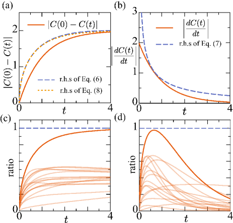
Figure 2: (a) $|C(0)-C(t)|$ as a function $t$ for the two-state Markov process, which is shown by the solid line. Its two upper bounds, the right-hand sides of Eqs. (6) and (8), are depicted by dashed and dotted lines, respectively. (b) $|\partial_{t}C(t)|$ as a function $t$ for the two-state Markov process and its upper bound, which are shown by the solid and dashed lines, respectively. In the two-state Markov process in (a) and (b), the transition rate is $W_{12}=1$ and $W_{22}=-1$ ($0$ for the other entries), the initial distribution is $\mathbf{P}(0)=[0,1]^{\top}$, and the score function is $S(B_{1})=-1$, $S(B_{2})=1$, $T(B_{1})=-1$, and $T(B_{2})=1$. (c) Ratio $|C(0)-C(t)|/\left(2S_{\mathrm{max}}T_{\mathrm{max}}\sin\left[(1/2)\int_{0}^{t}\sqrt{\mathcal{A}\left(t^{\prime}\right)}/t^{\prime}\,dt^{\prime}\right]\right)$ as a function of $t$. The light solid lines are random realizations, whereas the dark solid line corresponds to the setting of (a). (d) Ratio $\left|\partial_{t}C(t)\right|/\left(S_{\mathrm{max}}T_{\mathrm{max}}\sqrt{\mathcal{A}(t)}/t\right)$ as a function of $t$. The light solid lines are random realizations and the dark solid line corresponds to the setting of (b). In (c) and (d), the ratios must not exceed $1$, which is depicted by the dashed lines. For the random realizations in (c) and (d), we randomly determine the transition rate $\mathbf{W}$, the initial probability $\mathbf{P}(0)$, and the score function $S(B_{\nu})$ for $N=2,3,4$, where we use $T(B_{\nu})=S(B_{\nu})$ for $T(B_{\nu})$.

We perform numerical simulations to validate Eqs. (6)–(8). We prepare a two-state Markov process ($\mathcal{B}=\{B_{1},B_{2}\}$) and plot $|C(0)-C(t)|$ and $|\partial_{t}C(t)|$ as functions of $t$ in Figs. 2(a) and (b), respectively, by the solid lines (see the caption of Fig. 2 for details). In Fig. 2(a), we plot the right-hand sides of Eqs. (6) and (8), which are upper bounds of $|C(0)-C(t)|$, by the dashed and dotted lines, respectively. Furthermore, we plot the right-hand side of Eq. (7), the upper bound of $|\partial_{t}C(t)|$, by the dashed line in Fig. 2(b). From Fig. 2(a), we observe that Eq. (6) provides an accurate estimate of the upper bound. In this case, the difference between the two upper bounds given by Eqs. (6) and (8) is negligible. The upper bound shown in Fig. 2(b) becomes less tight for a large $t$, because the decay of the upper bound is approximately $O(t^{-1/2})$ whereas the correlation function decays exponentially in this model. Next, we randomly generate Markov processes and verify whether the bounds hold for the random realizations (see the caption of Fig. 2 for details). We calculate the ratio, the left-hand sides divided by the right-hand sides of Eqs. (6) and (7), in Figs. 2(c) and (d), respectively, by the light solid lines. The ratio should not exceed $1$, as indicated by the dashed lines. In Figs. 2(c) and (d), the dark solid lines correspond to the results shown in Figs. 2(a) and (b), respectively. All realizations are below $1$, which numerically verifies the bounds.

Linear response.—The correlation function $C(t)$ is closely related to linear response theory [56]. The correlation bounds in Eqs. (6) and (7) are applied to the linear response theory [62]. Suppose that a Markov process is in the steady state $\mathbf{P}_{st}=[P_{st}(1),\ldots,P_{st}(N)]^{\top}$, which satisfies $\mathbf{W}\mathbf{P}_{st}=0$. A weak perturbation $\chi\mathbf{F}f(t)$ is applied to the master equation in Eq. (1), which is $\mathbf{W}\to\mathbf{W}+\chi\mathbf{F}f(t)$ in Eq. (1). Here, $\chi$ denotes the perturbation strength satisfying $0<|\chi|\ll 1$, $\mathbf{F}$ is an $N\times N$ matrix, and $f(t)$ is arbitrary real function of time $t$. The probability distribution is expanded as $\mathbf{P}(t)=\mathbf{P}_{st}+\chi\mathbf{P}_{1}(t)$, where $\mathbf{P}_{1}(t)$ is the first-order correction to the probability distribution. By collecting the first-order contribution $O(\chi)$ in Eq. (1), $\mathbf{P}_{1}(t)$ is given by [62]

$$\mathbf{P}_{1}(t)=\int_{-\infty}^{t}e^{\mathbf{W}(t-t^{\prime})}\mathbf{F}\mathbf{P}_{st}f(t^{\prime})dt^{\prime}.$$ (9)

Let a score function $G(B_{\nu})$ be considered. Define the expectation of $G(B_{\nu})$ as $\braket{G}=\sum_{\nu}G(B_{\nu})P(\nu;t)=\mathds{1}\mathbf{G}\mathbf{P}(t)$, where $\mathbf{G}\equiv\mathrm{diag}[G(B_{1}),\ldots,G(B_{N})]$. The change in $\braket{G}$ due to the perturbation, represented by $\Delta G\equiv\mathds{1}\mathbf{G}\mathbf{P}(t)-\mathds{1}\mathbf{G}\mathbf{P}_{st}$, is $\Delta G(t)=\chi\int_{-\infty}^{\infty}R_{G}(t-t^{\prime})f(t^{\prime})dt^{\prime}$, where $R_{G}(t)$ denotes the linear response function:

$$R_{G}(t)=\begin{cases}\mathds{1}\mathbf{G}e^{\mathbf{W}t}\mathbf{F}\mathbf{P}_{st}&t\geq 0\\ 0&t<0\end{cases}.$$ (10)

In the linear response regime, any input-output relation can be expressed through $R_{G}(t)$. From Eq. (3), the time derivative of $C(t)$ is $\partial_{t}C(t)=\mathds{1}\mathbf{T}e^{\mathbf{W}t}\mathbf{W}\mathbf{S}\mathbf{P}_{st}$. Comparing Eq. (10) and $\partial_{t}C(t)$, when $\mathbf{G}=\mathbf{T}$ and $\mathbf{F}=\mathbf{W}\mathbf{S}$, then $\partial_{t}C(t)$ provides the linear response function of Eq. (10), which is the statement of the fluctuation-dissipation theorem.

As a particular case, let us consider the pulse perturbation $f(t)=\delta(t)$, where $\delta(t)$ is the Dirac delta function. This perturbation corresponds to the application of a sharp pulsatile perturbation at $t=0$. Then the change in the expectation of $T(B_{\nu})$ under the perturbation $\mathbf{F}=\mathbf{W}\mathbf{S}$, represented by $\Delta T^{(p)}$, is $\Delta T^{(p)}(t)=\chi\partial_{t}C(t)$ (the superscript (p) represents that it is the pulse response). The correlation bound in Eq. (7) yields

$$\left|\Delta T^{(p)}(t)\right|\leq\chi S_{\mathrm{max}}T_{\mathrm{max}}\sqrt{\frac{\mathfrak{a}}{t}}\,\,\,\,(t>0),$$ (11)

where $\mathfrak{a}$ is the dynamical activity $\mathfrak{a}\equiv\sum_{\nu,\mu,\nu\neq\mu}P_{st}(\mu)W_{\nu\mu}$ (note that $\mathcal{A}(t)=\mathfrak{a}t$ for the steady state). Equation (11) relates the dynamical activity to the effect of the pulse perturbation in the Markov process. The step response can be calculated similarly. We apply a constant perturbation switched on at $t=0$, which can be modeled by $f(t)=\Theta(t)$ with $\Theta(t)$ being the Heaviside step function. We obtain $\Delta T^{(s)}(t)=\chi\int_{0}^{t}R_{T}(t^{\prime})dt^{\prime}=\chi\left(C(t)-C(0)\right)$, which along with Eq. (6) yields the following bound:

$$|\Delta S^{(s)}(t)|\leq 2\chi S_{\mathrm{max}}T_{\mathrm{max}}\sin\left[\sqrt{\mathfrak{a}t}\right]\,\,\,\,(t>0).$$ (12)

Equation (12) holds for $0\leq\sqrt{\mathfrak{a}t}\leq\pi/2$. For $t$ outside this range, the trivial inequality $|\Delta S^{(s)}(t)|\leq 2\chi S_{\mathrm{max}}T_{\mathrm{max}}$ holds true.

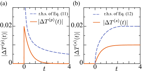
Figure 3: (a) Response under the pulse perturbation, where the solid line denotes $\Delta T^{(p)}(t)$ as a function of $t$ and the dashed line shows its upper bound [the right-hand side of Eq. (11)]. (b) Response under the step perturbation, where the solid line denotes $\Delta T^{(s)}(t)$ as a function of $t$ and the dashed line shows its upper bound [the right-hand side of Eq. (12)]. In (a) and (b), the transition matrix is $W_{12}=W_{21}=1$ (the diagonal elements are $W_{11}=W_{22}=-1$), and the score functions are $S(B_{1})=-1$, $S(B_{2})=1$, $T(B_{1})=-1$, and $T(B_{2})=1$. Additionally, the perturbation strength $\chi$ is set to $0.01$.

We perform numerical simulations to validate Eqs. (11) and (12). We prepare a two-state Markov process ($\mathcal{B}=\{B_{1},B_{2}\}$) and plot $|\Delta T^{(p)}(t)|$ and $|\Delta T^{(s)}(t)|$ as functions of $t$ in Figs. 3(a) and (b), respectively, by the solid lines (see the caption of Fig. 3 for details). We plot their upper bounds by the dashed lines. From Figs. 3(a) and (b), we can observe that the bounds are satisfied for both systems. As $t$ increases, the upper bound loosens in Fig. 3(a). This is because the upper bound decays at $O(t^{-1/2})$, whereas the decay rate of $|\Delta T^{(p)}(t)|$ is exponential. In Fig. 3(b), at $t=4$, there is a two-fold gap between the bound and $\Delta T^{(s)}(t)$; however, if the bound is halved, the bound is invalid.

Conclusion.—This letter presents the relation between the correlation function and dynamical activity in the Markov process. The obtained bounds hold for an arbitrary time-independent transition rate starting from an arbitrary initial distribution. By applying the obtained bounds to the linear response theory, we demonstrated that the effect of perturbations on a steady-state system is bounded by the dynamical activity. The findings herein can potentially enhance our understanding of nonequilibrium dynamics, as the correlation function plays a fundamental role in thermodynamics.

Appendix: Derivation.—Here, we provide a sketch of proof of Eqs. (5) and (8). For details of the derivation, refer to Ref. [62].

Let $p(x;t)$ be the general probability distribution of $x$ at time $t$ ($x$ is an arbitrary random variable). Let $F(x)$ be an observable of $x$ and $\braket{F}_{t}\equiv\sum_{x}F(x)p(x;t)$ be the expectation of $F(x)$ at time $t$. From the Hölder inequality, the following relation holds:

$$\left|\braket{F}_{t_{1}}-\braket{F}_{t_{2}}\right|\leq 2F_{\max}\mathrm{TVD}\left(p(x;t_{1}),p(x;t_{2})\right),$$ (13)

where $F_{\max}\equiv\max_{x}|F(x)|$ and $\mathrm{TVD}(\cdot,\cdot)$ is the total variation distance:

$$\mathrm{TVD}(p(x;t_{1}),p(x;t_{2}))\equiv\frac{1}{2}\sum_{x}|p(x;t_{1})-p(x;t_{2})|.$$ (14)

The speed limit relations are conventionally concerned with the time evolution of $\mathbf{P}(t)$. In contrast, we consider the time evolution of the path probability in Eq. (13), which was previously studied [57]. The final time $\tau>0$ of the Markov process is first fixed. Let $\omega_{t}\equiv[X(t^{\prime})]_{t^{\prime}=0}^{t^{\prime}=t}$ be the trajectory of a Markov process within the time interval $[0,t]$ ($0\leq t\leq\tau$) and let $\mathcal{P}(\omega_{t};\mathbf{W})$ be the path probability (path integral) with the transition rate $\mathbf{W}$. We can not substitute $\mathcal{P}(\omega_{t};\mathbf{W})$ into Eq. (13) because the size of $\omega_{t}$ is different for different $t$. Therefore, we introduce the scaled process [57]:

$$\mathcal{Q}(\omega_{\tau};t)\equiv\mathcal{P}\left(\omega_{\tau};\frac{t}{\tau}\mathbf{W}\right).$$ (15)

In Eq. (15), $\mathcal{Q}(\omega_{\tau};t)$ is the path probability of “scaled” process; the scaled process is the same as the original process, except for its time scale. In the scaled process, the transition rate is $(t/\tau)\mathbf{W}$, which is $t/\tau$ times faster than the original process. Therefore, the information at time $t$ in the original process with the transition rate $\mathbf{W}$ can be obtained at time $\tau$ in the scaled process with the transition rate $(t/\tau)\mathbf{W}$. The total variation distance admits the following upper bound:

$$\mathrm{TVD}(\mathcal{Q}(\omega_{\tau};t_{1}),\mathcal{Q}(\omega_{\tau};t_{2}))$$

$$\leq\sqrt{1-\mathrm{Bhat}(\mathcal{Q}(\omega_{\tau};t_{1}),\mathcal{Q}(\omega_{\tau};t_{2}))^{2}}.$$ (16)

Using the results of Ref. [57], the following relation holds for $0\leq t_{1}<t_{2}\leq\tau$:

$$\frac{1}{2}\int_{t_{1}}^{t_{2}}\frac{\sqrt{\mathcal{A}(t)}}{t}dt\geq\arccos\mathrm{Bhat}\left(\mathcal{Q}\left(\omega_{\tau};t_{1}\right),\mathcal{Q}\left(\omega_{\tau};t_{2}\right)\right).$$ (17)

Substituting Eq. (17) into Eq. (16), we obtain

$$\mathrm{TVD}\left(\mathcal{Q}(\omega_{\tau};t_{1}),\mathcal{Q}(\omega_{\tau};t_{2})\right)\leq\sin\left[\frac{1}{2}\int_{t_{1}}^{t_{2}}\frac{\sqrt{\mathcal{A}(t)}}{t}dt\right].$$ (18)

Consider an observable $\mathcal{C}(\omega_{\tau})$, defined as

$$\mathcal{C}(\omega_{\tau})\equiv S(X(0))T(X(\tau)).$$ (19)

Then the expectation of $\mathcal{C}(\omega_{\tau})$ with respect to $\mathcal{Q}(\omega_{\tau};t)$ yields the correlation, i.e., $\braket{\mathcal{C}(\omega_{\tau})}_{t}\equiv\sum_{\omega_{\tau}}\mathcal{Q}(\omega_{\tau};t)\mathcal{C}(\omega_{\tau})=\braket{S(X(0))T(X(t))}$. Combining Eqs. (13) and (18), and considering $\mathcal{C}(\omega_{\tau})$ for the observable in Eq. (13), we obtain

$$\left|\braket{\mathcal{C}}_{t_{1}}-\braket{\mathcal{C}}_{t_{2}}\right|\leq 2\mathcal{C}_{\max}\sin\left[\frac{1}{2}\int_{t_{1}}^{t_{2}}\frac{\sqrt{\mathcal{A}(t)}}{t}dt\right],$$ (20)

which leads to the main result of Eq. (5).

Let us derive the bound of Eq. (8), which can be obtained as an intermediate step in the above derivation. Instead of using Eq. (18) for deriving the bound, we employ Eq. (16) with $t_{1}=0$ and $t_{2}=\tau$. The Bhattacharyya coefficient yields $\mathrm{Bhat}\left(\mathcal{Q}\left(\omega_{\tau};0\right),\mathcal{Q}\left(\omega_{\tau};\tau\right)\right)=\sum_{\mu}P(\mu;0)\sqrt{e^{-\tau\sum_{\nu(\neq\mu)}W_{\nu\mu}}}$ (see Ref. [62] for details), which provides the bound in Eq. (8).