One-Loop Electron Mass and QED Trace Anomaly

Abstract

Electron mass is considered as a matrix element of the energy-momentum trace in the rest frame. The one-loop diagrams for this matrix element are different from the textbook diagrams for the electron mass renormalization. We clarify connection between the two sets of diagrams and explain analytically and diagrammatically why the results of both calculations coincide.

I Introduction

Hadron energy-momentum tensor (EMT), its matrix elements, anomalous trace, form factors and multipole expansion is now a vibrant field of research. EMT form factors describe interaction of particles with weak external gravitational field [1, 2]. For a long time there was no way to measure form factors of hadron EMT, but the situation changed when it was realized that they are connected to the generalized parton distribution functions which can be measured in deeply virtual Compton scattering and other hard exclusive reactions, see, e.g., [3, 4, 5, 6, 7, 8].

Due to nonperturbative nature of the low-energy QCD theoretical studies of hadron gravitational form factors and other hadron EMT properties use general gauge theory principles, lattice QCD, QCD inspired low-energy models and model theories which admit quantitative analysis, see e.g., [9, 10, 11, 12, 13, 14, 15, 16] and numerous other papers.

A new insight into the EMT properties could arise from consideration of EMT in theories which allow perturbative treatment. While perturbative approach is clearly impossible in QCD, one can consider a simpler gauge theory, namely QED, and hope to acquire some experience which would be useful for the hadronic world. One-loop QED contributions to the EMT form factors, matrix elements and trace were calculated for a free electron and electron in the Coulomb field in a number of old and recent papers [17, 18, 19, 20, 21, 22, 23, 24, 25, 26, 27, 28].

One-loop electron mass renormalization in the mass-shell renormalization scheme is a textbook problem discussed in every introductory quantum field theory textbook, see, e.g., [29]. Consideration of EMT suggests another perspective on this classical problem. One can calculate electron mass as a matrix element of the EMT trace. The diagrams describing this matrix element do not coincide with the well known diagrams for the one-loop corrections to the electron mass. We will calculate electron mass with the help of both sets of different contributions and explain why they produce coinciding results.

II Matrix Elements of EMT and Mass of Particles

General formulae for EMT $T^{\mu\nu}(x)$ follow from its definition as a conserved two-index symmetric tensor. Due to translational invariance

$$\langle\bm{p}^{\prime}|T^{\mu\nu}(x)|\bm{p}\rangle=e^{i(p^{\prime}-p)\cdot x}\langle\bm{p}^{\prime}|T^{\mu\nu}(0)|\bm{p}\rangle,$$ (1)

where $|\bm{p}\rangle$ is a particle eigenstate with momentum $\bm{p}$ and states here are normalized relativistically, $\langle\bm{p}^{\prime}|\bm{p}\rangle=2E_{p}(2\pi)^{3}\delta^{(3)}(\bm{p}-\bm{p}^{\prime})$.

The Hamiltonian is a three-dimensional integral, $H=\int d^{3}xT^{00}(x)$, and on the one hand

$$\int d^{3}x\langle\bm{p}^{\prime}|T^{00}(x)|\bm{p}\rangle=2E_{p}^{2}(2\pi)^{3}\delta^{(3)}(\bm{p}-\bm{p}^{\prime}),$$ (2)

and on the other hand (see Eq. (1))

$$\int d^{3}x\langle\bm{p}^{\prime}|T^{00}(x)|\bm{p}\rangle=(2\pi)^{3}\delta^{(3)}(\bm{p}-\bm{p}^{\prime})\langle\bm{p}^{\prime}|T^{00}(0)|\bm{p}\rangle.$$ (3)

Hence,

$$\langle\bm{p}|T^{00}(0)|\bm{p}\rangle=2E_{p}^{2},$$ (4)

and due to Lorentz invariance

$$\langle\bm{p}|T^{\mu\nu}(0)|\bm{p}\rangle=2p^{\mu}p^{\nu},\qquad\langle\bm{p}|{T^{\mu}}_{\mu}(0)|\bm{p}\rangle=2m^{2}.$$ (5)

In the rest frame and with the nonrelativistic normalization of states $\langle\bm{p}^{\prime}|\bm{p}\rangle=(2\pi)^{3}\delta^{(3)}(\bm{p}-\bm{p}^{\prime})$

$$\langle\bm{0}|{T^{\mu}}_{\mu}(0)|\bm{0}\rangle=m,\qquad\langle\bm{0}|T^{00}(0)|\bm{0}\rangle=m.$$ (6)

These relations hold both elementary particles and for bound states, and are obviously valid in any relativistic field theory. Below we will consider the first of these equations for an electron in QED.

Symmetric EMT tensor is conserved in a translationally invariant relativistic field theory and it is not renormalized as any conserved operator $T_{0}^{\mu\nu}=[T^{\mu\nu}]_{R}$. It is well known that EMT trace in gauge theories acquires an anomalous contribution [30, 31, 32] and has the form

$${T_{0}^{\mu}}_{\mu}=(1+\gamma_{m}(e_{0}))\bar{\psi}_{0}m_{0}\psi_{0}+\frac{\beta(e_{0})}{2e_{0}}F^{2}_{0}=(1+\gamma_{m}(e))[\bar{\psi}m\psi]_{R}+\frac{\beta(e)}{2e}[F^{2}]_{R},$$ (7)

where $\beta(e)/2e=\alpha/6\pi$, $\gamma_{m}(e)=3\alpha/2\pi$.

The left hand side in Eq. (7) is renorminvariant and then the sum of the operators on the right hand side (RHS) is also renorminvariant. There are subtleties with separation of the terms on the right hand side in a sum of renorminvariant operators beyond one loop, see [33, 34, 35, 36, 15, 37, 38].

We are going to consider matrix element of the anomalous trace in Eq. (7) for an electron at rest in the one-loop approximation. We will be working in the renormalized perturbation theory and use the mass-shell renormalization scheme. Then, according to Eq. (6), this matrix element should be equal to the physical electron mass $m$ and describe one-loop mass renormalization. At the same time the diagrams which contribute to this matrix element do not coincide with the well known mass renormalization diagrams. Our goal is to clarify from the diagrammatic and analytic perspectives, why two different diagrammatic descriptions lead to the identical results.

III One-loop mass renormalization and EMT anomalous trace for a free electron

Let us recall one-loop electron mass renormalization in the mass-shell scheme with dimensional regularization. We collected the well known relevant formulae in the Appendix. In the mass-shell renormalization scheme the counterterm $\delta m^{(2)}$ kills the ultraviolet divergence in the regularized but not renormalized self-energy diagram $\Sigma(p)$ and preserves the physical mass at $m$

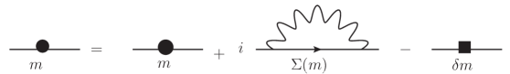
Figure 1: One-loop mass renormalization.

$$m=m+\Sigma(m)-\delta m^{(2)},$$ (8)

where $\delta m^{(2)}=\Sigma(m)$. This expression is illustrated in Fig. 1. The factor $i$ before the self-energy diagram in Fig. 1 is included in the standard diagrammatic definition of $\Sigma(p)$, see e.g., [29].

Next we turn to the matrix element of the EMT trace in Eq. (6) for the electron. The leading contribution to the matrix element of the term $(\beta(e_{0})/2e_{0})F_{0}^{2}$ in Eq. (7) is of order $\alpha^{2}$ and we ignore it. It is sufficient to calculate the one-loop matrix element

$$T=\langle\bm{0}|m_{0}(1+\gamma_{m})\bar{\psi}_{0}\psi_{0}|\bm{0}\rangle.$$ (9)

In the one-loop approximation

$$T=\langle\bm{0}|(1+\gamma_{m})m_{0}\bar{\psi}_{0}\psi_{0}|\bm{0}\rangle\approx\langle\bm{0}|(1+\gamma_{m})(m-\delta m^{(2)})\bar{\psi}_{0}\psi_{0}|\bm{0}\rangle$$ (10)

$$=m+m\delta Z_{2}-\delta m^{(2)}+m\gamma_{m}+\Gamma_{m}(m)$$

where $\Gamma_{m}(m)$ is the one-loop diagram for the scalar vertex $m\bar{\psi}\psi$, see Fig. 2.

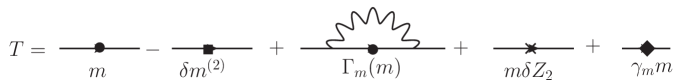
Figure 2: One-loop matrix element of the EMT trace.

All terms on the RHS in Eq. (10) and in Fig. 2, except $\Gamma_{m}(m)$, are known from the one-loop mass-shell renormalization scheme (see Eq. (27) and Eq. (28)) and only $\Gamma_{m}(m)$ requires calculation. After an easy one-loop calculation we obtain

$$\Gamma_{m}(m)=\frac{\alpha}{4\pi}m\left\{\frac{8}{\epsilon}-4\gamma+2\ln\frac{\lambda^{2}}{m^{2}}+4\ln\frac{\mu^{2}}{m^{2}}+2+4\ln(4\pi)\right\},$$ (11)

where $\lambda$ is the infrared photon mass and $\gamma$ is the Euler constant.

Next we use $\Gamma_{m}(m)$, the renormalization constants in Eq. (27) and Eq. (28), and $\gamma_{m}=3\alpha/2\pi$ to calculate the sum in Eq. (10)

$$T=m+m\delta Z_{2}-\delta m^{(2)}+m\gamma_{m}+\Gamma_{m}(m)=m.$$ (12)

Thus we confirmed that the matrix element $T$ of the anomalous EMT trace in the one-loop approximation is equal the physical electron mass, as it should be. Comparing Eq. (8) and Eq. (12) (and the respective Figs. 1 and 2) we see that

$$\Sigma(m)=\Gamma_{m}(m)+m\delta Z_{2}+\gamma_{m}m.$$ (13)

At this stage it is unclear why the different sets of diagrams in Fig. 1 and Fig. 2 produce coinciding results. To figure out a deeper reason why this happens we expand the unrenormalized electron self-energy $\Sigma(\not{p})$ in the Taylor series near the physical mass

$$\Sigma(\not{p})=\Sigma(\not{p}=m)+(\not{p}-m)\Sigma^{\prime}(\not{p}=m)+O((\not{p}-m)^{2})$$ (14)

$$=\delta m^{(2)}+(\not{p}-m)\delta Z_{2}+O((\not{p}-m)^{2}).$$

Differentiating with respect to $m$ we obtain at $\not{p}=m$

$$m\frac{d\Sigma(\not{p})}{dm}_{|\not{p}=m}=m\frac{d\Sigma(\not{p}=m)}{dm}-m\Sigma^{\prime}(\not{p}=m).$$ (15)

Notice that (see Fig. 3)

$$m\frac{d\Sigma(p)}{dm}=\Gamma_{m}(p),$$ (16)

Figure 3: Logarithmic mass derivative of $\Sigma(p)$.

which holds due to the identity

$$m\frac{d}{dm}\left(\frac{1}{\not{p}-m}\right)=\frac{1}{\not{p}-m}m\frac{1}{\not{p}-m}.$$ (17)

Then Eq. (15) can be written in the form

$$\Gamma_{m}(m)+m\delta Z_{2}=m\frac{d\Sigma(\not{p}=m)}{dm},$$ (18)

and Eq. (13) turns into ($\delta m^{(2)}=\Sigma(\not{p}=m)$)

$$\Sigma(m)=m\frac{d\Sigma(\not{p}=m)}{dm}+\gamma_{m}m\equiv m\frac{d(\delta m^{(2)})}{dm}+\gamma_{m}m.$$ (19)

We calculate the derivative on the RHS using the explicit expression for $\delta m^{(2)}$ in Eq. (27) and obtain (see Fig. 4)

$$m\frac{d(\delta m^{(2)})}{dm}=\delta m^{(2)}-\mu\frac{d\delta m^{(2)}}{d\mu}=\delta m^{(2)}-\gamma_{m}m,$$ (20)

where at the last step we used the definition of the electron mass anomalous dimension. Notice that this relationship holds due to a specific functional form of the mass counterterm $\delta m^{(2)}=mf(m/\mu)$ with some function $f$.

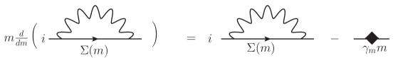
Figure 4: Logarithmic mass derivative of $\Sigma(m)$.

Thus we proved by direct calculation that Eq. (19) holds and the expressions in Eq. (8) and Eq. (12) (and the respective sets of diagrams in Fig. 1 and Fig. 2) coincide.

IV Conclusions

We have shown that the standard mass renormalization in Fig. 1 and the sum of the diagrams for the matrix element of the EMT trace in Fig. 2 coincide. This happens due to two important relationships. First, the one-loop diagram for a scalar vertex is equal to the logarithmic derivative of the self-energy diagram, see Eq. (16) and Fig. 3. Second, the mass renormalization counterterm (self-energy at $\not{p}=m$) is equal to its own logarithmic derivative plus the product of mass and its anomalous dimension, see Eq. (19) and Fig. 4.

The calculations above are made in the one-loop approximation, but we expect that they, including the functional relationship mentioned after Eq. (20), can be generalized to any number of loops. Really, connection between an arbitrary diagram and its logarithmic derivative with respect to the fermion mass, and the connection between such derivative and the fermion mass anomalous dimension do not depend on the number of loops, and these are the only essential steps in the derivation above.

Appendix A Standard one-loop electron mass renormalization

Some well known results are collected below. We use dimensional regularization and mass-shell renormalization. The QED Lagrangian in this scheme is

$${\cal L}_{0}=-\frac{1}{4}F_{0}^{2}+\bar{\psi}_{0}(i\not{\partial}-m_{0})\psi_{0}-e_{0}\bar{\psi}_{0}\not{A}_{0}\psi_{0}={\cal L}+\delta{\cal L},$$ (21)

where

$${\cal L}=-\frac{1}{4}F^{2}+\bar{\psi}(i\not{\partial}-m)\psi-\mu^{\frac{\epsilon}{2}}e\bar{\psi}\not{A}\psi,$$ (22)

$$\delta{\cal L}=-\frac{1}{4}\delta Z_{3}F^{2}+\bar{\psi}(i\delta Z_{2}\not{\partial}-\delta_{m})\psi-\mu^{\frac{\epsilon}{2}}e\delta Z_{1}\bar{\psi}\not{A}\psi,$$ (23)

$${\cal L}+\delta{\cal L}=-\frac{1}{4}Z_{3}F^{2}+iZ_{2}\bar{\psi}\not{\partial}\psi-mZ_{m}\bar{\psi}\psi-eZ_{1}\mu^{\frac{\epsilon}{2}}\bar{\psi}\not{A}\psi,$$ (24)

and

$$Z_{1}=1+\delta Z_{1},\quad Z_{2}=1+\delta Z_{2},\quad Z_{3}=1+\delta Z_{3},\quad mZ_{m}=m(1+\delta Z_{m})=m+\delta_{m}.$$ (25)

We define $\delta m=m-m_{0}=m-mZ_{m}Z_{2}^{-1}$. In the one-loop approximation $\delta m^{(2)}\approx-m\delta Z_{m}+m\delta Z_{2}=-\delta_{m}+m\delta Z_{2}$.

The renormalized one-loop self-energy $\Sigma_{r}(p)$ is

$$\begin{split}\Sigma_{r}(p)&=\frac{\alpha}{2\pi}\int_{0}^{1}dx\Biggl{\{}(2m-x\not{p})\left[\frac{2}{\epsilon}-\gamma+\ln(4\pi)+\ln\frac{\mu^{2}}{-x(1-x)p^{2}+x\lambda^{2}+(1-x)m^{2}}\right]\\ &-(m-x\not{p})\Biggr{\}}-(\not{p}\delta Z_{2}-\delta_{m})_{|\not{p}\to m}\\ &\approx\Sigma(m)+(\not{p}-m)\Sigma^{\prime}(\not{p}=m)-(\not{p}-m)\delta Z_{2}+(\delta_{m}-m\delta Z_{2})\\ &=\frac{3\alpha}{4\pi}m\left[\frac{2}{\epsilon}-\gamma+\ln(4\pi)+\ln\frac{\mu^{2}}{m^{2}}+\frac{4}{3}\right]\\ &-(\not{p}-m)\frac{\alpha}{4\pi}\left[\frac{2}{\epsilon}-\gamma+\ln(4\pi)+\ln\frac{\mu^{2}}{m^{2}}+2\ln\frac{\lambda^{2}}{m^{2}}+{4}\right]\\ &-(\not{p}-m)\delta Z_{2}+(\delta_{m}-m\delta Z_{2}),\end{split}$$ (26)

where $\Sigma(p)$ is the dimensionally regularized self-energy, $\mu$ is the auxiliary dimensional regularization mass, $\lambda$ is the IR photon mass and $\epsilon=4-d$.

The one-loop counterterms are

$$\delta m^{(2)}\equiv m\delta Z_{2}-\delta_{m}=\Sigma(m)=\frac{3\alpha}{4\pi}m\left[\frac{2}{\epsilon}-\gamma+\ln(4\pi)+\ln\frac{\mu^{2}}{m^{2}}+\frac{4}{3}\right],$$ (27)

$$\delta Z_{2}=\Sigma^{\prime}(\not{p}=m)=-\frac{\alpha}{4\pi}\left[\frac{2}{\epsilon}-\gamma+\ln(4\pi)+\ln\frac{\mu^{2}}{m^{2}}+2\ln\frac{\lambda^{2}}{m^{2}}+{4}\right].$$ (28)

- [1] I. Y. Kobzarev and L. B. Okun, “Gravitational interaction of fermions,” Zh. Eksp. Teor. Fiz. 43, 1904-1909 (1962).
- [2] H. Pagels, Energy-Momentum Structure Form Factors of Particles, Phys. Rev. 144, 1250-1260 (1966) doi:10.1103/PhysRev.144.1250.
- [3] X. D. Ji, Gauge-Invariant Decomposition of Nucleon Spin, Phys. Rev. Lett. 78, 610-613 (1997) doi:10.1103/PhysRevLett.78.610 [arXiv:hep-ph/9603249 [hep-ph]].
- [4] X. D. Ji, Deeply virtual Compton scattering, Phys. Rev. D 55, 7114-7125 (1997) doi:10.1103/PhysRevD.55.7114 [arXiv:hep-ph/9609381 [hep-ph]].
- [5] A. V. Radyushkin, Asymmetric gluon distributions and hard diffractive electroproduction, Phys. Lett. B 385, 333-342 (1996) doi:10.1016/0370-2693(96)00844-1 [arXiv:hep-ph/9605431 [hep-ph]].
- [6] J. C. Collins, L. Frankfurt and M. Strikman, “Factorization for hard exclusive electroproduction of mesons in QCD,” Phys. Rev. D 56, 2982-3006 (1997) doi:10.1103/PhysRevD.56.2982 [arXiv:hep-ph/9611433 [hep-ph]].
- [7] D. Kharzeev, H. Satz, A. Syamtomov and G. Zinovjev, J / psi photoproduction and the gluon structure of the nucleon, Eur. Phys. J. C 9, 459-462 (1999) doi:10.1007/s100529900047 [arXiv:hep-ph/9901375 [hep-ph]].
- [8] E. R. Berger, M. Diehl and B. Pire, “Time - like Compton scattering: Exclusive photoproduction of lepton pairs,” Eur. Phys. J. C 23, 675-689 (2002) doi:10.1007/s100520200917 [arXiv:hep-ph/0110062 [hep-ph]].
- [9] X. D. Ji, “A QCD analysis of the mass structure of the nucleon,” Phys. Rev. Lett. 74, 1071-1074 (1995) doi:10.1103/PhysRevLett.74.1071 [arXiv:hep-ph/9410274 [hep-ph]].
- [10] X. D. Ji, “Breakup of hadron masses and energy - momentum tensor of QCD,” Phys. Rev. D 52, 271-281 (1995) doi:10.1103/PhysRevD.52.271 [arXiv:hep-ph/9502213 [hep-ph]].
- [11] J. Hudson and P. Schweitzer, “D term and the structure of pointlike and composed spin-0 particles,” Phys. Rev. D 96, no.11, 114013 (2017) doi:10.1103/PhysRevD.96.114013 [arXiv:1712.05316 [hep-ph]].
- [12] M. V. Polyakov and P. Schweitzer, Forces inside hadrons: pressure, surface tension, mechanical radius, and all that, Int. J. Mod. Phys. A 33, no.26, 1830025 (2018) doi:10.1142/S0217751X18300259 [arXiv:1805.06596 [hep-ph]].
- [13] D. E. Kharzeev, “Mass radius of the proton,” Phys. Rev. D 104, no.5, 054015 (2021) doi:10.1103/PhysRevD.104.054015 [arXiv:2102.00110 [hep-ph]].
- [14] K. F. Liu, “Proton mass decomposition and hadron cosmological constant,” Phys. Rev. D 104, no.7, 076010 (2021) doi:10.1103/PhysRevD.104.076010 [arXiv:2103.15768 [hep-ph]].
- [15] C. Lorcé, A. Metz, B. Pasquini and S. Rodini, “Energy-momentum tensor in QCD: nucleon mass decomposition and mechanical equilibrium,” JHEP 11, 121 (2021) doi:10.1007/JHEP11(2021)121 [arXiv:2109.11785 [hep-ph]].
- [16] X. Ji, Y. Liu and I. Zahed, “Mass structure of hadrons and light-front sum rules in the Hooft model,” Phys. Rev. D 103, no.7, 074002 (2021) doi:10.1103/PhysRevD.103.074002 [arXiv:2010.06665 [hep-ph]].
- [17] K. A. Milton, “Quantum corrections to stress tensors and conformal invariance,” Phys. Rev. D 4, 3579-3593 (1971) doi:10.1103/PhysRevD.4.3579.
- [18] K. A. Milton, “Scale invariance and spectral forms for conformal stress tensors. (erratum),” Phys. Rev. D 7, 1120 (1973) [erratum: Phys. Rev. D 7, 3821 (1973)] doi:10.1103/PhysRevD.7.1120.
- [19] F. A. Berends and R. Gastmans, “Quantum Electrodynamical Corrections to Graviton-Matter Vertices,” Annals Phys. 98, 225 (1976) doi:10.1016/0003-4916(76)90245-1.
- [20] K. A. Milton, “Quantum Electrodynamic Corrections to the Gravitational Interaction of the electron,” Phys. Rev. D 15, 538 (1977) doi:10.1103/PhysRevD.15.538.
- [21] X. D. Ji and W. Lu, A Modern anatomy of electron mass, [arXiv:hep-ph/9802437 [hep-ph]].
- [22] S. Rodini, A. Metz and B. Pasquini, Mass sum rules of the electron in quantum electrodynamics, JHEP 09, 067 (2020) doi:10.1007/JHEP09(2020)067 [arXiv:2004.03704 [hep-ph]].
- [23] B. d. Sun, Z. h. Sun and J. Zhou, “Trace anomaly contribution to hydrogen atom mass,” Phys. Rev. D 104, no.5, 056008 (2021) doi:10.1103/PhysRevD.104.056008 [arXiv:2012.09443 [hep-ph]].
- [24] X. Ji, Y. Liu and A. Schäfer, Scale symmetry breaking, quantum anomalous energy and proton mass decomposition, Nucl. Phys. B 971, 115537 (2021) doi:10.1016/j.nuclphysb.2021.115537 [arXiv:2105.03974 [hep-ph]].
- [25] A. Metz, B. Pasquini and S. Rodini, “The gravitational form factor D(t) of the electron,” Phys. Lett. B 820, 136501 (2021) doi:10.1016/j.physletb.2021.136501 [arXiv:2104.04207 [hep-ph]].
- [26] X. Ji and Y. Liu, “Momentum-Current Gravitational Multipoles of Hadrons,” Phys. Rev. D 106, no.3, 034028 (2022) doi:10.1103/PhysRevD.106.034028 [arXiv:2110.14781 [hep-ph]].
- [27] X. Ji and Y. Liu, “Gravitational Tensor-Monopole Moment of Hydrogen Atom To Order ,” [arXiv:2208.05029 [hep-ph]].
- [28] A. Freese, A. Metz, B. Pasquini and S. Rodini, “The gravitational form factors of the electron in quantum electrodynamics,” [arXiv:2212.12197 [hep-ph]].
- [29] M. E. Peskin and D. V. Schroeder, “An Introduction to quantum field theory,” Addison-Wesley, 1995, ISBN 978-0-201-50397-5.
- [30] N. K. Nielsen, “The Energy Momentum Tensor in a Nonabelian Quark Gluon Theory,” Nucl. Phys. B 120, 212-220 (1977) doi:10.1016/0550-3213(77)90040-2.
- [31] S. L. Adler, J. C. Collins and A. Duncan, “Energy-Momentum-Tensor Trace Anomaly in Spin 1/2 Quantum Electrodynamics,” Phys. Rev. D 15, 1712 (1977) doi:10.1103/PhysRevD.15.1712.
- [32] J. C. Collins, A. Duncan and S. D. Joglekar, “Trace and Dilatation Anomalies in Gauge Theories,” Phys. Rev. D 16, 438-449 (1977) doi:10.1103/PhysRevD.16.438.
- [33] R. Tarrach, “The renormalization of FF,” Nucl. Phys. B 196, 45-61 (1982) doi:10.1016/0550-3213(82)90301-7.
- [34] Y. Hatta, A. Rajan and K. Tanaka, “Quark and gluon contributions to the QCD trace anomaly,” JHEP 12, 008 (2018) doi:10.1007/JHEP12(2018)008 [arXiv:1810.05116 [hep-ph]].
- [35] K. Tanaka, “Three-loop formula for quark and gluon contributions to the QCD trace anomaly,” JHEP 01, 120 (2019) doi:10.1007/JHEP01(2019)120 [arXiv:1811.07879 [hep-ph]].
- [36] A. Metz, B. Pasquini and S. Rodini, “Revisiting the proton mass decomposition,” Phys. Rev. D 102, 114042 (2020) doi:10.1103/PhysRevD.102.114042 [arXiv:2006.11171 [hep-ph]].
- [37] T. Ahmed, L. Chen and M. Czakon, “A note on quark and gluon energy-momentum tensors,” [arXiv:2208.01441 [hep-ph]].
- [38] K. Tanaka, “Twist-four gravitational form factor at NNLO QCD from trace anomaly constraints,” [arXiv:2212.09417 [hep-ph]].