22email: mike.giles@maths.ox.ac.uk
MLMC techniques for discontinuous functions
Abstract
The Multilevel Monte Carlo (MLMC) approach usually works well when estimating the expected value of a quantity which is a Lipschitz function of intermediate quantities, but if it is a discontinuous function it can lead to a much slower decay in the variance of the MLMC correction. This article reviews the literature on techniques which can be used to overcome this challenge in a variety of different contexts, and discusses recent developments using either a branching diffusion or adaptive sampling.
1 Introduction
The Multilevel Monte Carlo (MLMC) method is based on the telescoping sum
where represents an approximation to an output quantity of interest on level , with the weak error and MLMC variance , both decreasing as the level increases, but with the corresponding computational cost per sample increasing.
If has expected value , with , with variance and cost , then for a given target RMS error , the number of levels and the number of independent samples on each level can be optimised Gi_giles08 ; Gi_giles15 to give an overall cost which is approximately equal to
If as , then the cost is dominated by the first term from level , and the cost is approximately , so proportional to .
If as , then the contributions to the cost are spread almost equally across all levels and the cost is approximately , proportional to if decays exponentially with .
Even worse, if as , then the cost is dominated by the contribution from the finest level and so is approximately which is if , and .
In most MLMC applications, is a smooth, or at least Lipschitz, function of some intermediate solution quantities, such as the solution of an SDE, a PDE with stochastic coefficients or initial/boundary data, or an estimate of an inner conditional expectation. Under these circumstances we usually have and so the MLMC complexity is or .
This article is concerned with the small but important class of applications where is a discontinuous function of the intermediate quantities, and because of this the MLMC variance can decay much more slowly, leading to the complexity falling into the third category of being .
The good news is that there has been considerable research within the MLMC community 111See https://people.maths.ox.ac.uk/gilesm/mlmc_community.html to address this challenge. This article surveys the variety of methods which have been developed in the hope that this can aid researchers meeting similar challenges in future applications.
To illustrate things, we begin by detailing two specific application challenges which have motivated much of this research. We then discuss the many approaches which have been developed, several of which have borrowed ideas from the literature on computing sensitivities (the “greeks” in mathematical finance literature) of the form using the pathwise sensitivity approach Gi_glasserman04 (also known as Infinitesimal Perturbation Analysis, IPA for short Gi_ecuyer90 ) or Likelihood Ratio Method Gi_ecuyer95 , or from methods for improving integrand smoothness to improve the rate of convergence for QMC integration Gi_acn13 ; Gi_bst18 .
1.1 Challenge 1: nested expectation
Suppose is a scalar function and we want to estimate the nested expectation , where the outer expectation is with respect to a random variable and we will assume that the inner conditional expectation has a bounded density near zero.
A very simple MLMC treatment 222Note that if is smooth, or at least Lipschitz, then it is better to use an “antithetic” estimator Gi_bhr15 ; Gi_giles15 ; Gi_giles18 ; Gi_gg19 , but this does not give a better order of convergence when is discontinuous. uses inner samples on level , so estimators on level and the higher levels are simply
where and represent independent averages of and independent samples of , all conditional on the same value of Gi_giles15 ; Gi_giles18 .
If is finite, and is Lipschitz with constant , then
and hence for . If is uniformly bounded it follows that . If the cost of each conditional sample of is then and hence the complexity is .
Unfortunately, the situation is significantly poorer when is the Heaviside step function defined by if , and if . This occurs in many applications because so it corresponds to the probability of a conditional expectation exceeding some threshold , which is a very important quantity in risk calculations.
If and has a bounded density near zero then there is an probability that , which is the circumstance under which there is an probability that due to being positive and being negative, or vice versa. Hence and the complexity is approximately Gi_gh19 .
This challenge is the primary motivation for Section 7, and also arises in the context of Section 3.
1.2 Challenge 2: discontinuous payoff function
In the case of a scalar SDE
| (1) |
with an output quantity of interest , the standard estimator is
where the same Brownian motion is used to calculate both and , but with different uniform timesteps and .
If is Lipschitz with constant , then
where is the level numerical approximation to . Hence, based on standard strong convergence results Gi_kp92 we have for an Euler-Maruyama discretisation of the SDE, and for the first order Milstein discretisation. The cost is in both cases, giving MLMC complexities of and , respectively,
In mathematical finance, a digital call option payoff is or , depending on whether is below or above the strike , so the payoff function can be written as . The MLMC problem is that a small difference between the coarse and fine paths can give a payoff difference of if the two paths straddle the strike, i.e. are on different sides of the strike.
When using the Euler-Maruyama approximation of the SDE, . Speaking loosely (see Gi_avikainen09 ; Gi_ghm09 for the rigorous analysis) an fraction of fine/coarse pairs straddle the strike, so and hence the complexity is .
Similarly, using the Milstein approximation gives so . This is clearly better, and gives a complexity which is , but there is still the problem that most MLMC samples are zero on the finer levels, so the kurtosis is which causes problems in practice in estimating accurately to determine the number of samples to use on level . In addition, there is the difficulty that the Milstein discretisation of multi-dimensional SDEs often requires the simulation of Lévy areas, though this problem can be addressed through the use of an antithetic estimator Gi_gs14 .
This challenge is the primary motivation for Sections 2, 4, 5 and 6, also also arises in Sections 3 and 7.
2 Explicit smoothing
The pathwise sensitivity analysis (or IPA) approach to compute the parameter sensitivities known as Greeks in mathematical finance Gi_glasserman04 requires that the payoff function is continuous and piecewise smooth. This is clearly a problem with digital options, and one standard approach in this case is to smooth the payoff function by replacing the Heaviside step function with a smoothed approximation , with as and as , so the discontinuity is smoothed over a width of .
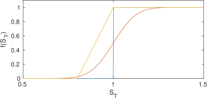
For financial reasons, the preference is often to use a one-sided smoothing, such as the piecewise linear approximation shown in yellow in Figure 1. This one-sided approximation introduces a weak error, or bias, which is . If it is used for MLMC, then for the fraction of the paths which end up in the ramp region, and therefore . Hence the optimal choice of involves a tradeoff between bias and variance.
The bias can be reduced by making the smoothing anti-symmetric about so that , for example by choosing as illustrated in orange in Figure 1. If has the smooth probability density then the weak error is
and a Taylor series expansion of results in the asymptotic error expansion
where
If then , and
If is monotonic, then , but by considering non-monotonic functions such as it is possible to set making the weak error . Hence, to achieve accuracy overall we need , and then on the coarsest levels so the overall complexity is approximately in the best cases where the overall cost is dominated by the cost on the coarsest levels.
Giles, Nagapetyan & Ritter Gi_gnr15 used explicit smoothing for estimating cumulative distribution functions (CDFs). For a scalar random variable , to estimate , the approach they adopted was to use MLMC to estimate for a set of spline points and then interpolate these values with a cubic spline. Overall, their method balanced three weak errors, the SDE discretisation error on the finest level, the smoothing error due to , and the cubic spline interpolation error, in addition to the MLMC sampling error.
3 Integration/differentiation and Malliavin calculus
Krumscheid & Nobile Gi_kn18 used a slightly different approach for estimating CDFs, particularly in the context of risk estimation. Starting from the identity
they used MLMC to estimate for a set of spline points , interpolated these with a cubic spline, and and then differentiated the spline to obtain an approximation to the CDF . This avoids the extra weak error due to smoothing the Heaviside function, but differentiating the cubic spline amplifies the noise in the spline data.
On a similar note, Altmayer & Neuenkirch Gi_an15 used Malliavin calculus integration by parts to treat discontinuous payoffs based on solutions of the Heston stochastic volatility SDE. They observed that asymptotically this improves the MLMC variance on the finer levels, but it increases the variance on coarse levels. To address this, they split the payoff into a smooth part which they treated with the standard MLMC approach, and a compact-support discontinuous part for which they used the Malliavin MLMC.
Malliavin calculus was originally developed for computing sensitivities, so this is another example of the literature on sensitivity calculations being exploited to develop improved MLMC algorithms.
4 Conditional expectation
When using the first order Milstein discretisation for an SDE, one way to improve the MLMC variance for digital options is to switch to the Euler-Maruyama approximation for the final timestep, and then take the conditional expectation with respect to the final fine path Brownian increment Gi_giles08b ; Gi_gdr19 .
For the fine path approximation of the scalar SDE (1) with timesteps of size , the path value at the final time is given by
and therefore the conditional expected value for the digital call option is
Similarly, for the coarse path with coarse timestep , the Brownian increment for the final coarse timestep is the sum of the last two Brownian increments for the fine path, , and therefore
from which we obtain
With , numerical analysis Gi_gdr19 proves that so the MLMC complexity is . Heuristically, this is because there is an probability of paths being within of the strike , and for these
so . In addition, the kurtosis is improved to . Unfortunately, this approach does not help when the Euler-Maruyama discretisation is used for the entire path since and so
The use of this kind of conditional expectation is a standard technique for smoothing the payoff to enable IPA/pathwise sensitivity calculations Gi_glasserman04 . Another example is a down-and-out barrier option, where the option is knocked out if the path drops below a certain value. In this case the payoff can be smoothed by computing the probability of this happening, conditional on the computed path approximations at discrete timesteps Gi_glasserman04 . Again, this works well for MLMC when using the first order Milstein discretisation Gi_giles08b ; Gi_gdr19 , but it does not help with the Euler-Maruyama discretisation.
A different kind of conditional expectation smoothing was introduced by Achtsis, Cools & Nuyens Gi_acn13 and Bayer, Siebenmorgen & Tempone Gi_bst18 to improve the convergence of QMC computations, and then used by Bayer, Ben Hammouda & Tempone Gi_bht20 to improve the MLMC variance for digital options.
In its simplest form, they split the random inputs for the numerical simulation into a scalar and the remainder , and express the desired MLMC level expectation as
and observe that in many financial applications it is possible to perform this split in a way such that the conditional expectations are smooth functions of , and can be evaluated analytically or very accurately by 1D numerical quadrature when there is just a single discontinuity with respect to changes in .
For a scalar SDE, could be the terminal value of the driving Brownian motion, in which case would represent the other Normal random variables required for a Brownian Bridge construction of the Brownian increments.
5 Change of measure
Another approach to treating digital options using the Milstein discretisation is to use a change of measure Gi_burgos14 ; Gi_giles15 , which has connections to the Likelihood Ratio Method (LRM) that is used for sensitivity analysis Gi_ecuyer95 .
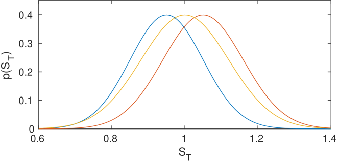
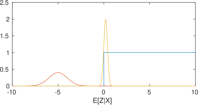
For both the fine and coarse paths, we have conditional Gaussian distributions for , with slightly different means and variances, as illustrated in Figure 2. We can therefore perform a change of measure to the same Gaussian distribution with mean and variance , also illustrated in Figure 2, and then pick the same sample for both paths from this common Gaussian distribution.
The resulting MLMC estimator is
where are the respective Radon-Nikodym derivatives for the fine and coarse paths. For the scalar SDE (1), is
and is defined similarly. It can be shown that the difference is approximately , which implies that . To improve the variance we note that the conditional expected value of Radon-Nikodym derivatives is always 1, i.e. , and therefore we can change the definition of to
without changing its expected value. This estimator is now non-zero only when and are on opposite sides of the strike , which occurs for an fraction of coarse/fine paths. Hence the new MLMC variance is approximately , as with the use of the analytic conditional expectation.
The benefit of this approach is that it works well in multiple dimensions when it is often not possible to evaluate the analytic conditional expectation Gi_burgos14 ; Gi_giles15 . However, again it does not help with the full path Euler-Maruyama discretisation because that gives .
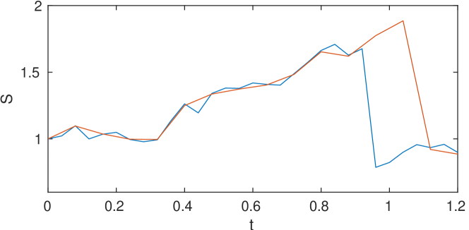
An earlier use of a change of measure in an MLMC computation was by Xia Gi_xia14 ; Gi_xg12 for a Merton-style jump-diffusion SDE with a path-dependent jump rate . The challenge in this application, as illustrated in Figure 3, is that the coarse and fine paths will jump at different times, and one might jump just before the final time , and the other just after, leading to a large difference in the computed value of . The path-dependent jump rate was treated by using the thinning technique of Glasserman & Merener Gi_gm04 , over-sampling possible jump times using a uniform rate and then using an acceptance/rejection step to select the real jump times. Xia modified this with a change of measure to ensure the same acceptance/rejection decision for both the fine and coarse paths so that they both jump at the same time. This leads to an estimator of the form
When combined with a first order Milstein discretisation of the SDE between the jump times, this gives for Lipschitz payoff functions such as a standard put or call option Gi_xia14 ; Gi_xg12 .
6 Splitting
Returning to the challenge of digital options arising from the solution of an SDE, a third approach is to use path-splitting to generate an unbiased estimate of the conditional expectation introduced in Section 4 Gi_giles15 .
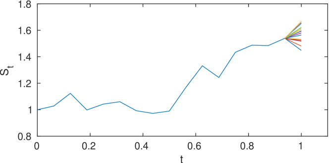
This is a variant of the general splitting technique Gi_ag07 . As illustrated in Figure 4, it involves performing a standard fine path simulation up until one timestep before the final time , and then performing multiple independent simulations of the final timestep, averaging the payoff for each of these to get an approximation of the conditional expectation. The same is done for the coarse path except that each of the splits uses the same that was used for the second to last fine path timestep.
Since the computational cost of the path up to the splitting time is , it means that up to splits can be used without increasing the path cost significantly. If splits are used, then the standard splitting variance analysis gives
As discussed previously , and similarly it can be argued that . Therefore choosing to lie between and ensures the benefits of the splitting are obtained without significantly increasing the computational cost per sample.
As an additional bonus, one can use the more accurate Milstein discretisation for the final timestep, instead of switching to the Euler-Maruyama discretisation. Burgos Gi_burgos14 ; Gi_bg12 gives more details of the analysis, and also used the same approach for pathwise sensitivity analysis for a variety of financial options.
Giles & Bernal Gi_gb18 also used splitting for Feynman-Kac functionals arising for stopped diffusions, SDE simulations which terminate when the solution path leaves a prescribed domain. The issue here is that when a fine path exits, there is an probability that the corresponding coarse path does not leave until much later. This is addressed by estimating a conditional expectation by splitting the coarse path into independent sub-simulations which continue until each of them leaves the domain. is improved from to approximately without a significant increase in the cost per sample, and finally the MLMC complexity achieved is .
None of the three methods introduced so far (conditional expectation, change of measure, splitting) helps when using the Euler-Maruyama discretisation. For this, a new method has recently been developed by Giles & Haji-Ali Gi_gh22b .
It again uses splitting, but inspired by the simulation of branching diffusions, it considers splits at multiple deterministic times, as illustrated in Figure 5 which shows the logical structure of a set of split paths. Here we are considering a simulation on the unit time interval. A single pair of fine/coarse paths is calculated up to time , with the number of fine timesteps being . This simulation is then split into two separate independent simulations up to time , with the two simulations between them accounting for an additional fine timesteps. There are further splits at , then at , and so on, with the final split when there is just one coarse timestep left.
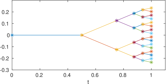
The total number of fine timesteps simulated is so the computational cost is only slightly increased compared to the original method with a single pair of fine/coarse paths. is defined to be the average of the values for each of the final paths, and it can be proved that its variance is , the same asymptotic order of convergence as for Lipschitz payoff functions Gi_gh22b . The kurtosis is also improved, so this technique fully addresses the challenge of using MLMC with the Euler-Maruyama discretisation to estimate digital option values.
7 Adaptive sampling
We return now to the challenge of estimating the nested expectation and we note that we only need an accurate estimate of the inner conditional expectation when it is near zero. This observation is the basis for the development of adaptive sampling by Broadie, Du & Moallemi Gi_bdm11 within a standard Monte Carlo procedure. This was then extended to adaptive sampling combined with MLMC by Giles & Haji-Ali Gi_gh19 by defining the number of inner samples on level to be
-
•
inner samples when
This is the smallest number of samples used on level . is the standard deviation of the Monte Carlo estimate for , so the inequality means that this number of samples is sufficient to be very sure that the estimate has the correct sign.
-
•
inner samples when
This is the maximum number of samples used on level . In this case, the estimate of may have the incorrect sign, but this will only happen when which occurs with probability . Likewise, the total cost of the higher number of samples in this region is , so it does not significantly increase the overall average cost.
-
•
for intermediate values
In this region the number of samples is chosen to be very sure that the estimate of has the correct sign, and at the same time the total cost is .
Overall, this adaptive sampling approach leads to , and hence a complexity of roughly Gi_gh19 . However, the kurtosis is since only an fraction of the outer samples give non-zero values for .
Haji-Ali, Spence & Teckentrup Gi_hst22 have further extended this to estimate quantities of the form
where is a -dimensional random variable which cannot be sampled directly. In their paper they consider in particular the two challenges in this article. In the context of the digital option with the Euler-Maruyama discretisation on the unit time interval, the adaptive sampling varies the timestep used on level so that
-
•
when is large compared to the strong error in the path approximation
-
•
when is of the same order as the strong error
-
•
for intermediate values
A Brownian bridge construction is used when the timestep needs to be refined as part of the adaptation procedure from its initial value . The adaptation again leads to , and hence a complexity of roughly , but there is again a high kurtosis Gi_hst22 .
In earlier research, Elfverson, Hellman & Malqvist Gi_ehm16 considered estimation of where cannot be sampled exactly but there is a sequence of approximations of increasing accuracy and increasing cost. Motivated by PDE applications with a well-behaved truncation error so that there are uniform geometric bounds on , level in their method uses
and achieves similarly good MLMC benefits. This idea is essentially the same as in the work of Haji-Ali et al but requiring a uniform bound on is significantly more restrictive than the bounds on for some required by Haji-Ali et al.
A final comment is that the analysis of Haji-Ali, Spence & Teckentrup can be generalised to a product of an indicator function and a Lipschitz function, , and so can handle barrier options. Furthermore, Haji-Ali & Spence have extended the adaptive sampling methodology to an extremely challenging triply-nested expectation which arises in mathematical finance Gi_ghs23 . By incorporating the randomised MLMC treatment of Rhee & Glynn Gi_rg15 to handle the time discretisation of the underlying SDEs as well as the sampling for the inner conditional expectations, they achieve an overall complexity of approximately which is very impressive for such a difficult application.
8 Conclusions
It is worth repeating that in most MLMC applications the output quantity of interest is a Lipschitz function of the intermediate simulation quantities, so good strong convergence for the intermediate quantities leads automatically to a good rate of convergence of the MLMC variance .
For those applications in which the function is discontinuous, this article shows there is an extensive literature with a variety of different approaches to improve the MLMC variance and try to recover the optimal complexity. It is notable that many of these methods have adapted ideas from Monte Carlo sensitivity analysis which also has problems with discontinuous functionals. It is hoped that this survey will assist future researchers facing similar challenges in other new application areas.
Acknowledgements.
This paper is based on research with many students, postdocs and other collaborators and I am grateful to all of them. Funding for the research has been provided by the UK Engineering and Physical Sciences Research Council through grants EP/E031455/1, EP/H05183X/1 and EP/P020720/2 as well as the Hong Kong Innovation and Technology Commission (InnoHK Project CIMDA). The paper was written while visiting the Oden Institute for Computational Engineering & Sciences at UT Austin, and I thank my hosts for their warm hospitality.References
- (1) N. Achtsis, R. Cools, and D. Nuyens. Conditional sampling for barrier option pricing under the LT method. SIAM Journal on Financial Mathematics, 4:327–352 (2013)
- (2) M. Altmayer and A. Neuenkirch. Multilevel Monte Carlo quadrature of discontinuous payoffs in the generalized Heston model using Malliavin integration by parts. SIAM Journal on Financial Mathematics, 6(1):22–52 (2015)
- (3) S. Asmussen and P.W. Glynn. Stochastic Simulation. Springer, New York (2007)
- (4) R. Avikainen. On irregular functionals of SDEs and the Euler scheme. Finance and Stochastics, 13(3):381–401 (2009)
- (5) C. Bayer, C. Ben Hammouda, and R. Tempone. Multilevel Monte Carlo combined with numerical smoothing for robust and efficient option pricing and density estimation. arXiv preprint: 2003.05708 (2020)
- (6) C. Bayer, M. Siebenmorgen, and R. Tempone. Smoothing the payoff for efficient computation of basket option prices. Quantitative Finance, 18(3):491–505 (2018)
- (7) M. Broadie, Y. Du, and C.C. Moallemi. Efficient risk estimation via nested sequential simulation. Management Science, 57(6):1172–1194 (2011)
- (8) K. Bujok, B. Hambly, and C. Reisinger. Multilevel simulation of functionals of Bernoulli random variables with application to basket credit derivatives. Methodology and Computing in Applied Probability, 17(3):579–604 (2015)
-
(9)
S. Burgos.
The computation of Greeks with multilevel Monte Carlo.
DPhil thesis, University of Oxford (2014)
https://ora.ox.ac.uk/objects/uuid:6453a93b-9daf-4bfe-8c77-9cd6802f77dd - (10) S. Burgos and M.B. Giles. Computing Greeks using multilevel path simulation. In L. Plaskota and H. Woźniakowski, editors, Monte Carlo and Quasi-Monte Carlo Methods 2010, pages 281–296. Springer (2012)
- (11) D. Elfverson, F. Hellman, and A. Målqvist. A multilevel Monte Carlo method for computing failure probabilities. SIAM/ASA Journal on Uncertainty Quantification, 4(1):312–330 (2016)
- (12) M.B. Giles. Improved multilevel Monte Carlo convergence using the Milstein scheme. In A. Keller, S. Heinrich, and H. Niederreiter, editors, Monte Carlo and Quasi-Monte Carlo Methods 2006, pages 343–358. Springer (2008)
- (13) M.B. Giles. Multilevel Monte Carlo path simulation. Operations Research, 56(3):607–617 (2008)
- (14) M.B. Giles. Multilevel Monte Carlo methods. Acta Numerica, 24:259–328 (2015)
- (15) M.B. Giles. MLMC for nested expectations. In Contemporary Computational Mathematics - A Celebration of the 80th Birthday of Ian Sloan. Springer (2018)
- (16) M.B. Giles and F. Bernal. Multilevel estimation of expected exit times and other functionals of stopped diffusions. SIAM/ASA Journal on Uncertainty Quantification, 6(4):1454–1474 (2018)
- (17) M.B. Giles, K. Debrabant, and A. Rößler. Analysis of multilevel Monte Carlo path simulation using the Milstein discretisation. Discrete and Continuous Dynamical Systems - series B, 24(8):3881–3903 (2019)
- (18) M.B. Giles and T. Goda. Decision-making under uncertainty: using MLMC for efficient estimation of EVPPI. Statistics and Computing, 29(4):739–751 (2019)
- (19) M.B. Giles and A.-L. Haji-Ali. Multilevel nested simulation for efficient risk estimation. SIAM/ASA Journal on Uncertainty Quantification, 7(2):497–525 (2019)
- (20) M.B. Giles and A.-L. Haji-Ali. Multilevel path branching for digital options. arXiv pre-print: 2209.03017 (2022)
- (21) M.B. Giles, A.-L. Haji-Ali and J. Spence. Efficient risk estimation for the credit valuation adjustment. arXiv pre-print: 2301.05886 (2023)
- (22) M.B. Giles, D.J. Higham, and X. Mao. Analysing multilevel Monte Carlo for options with non-globally Lipschitz payoff. Finance and Stochastics, 13(3):403–413 (2009)
- (23) M.B. Giles, T. Nagapetyan, and K. Ritter. Multilevel Monte Carlo approximation of distribution functions and densities. SIAM/ASA Journal on Uncertainty Quantification, 3(1):267–295 (2015)
- (24) M.B. Giles and L. Szpruch. Antithetic multilevel Monte Carlo estimation for multi-dimensional SDEs without Lévy area simulation. Annals of Applied Probability, 24(4):1585–1620 (2014)
- (25) P. Glasserman. Monte Carlo Methods in Financial Engineering. Springer, New York (2004)
- (26) P. Glasserman and N. Merener. Convergence of a discretization scheme for jump-diffusion processes with state-dependent intensities. Proc. Royal Soc. London A, 460:111–127 (2004)
- (27) A.-L. Haji-Ali, J. Spence, and A. Teckentrup. Adaptive multilevel Monte Carlo for probabilities. SIAM Journal on Numerical Analysis, 60(4):2125–2149 (2022)
- (28) P.E. Kloeden and E. Platen. Numerical Solution of Stochastic Differential Equations. Springer, Berlin (1992)
- (29) S. Krumscheid and F. Nobile. Multilevel Monte Carlo approximation of functions. SIAM/ASA Journal on Uncertainty Quantification, 6(3):1256–1293 (2018)
- (30) P. L’Ecuyer. A unified view of the IPA, SF and LR gradient estimation techniques. Management Science, 36(11):1364–1383 (1990)
- (31) P. L’Ecuyer. On the interchange of derivative and expectation for likelihood ratio derivative estimators. Management Science, 41(4):738–748 (1995)
- (32) C.-H. Rhee and P.W. Glynn. Unbiased estimation with square root convergence for SDE models. Operations Research, 63(5):1026–1043 (2015)
- (33) Y. Xia. Multilevel Monte Carlo for jump processes. DPhil thesis, University of Oxford (2014) https://ora.ox.ac.uk/objects/uuid:7bc8e98a-0216-4551-a1f3-1b318e514ee8/
- (34) Y. Xia and M.B. Giles. Multilevel path simulation for jump-diffusion SDEs. In L. Plaskota and H. Woźniakowski, editors, Monte Carlo and Quasi-Monte Carlo Methods 2010, pages 695–708. Springer (2012)