Model-Agnostic Hierarchical Attention for 3D Object Detection

Abstract

Transformers as versatile network architectures have recently seen great success in 3D point cloud object detection. However, the lack of hierarchy in a plain transformer makes it difficult to learn features at different scales and restrains its ability to extract localized features. Such limitation makes them have imbalanced performance on objects of different sizes, with inferior performance on smaller ones. In this work, we propose two novel attention mechanisms as modularized hierarchical designs for transformer-based 3D detectors. To enable feature learning at different scales, we propose Simple Multi-Scale Attention that builds multi-scale tokens from a single-scale input feature. For localized feature aggregation, we propose Size-Adaptive Local Attention with adaptive attention ranges for every bounding box proposal. Both of our attention modules are model-agnostic network layers that can be plugged into existing point cloud transformers for end-to-end training. We evaluate our method on two widely used indoor 3D point cloud object detection benchmarks. By plugging our proposed modules into the state-of-the-art transformer-based 3D detector, we improve the previous best results on both benchmarks, with the largest improvement margin on small objects.

1 Introduction

3D point cloud data provides accurate geometric and spatial information, which are important to computer vision applications such as autonomous driving and augmented reality. Different from image data, which has a grid-like structure, point clouds consist of unordered irregular points. Due to such unique properties of point clouds, previous works have proposed various deep network architectures for point cloud understanding [24, 37, 34, 7, 8, 23, 25, 22, 48, 50]. With the success of transformers in natural language processing [40, 4, 26] and 2D vision [5, 39, 14], attention-based architectures for point clouds [55, 20, 53, 52, 49, 46, 38] are explored in recent works and have seen great success in 3D point cloud object detection [45, 19, 16, 32]. Several properties of transformers make them ideal for learning on raw point clouds. For example, their permutation-invariant property is necessary for modeling unordered sets like point clouds, and their attention mechanism can model long-range relationships that help capture the global context for point cloud learning.

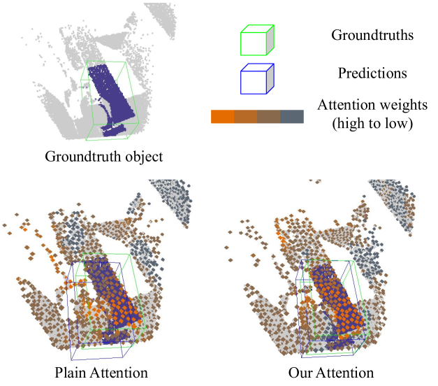
Figure 1: Visualization of the attention weights. With our hierarchical attentions, the object center has higher attention weights with points that belong to the object, and the predicted bounding box is better aligned with the groundtruth. Our multi-scale attention extracts feature at different scales, which helps distinguish object boundaries. Our size-adaptive local attention aggregates features at the object level and helps refine the bounding box proposals.

Despite the advantages of transformers for point clouds, we find the state-of-the-art transformer detector to have imbalanced performance across different object sizes, with the lowest average precision on small objects (see Section 4.3). We speculate the inferior performance on small objects can be due to two factors. Firstly, to make the computation feasible, transformer detectors use point cloud features consisting of a small set of points compared to the original point cloud. The extensively downsampled point cloud loses geometric details, which has a larger impact on small objects. Secondly, plain transformers (e.g., Transformer [40], ViT [5]) extract features at the global scale throughout the network, which does not support explicit localized feature learning.

Motivated by the above observations, we expect existing point cloud transformers to benefit from a hierarchical feature learning strategy, which allows multi-scale feature learning and supports localized feature aggregation. Nonetheless, considering the computation intensity of point cloud transformers, it is inefficient to use higher-resolution (i.e., higher point density) point cloud features throughout the network. Furthermore, due to the irregularity of point clouds, it is non-trivial to integrate hierarchical design and multi-scale features into transformers for point cloud object detection.

Our approach. In this work, we aim to improve transformer-based 3D object detectors with modularized hierarchical designs. We propose two attention modules for multi-scale feature learning and size-adaptive local feature aggregation. Our attention modules are model-agnostic and can be plugged into existing point cloud transformers for end-to-end training.

We first propose Simple Multi-Scale Attention (MS-A). It builds higher resolution point features from the single-scale input feature with a learnable upsampling strategy and use both features in the attention function. To reduce computation and parameter overhead, we transform the multi-scale features into multi-scale tokens and perform multi-scale token aggregation [30] within a multi-head attention module. The second module is Size-Adaptive Local Attention (Local-A), which learns localized object-level features for each object candidate. It assigns larger attention regions to object candidates with larger bounding box proposals. The local attention regions are defined by their corresponding intermediate bounding box proposals.

We evaluate our method on two widely used indoor 3D object detection benchmarks: ScanNetV2 [3] and SUN RGB-D [36]. We plug our attention modules into the state-of-the-art transformer-based 3D detector and perform end-to-end training. Our method improves the previous best result by over 1% in mAP@0.25 and over 2% in mAP@0.50 on ScanNetV2. Furthermore, our size-aware evaluation shows we have the most performance gain among small objects with a 2.5% increase in mAP_S. We summarize our main contributions as follows:

• We propose Simple Multi-Scale Attention (MS-A) to enable multi-scale feature learning on single-scale features.

• We present Size-Adaptive Local Attention (Local-A) for local feature aggregation within bounding box proposals.

• We conduct experiments on two widely used indoor 3D detection benchmarks and surpass the previous best results on both benchmarks.

2 Related Work

Network architectures for point cloud learning.

Existing network architectures for point cloud learning can be roughly divided into two categories based on their point cloud representation: grid-based and point-based, yet in between, there also exist hybrid architectures that operate on both representations [57, 9, 33, 51, 53]. Grid-based methods project the irregular point clouds into grid-like structures, such as 3D voxels. With the grid-like structure, existing works have proposed a variety of 3D-convolution-based architectures [18, 31, 42, 7]. Point-based methods, on the other hand, directly learn features from the raw point cloud. Within this category, graph-based method [35, 8, 44, 47, 56] use a graph to model the relationships among the points. Another line of work models a point cloud as a set of points, and extracts features through set abstraction [23, 25, 17, 41]. Recent works explore transformer architecture for point-based learning [55, 16, 19, 20, 53], where each point is fed into the transformer as a token and the attention mechanism learns point features at a global scale. While previous methods improve point cloud learning by developing new backbones and modifying the overall network architecture, our work focuses on the attention mechanism of the point cloud transformer. Instead of proposing new architectures for point cloud learning, we aim to provide a model-agnostic solution.

Point cloud object detection.

One major challenge in point cloud object detection is extracting object features. In 2D object detection, a common practice for extracting object features is to use a region proposal network (RPN) [29] to generate dense bounding box proposals (i.e., object candidate) in a top-down manner and then extract features for each object candidate. However, in 3D vision, generating dense 3D bounding box proposals for point cloud data is inefficient due to the irregularity and sparsity of point clouds. Previous work [2, 57] addresses this issue by projecting point clouds into 2D bird’s-eye views or voxels and then applying RPN. However, such projection operations can result in the loss of geometric information or introduce quantization errors. Another line of work seeks to generate 3D proposals in a bottom-up manner (i.e., point-based)  [34, 21, 16, 19]. VoteNet [21] samples a set of points from a point cloud as the initial object candidates and then assigns points to each object candidate through voting. Object features of each candidate are learned by aggregating features within its corresponding vote cluster (i.e., group). Instead of voting and grouping, follow-up works [16, 19] propose to use a transformer to automatically model the relationship between the object candidates and the point cloud. Although point-based methods do not have quantization errors caused by voxelization, to make the computation feasible, a point cloud needs to be extensively downsampled at the beginning of the model. Such downsampling also causes a loss of geometric information, while it is important for object detection to have fine-grained features to make accurate predictions. Our work is based on point-based transformer detectors. We address the downsampling issue by building higher-resolution features without increasing the computation budget.

Hierarchical designs for 2D and 3D vision transformers.

Extensive work has been done to adapt transformers for vision recognition. One direction is to borrow the hierarchical design and inductive biases from convolutional neural networks (ConvNet) [10]. In the 2D vision, one line of ConvNet-based hierarchical design [6, 11, 43] produces multi-scale feature maps for 2D images by progressively decreasing the resolution and expanding feature channels. Swin Transformer [15] adopts the idea of weight-sharing of ConvNet and proposes efficient self-attention with shifted windows. Shunted self-attention [30] attends to features at different scales through multi-scale token aggregation. In the 3D vision, hierarchical designs for point cloud transformers are explored in previous works, where self-attentions are applied to local regions (specified by $k$ nearest neighbors [55] or a given radius [20]), and downsampling operations are performed after every encoding stage following the hierarchical design of PointNet++ [25]. Patchformer [53] proposes a multi-scale attention block that performs extracts features at multiple granularities, but it requires voxelization on the point cloud. Different from previous works, we pack our hierarchical design into model-agnostic attention modules that can be plugged into any existing architecture and enable both multi-scale and localized feature learning.

3 Method

In this section, we first discuss the background, including a brief introduction to the task of point cloud object detection, an overview of point-based 3D detection methods, and the attention mechanism. Next, we dive into the detailed designs of our proposed attention modules.

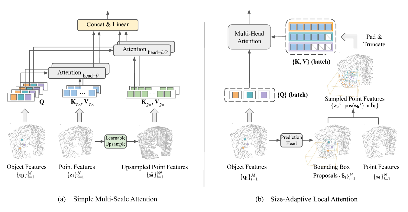
Figure 2: An illustration of our hierarchical attention modules. (a). Simple Multi-Scale Attention (MS-A) learns features at different scales within the multi-head cross-attention module. It constructs high resolution (i.e., point density) point features from the single-scale input point features and uses keys and values of both scales. (b). Size-Adaptive Local Attention (Local-A) extracts localized features for each object candidate by restricting the attention range to be inside its bounding box proposal. The attention range (the token lengths of key and value) is adaptive for each object candidate (query) and we perform padding or truncating to allow batch processing

.

3.1 Background

Point cloud object detection.

Given a point cloud $\mathcal{P}_{\text{raw}}$ with a set of $P$ points $\mathcal{P}=\{\mathbf{p_{i}}\}_{i=1}^{P}$, each point $p_{i}\in\mathbb{R}^{3}$ is represented by its 3-dimensional coordinate. 3D object detection on point cloud aims to predict a set of bounding boxes for the objects in the scene, including their locations (as the center of the bounding box), size and orientation of the bounding box, and the semantic class of the corresponding object. Note that due to the computation limit, the point cloud is downsampled at the early stage of a model to a subset of $\mathcal{P}_{\text{raw}}$, which contains $N$ ($N<<P$) points. $\mathcal{P}=\text{SA}(\mathcal{P}_{\text{raw}})=\{\mathbf{p_{i}}\}_{i=1}^{N}$ contains the aggregated groups of points around $N$ group centers, where SA (set abstraction) is the aggregation function, and the group centers are sampled from the raw point cloud using Furthest Point Sample (FPS) [23], a random sampling algorithm that provides good coverage of the entire point cloud.

Point-based 3D object detectors.

Our method is built on point-based 3D object detectors [34, 21, 16], which detect 3D objects in point clouds in a bottom-up manner. Compared to other 3D detectors that generate box proposals in a top-down manner on the bird’s-eye view or voxelized point clouds [2], point-based methods work directly on the irregular point cloud and do not cause loss of information or quantization errors. In addition, point-based methods are suitable for more efficient single-stage object detection [28, 13, 1].

The feature representation of the input point cloud $\{\mathbf{z_{i}}\}_{i=1}^{N},\mathbf{z_{i}}\in\mathbb{R}^{d}$ is first obtained using a backbone model (e.g., PointNet++ [25]), where $d$ is the feature dimension. Point-based detectors generate bounding box predictions starting with $M$ ($M<N$) initial object candidates $\{\mathbf{q_{i}}\}_{i=1}^{M},\mathbf{q_{i}}\in\mathbb{R}^{C}$, sampled from the point cloud as object centers. A common approach for sampling the candidates is Furthest Point Sample (FPS). Once get the initial candidates, the detector then extracts features for every object candidate. Attention-based methods [16] learn features by doing self-attention among the object candidates, and cross-attention between the candidates (i.e., query) and point features $\{\mathbf{z_{i}}\}_{i=1}^{N}$. The learned features of the object candidates will then be passed to prediction heads, which predict the attributes of the bounding box for each object candidate. The attributes of a 3D bounding box include its location (box center) $\hat{\mathbf{c}}\in\mathbb{R}^{3}$, size (H/W/D dimensions) $\hat{\mathbf{d}}\in\mathbb{R}^{3}$, orientation (heading angles) $\hat{\mathbf{a}}\in\mathbb{R}$, and the semantic label of the object $\hat{\mathbf{s}}$. With these parameterizations, we can represent a bounding box proposal as $\mathbf{\hat{b}}=\{\hat{\mathbf{c}},\hat{\mathbf{d}},\hat{\mathbf{a}},\hat{\mathbf{s}}\}$. The detailed parameterizations of a bounding box are included in Appendix A.2.

Attention mechanism

is the basic building block of transformers. The attention function takes in query ($Q$), key ($K$), and value ($V$) as the input. The output of the attention function is a weighted sum of the value with the attention weight being the scaled dot-product between the key and query:

$$\text{Attn}(Q,K,V)=\text{softmax}(\frac{QK^{T}}{\sqrt{d_{h}}})V,$$ (1)

where $d_{h}$ is the hidden dimension of the attention layer. For self-attention, $Q\in\mathbb{R}^{d_{h}}$, $K\in\mathbb{R}^{d_{h}}$ and $V\in\mathbb{R}^{d_{v}}$ are transformed from the input $X\in\mathbb{R}^{d}$ via linear projection with parameter matrix $W_{i}^{Q}\in\mathbb{R}^{d\times d_{h}}$, $W_{i}^{K}\in\mathbb{R}^{d\times d_{h}}$, and $W_{i}^{V}\in\mathbb{R}^{d\times d_{v}}$ respectively. For cross-attention, $Q$, $K$, and $V$ can have different sources.

In practice, transformers adopt the multi-head attention design, where multiple attention functions are applied in parallel across different attention heads. The input of each attention head is a segment of the layer’s input. Specifically, the query, key, and value are split along the hidden dimension into $(Q_{i},K_{i},V_{i})_{i=1}^{h}$, with $Q_{i}\in\mathbb{R}^{d_{h}/h},K_{i}\in\mathbb{R}^{d_{h}/h},V_{i}\in\mathbb{R}^{d_{v}/h}$, where $h$ is the number of attention heads. The final output of the multi-head attention layer is the projection of the concatenated outputs of all attention heads:

$$\begin{split}\text{MultiHead}(Q,&K,V)=\text{Concat}(\{\text{Attn}(Q_{0},K_{0},V_{0});\\ &...;\text{Attn}(Q_{h-1},K_{h-1},V_{h-1})\})W^{O},\end{split}$$ (2)

where the first term denotes the concatenation of the output and $W^{O}$ is the output projection matrix.

3.2 Simple Multi-Scale Attention

When applying transformers to point-based 3D object detection, the cross-attention models the relationship between object candidates and all other points within the point cloud. The intuition is that, for each object candidate, every point within the point cloud (i.e., scene) either belongs to the object or can provide context information for the object. Therefore, it makes sense to gather all point features for every object candidate, and the importance of a point to the object candidate can be determined by the attention weight.

However, due to the computation overhead of the attention function, the actual number of points (i.e., tokens) that a model is learned on is set as 1024 [16, 19], whereas the raw point cloud usually contains tens of thousands points [36, 3]. Such extensive downsampling on the point cloud causes a loss of detailed geometric information and fine-grained features, which are important for dense prediction tasks like object detection.

To this end, we propose Simple Multi-Scale Attention (MS-A), which builds higher-resolution (i.e., higher point density) feature maps from the single-scale feature input. It then uses features of both scales as the key and value in the cross-attention between object candidates and other points. the multi-scale feature aggregation is realized through multi-scale token aggregation, where we use the key and value of different scales in different subsets of attention heads. Our goal is to create a higher-resolution feature map that provides fine-grained geometric details of the point cloud.

The first step of our multi-scale attention is to obtain a higher-resolution feature map from the single-scale input. We propose a learnable upsampling operation. Given the layer’s input point cloud feature $\{\mathbf{z_{i}}\}_{i=1}^{N},\mathbf{z_{i}}\in\mathbb{R}^{d}$, we want to create a feature map with $2N$ points. To get the locations (i.e., coordinates) of the $2N$ points, we use FPS to sample $2N$ points from the raw point cloud $\{\mathbf{p_{i}}\}_{i=1}^{2N},\mathbf{p_{i}}\in\mathbb{R}^{3}$. Next, for each sampled point $\mathbf{p_{i}}$, we search for the top three of its nearest neighbors (in the euclidean distance) in the input feature map $\{\mathbf{z_{i}}\}_{i=1}^{N}$, denoted as $\{z_{i}^{0},z_{i}^{1},z_{i}^{2}\}$. Then we calculate a weighted interpolation of the three-point features, weighted by the inverse of their distance to the sample point. The interpolated feature is then projected into the feature representation of sampled point. The upsampled point feature map can be written as:

$$\{\mathbf{\tilde{z_{i}}}\}_{i=1}^{2N},\,\mathbf{\tilde{z_{i}}}=\Phi_{\theta}(\text{interpolate}(\{z_{i}^{0},z_{i}^{1},z_{i}^{2}\}))$$ (3)

Here, $\Phi_{\theta}$ is learnable projection function parameterized by $\theta$. We choose MLP as our projection function.

After the upsampling, we have two sets of point features of different scale $\{\mathbf{z_{i}}\}_{i=1}^{N},\{\mathbf{\tilde{z_{i}}}\}_{i=1}^{2N}$. To avoid computation increase, we perform multi-head cross-attention on both sets of point features in a single pass by using features of different scales on different attention heads. We divide attention heads evenly into two groups, and use $\mathbf{z_{i}}\}_{i=1}^{N}$ to obtain $K$ and $V$ in the first group while using the other for the second group. Both groups share the same set of queries transformed from $\{\mathbf{q_{i}}\}_{i=1}^{M}$. Since the input and output of this module are the same as a plain attention module, we can plug MS-A into any attention-based model to enable feature learning at different scales. In practice, we apply MS-A only at the first layer of a transformer which makes minimal modifications to the network and introduces little computation overhead.

3.3 Size-Adaptive Local Attention

Although the attention mechanism can model the relationship between every point pair, it is not guaranteed the learned model will pay more attention to points that are important to an object (e.g., those belonging to the object) than the ones that are not. The lack of hierarchy in transformers, on the other hand, does not support explicit localized feature extraction. Different from existing local attentions that are performed within a fixed region, we propose Size-Adaptive Local Attention (Local-A) that defines local regions based on the size of bounding box proposals.

We first generate intermediate bounding box proposals $\{\mathbf{\hat{b}_{i}}\}_{i=1}^{M}$ with the features of object candidates ($\{\mathbf{q_{i}}\}_{i=1}^{M}$). We then perform cross-attention between every candidate $\mathbf{q_{i}}$ and the points sampled from within its corresponding box proposal $\mathbf{\hat{b}_{i}}$. Therefore, we have customized size-adaptive local regions for every query point. For every input object candidate $\mathbf{q_{i}}^{l}\in\mathbb{R}^{d}$, it is updated Local-A as:

$$\mathbf{q_{i}}^{l+1}=\text{Attn}(Q_{i}^{l},K_{i},V_{i}),\text{where }$$ (4)

$$Q_{i}^{l}=\mathbf{q_{i}}^{l}W^{Q},K_{i}=Z_{i}W^{K},V_{i}=Z_{i}W^{V}\text{with }$$ (5)

$$Z_{i}=\{\mathbf{z_{k}}^{i}\,|\,\text{pos}(\mathbf{z_{k}}^{i})\text{ in }\mathbf{\hat{b}_{i}}\},\mathbf{\hat{b}_{i}}=\text{Pred}^{l}_{box}(\mathbf{q_{i}}^{l}).$$ (6)

In the Eq.( 6), we use $\text{pos}(\cdot)$ to denote the coordinate of a point in the 3D space, and $Z_{i}$ is a set of points inside box $\mathbf{\hat{b}_{i}}$. Note that the point features $\{\mathbf{z_{i}}\}_{i=1}^{N}$ are extracted by the backbone network and are not updated during the feature learning of object candidates. $\text{Pred}^{l}_{box}$ is the prediction head at layer $l$ that generate intermediate box predictions.

Since object candidates (i.e., query) will have different sets of keys and values depending on the size of their bounding box proposals, the number of $K$ and $V$ tokens also differs for each object candidate. To allow batch computation, we set a maximum number of points ($N_{local}$) for the sampling process and use $N_{local}$ as a fixed token length for every query point. For bounding boxes that contain less than $N_{local}$ points, we pad the point sequence with an unused token to $N_{local}$ and mask the unused tokens out in the cross-attention function; for those containing more than $N_{local}$ points, we randomly discard them and truncate the sequence to have $N_{local}$ points as keys and values. Lastly, in the case where the bounding box is empty, we perform ball query [23] around the object candidate to sample $N_{local}$ points.

Same as MS-A, Local-A does not pose additional requirements on modules input, therefore we can apply it at any layer of a transformer. Specifically, we apply Local-A at the end of a transformer where bounding box proposals are in general more accurate.

4 Experiments

In this section, we first evaluate our method on two widely used indoor point cloud detection datasets, ScanNetV2 and SUN RGB-D. Next, we provide qualitative and quantitative analyses of our method, including visualizations of the bounding box predictions and attention weights, and evaluations using our proposed size-aware metrics. Lastly, we include ablation studies on the design choices of our attention modules. We include more experiments and ablation studies in Appendix A.1, including analyses on the inference speed and the number of parameters of each individual attention module.

4.1 Main Results

Methods	#Params	Backbone	ScanNet V2
			mAP@0.25	mAP@0.50
VoteNet [21]	-	PointNet++	62.9	39.9
H3DNet [54]	-	PointNet++	64.4	43.4
H3DNet [54]	-	4$\times$PointNet++	67.2	48.1
3DETR [19]	-	transformer	65.0	47.0
Pointformer [20]	-	transformer	64.1	42.6
Group-Free6,256 [16]	13.0M	PointNet++	67.3 (66.3)	48.9 (48.5)
w/ MS + Local (Ours)	15.0M	PointNet++	67.9 (67.1) ($\uparrow 0.6$)	51.4 (49.8) ($\uparrow 2.5$)
RepSurf-U6,256 [27]	13.1M	PointNet++	68.8 (   -  )	50.5 (   -  )
RepSurf-U6,256 (reproduce)	13.1M	PointNet++	68.0 (67.4)	50.2 (48.7)
w/ MS + Local (Ours)	15.1M	PointNet++	69.5 (68.8) ($\uparrow 1.5$)	52.5 (51.1) ($\uparrow 2.3$)
Group-Free12,512 [16]	26.9M	PointNet++w2x	69.1 (68.6)	52.8 (51.8)
w/ MS + Local (Ours)	28.9M	PointNet++w2x	70.3 (69.2) ($\uparrow 1.2$)	54.6 (53.2) ($\uparrow 1.8$)
RepSurf-U12,512 [27]	27.1M	PointNet++w2x	71.2 (   -  )	54.8 (   -  )
RepSurf-U12,512 (reproduce)	27.1M	PointNet++w2x	70.8 (70.2)	54.4 (53.6)
w/ MS + Local (Ours)	29.1M	PointNet++w2x	71.7 (71.0) ($\uparrow 0.9$)	56.5 (54.8) ($\uparrow 2.1$)

Table 1: Performance of object detection on ScanNetV2. We follow the standard protocol [21] by reporting the best results over 5 $\times$ 5 trials (5 trainings, each with 5 testings) and including the averaged results in the bracket. Group-Free^L,O denotes the variant with $L$ decoder layers and $O$ object candidates. The same notation applies to RepSurf-U. The detection code of RepSurf is not published, so we implement our version of RepSurf-U and apply our method to it. We include the results of our implementation of RepSurf-U.

Methods	mAP@0.25	mAP@0.50
VoteNet [21]	59.1	35.8
H3DNet [54]	-	-
H3DNet [54]	60.1	39.0
3DETR [19]	59.1	32.7
Pointformer [20]	61.1	36.6
Group-Free6,256 [16]	63.0 (62.6)	45.2 (44.4)
w/ MS + Local (Ours)	63.8 (63.2) ($\uparrow 0.8$)	46.6 (45.7) ($\uparrow 1.4$)
RepSurf-U6,256 [27]	64.3 (   -  )	45.9 (   -  )
RepSurf-U6,256 (repd.)	64.0 (63.3)	45.7 (45.2)
w/ MS + Local (Ours)	64.5 (63.8) ($\uparrow 0.5$)	47.5 (46.1) ($\uparrow 1.8$)

Table 2: Performance of object detection on SUN RGB-D. “repd." stands for the reproduced results of our implementation. “-" means the official result is not available.

Datasets.

ScanNetV2 [3] consists of 1513 reconstructed meshes of hundreds of indoor scenes. It contains rich annotations for various 3D scene understanding tasks, including object classification, semantic segmentation, and object detection. For point cloud object detection, it provides axis-aligned bounding boxes with 18 object categories. We follow the official dataset split by using 1201 samples for training and 312 samples for testing. SUN RGB-D [36] is a single-view RGB-D dataset with 10335 samples. For 3D object detection, it provides oriented bounding box annotations with 37 object categories, while we follow the standard evaluation protocol [21] and only use the 10 common categories. The training split contains 5285 samples and the testing set contains 5050 samples.

Evaluation metrics.

For both datasets, we follow the standard evaluation protocol [21] and use the mean Average Precision (mAP) as the evaluation metric. We report mAP scores under two different Intersection over Union (IoU) thresholds: mAP@0.25 and mAP@0.5. In addition, in Section 4.3, to evaluate model performance across different object sizes, we follow the practice in 2D vision [12] and implement our own size-aware metrics that measure the mAP on small, medium, and large objects respectively. On account of the randomness of point cloud training and inference, we train a model 5 times and test each model 5 times. We report both the best and the average results among the 25 trials.

Baselines.

We validate our method by applying it to existing transformer point cloud detectors. Group-Free [16] extracts features for object candidates using a transformer decoder with plain attention. We include two configurations of Group-Free in our comparison: Group-Free^6,256 samples a total of 256 object candidates for feature learning and bounding box prediction, using a transformer decoder with 6 layers; Group-Free^12,512 is the largest configuration, which has 12 transformer layers and 512 object candidates. RepSurf-U [27] proposes a novel multi-surface (umbrella curvature) representation of point clouds that can explicitly describe the local geometry. For object detection, RepSurf-U adopts the transformer decoder of Group-Free and replaces its backbone with one that extracts features on both point clouds and the surface representations. The official implementation and the averaged results of RepSurf-U for object detection are not publicly available, so we include the results of our own implementation of RepSurf-U.

We also include the performance of previous point-based 3D detectors for comparison. VoteNet [21] aggregates features for object candidates through end-to-end optimizable Hough Voting. H3DNet [54] proposes a hybrid set of geometric primitives for object detection and trains multiple individual backbones for each primitive. 3DETR [19] solves point cloud object detection as a set-to-set problem using a transformer encoder-decoder network. Pointformer [20] proposes a hierarchical transformer-based point cloud backbone and adopts the voting algorithm of VoteNet for object detection.

Implementation details.

For a baseline model with $L$ transformer layers, we enable multi-scale feature learning by replacing the cross-attention of the $1$-st layer with MS-A. After the $L$-th layer, we append an additional transformer layer to perform local feature aggregation, which consists of Local-A and a feedforward layer. We follow the original training settings of the baseline models [16, 27]. The detailed hyperparameter settings can be found in Appendix A.2.

Results.

From Table 1, on ScanNetV2, we observe consistent improvements in point cloud transformer detectors when equipped with our attention modules. By applying MS-A and Local-A to Group-Free, we achieve on-par performance with the state-of-the-art RepSurf-U detector. In addition, we can further improve RepSurf-U by over 1% in mAP@0.25 and over 2% in mAP@0.50 on varying model configurations. Table 2 shows a similar trend on SUN RGB-D, where our attention modules boost the mAP@0.50 of group-Free to surpass RepSurf-U, and can further improve the state-of-the-art method by 0.5% in mAP@0.25 and 1.8% in mAP@0.50.

4.2 Qualitative Results

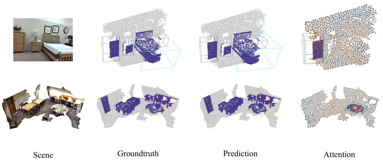
Figure 3: Qualitative results on SUN RGB-D (top) and ScanNetV2 (bottom). The color of a bounding box in the middle two columns stands for the semantic label of the object. In the last column, we draw both the groundtruth (in green) and the prediction (in blue) of the object. We highlight the points that belong to an object for better visualization. In the last column, we visualize the attention weight of the last transformer layer (before applying Local-A). We visualize the cross-attention weight between an object candidate and the point cloud.

In Figure 3, we provide qualitative results on both datasets. The visualized results are of our methods applied to the Group-Free detectors. The qualitative results suggest that our model is able to detect and classify objects of different scales even in complex scenarios containing more than 10 objects (e.g., the example in the bottom row). By looking into cross-attention weights in the transformer detector, we find that object candidates tend to have higher correlations with points that belong to their corresponding objects.

4.3 Performance on objects of different sizes.

In addition to the standard evaluation metrics, we are interested in examining models’ performance across different object sizes. Inspired by the size-aware metrics in 2D detection [12], we implement our own version of size-aware metrics for 3D detection. We conduct this analysis on ScanNetV2, on which we calculate the volume for all the objects in all samples. We set the threshold for mAP_S as the 30$th$ percentile of the volume of all objects, and use the 70$th$ percentile as the threshold for mAP_L. More details about these metrics are included in Appendix A.2.

MS-A	Local-A	mAPS	mAPM	mAPL
-	-	63.1	76.6	83.2
✔	-	65.0	77.5	83.9
-	✔	65.2	78.6	83.9
✔	✔	65.6 ($\uparrow 2.5$)	79.0 ($\uparrow 2.4$)	84.3 ($\uparrow 1.1$)

Table 3: Performance on different size categories on ScanNetV2. We define the S/M/L thresholds based on the statistics (volume distribution) of ScanNetV2 objects. The configuration in the first row denotes the Group-Free^12,512 baseline.

In Table 3, we evaluate our methods using size-aware metrics. We report the average result over 25 trials. The first row denotes the Group-Free^12,512 baseline. Firstly, by comparing the mAP_S to mAP_L, we notice that it has imbalanced performance across different object sizes. Looking at the improvement margins, we find our method to have the most performance gain on small and medium-sized objects. The result suggests that hierarchical designs can aid fine-grained and localized feature learning for point cloud transformer detectors and helps models detect smaller objects.

4.4 Ablation Study

In this subsection, we first conduct an ablation study on the stand-alone effects of our multi-scale attention and size-adaptive local attention. Next, we include empirical analyses of the design choices of our attention modules. If not otherwise specified, experiments in this subsection are conducted on ScanNetV2 with the Group-Free^12,512 baseline. Without loss of generality, the results in this subsection are the averaged numbers over 25 trials.

The stand-alone effects of MS-A and Local-A.

Table 4 shows the stand-alone performance of our proposed attention modules. Compared to the plain attention baseline, both of our attentions are proved to be effective. When combined together, we find the two modules to be complementary to each other and bring more significant performance gain.

MS-A	Local-A	mAP@0.25	mAP@0.50
-	-	68.6	51.8
✔	-	68.9	52.5
-	✔	68.9	52.9
✔	✔	69.2	53.2

Table 4: The stand-alone effect of our attention modules. The configuration in the first row denotes the Group-Free^12,512 baseline. The results are averaged over 25 trials.

The maximum number of points ($N_{local}$) in Local-A.

In Local-A, for each object candidate (i.e., query), we sample a set of points within its corresponding bounding box proposal and use the point features as the key and value for this object candidate in the cross-attention function. As introduced in Section 3.3, we cap the number of sampled points with $N_{local}$ to allow batch computation.

$N_{local}$	mAP@0.25	mAP@0.50	mAPS	mAPM	mAPL
8	67.8	51.1	64.6	78.0	82.8
16	68.9	52.9	65.2	78.6	83.9
24	68.9	53.0	65.4	78.5	84.0
32	68.3	52.1	64.7	77.8	84.3

Table 5: The effect of $N_{l}ocal$ in Local-A. When there are enough points, a larger $N_{l}ocal$ means the points are sampled more densely within each bounding box proposal.

We provide an empirical analysis of the effects of $N_{local}$ on Local-A. From Table 5, we find that too little number of points (e.g., $N_{local}=8$) for Local-A results in a performance drop. On the other hand, as $N_{local}$ continues to increase, we do not observe a significant performance gain compared to $N_{local}=16$. Intuitively, a small $N_{local}$ means the points within each bounding box are sampled sparsely, which can be too sparse to provide enough information about any object. This explains why $N_{local}=8$ does not work well. However, on the other hand, a large $N_{local}$ may only benefit large objects and has little effect on smaller objects, because the latter are padded with unused tokens.

MS-A with different feature resolutions.

In Section 3, we propose learnable upsampling for MS-A to build higher-resolution point features from the single-scale input. In the same spirit, a parameterized downsampling procedure can be realized through conventional set abstraction [23], which aggregated point features within local groups and produce a feature map with fewer points (i.e., lower resolution). Intuitively, a higher point density of the feature map provides more fine-grained features. To study the effects of feature maps of different granularity, we conduct an empirical analysis on MS-A using different sets of multi-scale feature maps representing point clouds of varying granularity.

Feature Scales $s$	mAP@0.25	mAP@0.50
$[1\times]$	68.6	51.8
$[1\times,2\times]$	68.9	52.5
$[0.5\times,1\times,2\times]$	67.9	51.7

Table 6: Simple Multi-Scale Attention with different feature scales. Feature scale $=s\times$ means the feature map contains $s\times N$ points, with $N$ being the original number of points. A larger $s$ denotes a feature map with higher point density (i.e., resolution)

In Table 6, we examined the performance of two multi-scale choices in comparison with the single-scale baseline. The result suggests that coarse features ($s=0.5\times$) do not benefit transformer detectors. This is expected because transformers do not have limited receptive fields and thus do not rely on a coarse-grained feature map to learn global context.

5 Conclusion

In this work, we present Simple Multi-Scale Attention and Size-Adaptive Local Attention, two model-agnostic modules that bring in hierarchical designs to existing transformer-based 3D detectors. We enable multi-scale feature learning and explicit localized feature aggregation through improved attention functions, which are generic modules that can be applied to any existing attention-based network for end-to-end training. We improve the state-of-the-art transformer detector on two challenging indoor 3D detection benchmarks, with the largest improvement margin on small objects.

As our attention modules promote fine-grained feature learning, which is important to various dense prediction vision tasks, one direction for future work is to adapt our attention modules for other point cloud learning problems such as segmentation. Another direction is to introduce more efficient attention mechanisms to the multi-scale attention to further bring down the computation overhead.

Appendix A Appendix

A.1 More Experiments

The placement of Simple Multi-scale Attention.

We design simple multi-scale attention as a compact network layer to enable hierarchical feature learning. As it can be inserted at any place within a network, we are interested in finding out how the placement of the multi-scale attention layer affects a model’s performance.

Layers	mAP@0.25	mAP@0.25
$[0]$	68.9	52.5
$[0,4,8]$	68.8	52.4
$[0,3,6,9]$	68.9	52.3
$[0,2,4,6,8,10]$	68.7	52.6

Table 7: Different placements of the simple multi-scale attention layer. Layers = $[i]$ means we replace the $i$th layer of the transformer decoder with our MS-A layer. The best results are in bold, and the second-best results are underlined.

We consider different strategies to place MS-A within the transformer decoder of Group-Free. We divide the 12-layer decoder into several stages and place MS-A at the first layer of each stage. Specifically, our default setting uses a single MS-A at the first decoder layer, and we try placing MS-A by dividing the decoder evenly into 3, 4, and 6 stages. From the results in Table 7, we do not observe a significant benefit of using more than one multi-scale layer. We conjecture this is because the up-scaled feature map in our multi-scale attention is obtained through interpolation and simple linear projection. The up-scale point feature obtained in this way may mainly provide more accurate geometric information with a higher point density, while may not have much semantic difference than the original input feature. We expect such fine-grained geometric information to be particularly helpful at the beginning of the decoding stage (i.e., Layer$=0$), yet may be less useful as the object features go deeper in the decoder and become more abstract.

Per-category mAP on ScanNetV2 and SUN RGB-D.

We include the detailed per-category mAP on both datasets in Table 9, Table 10, Table 11, and Table 12. For the results in this paragraph, we follow the baselines [19, 16, 27, 20] and report the result of the best trial.

Inference Speed.

We analyze the parameter and computation overhead of each of our attention modules. We measure the inference speeds for all model configurations on the same machine with a single A100 GPU. In Table 8, we can see that replacing plain attention with MS-A results in little parameter increase. While applying Local-A leads to a larger parameter increase, the Local-A module itself contains the same number of parameters as a plain cross-attention. The parameter increase is mainly due to the additional feed-forward layer and learnable positional embeddings, etc. In terms of inference speed, we find MS-A to cause more substantial latency in inference. Such latency is caused by applying the attention function on the key/value with 2 times more tokens (from 1024 to 2048). A future direction is to incorporate more efficient attention mechanisms into the multi-scale attention function.

MS-A	Local-A	#Params	Inference Speed
		(M)	(ms/frame)
-	-	26.9	186
✔	-	27.0 (+0.1)	225
-	✔	28.8 (+1.9)	191
✔	✔	28.9 (+2.0)	232

Table 8: Ablating the parameter and computation overhead of individual attention modules.

A.2 Implementation Details.

We include implementation details covering several aspects in this paragraph. In addition, we include our source code in the supplementary material, containing the full implementation of our attention modules.

Training Details.

Group-Free baseline. When applying our method to this baseline, we follow the original training settings. Specifically, on ScanNetV2, the models are trained for 400 epochs on 4 GPUs with a batchsize of 32 (8 on each GPU). We use the same optimizer with the same learning rates and weight decays as the baseline training. On SUN RGB-D, models are trained for 600 epochs on 4 GPUs with the same learning rate and weight decay as the baseline training on this dataset.

RepSurf-U baseline. The official implementation and training details of this baseline are not published. We implement our own version of RepSurf-U detector, for which we mostly follow the training setup of Group-Free and have done a grid search for the hyperparameters. Different from Group-Free, we train RepSurf-U models on ScanNetV2 and SUN RGB-D using a weight decay of 0.01 for all model parameters, because we find it to achieve better performance on our reproduced RepSurf-U. The learning rate and other hyperparameters remain the same as Group-Free on both datasets. When applying our method to the reproduced model, we do not change the hyperparameter configurations.

Bounding box parameterization.

In this paragraph, we include a brief introduction to the bounding box parameterization used in our baselines. First, the predicted box center $\mathbf{\hat{c}}$ for each object candidate $\mathbf{q}$ is obtained by adding an offset to the coordinate of $\mathbf{q}$. In this way, by predicting the center, the actual prediction made by a detector is this offset value. The size $\mathbf{\hat{d}}$ of a box is the height, width, and depth dimension. One way for predicting $\mathbf{\hat{d}}$ is to directly predict the values of H, W, and D. Another way is to divide a range of sizes into several bins and make a classification prediction that determines which “bin" the object belongs to. The final size prediction is obtained by adding the quantized size (i.e., the bin) with a “residual" term which is also predicted by the model with another prediction head. The bounding box orientation $\mathbf{\hat{a}}$ is also parameterized as the combination of a quantized value and a residual term. Lastly, the prediction of the semantic label is a common classification problem that parameterizes a semantic label as a one-hot vector.

Size-Aware Evaluation Metrics.

For a quantitative analysis of the model’s performance on objects of different sizes. We implement our own size-aware evaluation metrics, namely mAP_S, mAP_M and mAP_L. For each metric, we only calculate the mAP score among objects that fall into the corresponding size category (i.e., small, medium, or large). We conduct the size-aware evaluation on ScanNetV2, where we determine the threshold for dividing object size categories based on the statistics of this dataset. Specifically, we take the 1201 training samples and record the volume ($v=H\times W\times D$) of every groundtruth bounding box of every sample (see Figure 4). Among a total of 15733 goundtruth bounding boxes, we take the 30$th$ ($v=0.155$) and 70$th$ ($v=0.526$) percentile as the thresholds for dividing small and large objects.

Figure 4: Volume distribution of the object groundtruth bounding boxes in ScanNetV2. We highlight the threshold of small objects ($v<=0.155$, the 30$th$ percentile) and large objects ($v>0.526$, the 70$th$ percentile)

methods	backbone	cab	bed	chair	sofa	tabl	door	wind	bkshf	pic	cntr	desk	curt	fridg	showr	toil	sink	bath	ofurn	mAP
VoteNet [21]	PointNet++	47.7	88.7	89.5	89.3	62.1	54.1	40.8	54.3	12.0	63.9	69.4	52.0	52.5	73.3	95.9	52.0	92.5	42.4	62.9
H3DNet [54]	4$\times$PointNet++	49.4	88.6	91.8	90.2	64.9	61.0	51.9	54.9	18.6	62.0	75.9	57.3	57.2	75.3	97.9	67.4	92.5	53.6	67.2
3DETR [19]	transformer	49.4	83.6	90.9	89.8	67.6	52.4	39.6	56.4	15.2	55.9	79.2	58.3	57.6	67.6	97.2	70.6	92.2	53.0	65.0
Pointformer [20]	Pointformer	46.7	88.4	90.5	88.7	65.7	55.0	47.7	55.8	18.0	63.8	69.1	55.4	48.5	66.2	98.9	61.5	86.7	47.4	64.1
GroupFree6,256	PointNet++	54.1	86.2	92.0	84.8	67.8	55.8	46.9	48.5	15.0	59.4	80.4	64.2	57.2	76.3	97.6	76.8	92.5	55.0	67.3
w/ MS + Local	PointNet++	55.9	88.6	93.6	90.8	68.2	59.0	44.2	50.3	14.6	63.0	85.0	62.8	58.5	68.6	97.6	73.2	92.4	56.4	67.9
RepSurf-U6,256	PointNet++	55.5	87.7	93.4	85.9	69.1	57.3	48.8	50.0	16.5	61.0	81.6	66.2	59.0	77.5	99.2	78.2	94.0	56.8	68.8
RepSurf-U6,256 (repd.)	PointNet++	57.4	89.6	93.2	87.4	70.2	58.8	46.6	47.4	18.1	63.4	78.2	70.4	46.5	81.0	99.8	69.4	90.8	55.5	68.0
w/ MS + Local	PointNet++	51.2	89.5	93.4	87.5	71.8	60.5	49.0	57.7	21.9	65.2	82.1	70.3	53.3	80.2	98.2	68.8	91.9	58.2	69.5
GroupFree12,512	PointNet++w2x	52.1	91.9	93.6	88.0	70.7	60.7	53.7	62.4	16.1	58.5	80.9	67.9	47.0	76.3	99.6	72.0	95.3	56.4	69.1
w/ MS + Local	PointNet++	53.7	91.9	93.4	88.8	72.1	61.3	52.8	58.6	17.4	70.8	83.3	69.9	56.5	75.6	98.5	70.3	94.4	56.9	70.3
RepSurf-U12,512	PointNet++w2x	54.6	94.0	96.2	90.5	73.2	62.7	55.7	64.5	18.6	60.9	83.1	69.9	49.4	78.4	99.4	74.5	97.6	58.3	71.2
RepSurf-U12,512 (repd.)	PointNet++w2x	54.5	90.7	93.4	87.6	76.3	64.4	54.4	61.4	19.0	62.2	84.0	69.2	48.8	79.2	99.8	75.9	92.2	62.0	70.8
w/ MS + Local	PointNet++w2x	58.0	89.3	94.1	86.5	74.3	62.4	60.2	57.9	21.7	67.9	85.3	74.4	53.5	75.9	99.6	74.6	91.6	63.7	71.7

Table 9: Performance of mAP@0.25 in each category on ScanNetV2.

methods	backbone	cab	bed	chair	sofa	tabl	door	wind	bkshf	pic	cntr	desk	curt	fridg	showr	toil	sink	bath	ofurn	mAP
VoteNet [21]	PointNet++	14.6	77.8	73.1	80.5	46.5	25.1	16.0	41.8	2.5	22.3	33.3	25.0	31.0	17.6	87.8	23.0	81.6	18.7	39.9
H3DNet [54]	4$\times$PointNet++	20.5	79.7	80.1	79.6	56.2	29.0	21.3	45.5	4.2	33.5	50.6	37.3	41.4	37.0	89.1	35.1	90.2	35.4	48.1
GroupFree6,256	PointNet++	23.0	78.4	78.9	68.7	55.1	35.3	23.6	39.4	7.5	27.2	66.4	43.3	43.0	41.2	89.7	38.0	83.4	37.3	48.9
w/ MS + Local	PointNet++	27.3	80.8	83.3	85.3	60.2	39.7	21.7	40.4	7.6	41.7	61.5	42.9	42.3	26.2	96.1	38.5	89.5	39.7	51.4
RepSurf-U6,256	PointNet++	24.9	79.6	80.1	70.4	56.4	36.7	25.5	41.4	8.8	28.7	68.0	45.2	45.0	42.7	91.3	40.1	85.1	39.2	50.5
RepSurf-U6,256 (repd.)	PointNet++ 1.	24.3	82.6	82.6	71.3	55.9	38.3	18.6	40.3	11.2	44.0	60.7	45.1	35.7	36.6	97.1	34.6	84.6	39.8	50.2
w/ MS + Local	PointNet++	27.1	80.9	83.0	77.1	58.0	45.8	24.8	50.8	10.5	31.9	67.7	44.6	40.6	34.9	97.7	38.3	87.3	44.6	52.5
GroupFree12,512	PointNet++w2x	26.0	81.3	82.9	70.7	62.2	41.7	26.5	55.8	7.8	34.7	67.2	43.9	44.3	44.1	92.8	37.4	89.7	40.6	52.8
w/ MS + Local	PointNet++	31.0	81.0	85.0	79.4	61.1	44.5	27.9	50.6	10.1	45.0	61.2	54.1	39.5	43.5	91.7	45.9	89.3	42.4	54.6
RepSurf-U12,512	PointNet++w2x	28.5	83.5	84.8	72.6	64.0	43.6	28.3	57.8	9.6	37.0	69.7	45.9	46.4	46.1	94.9	39.1	92.1	42.6	54.8
RepSurf-U12,512 (repd.)	PointNet++w2x	27.6	82.7	85.3	68.8	60.6	44.0	27.3	56.7	9.6	39.6	63.7	53.8	43.0	42.4	99.8	38.8	88.7	47.3	54.4
w/ MS + Local	PointNet++w2x	29.3	83.6	85.7	78.7	66.2	45.6	30.4	59.8	10.4	34.2	60.0	60.8	48.1	45.3	99.9	44.5	87.1	48.4	56.5

Table 10: Performance of mAP@0.50 in each category on ScanNetV2.

methods	backbone	bathtub	bed	bkshf	chair	desk	drser	nigtstd	sofa	table	toilet	mAP
VoteNet [21]	PointNet++	75.5	85.6	31.9	77.4	24.8	27.9	58.6	67.4	51.1	90.5	59.1
H3DNet [54]	4$\times$PointNet++	73.8	85.6	31.0	76.7	29.6	33.4	65.5	66.5	50.8	88.2	60.1
3DETR [19]	transformer	69.8	84.6	28.5	72.4	34.3	29.6	61.4	65.3	52.6	91.0	61.1
Pointformer [20]	Pointformer	80.1	84.3	32.0	76.2	27.0	37.4	64.0	64.9	51.5	92.2	61.1
GroupFree6,256	PointNet++	80.0	87.8	32.5	79.4	32.6	36.0	66.7	70.0	53.8	91.1	63.0
w/ MS + Local	PointNet++	83.2	86.7	34.5	79.0	31.9	39.3	66.0	70.6	55.6	90.8	63.8
RepSurf-U6,256	PointNet++	81.1	89.3	34.4	80.4	33.5	37.3	68.1	71.4	54.8	92.3	64.3
RepSurf-U6,256 (repd.)	PointNet++	79.5	87.5	33.8	79.4	32.7	40.2	69.0	70.3	55.4	92.1	64.0
w/ MS + Local	PointNet++	79.9	87.0	36.8	79.5	33.8	41.4	67.4	71.2	55.3	92.4	64.5

Table 11: Performance of mAP@0.25 in each category on SUN RGB-D.

methods	backbone	bathtub	bed	bkshf	chair	desk	drser	nigtstd	sofa	table	toilet	mAP
VoteNet [21]	PointNet++	45.4	53.4	6.8	56.5	5.9	12.0	38.6	49.1	21.3	68.5	35.8
H3DNet [54]	4$\times$PointNet++	47.6	52.9	8.6	60.1	8.4	20.6	45.6	50.4	27.1	69.1	39.0
GroupFree6,256	PointNet++	64.0	67.1	12.4	62.6	14.5	21.9	49.8	58.2	29.2	72.2	45.2
w/ MS + Local	PointNet++	66.2	67.4	10.8	63.6	15.0	24.7	56.7	56.1	30.8	74.3	46.6
RepSurf-U6,256	PointNet++	65.2	67.5	13.2	63.4	15.0	22.4	50.9	58.8	30.0	72.7	45.9
RepSurf-U6,256 (repd.)	PointNet++	61.4	66.8	11.3	64.0	14.8	24.2	51.8	59.0	31.6	71.7	45.7
w/ MS + Local	PointNet++	62.2	67.6	16.6	65.0	15.0	24.2	57.0	59.0	30.9	77.7	47.5

Table 12: Performance of mAP@0.50 in each category on SUN RGB-D.

References

- [1] Nicolas Carion, Francisco Massa, Gabriel Synnaeve, Nicolas Usunier, Alexander Kirillov, and Sergey Zagoruyko. End-to-end object detection with transformers. In ECCV, 2020.
- [2] Xiaozhi Chen, Huimin Ma, Ji Wan, Bo Li, and Tian Xia. Multi-view 3d object detection network for autonomous driving. In CVPR, 2017.
- [3] Angela Dai, Angel X. Chang, Manolis Savva, Maciej Halber, Thomas A. Funkhouser, and Matthias Nießner. Scannet: Richly-annotated 3d reconstructions of indoor scenes. In CVPR, 2017.
- [4] Jacob Devlin, Ming-Wei Chang, Kenton Lee, and Kristina Toutanova. BERT: Pre-training of Deep Bidirectional Transformers for Language Understanding. In NAACL-HLT (1), 2019.
- [5] Alexey Dosovitskiy, Lucas Beyer, Alexander Kolesnikov, Dirk Weissenborn, Xiaohua Zhai, Thomas Unterthiner, Mostafa Dehghani, Matthias Minderer, Georg Heigold, Sylvain Gelly, Jakob Uszkoreit, and Neil Houlsby. An Image is Worth 16x16 Words: Transformers for Image Recognition at Scale. In ICLR, 2021.
- [6] Haoqi Fan, Bo Xiong, Karttikeya Mangalam, Yanghao Li, Zhicheng Yan, Jitendra Malik, and Christoph Feichtenhofer. Multiscale vision transformers. In ICCV, 2021.
- [7] Benjamin Graham, Martin Engelcke, and Laurens van der Maaten. 3d semantic segmentation with submanifold sparse convolutional networks. In CVPR, 2018.
- [8] Loïc Landrieu and Martin Simonovsky. Large-scale point cloud semantic segmentation with superpoint graphs. In CVPR, 2018.
- [9] Alex H. Lang, Sourabh Vora, Holger Caesar, Lubing Zhou, Jiong Yang, and Oscar Beijbom. Pointpillars: Fast encoders for object detection from point clouds. In CVPR, 2019.
- [10] Yann LeCun, Bernhard E. Boser, John S. Denker, Donnie Henderson, Richard E. Howard, Wayne E. Hubbard, and Lawrence D. Jackel. Backpropagation applied to handwritten zip code recognition. Neural Comput., 1989.
- [11] Yanghao Li, Chao-Yuan Wu, Haoqi Fan, Karttikeya Mangalam, Bo Xiong, Jitendra Malik, and Christoph Feichtenhofer. Mvitv2: Improved multiscale vision transformers for classification and detection. In CVPR, 2022.
- [12] Tsung-Yi Lin, Michael Maire, Serge J. Belongie, James Hays, Pietro Perona, Deva Ramanan, Piotr Dollár, and C. Lawrence Zitnick. Microsoft COCO: common objects in context. In ECCV, 2014.
- [13] Wei Liu, Dragomir Anguelov, Dumitru Erhan, Christian Szegedy, Scott E. Reed, Cheng-Yang Fu, and Alexander C. Berg. SSD: single shot multibox detector. In ECCV, 2016.
- [14] Ze Liu, Yutong Lin, Yue Cao, Han Hu, Yixuan Wei, Zheng Zhang, Stephen Lin, and Baining Guo. Swin Transformer: Hierarchical Vision Transformer using Shifted Windows. In ICCV, 2021.
- [15] Ze Liu, Yutong Lin, Yue Cao, Han Hu, Yixuan Wei, Zheng Zhang, Stephen Lin, and Baining Guo. Swin transformer: Hierarchical vision transformer using shifted windows. In ICCV, 2021.
- [16] Ze Liu, Zheng Zhang, Yue Cao, Han Hu, and Xin Tong. Group-free 3d object detection via transformers. In ICCV, 2021.
- [17] Xu Ma, Can Qin, Haoxuan You, Haoxi Ran, and Yun Fu. Rethinking network design and local geometry in point cloud: A simple residual MLP framework. In ICLR, 2022.
- [18] Daniel Maturana and Sebastian Scherer. Voxnet: A 3d convolutional neural network for real-time object recognition. In 2015 IEEE/RSJ International Conference on Intelligent Robots and Systems (IROS), 2015.
- [19] Ishan Misra, Rohit Girdhar, and Armand Joulin. An end-to-end transformer model for 3d object detection. In ICCV, 2021.
- [20] Xuran Pan, Zhuofan Xia, Shiji Song, Li Erran Li, and Gao Huang. 3d object detection with pointformer. In CVPR, 2021.
- [21] Charles R. Qi, Or Litany, Kaiming He, and Leonidas J. Guibas. Deep hough voting for 3d object detection in point clouds. In ICCV, 2019.
- [22] Charles R. Qi, Wei Liu, Chenxia Wu, Hao Su, and Leonidas J. Guibas. Frustum pointnets for 3d object detection from RGB-D data. In CVPR, 2018.
- [23] Charles Ruizhongtai Qi, Hao Su, Kaichun Mo, and Leonidas J. Guibas. Pointnet: Deep learning on point sets for 3d classification and segmentation. In CVPR, 2017.
- [24] Charles Ruizhongtai Qi, Hao Su, Matthias Nießner, Angela Dai, Mengyuan Yan, and Leonidas J. Guibas. Volumetric and multi-view cnns for object classification on 3d data. In CVPR, 2016.
- [25] Charles Ruizhongtai Qi, Li Yi, Hao Su, and Leonidas J. Guibas. Pointnet++: Deep hierarchical feature learning on point sets in a metric space. In NIPS, 2017.
- [26] Colin Raffel, Noam Shazeer, Adam Roberts, Katherine Lee, Sharan Narang, Michael Matena, Yanqi Zhou, Wei Li, and Peter J. Liu. Exploring the Limits of Transfer Learning with a Unified Text-to-Text Transformer. J. Mach. Learn. Res., 21, 2020.
- [27] Haoxi Ran, Jun Liu, and Chengjie Wang. Surface representation for point clouds. In CVPR, 2022.
- [28] Joseph Redmon, Santosh Kumar Divvala, Ross B. Girshick, and Ali Farhadi. You only look once: Unified, real-time object detection. In CVPR, 2016.
- [29] Shaoqing Ren, Kaiming He, Ross B. Girshick, and Jian Sun. Faster R-CNN: towards real-time object detection with region proposal networks. In NIPS, 2015.
- [30] Sucheng Ren, Daquan Zhou, Shengfeng He, Jiashi Feng, and Xinchao Wang. Shunted self-attention via multi-scale token aggregation. In CVPR, 2022.
- [31] Gernot Riegler, Ali Osman Ulusoy, and Andreas Geiger. Octnet: Learning deep 3d representations at high resolutions. In CVPR, 2017.
- [32] Hualian Sheng, Sijia Cai, Yuan Liu, Bing Deng, Jianqiang Huang, Xian-Sheng Hua, and Min-Jian Zhao. Improving 3d object detection with channel-wise transformer. In ICCV, 2021.
- [33] Shaoshuai Shi, Chaoxu Guo, Li Jiang, Zhe Wang, Jianping Shi, Xiaogang Wang, and Hongsheng Li. PV-RCNN: point-voxel feature set abstraction for 3d object detection. In CVPR, 2020.
- [34] Shaoshuai Shi, Xiaogang Wang, and Hongsheng Li. Pointrcnn: 3d object proposal generation and detection from point cloud. In CVPR, 2019.
- [35] Martin Simonovsky and Nikos Komodakis. Dynamic edge-conditioned filters in convolutional neural networks on graphs. In CVPR, 2017.
- [36] Shuran Song, Samuel P. Lichtenberg, and Jianxiong Xiao. SUN RGB-D: A RGB-D scene understanding benchmark suite. In CVPR, 2015.
- [37] Hang Su, Varun Jampani, Deqing Sun, Subhransu Maji, Evangelos Kalogerakis, Ming-Hsuan Yang, and Jan Kautz. Splatnet: Sparse lattice networks for point cloud processing. In CVPR, 2018.
- [38] Anirud Thyagharajan, Benjamin Ummenhofer, Prashant Laddha, Om Ji Omer, and Sreenivas Subramoney. Segment-fusion: Hierarchical context fusion for robust 3d semantic segmentation. In CVPR, 2022.
- [39] Hugo Touvron, Matthieu Cord, Matthijs Douze, Francisco Massa, Alexandre Sablayrolles, and Hervé Jégou. Training data-efficient image transformers & distillation through attention. In ICML, 2021.
- [40] Ashish Vaswani, Noam Shazeer, Niki Parmar, Jakob Uszkoreit, Llion Jones, Aidan N. Gomez, Lukasz Kaiser, and Illia Polosukhin. Attention is all you need. In NLPS, 2017.
- [41] Haiyang Wang, Shaoshuai Shi, Ze Yang, Rongyao Fang, Qi Qian, Hongsheng Li, Bernt Schiele, and Liwei Wang. Rbgnet: Ray-based grouping for 3d object detection. In CVPR, 2022.
- [42] Peng-Shuai Wang, Yang Liu, Yu-Xiao Guo, Chun-Yu Sun, and Xin Tong. O-CNN: octree-based convolutional neural networks for 3d shape analysis. ACM Trans. Graph., 36(4):72:1–72:11, 2017.
- [43] Wenhai Wang, Enze Xie, Xiang Li, Deng-Ping Fan, Kaitao Song, Ding Liang, Tong Lu, Ping Luo, and Ling Shao. Pyramid vision transformer: A versatile backbone for dense prediction without convolutions. In ICCV, 2021.
- [44] Yue Wang, Yongbin Sun, Ziwei Liu, Sanjay E. Sarma, Michael M. Bronstein, and Justin M. Solomon. Dynamic graph CNN for learning on point clouds. ACM Trans. Graph., 38(5):146:1–146:12, 2019.
- [45] Qian Xie, Yu-Kun Lai, Jing Wu, Zhoutao Wang, Yiming Zhang, Kai Xu, and Jun Wang. Mlcvnet: Multi-level context votenet for 3d object detection. In CVPR, 2020.
- [46] Saining Xie, Sainan Liu, Zeyu Chen, and Zhuowen Tu. Attentional shapecontextnet for point cloud recognition. In CVPR, 2018.
- [47] Qiangeng Xu, Xudong Sun, Cho-Ying Wu, Panqu Wang, and Ulrich Neumann. Grid-gcn for fast and scalable point cloud learning. In CVPR, 2020.
- [48] Yifan Xu, Tianqi Fan, Mingye Xu, Long Zeng, and Yu Qiao. Spidercnn: Deep learning on point sets with parameterized convolutional filters. In ECCV, 2018.
- [49] Jiancheng Yang, Qiang Zhang, Bingbing Ni, Linguo Li, Jinxian Liu, Mengdie Zhou, and Qi Tian. Modeling point clouds with self-attention and gumbel subset sampling. In CVPR, 2019.
- [50] Yaoqing Yang, Chen Feng, Yiru Shen, and Dong Tian. Foldingnet: Point cloud auto-encoder via deep grid deformation. In CVPR, 2018.
- [51] Maosheng Ye, Shuangjie Xu, and Tongyi Cao. Hvnet: Hybrid voxel network for lidar based 3d object detection. In CVPR, 2020.
- [52] Xumin Yu, Lulu Tang, Yongming Rao, Tiejun Huang, Jie Zhou, and Jiwen Lu. Point-bert: Pre-training 3d point cloud transformers with masked point modeling. In CVPR, 2022.
- [53] Cheng Zhang, Haocheng Wan, Xinyi Shen, and Zizhao Wu. Patchformer: An efficient point transformer with patch attention. In CVPR, 2022.
- [54] Zaiwei Zhang, Bo Sun, Haitao Yang, and Qixing Huang. H3dnet: 3d object detection using hybrid geometric primitives. In ECCV, 2020.
- [55] Hengshuang Zhao, Li Jiang, Jiaya Jia, Philip H. S. Torr, and Vladlen Koltun. Point transformer. In ICCV, 2021.
- [56] Haoran Zhou, Yidan Feng, Mingsheng Fang, Mingqiang Wei, Jing Qin, and Tong Lu. Adaptive graph convolution for point cloud analysis. In ICCV, 2021.
- [57] Yin Zhou and Oncel Tuzel. Voxelnet: End-to-end learning for point cloud based 3d object detection. In CVPR, 2018.