Abstract

Motivated by the improved results from the HPQCD lattice collaboration on the hadronic matrix elements entering $\Delta M_{s,d}$ in $B_{s,d}^{0}-\bar{B}_{s,d}^{0}$ mixings and the increase of the experimental branching ratio for $B_{s}\to\mu^{+}\mu^{-}$, we update our 2016 analysis of various flavour observables in four 331 models, M1, M3, M13 and M16 based on the gauge group $SU(3)_{C}\times SU(3)_{L}\times U(1)_{X}$. These four models, which are distinguished by the quantum numbers, are selected among 24 331 models through their consistency with the electroweak precision tests and simultaneously by the relation $C_{9}^{\text{NP}}=-b\,C_{10}^{\text{NP}}$ with $2\leq b\leq 5$, which after new result on $B_{s}\to\mu^{+}\mu^{-}$ from CMS is favoured over the popular relation $C_{9}^{\text{NP}}=-C_{10}^{\text{NP}}$ predicted by several leptoquark models. In this context we investigate in particular the dependence of various observables on $|V_{cb}|$, varying it in the broad range $[0.0386,\,0.043]$, that encompasses both its inclusive and exclusive determinations. Imposing the experimental constraints from $\varepsilon_{K}$, $\Delta M_{s}$, $\Delta M_{d}$ and the mixing induced CP asymmetries $S_{\psi K_{S}}$ and $S_{\psi K_{S}}$, we investigate for which values of $|V_{cb}|$ the four models can be made compatible with these data and what is the impact on $B$ and $K$ branching ratios. In particular we analyse NP contributions to the Wilson coefficients $C_{9}$ and $C_{10}$ and the decays $B_{s,d}\to\mu^{+}\mu^{-}$, $K^{+}\rightarrow\pi^{+}\nu\bar{\nu}$ and $K_{L}\rightarrow\pi^{0}\nu\bar{\nu}$. This allows us to illustrate how the value of $|V_{cb}|$ determined together with other parameters of these models is infected by NP contributions and compare it with the one obtained recently under the assumption of the absence of NP in $\varepsilon_{K}$, $\Delta M_{s}$, $\Delta M_{d}$ and $S_{\psi K_{S}}$.

1 Introduction

The Standard Model (SM) describes globally the existing data on quark-flavour violating processes rather well [1] but with the reduction of experimental errors and increased precision in non-perturbative and perturbative QCD and electroweak calculations a number of tensions at the level of $2-5\,\sigma$ seem to emerge in various seemingly unrelated observables. While some of these tensions could turn out to be the result of statistical fluctuations, underestimate of systematical and theoretical errors, it is not excluded that eventually they all signal the presence of some kind of new physics (NP). Therefore, it is interesting to investigate what this NP could be.

In the present paper we will address some of these tensions in four particular 331 models based on the gauge group $SU(3)_{C}\times SU(3)_{L}\times U(1)_{X}$ [2, 3] . As these models have much smaller number of new parameters than supersymmetric models, Randall-Sundrum scenarios and Littlest Higgs models, it is not evident that they can remove all present tensions simultaneously.

Our paper has been motivated by the following recent facts.

• As demonstrated in [6] most recent lattice QCD results from HPQCD collaboration [7], based on $2+1+1$ simulations, imply simultaneous agreement of

  $$|\varepsilon_{K}|,\qquad\Delta M_{s},\qquad\Delta M_{d},\qquad S_{\psi K_{S}}\,\qquad S_{\psi\phi}$$ (1)

  within the SM with the data for rather precise values of $|V_{cb}|$, $|V_{ub}|$ and $\gamma$. This should be contrasted with the situation at the time of our previous analysis 2016 [8], when significant tensions between $\varepsilon_{K}$ and $\Delta M_{s,d}$ within the SM have been found [9] and the room for NP in the quark mixing sector was much larger than it is now.

• The most recent data on $B_{s}\to\mu^{+}\mu^{-}$ from CMS imply that in the case of the dominance of left-handed quark currents, as is the case of the 331 models, roughly [10]

  $$C_{9}^{\text{NP}}=-b\,C_{10}^{\text{NP}},\qquad{2\leq b\leq 5},$$ (2)

  where $C_{9}^{\text{NP}},\,C_{10}^{\text{NP}}$ represent the shifts in the Wilson coefficients $C_{9},\,C_{10}$ of the $b\to s\ell^{+}\ell^{-}$ effective Hamiltonian in the presence of NP. The relation (2) is in contrast to the previously favoured case $b=1$ found in several leptoquark models, in particular in the $U_{1}$ model.

• Recent messages from the LHCb [11, 12], that the lepton flavour universality violation (LFUV) in $b\to s\ell^{+}\ell^{-}$, which for many years dominated the $B$-physics anomalies, practically disappeared. This is good news for 331 models for which LFUV anomalies were problematic, although these models could provide some shifts in the Wilson coefficients $C_{9}$ and $C_{10}$. Such shifts, in particular in $C_{9}$, are still required to describe suppressed branching ratios in $b\to s\mu^{+}\mu^{-}$ transitions.

• The most recent value for $\gamma$ obtained by the LHCb collaboration from tree-level decays that reads [13]

  $$\gamma=(63.8^{+3.5}_{-3.7})^{\circ}\,.$$ (3)

  It is significantly more precise than the LHCb values of $\gamma$ in 2016 that could be as large as $75^{\circ}$.

The question then arises how 331 models face this new situation relative to the 2016 input and what are the implications for many flavour observables, in particular for the decays $B_{d}\to K(K^{*})\mu^{+}\mu^{-}$, $B^{+}\to K^{+}\mu^{+}\mu^{-}$ and $B_{s}\to\phi\mu^{+}\mu^{-}$ related to the $B$ physics anomalies that imply the need for significant NP contributions to the Wilson coefficient $C_{9}$ and smaller to $C_{10}$. But it is also of interest to see what are the implications for rare decays $B_{s,d}\to\mu^{+}\mu^{-}$, $K^{+}\rightarrow\pi^{+}\nu\bar{\nu}$ and $K_{L}\rightarrow\pi^{0}\nu\bar{\nu}$.

It is known from many analyses, and stressed recently in particular in [14, 6] that the tensions between inclusive and exclusive determinations of $|V_{cb}|$ and $|V_{ub}|$ preclude precise predictions for rare decay observables in the SM. However, eliminating these parameters with the help of $\varepsilon_{K}$, $\Delta M_{s,d}$ and $S_{\psi K_{S}}$ and setting the latter observables to their experimental values allowed to obtain SM predictions for many flavour observables that are most precise to date [14, 6]. The motivation for this strategy has been strengthened recently by one of us [15] as the one which could minimize the impact of NP on the determination of the CKM parameters. Indeed, as demonstrated in [6], presently no NP is required to describe precise experimental data on $\Delta F=2$ observables. This allows in turn to determine the CKM parameters on the basis of $\Delta F=2$ observables alone without being involved in the issue of $|V_{cb}|$ and $|V_{ub}|$ tensions and minimizing possible impact of NP on their values that otherwise would infect SM predictions for rare decay branching ratios.

The resulting values of the CKM parameters read [6]

$$\boxed{|V_{cb}|=42.6(4)\times 10^{-3},\qquad|V_{ub}|=3.72(11)\times 10^{-3},\qquad\gamma=64.6(16)^{\circ}.}$$ (4)

While in this manner one can obtain rather precise SM predictions for numerous branching ratios [14, 6, 15], the absence of NP in the $\Delta F=2$ observables, if confirmed with higher precision, would be a nightmare scenario for many NP models that attempt to explain the $B$ physics anomalies. While the ones related to lepton flavour universality violation have been dwarfed recently through new LHCb data [11, 12], sizeable anomalies remained in several branching ratios. In particular using the strategy of [14, 6] large anomalies in the low $q^{2}$ bin in $B^{+}\to K^{+}\mu^{+}\mu^{-}$ ($5.1\sigma$) and $B_{s}\to\phi\mu^{+}\mu^{-}$ ($4.8\sigma$) have been found [15].

Explaining such anomalies without practically no NP contributions to $\Delta F=2$ processes is in principle possible but would require significant tuning of NP parameters. Now, the value of $\gamma$ in (4) agrees very well with the most recent value from LHCb in (3) and experimental value of $\beta$ from $S_{\psi K_{S}}$ is already used in obtaining the CKM parameters in (4). It is evident then that the most efficient and transparent strategy to allow NP to enter the $\Delta F=2$ sector is to modify the value of $|V_{cb}|$.

In this context in [6], two scenarios for the parameters $|V_{cb}|$ and $|V_{ub}|$ have been analysed within the SM. The EXCLUSIVE one based on determinations of these parameters in exclusive decays

$$|V_{cb}|=39.21(62)\times 10^{-3},\qquad|V_{ub}|=3.61(13)\times 10^{-3},\qquad{(\rm EXCLUSIVE)},$$ (5)

and the HYBRID scenario in which the value for $|V_{cb}|$ is the inclusive one from [16] and the exclusive one for $|V_{ub}|$ as above:

$${|V_{cb}|=42.16(50)\times 10^{-3},\qquad|V_{ub}|=3.61(13)\times 10^{-3},\qquad{(\rm HYBRID)}.}$$ (6)

Decay	EXCLUSIVE	HYBRID	DATA
$\mathcal{B}(K^{+}\rightarrow\pi^{+}\nu\bar{\nu})\times 10^{11}$	$6.88(38)$	$8.44(41)$	$10.9(38)$ [17]
$\mathcal{B}(K_{L}\rightarrow\pi^{0}\nu\bar{\nu})\times 10^{11}$	$2.37(15)$	$2.74(14)$	$<300$ [18]
$\mathcal{B}(K_{S}\to\mu^{+}\mu^{-})\times 10^{13}_{\text{SD}}$	$1.49(10)$	$1.72(8)$	$<0.8~{}10^{4}$ [19]
$\overline{\mathcal{B}}(B_{s}\to\mu^{+}\mu^{-})\times 10^{9}$	$3.18(12)$	$3.67(12)$	$3.45(29)$ [20, 21, 22, 23]
$\mathcal{B}(B_{d}\to\mu^{+}\mu^{-})\times 10^{10}$	$0.864(34)$	$0.999(34)$	$<2.05$ [20]
$|\varepsilon_{K}|\times 10^{3}$	$1.78(11)$	$2.14(12)$	$2.228(11)$ [24]
$S_{\psi K_{S}}$	$0.731(24)$	$0.688(22)$	$0.699(17)$ [24]
$\Delta M_{s}\,\text{ps}^{-1}$	$15.02(87)$	$17.35(94)$	$17.749(20)$ [24]
$\Delta M_{d}\,\text{ps}^{-1}$	$0.434(28)$	$0.502(31)$	$0.5065(19)$ [24]

Table 1: Predictions (second column) for selected observables within the SM obtained in [6] using the EXCLUSIVE strategy for $|V_{cb}|$ and $|V_{ub}|$ and $\gamma=65.4^{\circ}$. In the third column we show the results for the HYBRID choice of $|V_{cb}|$ and $|V_{ub}|$ as given in (6) and in the fourth the experimental data.

In Table 1 we show selected results obtained in [6] in these two scenarios. The results obtained in the HYBRID scenario do not differ by much from those obtained using the CKM parameters in (4) [6, 15]. With exclusive values of $|V_{cb}|$ that are much lower than given in (4), anomalies in $\Delta M_{s}$ ($3\sigma$), $\Delta M_{d}$ ($4\sigma$) and $\varepsilon_{K}$ ($5\sigma$) are generated. But in [6] no analysis of a NP scenario has been presented which would explain these anomalies and whether a model explaining them would also be able to explain anomalies in semi-leptonic B decays. In the present paper we investigate whether the 331 models could provide some insight in these issues and what would be the implications for rare branching ratios. Our analysis illustrates in simple settings how the determination of $|V_{cb}|$ in a global fit that includes observables exposing anomalies can be infected by NP contributions [15]. Indeed the allowed values of $|V_{cb}|$ depend on the 331 model considered. It is a concrete illustration of the points made in section 2 of the latter paper.

Our paper is organized as follows. In Section 2 we recall briefly the flavour structure of the 331 models. In Section 3 we select four 331 models that perform best on the basis of electroweak precision tests and the present experimental values of the ratio $C_{9}^{\text{NP}}/C_{10}^{\text{NP}}$ in (2). In fact these are the only models among the 24 ones considered in [25], that can successfully face the new relation (2) when other constraints like electroweak precision tests are taken into account [8]. In Section 4 we present numerical analysis of these models addressing the issues mentioned above. We conclude in Section 5.

2 Flavour Structure of 331 Models

Let us recall that in the 331 models new flavour-violating effects are governed by tree-level $Z^{\prime}$ exchanges with a subdominant but non-negligible role played by tree-level $Z$ exchanges generated through $Z-Z^{\prime}$ mixing. All the formulae for flavour observables in these models can be found in [26, 27, 25, 28] and will not be repeated here. In particular the collection of formulae for $Z^{\prime}$ couplings to quarks and leptons are given in [27].

New sources of flavour and CP violation in 331 models are parametrized by new mixing parameters and phases

$$\tilde{s}_{13},\qquad\tilde{s}_{23},\qquad\delta_{1},\qquad\delta_{2}$$ (7)

with $\tilde{s}_{13}$ and $\tilde{s}_{23}$ positive definite and smaller than unity and $0\leq\delta_{1,2}\leq 2\pi$. They can be constrained by flavour observables as demonstrated in detail in [26]. The non-diagonal $Z^{\prime}$ couplings relevant for $K$, $B_{d}$ and $B_{s}$ meson systems can be then parametrized respectively within an excellent approximation through

$$v_{32}^{*}v_{31}=\tilde{s}_{13}\tilde{s}_{23}e^{i(\delta_{2}-\delta_{1})},\qquad v_{33}^{*}v_{31}=-\tilde{s}_{13}e^{-i\delta_{1}},\qquad v_{33}^{*}v_{32}=-\tilde{s}_{23}e^{-i\delta_{2}}\,.$$ (8)

$\tilde{s}_{13}$ and $\delta_{1}$ can be determined from $\Delta M_{d}$ and CP-asymmetry $S_{\psi K_{S}}$ while $\tilde{s}_{23}$ and $\delta_{2}$ from $\Delta M_{s}$ and CP-asymmetry $S_{\psi\phi}$. Then the parameters in the $K$ system are fixed. It is a remarkable feature of 331 models that also FCNC processes in the charm sector can be described without introducing no new free parameters beyond those already present in the beauty and kaon meson systems [29, 30]. These correlations constitute important tests of these models.

The remaining two parameters, except for $M_{Z^{\prime}}$ mass, are $\beta$ and $\tan\bar{\beta}$ defined through

$$Q=T_{3}+\frac{Y}{2}=T_{3}+\beta T_{8}+X,\qquad\tan\bar{\beta}=\frac{v_{\rho}}{v_{\eta}}\,.$$ (9)

Here $T_{3,8}$ and $X$ are the diagonal generators of $SU(3)_{L}$ and $U(1)_{X}$, respectively. $Y$ represents $U(1)_{Y}$ and $v_{i}$ are the vacuum expectation values of scalar triplets responsible for the generation of down- and up-quark masses in these models.

Different 331 models can also be distinguished by the way quarks transform under $SU(3)_{L}$. In [25] two classes of such models have been analyzed to be denoted by $F_{1}$ and $F_{2}$. $F_{1}$ stands for the case in which the first two generations of quarks belong to triplets of $SU(3)_{L}$, while the third generation of quarks to antitriplet. $F_{2}$ stands for the case in which the first two generations of quarks belong to antitriplets of $SU(3)_{L}$, while the third generation of quarks to triplet.

A detailed analysis of 24 331 models corresponding to different values of $\beta$ and $\tan\bar{\beta}$ for the representations $F_{1}$ and $F_{2}$ has been presented in [25]. They are collected in Table 2. With the values of $\beta$ and $\tan\bar{\beta}$ being fixed, flavour phenomenology depends only on the parameters in (7), $M_{Z^{\prime}}$ and the CKM parameters which distinguish EXCLUSIVE and HYBRID scenarios.

3 Selecting the 331 Models

A detailed analysis of electroweak precision tests in the 24 models in Table 2 has been performed in [25]. Interested readers are asked to look at Section 5 of that paper. Here we just summarize the main outcome of that study.

Requiring that the 24 models in question perform well in these tests and are simultaneously consistent with the ratio $C_{9}/C_{10}$ in (2) selects, as shown in Table 3, the following models

$${\rm M1},\qquad{\rm M3},\qquad{\rm M13},\qquad{\rm M16},\qquad{(\rm favoured)}.$$ (10)

Note that the $Z-Z^{\prime}$ mixing plays in some cases an important role and that the two favoured models M8 and M9 analysed by us in [8] are ruled out by (2).

MI	scen.	$\beta$	$\tan{\bar{\beta}}$	MI	scen.	$\beta$	$\tan{\bar{\beta}}$	MI	scen.	$\beta$	$\tan{\bar{\beta}}$
M1	$F_{1}$	$-2/\sqrt{3}$	1	M9	$F_{2}$	$-2/\sqrt{3}$	1	M17	$F_{1}$	$-2/\sqrt{3}$	0.2
M2	$F_{1}$	$-2/\sqrt{3}$	5	M10	$F_{2}$	$-2/\sqrt{3}$	5	M18	$F_{2}$	$-2/\sqrt{3}$	0.2
M3	$F_{1}$	$-1/\sqrt{3}$	1	M11	$F_{2}$	$-1/\sqrt{3}$	1	M19	$F_{1}$	$-1/\sqrt{3}$	0.2
M4	$F_{1}$	$-1/\sqrt{3}$	5	M12	$F_{2}$	$-1/\sqrt{3}$	5	M20	$F_{2}$	$-1/\sqrt{3}$	0.2
M5	$F_{1}$	$1/\sqrt{3}$	1	M13	$F_{2}$	$1/\sqrt{3}$	1	M21	$F_{1}$	$1/\sqrt{3}$	0.2
M6	$F_{1}$	$1/\sqrt{3}$	5	M14	$F_{2}$	$1/\sqrt{3}$	5	M22	$F_{2}$	$1/\sqrt{3}$	0.2
M7	$F_{1}$	$2/\sqrt{3}$	1	M15	$F_{2}$	$2/\sqrt{3}$	1	M23	$F_{1}$	$2/\sqrt{3}$	0.2
M8	$F_{1}$	$2/\sqrt{3}$	5	M16	$F_{2}$	$2/\sqrt{3}$	5	M24	$F_{2}$	$2/\sqrt{3}$	0.2

Table 2: Definition of the various 331 models.

 

MI	Full	no Mixing	MI	Full	no Mixing	MI	Full	no Mixing
M1	$-3.25$	$-8.87$	M9	$0.42$	$0.60$	M17	$-175.6$	$-8.87$
M2	$-1.68$	$-8.87$	M10	$0.28$	$0.60$	M18	$0.75$	$0.60$
M3	$-2.07$	$-2.98$	M11	$-0.02$	$-0.004$	M19	$-63.48$	$-2.98$
M4	$-1.09$	$-2.98$	M12	$-0.04$	$-0.004$	M20	$0.06$	$-0.004$
M5	$0.02$	$-0.004$	M13	$-5.47$	$-2.98$	M21	$1.15$	$-0.004$
M6	$-0.03$	$-0.004$	M14	$-1.56$	$-2.98$	M22	$3.25$	$-2.98$
M7	$0.97$	$0.60$	M15	$11.3$	$-8.87$	M23	$7.50$	$0.60$
M8	$0.49$	$0.60$	M16	$-4.59$	$-8.87$	M24	$2.44$	$-8.87$

Table 3: $C_{9}^{\text{NP}}/C_{10}^{\text{NP}}$ in various 331 models with and without $Z-Z^{\prime}$ mixing for $M_{Z^{\prime}}=3\,{\rm TeV}$.

 

4 Numerical Analysis

$m_{B_{s}}=5366.8(2)\,{\rm MeV}$ [24]	$m_{B_{d}}=5279.58(17)\,{\rm MeV}$ [24]
$\Delta M_{s}=17.749(20)\,\text{ps}^{-1}$ [24]	$\Delta M_{d}=0.5065(19)\,\text{ps}^{-1}$ [24]
$\Delta M_{K}=0.005292(9)\,\text{ps}^{-1}$ [24]	$m_{K^{0}}=497.61(1)\,{\rm MeV}$ [24]
$S_{\psi K_{S}}=0.699(17)$ [24]	$F_{K}=155.7(3)\,{\rm MeV}$ [31]
$|V_{us}|=0.2253(8)$ [24]	$|\epsilon_{K}|=2.228(11)\cdot 10^{-3}$ [24]
$F_{B_{s}}$ = $230.3(1.3)\,{\rm MeV}$ [32]	$F_{B_{d}}$ = $190.0(1.3)\,{\rm MeV}$ [32]
$F_{B_{s}}\sqrt{\hat{B}_{s}}=256.1(5.7)\,{\rm MeV}$ [7]	$F_{B_{d}}\sqrt{\hat{B}_{d}}=210.6(5.5)\,{\rm MeV}$ [7]
$\hat{B}_{s}=1.232(53)$ [7]	$\hat{B}_{d}=1.222(61)$ [7]
$m_{t}(m_{t})=162.83(67)\,{\rm GeV}$ [33]	$m_{c}(m_{c})=1.279(13)\,{\rm GeV}$
$S_{tt}(x_{t})=2.303$	$S_{ut}(x_{c},x_{t})=-1.983\times 10^{-3}$
$\eta_{tt}=0.55(2)$ [34]	$\eta_{ut}=0.402(5)$ [34]
$\kappa_{\varepsilon}=0.94(2)$ [35]	$\eta_{B}=0.55(1)$ [36, 37]
$\tau_{B_{s}}=1.515(4)\,\text{ps}$ [38]	$\tau_{B_{d}}=1.519(4)\,\text{ps}$ [38]

Table 4: Values of the experimental and theoretical quantities used as input parameters. For future updates see FLAG [32], PDG [24] and HFLAV [31].

4.1 Determining the parameter space

Despite the fact that NP is not required to obtain within the SM simultaneous agreement with data for the $\Delta F=2$ observables in (1) [6], the present uncertainties in hadronic parameters still allow for some NP contributions, whose size depends strongly on the value of $|V_{cb}|$ [14, 6]. Therefore in order to constrain the parameters in (7) and subsequently obtain predictions for various observables, we will proceed in each of the four considered 331 models as follows:

• We will vary $\Delta M_{d},\,S_{\psi K_{s}},\,\Delta M_{s},\,S_{\psi\phi},\,\epsilon_{K}$ within $5\%$ of the central value of their experimental datum. This amount is based on the uncertainties in the CKM parameters given in (4) determined using SM expressions for the observables in question. They are generally below $5\%$, typically $(2-3)\%$ but as they follow dominantly from uncertainties of hadronic matrix elements, which could still be modified, we use $5\%$ to be conservative.

• Concerning CKM parameters, we adopt here a different strategy with respect to our previous analyses. We vary $|V_{ub}|$ as in (4), while $|V_{cb}|$ is varied in such a way to encompass both its inclusive and exclusive determinations, i.e. $|V_{cb}|\in[0.0386,\,0.043]$.

• For each of the four 331 models considered in this paper we then determine the allowed values of the 331 parameters $\tilde{s}_{13},\,\delta_{1},\,\tilde{s}_{23},\,\delta_{2}$ as well as a range for $|V_{cb}|$ for which a given model satisfies the constraints from $\Delta F=2$ observables in (1) within $5\%$ as stated above.

• We predict several observables in each model and discuss their dependence on $|V_{cb}|$. We compare the outcome in the four cases.

The remaining parameters used in our analysis are collected in Table 4.

Among the parameters that define the various scenarios, $\Delta F=2$ observables depend only on $|\beta|$, so that the resulting parameter space will be the same for M1 and M16 as well as for M3 and M13. In the two cases we have constructed the tables of the allowed parameters in the form of 6-vectors of the kind $(\tilde{s}_{13},\,\delta_{1},\,\tilde{s}_{23},\,\delta_{2},\,|V_{cb}|,\,|V_{ub}|)$. Of course it is not possible to display the space of all the variables simultaneously and therefore we do not show these plots. Instead, in Fig. 1 we show the allowed $(|V_{cb}|,|V_{ub}|)$ ranges in the two resulting parameter spaces. It should be understood that each point corresponds to a set of 331 parameters. In these figures the green points are obtained after imposing the constraints on $\Delta M_{d},\,S_{\psi K_{s}},\,\Delta M_{s},\,S_{\psi\phi}$ and show that even though such observables select the 331 parameters $\tilde{s}_{13},\,\delta_{1},\,\tilde{s}_{23},\,\delta_{2}$ they do not have an impact on the allowed ranges for $|V_{ub}|$ and $|V_{cb}|$. On the contrary, when the constraint on $\varepsilon_{K}$ is imposed, a limitation is found for $|V_{cb}|$ that is the consequence of the stronger dependence of $\varepsilon_{K}$ on this parameter than in the case of $\Delta M_{s}$ and $\Delta M_{d}$. However, we can observe that, while in the case of M1 and M16, $|V_{cb}|$ cannot be smaller than $\simeq 0.0405$, no similar constraint is found in the case of M3, M13.

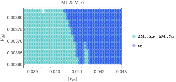
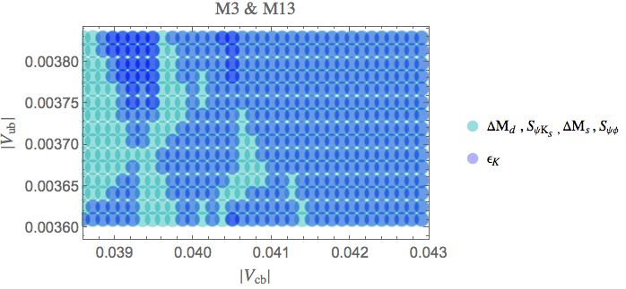
Figure 1: Allowed $(|V_{cb}|,|V_{ub}|)$ ranges in the parameter space of M1 and M16 (upper plot) and in that of M3 and M13 (lower plot). Each point corresponds to a set of 331 parameters. The green points are obtained after imposing the constraints on $\Delta M_{d},\,S_{\psi K_{s}},\,\Delta M_{s},\,S_{\psi\phi}$, while the light blue points derive from imposing the constraint on $\varepsilon_{K}$.

4.2 $C_{9}^{\text{NP}}$ and $C_{10}^{\text{NP}}$

We have already remarked the nice feature of 331 models that the ratio $C_{9}^{\text{NP}}/C_{10}^{\text{NP}}$ depends only on the considered scenario but not on the parameters $\tilde{s}_{13},\,\delta_{1},\,\tilde{s}_{23},\,\delta_{2}$. However, the separate values of $C_{9}^{\text{NP}}$ and $C_{10}^{\text{NP}}$ depend on them. In Fig. 2 we show the correlation between their real parts in the four scenarios, while in Fig. 3 the correlation between their imaginary parts is displayed.

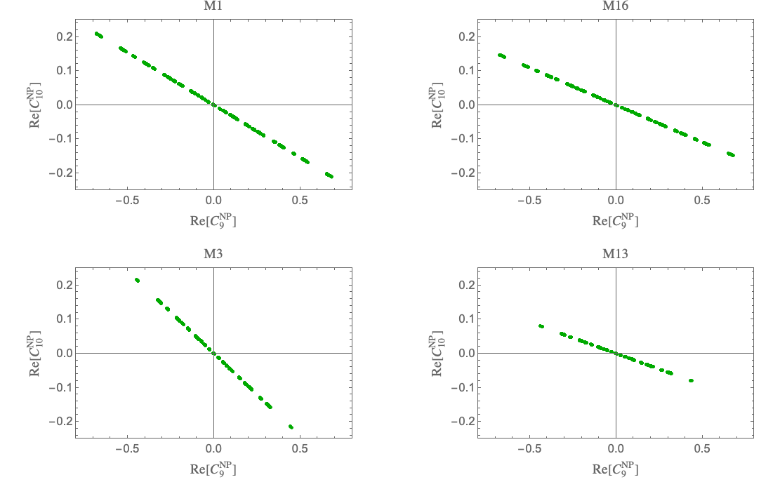
Figure 2: Correlation between the real parts of $C_{9}^{NP}$ and $C_{10}^{NP}$ in the four considered 331 models.

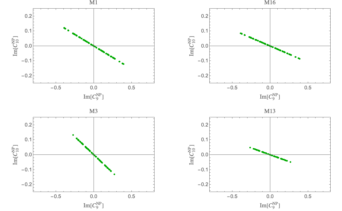
Figure 3: Correlation between the imaginary parts of $C_{9}^{NP}$ and $C_{10}^{NP}$ in the four considered 331 models.

In order to understand which values of $|V_{cb}|$ correspond to the largest deviations in $C_{9}^{\text{NP}}$ we consider ${\rm Max}\left|{\rm Re}[C_{9}^{\text{NP}}]\right|$ setting $|V_{ub}|$ at its central value. The result is shown in Fig. 4.

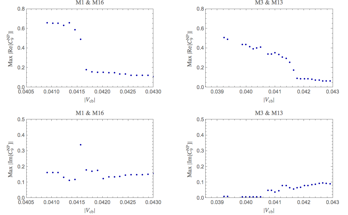
Figure 4: Maximal deviation of $\left|{\rm Re}[C_{9}^{NP}]\right|$ and $\left|{\rm Im}[C_{9}^{NP}]\right|$ in the four considered 331 models.

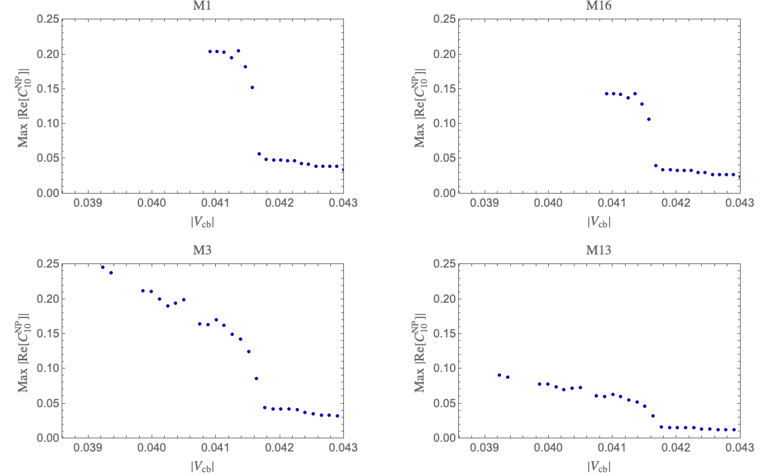
Figure 5: Maximal deviation of $\left|{\rm Re}[C_{10}^{NP}]\right|$ in the four considered 331 models.

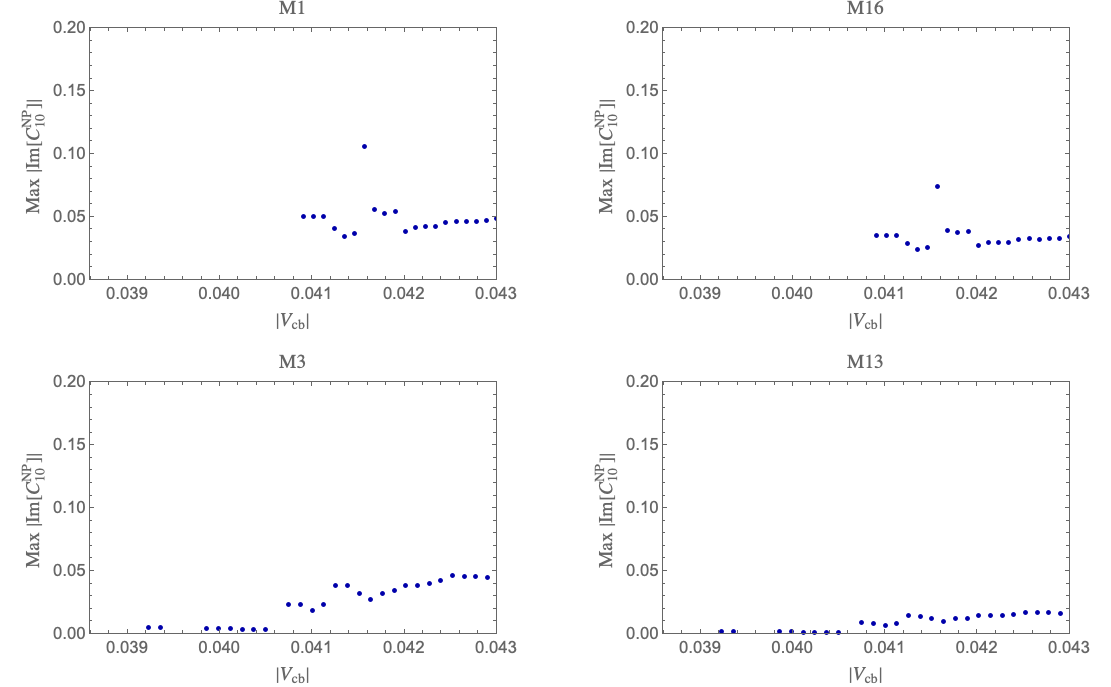
Figure 6: Maximal deviation of $\left|{\rm Im}[C_{10}^{NP}]\right|$ in the four considered 331 models.

These plots display that, consistently with the result in Fig. 1 in the case of M1 and M16 only the values $|V_{cb}|\geq 0.0405$ are allowed. Moreover, the deviation in $|{\rm Re}[C_{9}]|$ is a decreasing function of $|V_{cb}|$, as shown in Fig. 4, together with the plots for the imaginary part. This dependence on $|V_{cb}|$ follows from the fact, as seen in (4), that the experimental value of $\Delta M_{s}$ is best reproduced within the SM for $|V_{cb}|\approx 0.0426$ so that the room left for $Z^{\prime}$ contributions to $\Delta M_{s}$ decreases with increasing $|V_{cb}|$ and in turn not allowing sizeable impact on $C_{9}$.

The situation for $|{\rm Re}[C_{10}^{NP}]|$ and $|{\rm Im}[C_{10}^{NP}]|$ is displayed in Figs. 5 and 6. It can be noticed that $C_{9}^{NP}$ is to an excellent approximation the same in M1 and M16 on the one hand and in M3 and M13 on the other; for this reason we have shown the corresponding plots in a single figure. $C_{10}^{NP}$ is instead different in all the four considered cases.

We observe that while the pattern of NP contributions signalled by the data is correctly described by these models, the absolute values of $C_{9}^{\text{NP}}$ are likely to turn out to be too small to explain the observed suppression of the branching ratios for $B^{+}\to K^{+}\mu^{+}\mu^{-}$ and $B_{s}\to\phi\mu^{+}\mu^{-}$, in particular if the final value for $|V_{cb}|$ from tree-level decays will turn out to be in the ballpark of its inclusive determinations.

4.3 ${\bar{\cal B}}(B_{s}\to\mu^{+}\mu^{-})$ and ${\cal B}(B_{d}\to\mu^{+}\mu^{-})$

In Fig. 7 we plot the correlation between the rare decays ${\bar{\cal B}}(B_{s}\to\mu^{+}\mu^{-})$ and ${\cal B}(B_{d}\to\mu^{+}\mu^{-})$ in the four considered 331 models. In these plots, the gray region is obtained considering all the allowed parameter space in each scenario, while the red region corresponds to $|V_{cb}|\in[0.0386,\,0.0398]$ and the cyan region to $|V_{cb}|\in[0.0422,\,0.043]$. The SM results for $|V_{cb}|=0.03921$ and $|V_{cb}|=0.0426$ are also displayed. Comparing the four models, we can observe that if $|V_{cb}|$ is fixed consistently with the exclusive determinations, a possible suppression of both branching ratios with respect to their SM values, that is not yet excluded in view of large experimental errors, could be explained only in M3 and M13. On the other hand, inclusive values of $|V_{cb}|$ do not define a clear situation in any of the four models: other correlations should be explored in order to discriminate among these scenarios. We detail the dependence of the considered branching fractions on the CKM elements in the contour plots in Fig. 8 for M1 and M16 and in Fig. 9 for M3 and M13. Since in each scenario the parameter space involves 6 variables it is possible that fixing $(|V_{cb}|,\,|V_{ub}|)$ different values for the considered branching ratios are obtained, because these depend also on the other four parameters of the 331 model. Therefore, what is plotted in Fig. 8 and in Fig. 9 is the value of the branching ratios that, for a given pair $(|V_{cb}|,\,|V_{ub}|)$, mostly deviates from the corresponding SM prediction. The resulting value of the branching fractions can be read from the legends on the right of each plot. The benefit of these plots with respect to those already shown is that it is possible to relate a given value of the branching fractions to the entries for $(|V_{cb}|,\,|V_{ub}|)$, an information that is hidden in Fig. 7. The SM result as function of $(|V_{cb}|,\,|V_{ub}|)$ can be read from Fig. 10: comparison between these plots and the corresponding one in a given 331 model would give an idea of the possible deviation as a function of $(|V_{cb}|,\,|V_{ub}|)$. In particular, one can observe that M3 and M13 perform rather similarly to the SM, with values of the branching fractions that increase with $|V_{cb}|$ almost independently on $|V_{ub}|$. On the other hand, this pattern is not followed in M1 and M16.

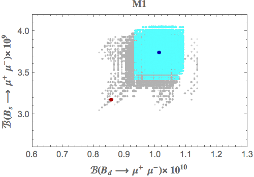
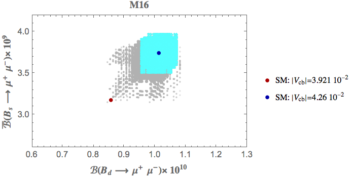
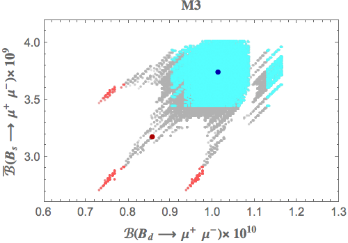
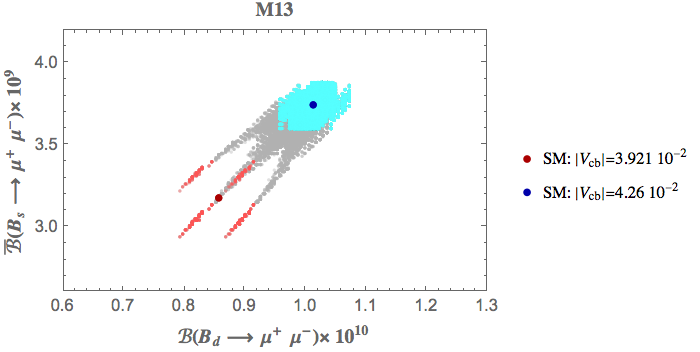
Figure 7: Correlation between ${\bar{\cal B}}(B_{s}\to\mu^{+}\mu^{-})$ and ${\cal B}(B_{d}\to\mu^{+}\mu^{-})$. The gray points span all the allowed parameter space in each scenario. The red region corresponds to $|V_{cb}|\in[0.0386,\,0.0398]$ while the cyan region corresponds to $|V_{cb}|\in[0.0422,\,0.043]$. The SM results in correspondence of two values of $|V_{cb}|$ are displayed, as specified in the legends.

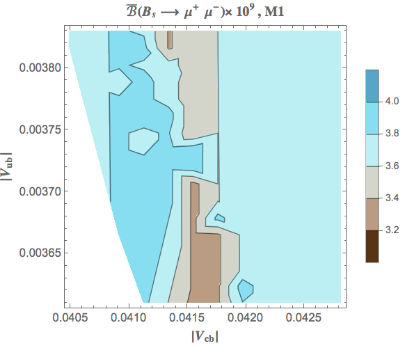
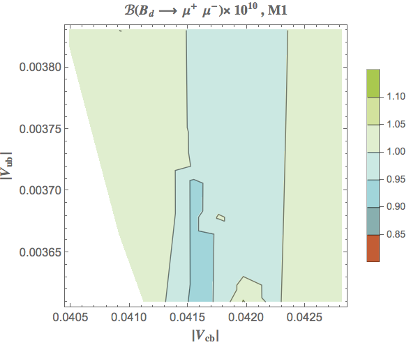
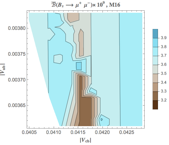
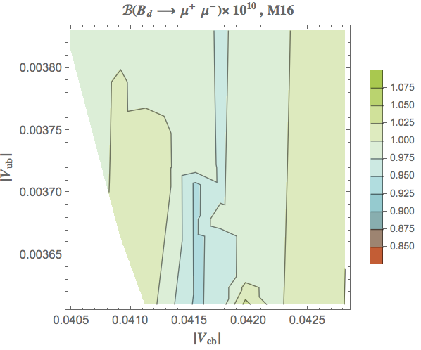
Figure 8: Contour Plots of ${\bar{\cal B}}(B_{s}\to\mu^{+}\mu^{-})$ (left column) and ${\cal B}(B_{d}\to\mu^{+}\mu^{-})$ (right column) versus $|V_{cb}|$ and $|V_{ub}|$ in M1 (upper plots) and in M16 (lower plots).

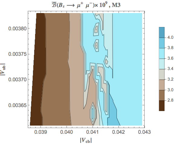
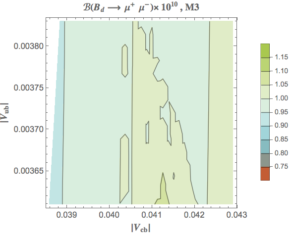
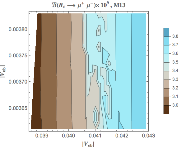
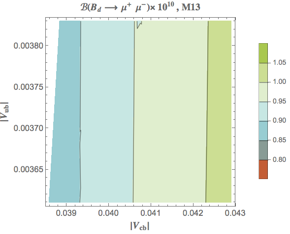
Figure 9: Contour Plots of ${\bar{\cal B}}(B_{s}\to\mu^{+}\mu^{-})$ (left column) and ${\cal B}(B_{d}\to\mu^{+}\mu^{-})$ (right column) versus $|V_{cb}|$ and $|V_{ub}|$ in M3 (upper plots)and in M13 (lower plots).

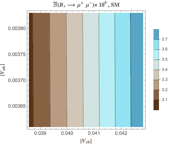
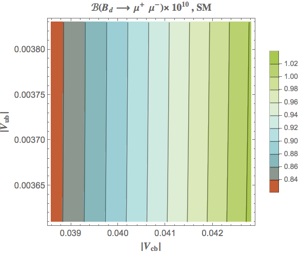
Figure 10: Contour Plots of ${\bar{\cal B}}(B_{s}\to\mu^{+}\mu^{-})$ (left column) and ${\cal B}(B_{d}\to\mu^{+}\mu^{-})$ (right column) versus $|V_{cb}|$ and $|V_{ub}|$ in the SM .

4.4 Rare Kaon decays

In Fig. 11 we display the correlation between ${\cal B}(K^{+}\to\pi^{+}\nu\bar{\nu})$ and ${\cal B}(K_{L}\to\pi^{0}\nu\bar{\nu})$. The gray points span all the allowed parameter space in each scenario, while the red region corresponds to $|V_{cb}|\in[0.0386,\,0.0398]$ and the cyan region to $|V_{cb}|\in[0.0422,\,0.043]$. The SM results for $|V_{cb}|=3.921\,10^{-2}$ and $|V_{cb}|=4.26\,10^{-2}$ are also displayed. In all the four models, the largest deviation from SM is possible in the case of ${\cal B}(K_{L}\to\pi^{0}\nu\bar{\nu})$. Contour plots analogous to those presented for $B_{s},\,B_{d}$ decays are shown in Figs. 12 and 13, to be compared with the corresponding SM case in Fig. 14. We observe again that M3 and M13 behave similarly to the SM, while M1 and M16 show a different pattern.

Correlation between ${\cal B}(K^{+}\to\pi^{+}\nu\bar{\nu})$ and ${\bar{\cal B}}(B_{s}\to\mu^{+}\mu^{-})$ is shown in Fig. 15. It can be observed that in all the four cases the inclusive values of $|V_{cb}|$ correspond to points that can be compatible with the experimental result for ${\bar{\cal B}}(B_{s}\to\mu^{+}\mu^{-})$ performing slightly better than the SM; such points correspond to ${\cal B}(K^{+}\to\pi^{+}\nu\bar{\nu})\leq 10^{10}$. Exclusive values of $|V_{cb}|$ that are not allowed in M1 and M16, can produce in M3 and M13 also values of ${\bar{\cal B}}(B_{s}\to\mu^{+}\mu^{-})$ and ${\cal B}(K^{+}\to\pi^{+}\nu\bar{\nu})$ simultaneously smaller than the experimental range.

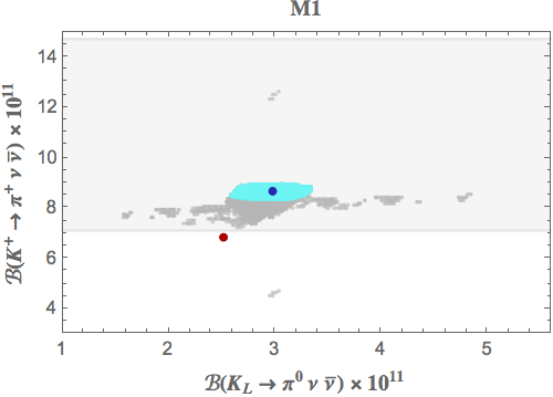
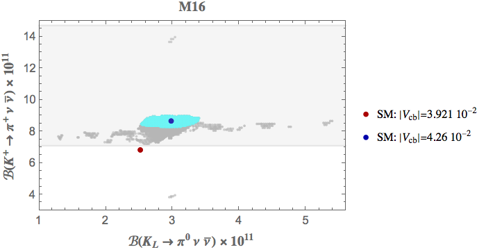
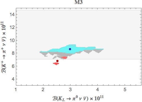
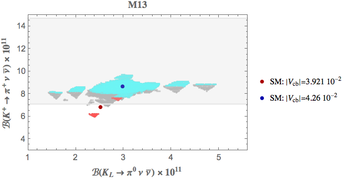
Figure 11: Correlation between ${\cal B}(K^{+}\to\pi^{+}\nu\bar{\nu})$ and ${\cal B}(K_{L}\to\pi^{0}\nu\bar{\nu})$. The gray points span all the allowed parameter space in each scenario. The red region corresponds to $|V_{cb}|\in[0.0386,\,0.0398]$ while the cyan region corresponds to $|V_{cb}|\in[0.0422,\,0.043]$. The SM results in correspondence of two values of $|V_{cb}|$ are displayed, as specified in the legends. The light gray region corresponds to the experimental range for ${\cal B}(K^{+}\to\pi^{+}\nu\bar{\nu})$ reported in Table 1.

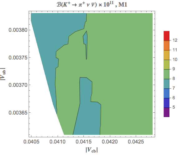
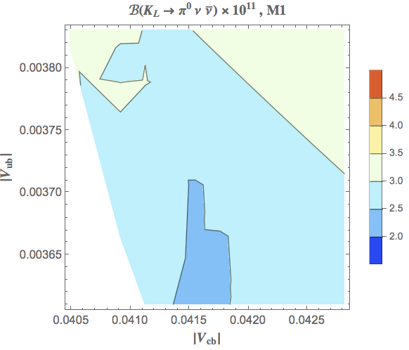
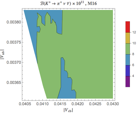
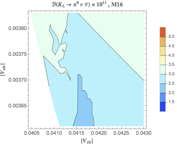
Figure 12: Contour Plots of ${\cal B}(K^{+}\to\pi^{+}\nu\bar{\nu})$ (left column) and ${\cal B}(K_{L}\to\pi^{0}\nu\bar{\nu})$ (right column) versus $|V_{cb}|$ and $|V_{ub}|$ in M1 (upper plots) and in M16 (lower plots).

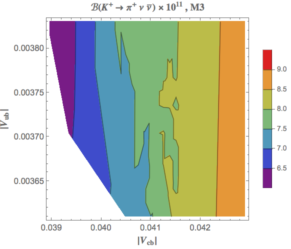
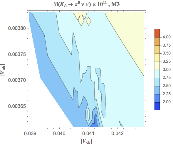
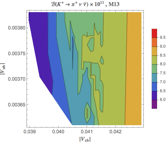
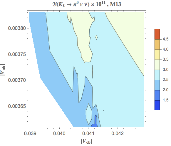
Figure 13: Contour Plots of ${\cal B}(K^{+}\to\pi^{+}\nu\bar{\nu})$ (left column) and ${\cal B}(K_{L}\to\pi^{0}\nu\bar{\nu})$ (right column) versus $|V_{cb}|$ and $|V_{ub}|$ in M3 (upper plots)and in M13 (lower plots).

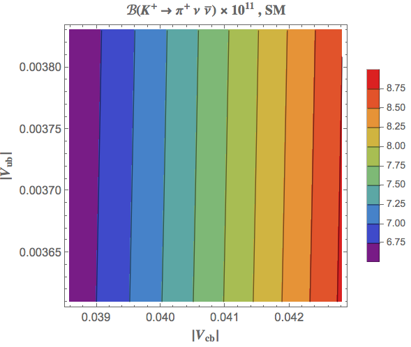
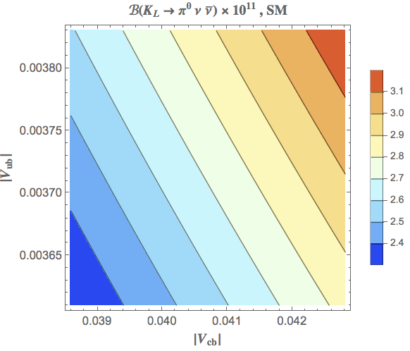
Figure 14: Contour Plots of ${\cal B}(K^{+}\to\pi^{+}\nu\bar{\nu})$ (left column) and ${\cal B}(K_{L}\to\pi^{0}\nu\bar{\nu})$ (right column) versus $|V_{cb}|$ and $|V_{ub}|$ in the SM .

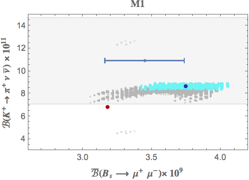
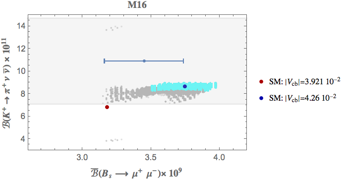
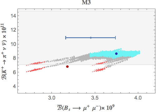
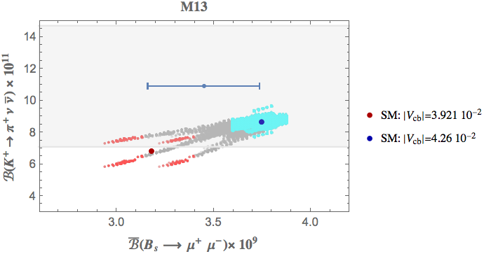
Figure 15: Correlation between ${\cal B}(K^{+}\to\pi^{+}\nu\bar{\nu})$ and ${\bar{\cal B}}(B_{s}\to\mu^{+}\mu^{-})$. The gray points span all the allowed parameter space in each scenario. The red region corresponds to $|V_{cb}|\in[0.0386,\,0.0398]$ while the cyan region corresponds to $|V_{cb}|\in[0.0422,\,0.043]$. The SM results in correspondence of two values of $|V_{cb}|$ are displayed, as specified in the legends. The light gray region and the blue range correspond to the experimental range for ${\cal B}(K^{+}\to\pi^{+}\nu\bar{\nu})$ and ${\bar{\cal B}}(B_{s}\to\mu^{+}\mu^{-})$, respectively, reported in Table 1.

5 Summary

Motivated by several changes both on experimental and theoretical frontiers we updated our 2016 analysis of various flavour observables in the 331 model based on the gauge group $SU(3)_{C}\times SU(3)_{L}\times U(1)_{X}$ for $M_{Z^{\prime}}=3\,{\rm TeV}$, that is still in the LHC reach.

Among 24 331 models considered in our 2016 analysis only four, namely M1, M3, M13 and M16 are simultaneously consistent with the electroweak precision tests and the relation between $C_{9}^{\text{NP}}$ and $C_{10}^{\text{NP}}$ signalled by the most recent data on the $B\to\mu^{+}\mu^{-}$ decay from the CMS.

The lessons from this analysis are as follows:

• The 331 models allow for the values of the ratio $C_{9}^{\text{NP}}/C_{10}^{\text{NP}}$ that are consistent with the most recent data. M13 and M16 are performing best but this can only be decided when new overall fits will be performed.

• However, only models M1 and M16 can reach the values ${\rm Re}[C_{9}^{\text{NP}}]=-0.7$, which although likely not quite sufficient to explain properly the the suppression of $b\to s\mu^{+}\mu^{-}$ branching ratios, they reproduce a significant portion of it. For M3 and M13 models only the corresponding values of $-0.5$ can be reached.

• Moreover, we notice that while in the case M1 and M16 models the maximal negative shifts of ${\rm Re}[C_{9}]$ can still be obtained for inclusive values in the ballpark of $|V_{cb}|=0.0415$, in the case of M3 and M13 the shift of $-0.5$ can only be obtained for exclusive values of $|V_{cb}|$ as low as $0.039$. We conclude then that models M1 and M16 perform best in this context but as seen in Fig. 4 for the case of the HYBRID scenario for CKM parameters none of the models can provide suppression of ${\rm Re}[C_{9}]$ by more than $-0.2$ which appears too small from present perspective.

• Concerning ${\rm Re}[C_{10}^{\text{NP}}]$ all models show only a small shift which is consistent with the data. This is also the case of of the imaginary parts of both $C_{9}^{\text{NP}}$ and $C_{10}^{\text{NP}}$.

• As seen in Fig 11, NP effects in $K^{+}\rightarrow\pi^{+}\nu\bar{\nu}$ turn out to be small but could be significantly larger in $K_{L}\rightarrow\pi^{0}\nu\bar{\nu}$.

We are looking forward to improved data on all observables to be able to judge better the ability of the 331 models in explaining signs of NP.

References

- [1] A. J. Buras, Gauge Theory of Weak Decays. Cambridge University Press, 6, 2020.
- [2] F. Pisano and V. Pleitez, An SU(3) x U(1) model for electroweak interactions, Phys. Rev. D46 (1992) 410–417, [hep-ph/9206242].
- [3] P. H. Frampton, Chiral dilepton model and the flavor question, Phys. Rev. Lett. 69 (1992) 2889–2891.
- [4] V. Pleitez, Challenges for the 3-3-1 models, in 5th Colombian Meeting on High Energy Physics, 12, 2021. arXiv:2112.10888.
- [5] A. E. Cárcamo Hernández, L. Duarte, A. S. de Jesus, S. Kovalenko, F. S. Queiroz, C. Siqueira, Y. M. Oviedo-Torres, and Y. Villamizar, When Flavor Changing Interactions Meet Hadron Colliders, arXiv:2208.08462.
- [6] A. J. Buras and E. Venturini, The exclusive vision of rare K and B decays and of the quark mixing in the standard model, Eur. Phys. J. C 82 (2022), no. 7 615, [arXiv:2203.11960].
- [7] R. J. Dowdall, C. T. H. Davies, R. R. Horgan, G. P. Lepage, C. J. Monahan, J. Shigemitsu, and M. Wingate, Neutral -meson mixing from full lattice QCD at the physical point, Phys. Rev. D 100 (2019), no. 9 094508, [arXiv:1907.01025].
- [8] A. J. Buras and F. De Fazio, 331 Models Facing the Tensions in Processes with the Impact on , and , JHEP 08 (2016) 115, [arXiv:1604.02344].
- [9] M. Blanke and A. J. Buras, Universal Unitarity Triangle 2016 and the tension between and in CMFV models, Eur. Phys. J. C76 (2016), no. 4 197, [arXiv:1602.04020].
- [10] N. Gubernari, M. Reboud, D. van Dyk, and J. Virto, Improved theory predictions and global analysis of exclusive processes, JHEP 09 (2022) 133, [arXiv:2206.03797].
- [11] LHCb Collaboration, Test of lepton universality in decays, arXiv:2212.09152.
- [12] LHCb Collaboration, Measurement of lepton universality parameters in and decays, arXiv:2212.09153.
- [13] LHCb Collaboration, R. Aaij et al., Simultaneous determination of CKM angle and charm mixing parameters, JHEP 12 (2021) 141, [arXiv:2110.02350].
- [14] A. J. Buras and E. Venturini, Searching for New Physics in Rare and Decays without and Uncertainties, Acta Phys. Polon. B 53 (9, 2021) A1, [arXiv:2109.11032].
- [15] A. J. Buras, Standard Model Predictions for Rare K and B Decays without New Physics Infection, arXiv:2209.03968.
- [16] M. Bordone, B. Capdevila, and P. Gambino, Three loop calculations and inclusive , Phys. Lett. B 822 (2021) 136679, [arXiv:2107.00604].
- [17] NA62 Collaboration, M. Zamkovský et al., Measurement of the very rare decay, PoS DISCRETE2020-2021 (2022) 070.
- [18] KOTO Collaboration, J. Ahn et al., Search for the and decays at the J-PARC KOTO experiment, Phys. Rev. Lett. 122 (2019), no. 2 021802, [arXiv:1810.09655].
- [19] LHCb Collaboration, R. Aaij et al., Improved limit on the branching fraction of the rare decay , Eur. Phys. J. C77 (2017), no. 10 678, [arXiv:1706.00758].
- [20] LHCb Collaboration, R. Aaij et al., Measurement of the decay properties and search for the and decays, arXiv:2108.09283.
- [21] CMS Collaboration, Combination of the ATLAS, CMS and LHCb results on the decays, CMS-PAS-BPH-20-003.
- [22] ATLAS Collaboration, Combination of the ATLAS, CMS and LHCb results on the decays., ATLAS-CONF-2020-049.
- [23] HFLAV Collaboration, Y. Amhis et al., Averages of -hadron, -hadron, and -lepton properties as of 2021, arXiv:2206.07501.
- [24] Particle Data Group Collaboration, P. A. Zyla et al., Review of Particle Physics, PTEP 2020 (2020), no. 8 083C01.
- [25] A. J. Buras, F. De Fazio, and J. Girrbach-Noe, Z-Z’ mixing and Z-mediated FCNCs in Models, JHEP 1408 (2014) 039, [arXiv:1405.3850].
- [26] A. J. Buras, F. De Fazio, J. Girrbach, and M. V. Carlucci, The Anatomy of Quark Flavour Observables in 331 Models in the Flavour Precision Era, JHEP 1302 (2013) 023, [arXiv:1211.1237].
- [27] A. J. Buras, F. De Fazio, and J. Girrbach, 331 models facing new data, JHEP 1402 (2014) 112, [arXiv:1311.6729].
- [28] A. J. Buras and F. De Fazio, in 331 Models, JHEP 03 (2016) 010, [arXiv:1512.02869].
- [29] P. Colangelo, F. De Fazio, and F. Loparco, transitions of Bc mesons: 331 model facing Standard Model null tests, Phys. Rev. D 104 (2021), no. 11 115024, [arXiv:2107.07291].
- [30] A. J. Buras, P. Colangelo, F. De Fazio, and F. Loparco, The charm of 331, JHEP 10 (2021) 021, [arXiv:2107.10866].
- [31] Flavour Lattice Averaging Group Collaboration, S. Aoki et al., FLAG Review 2019: Flavour Lattice Averaging Group (FLAG), Eur. Phys. J. C 80 (2020), no. 2 113, [arXiv:1902.08191].
- [32] Y. Aoki et al., FLAG Review 2021, arXiv:2111.09849.
- [33] J. Brod, M. Gorbahn, and E. Stamou, Updated Standard Model Prediction for and , in 19th International Conference on B-Physics at Frontier Machines, 5, 2021. arXiv:2105.02868.
- [34] J. Brod, M. Gorbahn, and E. Stamou, Standard-Model Prediction of with Manifest Quark-Mixing Unitarity, Phys. Rev. Lett. 125 (2020), no. 17 171803, [arXiv:1911.06822].
- [35] A. J. Buras, D. Guadagnoli, and G. Isidori, On beyond lowest order in the Operator Product Expansion, Phys. Lett. B688 (2010) 309–313, [arXiv:1002.3612].
- [36] A. J. Buras, M. Jamin, and P. H. Weisz, Leading and next-to-leading QCD corrections to parameter and mixing in the presence of a heavy top quark, Nucl. Phys. B347 (1990) 491–536.
- [37] J. Urban, F. Krauss, U. Jentschura, and G. Soff, Next-to-leading order QCD corrections for the mixing with an extended Higgs sector, Nucl. Phys. B523 (1998) 40–58, [hep-ph/9710245].
- [38] Heavy Flavor Averaging Group (HFAG) Collaboration, Y. Amhis et al., Averages of -hadron, -hadron, and -lepton properties as of summer 2016, arXiv:1612.07233.